Immediate recapture in the trapping-detrapping process of a single charge carrier

Abstract

Previously we have shown that pure 1/f noise arises from the trapping-detrapping process when traps are heterogeneous. Namely, the trapping-detrapping process relies on the assumption that detrapping rates of individual trapping centers in the condensed matter are random and uniformly distributed. Another assumption underlying the trapping-detrapping process was that both trapping and detrapping times need to have non–zero duration. Here we violate the latter assumption by introducing immediate recapture of the charge carrier. We show that 1/f noise will still be observed, though the range of frequencies over which it will be observed shifts to the lower frequency range as the immediate recapture probability increases.

1 Introduction

The white noise and the Brownian noise are two most well understood examples of noise and fluctuations in the various materials and devices [1]. White noise most typically arises from thermal fluctuations, or the discrete nature of detected particles (i.e., shot noise). It is characterized by an absence of temporal correlations, and a flat power spectral density (abbr. PSD). The Brownian noise is a temporal integral of the white noise, and consequently exhibits no correlations between the increments of the signal. The Brownian noise is short–term correlated, and exhibits PSD of the $S\left(f\right)\sim 1/f^{2}$ form. Yet in various materials and devices, especially in the low frequency range, PSD of $S\left(f\right)\sim 1/f^{\beta}$ (with $0.5<\beta<1.5$) form is often observed. The nature of this noise, in the literature often referred to as $1/f$ noise, flicker noise, or pink noise, remains an open question [2, 3, 4, 5, 6, 7, 8].

Here we extend a model of $1/f$ noise based on the trapping–detrapping process in the condensed matter [9, 10]. Unlike in numerous previous works (e.g., [11, 12, 13, 14]) $1/f$ noise in this particular process arises not from the superposition of independent relaxation processes, but from a drift of a single charge carrier. The quick overview of this model is given in Section 2. In Section 3 we introduce immediate recapture mechanism, which violates a core assumption underlying the original trapping–detrapping process. The recapture mechanism allows to have zero trapping times, and thus effectively implements “touching” gaps. In Section 4 we examine similar mechanism, which allows to have zero detrapping times, and thus effectively implements “touching” pulses. Analytically we show that these mechanisms do not prevent observation of $1/f$ noise, they just change the range of frequencies over which pure $1/f$ noise is observed. Outside this range PSD either saturates (for lowest frequencies) or decays as the Brownian noise. We supplement our analytical derivations by conducting numerical simulations. The results are summarized and conclusions are provided in Section 5.

2 Trapping–detrapping process

In contrast to the numerous previous works [11, 12, 13, 14], which consider superposition of independent relaxation processes, let us consider trapping–detrapping process of a single charge carrier (e.g., electron) drifting through the condensed matter. In what follows we assume that the charge carrier can either drift through the conduction band (thus generating electric current), or be trapped within a trapping center (thus no current is observed). Under these assumptions, the electric current (the observed signal) generated by the charge carrier will be a sequence of non–overlapping rectangular pulses. A sample of such signal is shown in Fig. 1.

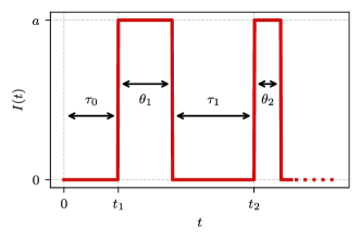
Figure 1: Sample signal generated by the trapping–detrapping of a single charge carrier. Relevant notation: $\tau_{i}$ – detrapping time (gap duration), $\theta_{i}$ – trapping time (pulse duration), $a$ – current generated by a free–drifting charge carrier (pulse height).

In Fig. 1, and further, $\tau_{i}$ stands for $i$-th detrapping time, $\theta_{i}$ stands for $i$-th trapping time (when written without the indices $\tau$ and $\theta$ will stand for the detrapping and trapping times in general). Note that, detrapping and trapping times are random variates sampled from the preselected distributions. On the other hand, we assumed that value of $a$ is predetermined and fixed through the simulation.

The process will generate current $I\left(t\right)$ composed of non–overlapping rectangular pulses with profiles $A_{k}\left(t\right)$. PSD of such signal is given by

$$S\left(f\right)=\lim_{T\rightarrow\infty}\left\langle\frac{2}{T}\left|\int_{0}^{T}I\left(t\right)e^{-2\pi\mathrm{i}ft}\operatorname{d}t\right|^{2}\right\rangle=\lim_{T\rightarrow\infty}\left\langle\frac{2}{T}\left|\sum_{k}e^{-2\pi\mathrm{i}ft_{k}}\mathcal{F}\left\{A_{k}\left(t-t_{k}\right)\right\}\right|^{2}\right\rangle.$$ (1)

In the above $T$ stands for the observation time, $t_{k}$ stands for time when $k$-the pulse starts, while $\mathcal{F}\left\{A_{k}\left(t-t_{k}\right)\right\}$ is the Fourier transform of the $k$-th pulse profile. Given the details of the process considered here the pulses will differ only by their duration. As the individual trapping and detrapping times are assumed to be independent, the PSD of $I\left(t\right)$ is determined purely by pulse height and the trapping and detrapping time distributions (let $\chi_{\theta}\left(\theta\right)$ and $\chi_{\tau}\left(\tau\right)$ be the respective characteristic functions). Under these considerations the PSD is given by [9]

$$S\left(f\right)=\frac{a^{2}\bar{\nu}}{\pi^{2}f^{2}}\operatorname{Re}\left[\frac{\left(1-\chi_{\theta}\left(f\right)\right)\left(1-\chi_{\tau}\left(f\right)\right)}{1-\chi_{\theta}\left(f\right)\chi_{\tau}\left(f\right)}\right],$$ (2)

with $\bar{\nu}$ being the mean number of pulses per unit time.

Typically when trapping–detrapping processes are considered [15] it is assumed that both $\tau_{i}$ and $\theta_{i}$ are sampled from the same distribution. Most often an exponential distribution is used with rates $\gamma_{\tau}$ and $\gamma_{\theta}$ respectively. This model would produce a Lorentzian PSD [15].

Instead let us assume that the detrapping rates $\gamma_{\tau}$ are uniformly distributed in $\left[\gamma_{\text{min}},\gamma_{\text{max}}\right]$. Implying that individual capture centers are heterogeneous, and are characterized by their own individual detrapping rate. In this case the distribution of the detrapping times is a continuous mixture of exponential distributions with different values of the rate parameter (see Fig. 2). Then the probability density function (abbr. PDF) of detrapping time $\tau$ is given by:

$$p\left(\tau\right)=\frac{1}{\gamma_{\text{max}}-\gamma_{\text{min}}}\int_{\gamma_{\text{min}}}^{\gamma_{\text{max}}}\gamma_{\tau}\exp\left(-\gamma_{\tau}\tau\right)\operatorname{d}\gamma_{\tau}=\frac{\left(1+\gamma_{\text{min}}\tau\right)\exp\left(-\gamma_{\text{min}}\tau\right)-\left(1+\gamma_{\text{max}}\tau\right)\exp\left(-\gamma_{\text{max}}\tau\right)}{\left(\gamma_{\text{max}}-\gamma_{\text{min}}\right)\tau^{2}}.$$ (3)

For very short $\tau$ the PDF saturates, as does the exponential distribution for very short times. For extremely long $\tau$ the PDF also decays as an exponential function. For the intermediate values, $\frac{1}{\gamma_{\text{max}}}\ll\tau\ll\frac{1}{\gamma_{\text{min}}}$, power–law asymptotic $\tau^{-2}$ behavior is observed. Having $p\left(\tau\right)\sim\tau^{-2}$ is known to be one of the ingredients needed to obtain $1/f$ noise [16, 17, 18, 9]. In our particular case, it can be shown that for $\gamma_{\text{min}}\ll 2\pi f\ll\gamma_{\text{max}}$ pure $1/f$ noise is observed [10]

$$S\left(f\right)\approx\frac{a^{2}\bar{\nu}}{\gamma_{\text{max}}f}.$$ (4)

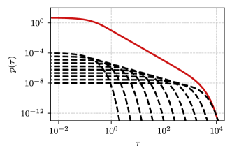
Figure 2: Probability density function of the detrapping time distribution under the assumption that individual detrapping rates are uniformly distributed in $\left[\gamma_{\text{min}},\gamma_{\text{max}}\right]$ (red curve), Eq. (3). The probability density function was obtained with $\gamma_{\text{min}}=10^{-3}$ and $\gamma_{\text{max}}=10$. Black dashed curves correspond to the exponential probability density functions with fixed rates: $\gamma_{\tau}=10^{-3}$, $2.78\times 10^{-3}$, $7.74\times 10^{-3}$, $2.15\times 10^{-2}$, $5.99\times 10^{-2}$, $1.67\times 10^{-1}$, $4.64\times 10^{-1}$, $1.29$, $3.59$, and $10$. Normalization of the exponential probability density functions was adjusted for the visualization purposes, but it remains proportional to their respective contributions.

3 Immediate recapture mechanism

Now let us assume that immediately after the charge carrier escapes, it may become immediately trapped with finite probability $r$. This implies that the trap is escaped after certain random number of attempts. Let $k$ be the number of attempts. It is trivial to show that $k$ follows geometric distribution, whose probability mass function is given by

$$p_{\text{geom}}\left(k\right)=r^{k-1}\left(1-r\right).$$ (5)

As charge carrier has made $k$ attempts to escape the trap, it has spent $\tau_{i}=\sum_{j=1}^{k}s_{j}$ time being trapped. Here $s_{j}$ would correspond to the detrapping time discussed in the previous section, but with a caveat that the next trapping time was zero. Instead of dealing with zero duration trapping times, let us simply consider that detrapping times are sampled from a different distribution, which takes into account the immediate recapture.

As immediate recapture is being made by the same trapping center, we assume that $s_{j}$ have same characteristic rate $\gamma_{\tau_{i}}$. Under these assumptions, $\tau_{i}$ for a fixed $k$ follows Erlang distribution. The characteristic function of Erlang distribution is given by

$$\chi_{\text{Erlang}}\left(f\right)=\left(\frac{\gamma_{\tau}}{\gamma_{\tau}-2\pi\mathrm{i}f}\right)^{k}.$$ (6)

Consequently the characteristic function of detrapping time distribution will be given by

$$\chi_{\tau}\left(f\right)=\sum_{k=1}^{\infty}\left[p_{\text{Geom}}\left(k;r\right)\chi_{\text{Erlang}}\left(f\right)\right]=\frac{\gamma_{\tau}\left(1-r\right)}{\gamma_{\tau}\left(1-r\right)-2\pi\mathrm{i}f}.$$ (7)

As can be seen from the above the immediate recapture mechanism simply rescales the rates by a factor of $1-r$. This observation allows us to reuse earlier results reported in [9, 10] simply by rescaling the rates, then:

$$S\left(f\right)\approx\frac{a^{2}\bar{\nu}}{\gamma_{\text{max}}\left(1-r\right)f}.$$ (8)

The approximation will hold as long as the characteristic trapping time is comparatively long $\gamma_{\theta}\ll\gamma_{\text{max}}\left(1-r\right)$, though the range of frequencies for which the approximation holds will shift towards the lower frequencies, and will apply to $\gamma_{\text{min}}\left(1-r\right)\ll 2\pi f\ll\text{$\gamma_{\text{max}}$$\left(1-r\right)$}$ range.

The analytical intuition above can be further supported by the numerical simulation shown in Fig. 3. In Fig. 3 power spectral densities obtained for different immediate recapture probabilities are shown rescaled in a manner that they would fall on the same curve, which corresponds to the original (no immediate recapture) case. Based on Eq. (7) we infer that the frequencies need to be divided by a factor of $1-r$, while the power spectral density itself needs to be multiplied by a factor of $\left(1-r\right)^{2}$ due to the mathematical form of Eq. (8):

$$\left(1-r\right)^{2}\times S\left(f\right)\approx\frac{a^{2}\bar{\nu}}{\gamma_{\text{max}}\frac{f}{\left(1-r\right)}}.$$ (9)

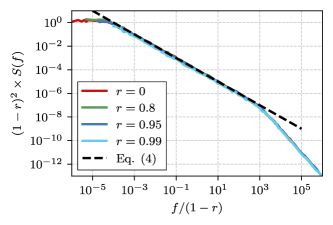
Figure 3: Rescaled simulated PSD curves of the trapping–detrapping process with immediate recapture mechanism. Common simulation parameters: $T=10^{6}$, $\gamma_{\text{min}}=10^{-4}$, $\gamma_{\text{max}}=10^{4}$, $a=1$, $\gamma_{\theta}=1$.

4 Immediate ejection mechanism

The general expression for the PSD of a signal with non–overlapping rectangular pulses, Eq. (2), is symmetric in respect to the trapping and detrapping time distributions. Namely, if $\chi_{\tau}\left(f\right)$ and $\chi_{\theta}\left(f\right)$ would be swapped in Eq. (2), then the expression remain the same. The assymetry is introduced into the model when different assumptions are being made about the distributions of the trapping and detrapping times. Though if we swap the assumptions (i.e., sample detrapping times from exponential distribution, and sample trapping times from Eq. (3)), the physical interpretation of the model would change, but the expression for the PSD would remain the same. In this section, instead of swapping the assumptions and studying the implications of immediate recapture mechanism again, let us consider it as an immediate ejection mechanism within the framework of the original model [9, 10].

Thus the model with immediate ejection, would have $\tau$ being sampled from a distribution whose PDF is given by Eq. (3), and $\theta$ being sampled from an exponential distribution with rate $\gamma_{\theta}$. Implementation of immediate ejection mechanism would mirror immediate recapture: as the charge carrier is captured by the capture center, it could be immediately released (ejected) with probability $r^{\prime}$. Following the same logic as for the immediate recapture mechanism, we obtain:

$$\chi_{\theta}\left(f\right) =\frac{\gamma_{\theta}\left(1-r^{\prime}\right)}{\gamma_{\theta}\left(1-r^{\prime}\right)-2\pi\mathrm{i}f}.$$ (10)

The approximation of PSD for the original model, Eq. (4), does not explicitly depend on $\gamma_{\theta}$. It is hidden behind the mean number of pulses per unit time:

$$\bar{\nu}=\frac{1}{\left\langle\theta\right\rangle+\left\langle\tau\right\rangle}.$$ (11)

If the trapping times are long in comparison to the detrapping times, i.e., $\left\langle\theta\right\rangle\gg\left\langle\tau\right\rangle$, then $\bar{\nu}\approx\left(1-r^{\prime}\right)\gamma_{\theta}$, while for the original model we would have $\bar{\nu}\approx\gamma_{\theta}$. The long trapping times assumption is not as restrictive as it may seem, because it is already known that pure $1/f$ noise can be observed only with long trapping times [9, 10]. Therefore for the model with immediate ejection, Eq. (4) should hold assuming that $\bar{\nu}$ is calculated appropriately.

In order to make the PSD curves corresponding to the cases with the different immediate ejection probabilities to fall on the same curve we need to scale the obtained PSDs by dividing every PSD curve by a factor of $1-r^{\prime}$. As expected, the simulated PSD curves fall on the same black dashed curve, which corresponds to Eq. (4). Though the numerical simulations contradict analytical intuition by showing that the range of frequencies over which Eq. (4) applies shrinks.

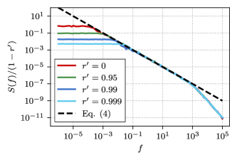
Figure 4: Rescaled simulated PSD curves of the trapping–detrapping process with immediate ejection mechanism. Common simulation parameters: $T=10^{6}$, $\gamma_{\text{min}}=10^{-4}$, $\gamma_{\text{max}}=10^{4}$, $a=1$, $\gamma_{\theta}=1$.

The shrinkage is caused by the fixed duration of the experiments. To verify this intuition, let us run numerical simulations, which are required to contain at least $N_{\text{min}}$ number of pulses, and have longer duration than $T_{\text{min}}$. Namely, the simulation is continued until both minimums are exceeded. Our simulations are similar to the conditional PSD measurements carried out in [19], but instead of scrapping the experiments we let them continue until both minimum conditions are met. As shown in Fig. 5 the overall shape of PSD is the same in all cases, only the intensity differs, as no rescaling is applied in this figure.

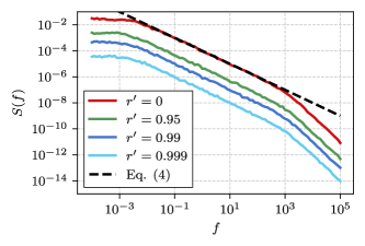
Figure 5: Simulated conditional PSD curves of the trapping–detrapping process with immediate ejection mechanism. Common simulation parameters: $T_{\text{min}}=10^{6}$, $N_{\text{min}}=10^{6}$, $\gamma_{\text{min}}=10^{-2}$, $\gamma_{\text{max}}=10^{4}$, $a=1$, $\gamma_{\theta}=1$.

5 Conclusions

We have examined the influence of the immediate recapture mechanism, and its mirror mechanism – the immediate ejection, on the spectral properties of the trapping–detrapping process exhibiting $1/f$ noise. We have shown that making the pulses, or the gaps, disappear doesn’t cause $1/f$ noise to become perverted as taking the point process limit of the process does [9, 10]. After appropriate rescaling of the signal intensity and the time scale, both mechanisms still produce PSDs well approximated by Eq. (4).

However, for the particular case of the immediate ejection mechanism, we have observed spurious shrinkage of the range of frequencies over which $1/f$ noise is observed. We have shown that the shrinkage is caused by the decreasing number of pulses being observed over the finite–duration experiments. This effect disappears if the conditional PSDs are measured. The simulated experiment is then required to have a certain minimum duration and to record a certain minimum number of pulses.

The ideas presented here can be taken further by allowing the individual pulses to not only “touch”, but also overlap. However, this will require new physical and mathematical formulation of the trapping–detrapping process. In particular, $\tau$ would have to be allowed to become negative, or its meaning would have to be redefined. Another possible future research direction would be examining the pulses with arbitrary profiles.

Author contributions

AK: Conceptualization, Methodology, Software, Writing, Visualization. BK: Conceptualization, Supervision.

References

- [1] S. Kogan, Electronic noise and fluctuations in solids, Cambridge University Press, 1996. doi:10.1017/CBO9780511551666.
- [2] R. F. Voss, J. Clarke, 1/f noise from systems in thermal qquilibrium, Physical Review Letters 36 (1) (1976) 42–45. doi:10.1103/PhysRevLett.36.42.
- [3] P. Dutta, P. M. Horn, Low-frequency fluctuations in solids: 1/f noise, Rev. Mod. Phys. 53 (1981) 497–516. doi:10.1103/RevModPhys.53.497.
- [4] M. Kobayashi, T. Musha, 1/f fluctuation of heartbeat period, IEEE Transactions on Biomedical Engineering 29 (1982) 456–457. doi:10.1109/TBME.1982.324972.
- [5] W. Li, D. Holste, Universal 1/f noise, crossovers of scaling exponents, and chromosome-specific patterns of guanine-cytosine content in DNA sequences of the human genome, Physical Review E 71 (4) (2005) 041910. doi:10.1103/PhysRevE.71.041910.
- [6] D. J. Levitin, P. Chordia, V. Menon, Musical rhythm spectra from Bach to Joplin obey a 1/f power law, Proceedings of the National Academy of Sciences of the United States of America 109 (2012) 3716–3720. doi:10.1073/pnas.1113828109.
- [7] Z. R. Fox, E. Barkai, D. Krapf, Aging power spectrum of membrane protein transport and other subordinated random walks, Nature Communications 12 (2021). doi:10.1038/s41467-021-26465-8.
- [8] G. Wirth, M. B. da Silva, T. H. Both, Unified compact modeling of charge trapping in 1/f noise, RTN and BTI, in: 2021 5th IEEE Electron Devices Technology and Manufacturing Conference (EDTM), IEEE, 2021, pp. 1–3. doi:10.1109/edtm50988.2021.9421005.
- [9] A. Kononovicius, B. Kaulakys, 1/f noise from the sequence of nonoverlapping rectangular pulses, Physical Review E 107 (2023) 034117. doi:10.1103/PhysRevE.107.034117.
- [10] A. Kononovicius, B. Kaulakys, noise from the trapping-detrapping process of individual charge carriers, available as arXiv:2306.07009 [math.PR] (2023). doi:10.48550/ARXIV.2306.07009.
- [11] J. Bernamont, Fluctuations in the resistance of thin films, Proceedings of the Physical Society 49 (4S) (1937) 138–139. doi:10.1088/0959-5309/49/4S/316.
- [12] A. van der Ziel, Flicker noise in electronic devices, in: Advances in Electronics and Electron Physics, Elsevier, 1979, pp. 225–297. doi:10.1016/s0065-2539(08)60768-4.
- [13] E. Milotti, 1/f noise: A pedagogical review, available as arXiv:physics/0204033 [physics.class-ph] (2002). arXiv:physics/0204033, doi:10.48550/arXiv.physics/0204033.
- [14] V. Palenskis, K. Maknys, Nature of low-frequency noise in homogeneous semiconductors, Scientific Reports 5 (1) (2015). doi:10.1038/srep18305.
- [15] V. Mitin, L. Reggiani, L. Varani, Generation-recombination noise in semiconductors, in: Noise and Fluctuation Controls in Electronic Devices, Noise and Fluctuation Controls in Electronic Devices, American Scientific Publishers, 2002.
- [16] G. Margolin, E. Barkai, Nonergodicity of a time series obeying Levy statistics, Journal of Statistical Physics 122 (1) (2006) 137–167. doi:10.1007/s10955-005-8076-9.
- [17] M. Lukovic, P. Grigolini, Power spectra for both interrupted and perennial aging processes, The Journal of Chemical Physics 129 (18) (2008) 184102. doi:10.1063/1.3006051.
- [18] M. Niemann, H. Kantz, E. Barkai, Fluctuations of 1/f noise and the low-frequency cutoff paradox, Physical Review Letters 110 (14) (2013) 140603. doi:10.1103/PhysRevLett.110.140603.
- [19] N. Leibovich, E. Barkai, Conditional noise: From single molecules to macroscopic measurement, Physical Review E 96 (3) (2017) 032132. doi:10.1103/PhysRevE.96.032132.