Nodal Volumes as Differentiable
Functionals of Gaussian fields

Abstract.

We characterize the absolute continuity of the law and the Malliavin-Sobolev regularity of random nodal volumes associated with smooth Gaussian fields on generic $\mathcal{C}^{2}$ manifolds with arbitrary dimension. Our results extend and generalize the seminal contribution by Angst and Poly (2020) about stationary fields on Euclidean spaces and cover, in particular, the case of two-dimensional manifolds, possibly with boundary and corners. The main tools exploited in the proofs include the use of Gaussian measures on Banach spaces, Morse theory, and the characterization of Malliavin-Sobolev spaces in terms of ray absolute continuity. Several examples are analyzed in detail.
Keywords: Gaussian meaures; Riemannian Geometry; Malliavin Calculus ; Nodal Volumes ; Random Fields ; Critical Points
AMS Classification: 60G15; 60H07; 60G60

1. Introduction

For the rest of the paper, and unless otherwise specified, every random element is assumed to be defined on an adequate common probability space $(\Omega,\mathfrak{S},\mathbb{P})$, with $\mathbb{E}$ indicating expectation with respect to $\mathbb{P}$.

1.1. Overview and motivation

The aim of this work is to develop new geometric and probabilistic tools for studying fine properties of random nodal volumes (that is, measures of vanishing loci) associated with smooth Gaussian random functions on compact Riemannian manifolds, with special emphasis on their differentiability and on the non-singularity of their laws. One of our main achievements (see Theorem 1.2, as well as Section 1.5, for a discussion) is an almost exhaustive characterization of random nodal volumes as elements of the Malliavin-Sobolev spaces $\mathbb{D}^{1,p}$ (see Section 3.2 below, as well as [21, Section 5.2] and [72, 75]), when $p\in\{1,2\}$. As demonstrated in the subsequent discussion, the approach developed in the present work naturally complements and extends the seminal contribution by J. Angst and G. Poly [7] — which provided the initial impetus for our research — where the absolute continuity of the laws of random nodal volumes was studied for the first (and unique!) time by using tools from the Malliavin calculus of variations.

The main findings of [7] can be summarized as follows. Let $m\geq 3$, and let $M$ be either the $m$-dimensional torus $(\mathbb{S}^{1})^{m}=\mathbb{T}^{m}$ or a closed rectangle in $\mathbb{R}^{m}$ of positive Lebesgue measure. We consider a centered Gaussian random field $f=\{f(x):x\in M\}$ such that $f$ is a.s. of class $\mathcal{C}^{2}$, stationary and unit variance. The nodal volume of $f$ is the random quantity $V(f):=\mathcal{H}^{m-1}(f^{-1}(0)\cap M)$, where $\mathcal{H}^{m-1}$ indicates the $(m-1)$–dimensional Haussdorff measure. The next statement, proved in [7], characterizes the smoothness of $V(f)$ in terms of Malliavin-Sobolev spaces (and yields the non-singularity of its law) under some natural further assumptions on $f$.

Theorem 1.1 (Theorems 1 and 2 in [7]).

In addition to the previous requirements, assume that the $m$-dimensional vector $\nabla f(0)$ has a density. Then: (i) $V(f)$ belongs to the Malliavin-Sobolev space $\mathbb{D}^{1,\eta}$ for all $\eta\in[1,\frac{m+1}{3})$, and (ii) its law has a non-zero component that is absolutely continuous with respect to the Lebesgue measure (and, therefore, $V(f)$ is not a.s. equal to a constant).

Note that the previous statement does not cover the case $m=2$. Classically, when coupled with stationarity, the requirement that $\nabla f(0)$ has a density implies that $0$ is a.s. a regular value of $f$, and therefore $f^{-1}(0)$ is a $(m-1)$-dimensional $\mathcal{C}^{2}$ (random) submanifold of $M$. The strategy adopted in [7] for proving the above statement hinges upon an elegant representation of $V(f)$ as a Riemann integral involving some smooth transformation of $f$ and its derivatives up to the order two (see [7, Proposition 7 and Section 4.5.1]). Such a closed formula can then be used to study the Malliavin-Sobolev regularity of $V(f)$ by leveraging the fact that each space $\mathbb{D}^{1,\eta}$ is the closure in an appropriate norm of the class of smooth cylindrical functions (see e.g. [75, Section 1.2] and [72, Section 2.3], as well as Section 3.2 below). Once the Malliavin smoothness of $V(f)$ is established, the non-singularity of its law follows by a classical criterion due to N. Bouleau (see [7, Theorem 4]).

The main idea developed in the sections to follow is that one can efficiently extend and generalize the results proved in [7] (in particular, covering the two-dimensional case) by directly exploiting the equivalent characterization of the space $\mathbb{D}^{1,p}$ ($p\geq 1$) as the collection of those random variables $\Psi=\Psi(f)\in L^{p}(\mathbb{P})$ verifying the three properties

1. $\Psi$ is ray absolutely continuous, meaning that, for every element $h$ of the Cameron-Martin space of $f$, the mapping $t\mapsto\Psi(f+th)$ admits an absolutely continuous modification;

2. $\Psi$ admits a Fréchet-type stochastic derivative, written $\mathrm{D}_{\mathscr{M}}\Psi$;

3. $\mathrm{D}_{\mathscr{M}}\Psi$ is integrable with respect to an appropriate norm (whose definition depends on the exponent $p$).

By construction, one has that $\mathbb{D}^{1,q}\subset\mathbb{D}^{1,p}$, for all $1\leq p<q$. The reader is referred to Definition 3.6 below, as well as [21, Definitions 5.2.3 and 5.2.4], for details; we observe that the fact that properties (a)–(c) fully characterize $\mathbb{D}^{1,p}$ is a deep result in infinite-dimensional Gaussian analysis (proved e.g. in [21, Thm. 5.7.2]), mirroring the usual characterization of classical Sobolev spaces in terms of “absolute continuity on lines”, see e.g. [50, Section 11.3]. Interestingly, our analysis will show that the study of the non-singularity of the law of $V(f)$ can be disentangled from the study of its Malliavin-Sobolev regularity, see Section 7.3 (in particular, Remark 7.8) for a full discussion of this point. To motivate the reader, we now present one of the general statements proved in our work — which represents a substantial extension of Theorem 1.1. For the rest of this section, we will use some notions and notation from differential geometry; see Section 4.2 below, and the references therein, for relevant definitions.

Theorem 1.2.

Let $M$ be a $\mathcal{C}^{2}$ compact Riemannian manifold with dimension $m\geq 2$ (possibly with boundary $\partial M$) and let $X=\{X(p):p\in M\}$ be a centered Gaussian field which is $\mathbb{P}$-a.s. of class $\mathcal{C}^{2}(M)$. Write $V(X):=\mathcal{H}^{m-1}(X^{-1}(0))$ for the nodal volume of $X$, and assume moreover that, for all $p\in M$ and all non-zero $v\in T_{p}M$, the Gaussian vector $(X(p),d_{p}X(v))\mathchoice{\raisebox{-1.50696pt}{$\displaystyle{{}^{\subset}}$}\mkern-11.5mu\raisebox{1.93747pt}{$\displaystyle{{}_{\subset}}$}}{\mkern 1.0mu\raisebox{-1.1625pt}{$\textstyle{{}^{\subset}}$}\mkern-11.7mu\raisebox{1.93747pt}{$\textstyle{{}_{\subset}}$}}{\raisebox{1.50696pt}{$\scriptstyle\subset$}\mkern-14.0mu\raisebox{-0.6458pt}{$\scriptstyle\subset$}}{\raisebox{1.29167pt}{$\scriptscriptstyle\subset$}\mkern-13.5mu\raisebox{-0.43057pt}{$\scriptscriptstyle\subset$}}\mathbb{R}^{2}$ admits a density. Then, $X^{-1}(0)$ is almost surely a neat $\mathcal{C}^{2}$ hypersurface and the following holds:

1. For all $m\geq 2$, $V(X)$ is square-integrable. Moreover, provided $V(X)$ is not $\mathbb{P}$-a.s. equal to a constant, one has that the law of $V(X)$ and the Lebesgue measure are not mutually singular, and the topological support of the law of $V(X)$ is a (possibly unbounded) interval. Finally, if the topological support of the law of $X$ is given by the whole set $\mathcal{C}^{2}(M)$, then there exist numbers $P\in(0,1)$, and a probability density $\pi(x)$ with support equal to $[0,+\infty)$ such that, for all Borel subset $I\subseteq\mathbb{R}$,

   (1.1) $$\mathbb{P}(V(X)\in I)=P\,\delta_{0}(I)+(1-P)\int_{I}\pi(x)\,dx,$$

   where $\delta_{0}$ is the Dirac mass in zero.

2. One has that $V(X)\in\mathbb{D}^{1,1}$ for $m\in\{2,3\}$, and $V(X)\in\mathbb{D}^{1,2}$ for all $m\geq 4$.

3. When $m=3$, a sufficient condition ensuring that $V(X)\in\mathbb{D}^{1,2}$ is that, for all $p\in M$ and all non-zero $v\in T_{p}M$, the Gaussian vector $(X(p),d_{p}X(v),{\rm Hess}_{p}X(v,v))$, with values in $\mathbb{R}^{3}$, admits a density.

4. When $m=2$, assume in addition that for every pair $p,q\in\partial M$, there exist $u\in T_{p}M,v\in T_{q}M$ such that the vectors $(X(p),d_{p}X(u))$ and $(X(q),d_{q}X(v))$ are not fully correlated; then, $V(X)\notin\mathbb{D}^{1,2}$, provided there exists no curve $Z\subset M$ such that $Z$ and $X^{-1}(0)$ are $\mathcal{C}^{1}$-isotopic in $M$ with probability 1.

Remark 1.3.

1. A hypersurface of a manifold with boundary is neat if it intersects the boundary in a transverse way, see Definition 4.4 from [40, Section 1.4]. The fact that $X^{-1}(0)$ is a neat $\mathcal{C}^{2}$ hypersurface is ensured by Proposition 4.5 and follows from Bulinskaya Lemma 5.2, by standard arguments.

2. Point (i) in Theorem 1.2 combines the contents of Theorem 7.6, Proposition 7.7, Corollary 9.1 and Theorem 10.1 below; Point (ii) follows from Theorems 9.2 and 9.5; Point (iii) is again a consequence of Theorem 9.2; finally, Point (iv) can be derived from Theorem 9.7. We observe that, in contrast to Theorem 1.1, our findings cover the case of two-dimensional manifolds, and do not involve any notion of stationarity.

3. As shown in Theorem 9.3, the content of Point (ii) (in the case $m\geq 3$) and Point (iii) extends to the case of a manifold $M$ with corners, therefore including the situation in which $M$ is a closed rectangle in $\mathbb{R}^{m}$. As a consequence, when applied to the case where $m\in\{3,4,5\}$ and $M$ is such a rectangle (or $M=\mathbb{T}^{m}$), the conclusions of Theorem 1.2 and of its extension to the cornered case, refine the content of Theorem 1.1-(i) (since, for $m\leq 5$, one has that $\frac{m+1}{3}\leq 2$).

4. The additional condition appearing at Point (iii), ensuring that $V(X)\in\mathbb{D}^{1,2}$ when $m=3$, is an artifact of our use of Kac-Rice formulae for checking the integrability of norms of stochastic derivatives — see the proof of Theorem 9.2 below. It seems plausible that such a restriction can eventually be lifted, and that the conclusion holds in full generality.

5. As already observed, since the Gaussian field $f$ considered in Theorem 1.1 is stationary and has positive variance, one can automatically conclude that the random variable $V(f)$ is not $\mathbb{P}$-a.s. constant. As discussed in [7, Section 3], such a result is a consequence of Bochner’s theorem which, in this case, allows one to directly characterize the topological support of $f$ in terms of the topological support of its spectral measure (see [7, Lemma 2]). At the level of generality of Theorem 1.2-(i), no equivalent of Bochner’s theorem is available and one has to explicitly assume that $V(X)$ is non-constant. We observe that the non-constancy of $V(X)$ is implied by the following property: the topological support of $X$ contains two functions $g_{1},g_{2}\in\mathcal{C}^{2}(M)$, such that $0$ is a regular value of $g_{1}$ and $g_{2}$, and $V(g_{1})\neq V(g_{2})$. Moreover, notice that if the zero set of a centered Gaussian field is almost surely empty, then it must be of the form $\gamma f$, for some $\gamma\sim\mathcal{N}(0,1)$ and $f\in\mathcal{C}^{2}(M)$. Under the hypotheses of Theorem 1.2, such situation is excluded, so that there exist always at least one function $g_{2}$ in the topological support of $X$ such that $V(g_{2})>0$. Consequently, if the topological support of $X$ contains some $g_{1}\in\mathcal{C}^{2}(M)$ such that $g_{1}^{-1}(0)=\emptyset$, then $V(X)$ is non-constant.

6. Consider the case $m=2$, and denote by $Y$ the random variable counting the number of connected components of the set $X^{-1}(0)$. Then, if $Y$ is not degenerate (that is, the distribution of $Y$ charges at least two integers with positive probability), one has that there is no curve $Z\subset M$ such that $X^{-1}(0)$ is isotopic to $Z$ (see [40, p. 178] or Definition 4.11) with probability one.

7. Note that relation (1.1) is equivalent to saying that, whenever $X$ has full support, $V(X)$ has the same law as $\epsilon\,W$, where $W$ is a random variable with density $\pi$ and $\epsilon$ is a Bernoulli random variable independent of $W$, with parameter $P$. Some partial characterization of the density $\pi$ — obtained by means of Malliavin calculus — is discussed in Section 1.4.1.

1.2. A short literature review

Local geometric quantities associated with nodal sets of Gaussian (and non-Gaussian) smooth random fields have been recently the object of an intense study — often in connection with outstanding open problems in differential geometry, like e.g. Yau’s conjecture (see e.g. [58, 88]) or Berry’s random wave conjecture (see e.g. [1, 16, 27, 33, 41]). The recent survey [87] contains a detailed overview of the literature, to which we refer the reader for further references and motivation.

The following list displays a sample of contributions that are directly relevant to the present work.

• As already mentioned, reference [7] contains the first study of the absolute continuity of the law of nodal volumes (for stationary fields on rectangles or on flat tori) by using Malliavin calculus. Some of the pivotal formulae in [7] have been subsequently extended by B. Jubin to a Riemannian setting in [42], where they are used to study the continuity of nodal volumes with respect to appropriate function space topologies.

• It is important to notice that the main findings of [7] and of the present work have a static nature, that is, they provide information about the distribution (and smoothness) of the nodal volume associated with some fixed random field. On the other hand, most existing results about the law of nodal volumes (and other local geometric quantities) have an asymptotic character, that is, they take the form of probabilistic limit theorems (such as laws of large numbers, as well as central and non-central limit theorems) obtained either by letting some “energy parameter” diverge to infinity, or by suitably expanding the domain of definition of the field. It is a remarkable fact that many central and non-central results deduced in this way make use of Wiener chaos expansions, which are in turn one of the fundamental building blocks of Malliavin-Sobolev spaces (see e.g. [75, Section 1.1] and [72, Section 2.7]). The reader is referred to the survey [79], as well as to [15, 44, 62, 63, 64, 73, 70, 77], for a collection of representative references – connected in particular to Berry’s seminal work [17] on cancellation phenomena; see [72] for a detailed analysis of the probabilistic techniques behind these results.

• In Section 9.1 and Section 8 we wil use Kac-Rice formulae in order to study, respectively, the square-integrability of random nodal volumes, and the integrability of stochastic derivatives with respect of appropriate Sobolev-type norms. While the content of Section 9.1 makes direct use of the recent findings from [34] (see also [56]), the results of Section 8 are technically more demanding, and require a careful study of the two-points Kac-Rice density associated to the stochastic derivative. As discussed at length in [87], Kac-Rice formulae have played a fundamental role in the proof of first- and second-order asymptotic results for nodal volumes of Gaussian random fields, and in particular for establishing tight upper and lower bounds on variances — see e.g. [17, 27, 45, 86] for some outstanding examples. The reader is referred to the monographs [2, 9, 18] (see also [84]) for a thorough introduction to this topic.

1.3. Standard assumptions

To simplify the discussion, we notice that most results concerning Gaussian fields contained in the present paper (see, in particular, Theorem 1.2) are stated under the following assumption.

Assumption A.

The set $M$ is a compact Riemannian manifold of dimension $m\geq 2$, possibly with boundary, and of class $\mathcal{C}^{2}$. Also, $X=\{X(p):p\in M\}$ is a centered Gaussian field defined on $M$, which is $\mathbb{P}$-a.s. of class $\mathcal{C}^{2}(M)$. Moreover, for all $p\in M$ and all non zero $v\in T_{p}M$, the two-dimensional Gaussian vector $(X(p),d_{p}X(v))$ admits a density.

In the context of Assumption A, the boundary of $M$ is denoted by $\partial M$, whereas the internal manifold is written ${\kern 0.0ptM}^{\mathrm{o}}$; in particular, $M=\partial M\sqcup{\kern 0.0ptM}^{\mathrm{o}}$.

1.4. First consequences and representative examples

1.4.1. Density formulae and growth estimates

Theorem 1.2 provides sufficient conditions ensuring that random nodal volumes belong to some space $\mathbb{D}^{1,\eta}$. The next statement, which is a consequence of Theorem 10.1, shows that, when $\eta=2$, one can infer an explicit form for the density $\pi(x)$ appearing in (1.1). In what follows, we write $\mathcal{H}_{X}$ to indicate the Cameron-Martin space associated with a Gaussian process $X$, and denote by ${\rm D}_{\mathscr{M}}F$ the Malliavin derivative of some $F\in\mathbb{D}^{1,\eta}$ (which is a random element with values in $\mathcal{H}_{X}^{*}\simeq\mathcal{H}_{X}$); see Section 3 for definitions. We also use the symbol $L^{-1}$ to indicate the pseudo-inverse of the generator of the Ornstein-Uhlenbeck semigroup, as defined e.g. in [72, Definition 2.8.10].

Theorem 1.4.

Let Assumption A prevail and assume in addition that the topological support of the law of $X$ is the full space $\mathcal{C}^{2}(M)$ and that $V(X)\in\mathbb{D}^{1,2}$. Then, writing $c=\mathbb{E}[V(X)]$ and $\bar{V}=V(X)-c$, one has that the density $\pi$ appearing in (1.1) has the form

(1.2) $$\pi(x+c)=\frac{\mathbb{E}|\bar{V}|}{2g(x)}\exp\left\{-\int_{0}^{x}\frac{y\,dy}{g(y)}\right\},$$

for $dx$-a.e. $x\in[-c,+\infty)$, where the function $g$ has the following properties:

1. $g(x)>0$, for $dx$-almost every $x\in(-c,\infty)$;

2. on the interval $(-c,\infty)$, $g$ is a version of the mapping

   (1.3) $$x\mapsto\mathbb{E}\big{[}\langle{\rm D}_{\mathscr{M}}V,-{\rm D}_{\mathscr{M}}L^{-1}V\rangle_{\mathcal{H}_{X}}\,|\,\bar{V}=x\big{]},$$

   and is uniquely defined up to sets of Lebesgue measure zero.

3. $\mathbb{E}[g(\bar{V})]<\infty$.

As made clear by the proof of Theorem 10.1, formula (1.2) should be regarded as a variation of the celebrated Nourdin-Viens formula from Malliavin calculus (see [74] and [72, Section 10]). We observe that the conditional expectation appearing in (1.3) plays a pivotal role in the so-called Malliavin-Stein approach to probabilistic approximations, as described e.g. in [72, Chapter 5]; in particular, the Malliavin-Stein theory implies that, if such a conditional expectation is close to a constant, then the law of $\bar{V}$ is close to a centered Gaussian distribution (see e.g. [72, Theorem 5.1.3] for a representative statement). By virtue of Point (b) in Theorem 1.4, one could in principle use our new explicit representation for the differential of nodal volumes, as stated in (1.7) below, to deduce bounds on the function $g$ appearing in (1.2), which would provide estimates on the density $\pi$ — see e.g. [74, Corollary 3.5]. We leave this important issue open for future research.

It is also worth mentioning that our techniques immediately yield novel (deterministic) estimates on the growth of nodal volumes. As shown in [83], estimates of this type can be used to assess the stability of the nodal set of a given mapping with respect to an infinitesimal perturbation. Our bounds are comparable to those established in [83, Lemma 6.1], in the case where $M$ is a closed Euclidean ball.

Proposition 1.5.

Let $M$ be a manifold as in Assumption A and assume that $M$ is without boundary. Let $f\in\mathcal{C}^{2}(M)$ be such that $0$ is a regular value of $f$, and set $\beta(f):=\inf_{x\in M}\max\{|f(x)|,\|d_{x}f\|\}$. Then, for any $h\in\mathcal{C}^{2}(M)$ such that $\|h\|_{\mathcal{C}^{1}}<\beta(f)$, one has that

(1.4) $$V(f+h)\leq V(f)e^{\eta(f,h)},$$

where

(1.5) $$\eta(f,h):=\frac{\|f\|_{\mathcal{C}^{2}}+\|h\|_{\mathcal{C}^{2}}}{\beta(f)^{2}}\cdot\|h\|_{\mathcal{C}^{1}}\cdot\frac{3(m+1)}{2}.$$

The proof of Proposition 1.5 will follow from the more general Theorem C.1.

1.4.2. Some standard models

We will now demonstrate that one can directly apply Theorem 1.2 to several classical models of random fields on manifolds.

1. For $m\geq 2$, let $M$ be either a closed rectangle of $\mathbb{R}^{m}$ or the torus $\mathbb{T}^{m}$, and let $f$ be a centered stationary non-zero Gaussian field of class $\mathcal{C}^{2}(M)$ such that $\nabla f(0)$ has a density. Then, as already recalled, [7, Theorem 1] (whose conclusions for $m\geq 3$ is contained in Theorem 1.1 as a special case) implies that $V(f)$ is a.s. not equal to a constant. As a consequence, the conclusion of Point (i) and Point (ii) of Theorem 1.2 (in the case $X=f$) directly apply. One can also check that, for a field $f$ as above, the non-degeneracy conditions stated at Point (iii) of Theorem 1.2 are verified, yielding that $V(f)\in\mathbb{D}^{1,2}$ also for $m=3$. Outstanding examples of Gaussian stationary random fields verifying the assumptions above are arithmetic random waves on tori of any dimension $m\geq 2$ (see e.g. [45, 60, 76, 80, 81]), or (an appropriate restriction of) Berry’s random wave model on $\mathbb{R}^{m}$ (see e.g. [16, 17, 27, 28, 71, 73, 77]), or Bargmann-Fock field on $\mathbb{R}^{m}$ (see [13, 30, 11, 28, 78, 54, 52]). In the latter case, in particular, the field has full support, so that Point (i) of Theorem 1.2 applies in its stronger form and Point (iv) establishes that the nodal length of the (restriction to $M$ of) the two-dimensional Bargmann-Fock field is not in $\mathbb{D}^{1,2}$.

2. Consider a stationary random field $f$ on $\mathbb{R}^{2}$ verifying the non-degeneracy assumptions stated at Point (1), and assume that $f$ has the moving average representation $f=q\star W$, where $q(x)$ is a square-integrable hermitian kernel and $W$ is a homogeneous white noise on the plane. Then, using [34, Corollary 1.4] (see also [12, Theorems 1.2 and 1.3]) yields the following conclusion: if $q$ and its derivatives up to the order 2 decay at least as fast as $|x|^{-\beta}$ for some $\beta>6$, then the number of connected components of the nodal set $f^{-1}(0)\cap M$ has a strictly positive variance for every sufficiently large rectangle $M\subset\mathbb{R}^{2}$. Since the non-degeneracy assumptions stated in Theorem 1.2-(iv) are trivially satisfied by $f$, one can directly apply Remark 1.3-(f) and deduce that $V(X)\in\mathbb{D}^{1,1}$ and $V(X)\notin\mathbb{D}^{1,2}$ when $M$ is large enough.

3. Let $M=\mathbb{S}^{2}$ and let $X$ be a random spherical harmonic with eigenvalue $-l(l+1)$, $l\geq 1$, as defined e.g. in [26, 59, 62, 68, 52, 86]. Then, combining Theorem 1.2 and Remark 1.3-(f) with the results of [86] (variance of the nodal length) and [68] (variance of the number of nodal components), one infers that, for $l$ large enough, the law of $V(X)$ is not singular with respect to the Lebesgue measure, $V(X)\in\mathbb{D}^{1,1}$ and $V(X)\notin\mathbb{D}^{1,2}$ (notice that the non-degeneracy properties necessary to apply Theorem 1.2 are easily verified also in this case).

4. Let $P_{d}$ be the real homogeneous Kostlan polynomial of degree $d$ in $m+1$ variables, that is the Gaussian random field on $\mathbb{R}^{m+1}$ with covariance function $\mathbb{E}\left\{P_{d}(x)P_{d}(y)\right\}=(x^{T}y)^{d}$. This field is central in random algebraic geometry — see [35, 37, 36, 55, 43, 32, 51, 25, 6, 5, 4, 23, 54], the survey paper [3] and the reference therein — in that the set $Z_{m,d}$ defined by the equation $P_{d}=0$ in the projective space $\mathbb{R}\mathsf{P}^{m}$ is a particularly natural model of a random algebraic hypersurface of degree $d$, supported on the set of all smooth ones. Equivalently, one can study the subset of the sphere $\mathbb{S}^{m}$ given by the same equation, which is the nodal set of the restriction of $P_{d}$ to $m$-sphere $\psi_{d}:=P_{d}|_{\mathbb{S}^{m}}$. This field can be easily seen to satisfy Assumption A, for all $d\geq 1$ and $m\geq 2$, so that Theorem 1.2 applies to the random variable $m$-volume $\operatorname{\mathcal{H}}^{m-1}(Z_{m,d})=\frac{1}{2}V(\psi_{d})$ of $Z_{d}$, where $\mathbb{R}\mathsf{P}^{n}$ is endowed with the its standard metric. Moreover, since for all $d\geq 2$ there are at least two isotopy classes of smooth real algebraic hypersurfaces, it follows from Point (iv) of Theorem 1.2 that the length of $Z_{2,d}$ is in $\mathbb{D}^{1,1}$ but not in $\mathbb{D}^{1,2}$.

5. Let $(M,g)$ be a compact, smooth Riemannian manifold of dimension $m\geq 2$, let $X=\varphi_{\lambda}$ be a monochromatic random wave of parameter $\lambda>0$ (as defined e.g. in [27, 89]), and assume that $x\in M$ is a point of isotropic scaling (see [27, Section 1.2]). Then, according e.g. to [27, Proof of Theorem 2], once one chooses coordinates around $x$ ensuring that $g_{x}={\rm Id}$ and letting $\lambda\to\infty$, one has that the monochromatic pullback random wave $\{\varphi^{x}_{\lambda}(u):u\in T_{x}M\}$ (see [27, formula (8)] for definitions) converges in distribution to the standard Berry’s random wave model on $\mathbb{R}^{m}$ (as a random element with values in the space $\mathcal{C}^{k}$, for every fixed $k\geq 1$). One can therefore suitably adapt the computations contained in [29, Sections 3.3 and 3.4] to deduce from Point (1) above that, if $B\subset T_{x}M$ is a large enough ball contained in the tangent space $T_{x}M$, then $V(\varphi_{\lambda}^{x})=\mathcal{H}^{m-1}((\varphi_{\lambda}^{x})^{-1}(0)\cap B)$ has a strictly positive variance for $\lambda$ large enough, and the conclusions of Points (i) and (ii) of Theorem 1.2 apply.

6. The results outlined at Point (4) characterize the smoothness of nodal volumes associated with the monochromatic random wave $\varphi_{\lambda}$ restricted to a ball containing a point $x$ of isotropic scaling. We stress, however, that the results of the present paper could be used to investigate the regularity of the law of the total nodal volume $V(\varphi_{\lambda})=\mathcal{H}^{m-1}(\varphi_{\lambda}^{-1}(0))$, possibly under some appropriate additional assumptions on the geometry of $M$. In principle, such an analysis should exploit the fact that for all $p\in M$, for all $v\in T_{p}M$ and $\lambda$ large enough, the Gaussian vector $(\varphi_{\lambda}(p),d_{p}\varphi_{\lambda}(v))$ admits a density (which is a necessary condition for Theorem 1.2 to be applicable). In particular, this follows from [89, Proposition 3.2] in the cases of a compact Riemannian manifold $M$ that is either Zoll (for instance, the sphere) or aperiodic, see [89, Section 1.1] for definitions. A proper investigation of this point will be undertaken elsewhere.

1.4.3. Linear fields

Let $d\in\mathbb{N}$ and $\gamma^{T}=(\gamma_{0},\dots,\gamma_{d})$ be a normal Gaussian vector in $\mathbb{R}^{d+1}$. Define a Gaussian field $\hat{X}$ of class $\mathcal{C}^{\infty}(\mathbb{R}^{d+1})$ by the expression

(1.6) $$\hat{X}(p)=\gamma^{T}p=\sum_{i=0}^{d}\gamma_{i}p_{i},$$

for every $p\in\mathbb{R}^{d+1}$. Then, for every $\mathcal{C}^{2}$ compact embedded submanifold with boundary $M\subset\mathbb{R}^{d+1}\smallsetminus\{0\}$, the restriction $X:=\hat{X}|_{M}$ satisfies the general assumptions of Theorem 1.2 (but not necessarily the additional requirements of (iii) and (iv)). The nodal set is thus the intersection $Z=M\cap L$ of $M$ with the random hyperplane $L=\gamma^{\perp}$, that is uniformly distributed on the (dual) projective space $\mathsf{P}^{d}$. Varying $M$ in the previous construction leads to several examples, allowing one to probe the assumptions of Theorem 1.2.

1. Let $M=\mathbb{S}^{m}$ and $d=m\geq 2$. Then, the nodal set of $X$ is always a sphere of dimension $m-1$, so that the nodal volume $V(X)$ is a constant random variable, which is trvially in $\mathbb{D}^{1,\eta}$ for all $\eta\in[1,+\infty]$. Notice that for every $p\in\mathbb{S}^{m}$ and $v\in T_{p}\mathbb{S}^{m}$, the random vector $(X(p),d_{p}X(v),\mathrm{Hess}_{p}(v,v))$ is degenerate: when $m=3$, this indicates that the additional non-degeneracy assumption stated at point (iii) of Theorem 1.2, is not necessary for the conclusion to hold — see also point (d) of Remark 1.3.

2. It is important to notice that, when $m=2$, the example at Point (1) above is not in contradiction with point (iv) of Theorem 1.2, since in that case all realizations of the zero set are $\mathcal{C}^{1}$ isotopic to a fixed sphere. If we replace the sphere $\mathbb{S}^{m}$ with an ellipsoid $\mathcal{S}$ having distinct semi-axis lengths, we can see point (iv) of Theorem 1.2 in play again, in that the isotopy class of the nodal set $Z=\mathcal{S}\cap L$ (an ellipsoid of lower dimension) is constant, but the nodal volume $V(X)$ is not. Nevertheless, one can check that in this case $V(X)\in\mathbb{D}^{1,2}$ and its law is absolutely continuous.

3. For $m=2$, let us consider once again Point (iv) of Theorem 1.2. We want to show that, without the non-correlation assumption stated therein, one can build examples of submanifolds $M$ such that $X=\hat{X}|_{M}$ has an a.s. constant nodal volume $V(X)$ (which is therefore in $\mathbb{D}^{1,\eta}$ for all $\eta\geq 1$), irrespective of the constancy of the isotopy type of its nodal set; in the case of a constant isotopy type, this shows in particular that the non-correlation assumption in Theorem 1.2-(iv) is not necessary for its conclusion to hold. To see this, let $\varphi\colon\mathbb{S}^{1}\to\,\,(-1,1)$ be any smooth function such that $\varphi(-\theta)=-\varphi(\theta)$. Consider the two-sphere $\mathbb{S}^{2}$ in $\mathbb{R}^{3}=\mathbb{R}\times\mathbb{R}^{2}$ and define a manifold (with boundary) $M:=\left\{(t,re^{i\theta})\in\mathbb{S}^{2}:t\leq\varphi(\theta)\right\}$, where the second entry of the vector $(t,r\theta)$ is expressed in polar coordinates, see Figure 1. The field $X=\hat{X}|_{M}$ does not satisfy the correlation assumption stated at Point (iv) of Theorem 1.2, because both $M$ and $X$ are invariant by the map $p\mapsto-p$, in such a way that, at antipodal boundary points, the field and its derivatives are fully correlated. Also, for any choice of $\varphi$ one has that the nodal set $Z=M\cap L$ is an anti-symmetric subset of the circle $\mathbb{S}^{2}\cap L$, namely, $p\in Z\iff-p\notin Z$, for all $p\notin\partial Z$, which implies that $\mathcal{H}^{1}(Z)=V(X)=\pi$, and therefore $V(X)\in\mathbb{D}^{1,\eta}$, $\eta\geq 1$. Now, if $\varphi=0$, then $M$ is a half sphere, $Z=M\cap L$ is a half equator, and $Z$ has constant isotopy type in $M$. On the other hand, if $\varphi$ has $2+4n$ zeroes, then $Z$ has $1+2n$ connected components if $L$ is horizontal (see Figure 1-(A)), and one connected component if $L$ is vertical (see Figure 1-(B)). Since the law of the Gaussian vector $\gamma$ has full support in $\mathbb{R}^{d+1}$, one immediately deduces that the probability that $L$ has $1+2n$ connected components and the probability that $L$ has exactly one connected component are both strictly positive. As a consequence, the isotopy type of $Z$ is not a.s. constant, despite $V(X)$ being a (trivial) element of $\mathbb{D}^{1,2}$. See also point (f) of Remark 3.5.

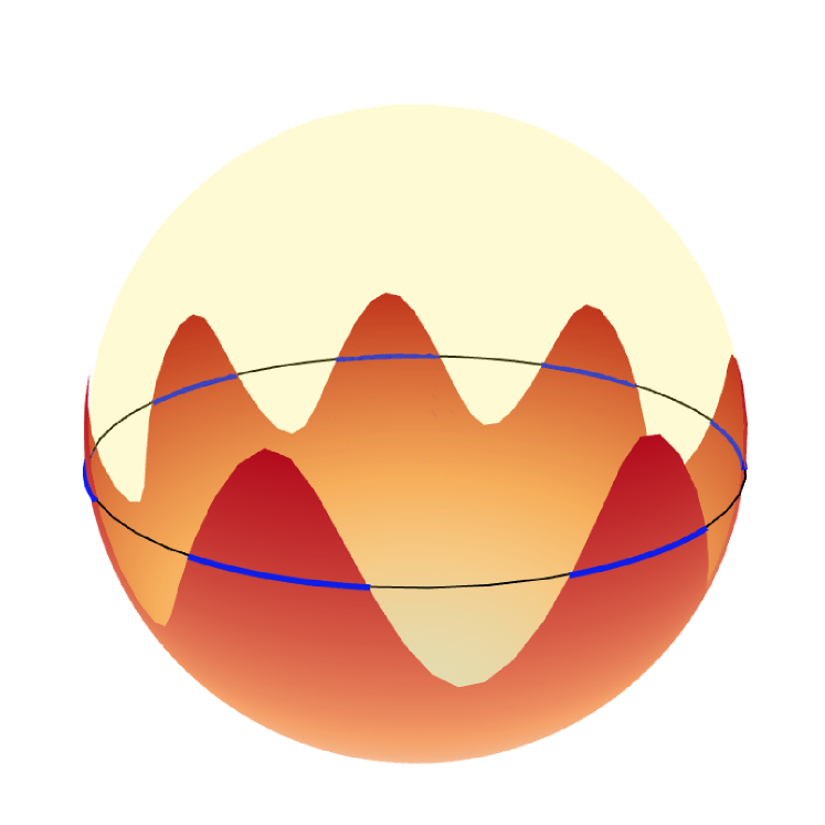
(a) If $L$ is horizontal, then $Z=M\cap L$ is the disjoint union of $7$ segments of circles.

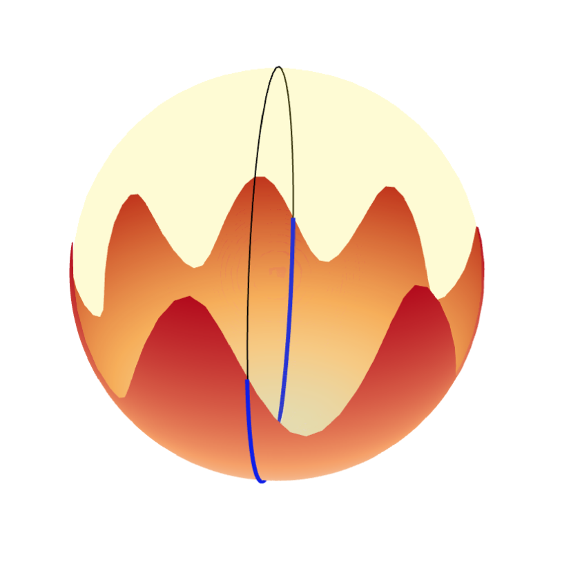
(b) If $L$ is vertical, then $Z=M\cap L$ is a semi-circle.

Figure 1. The pictures shows two nodal lines of the Gaussian field $X=\hat{X}|_{M}$ on the manifold $M:=\left\{(t,re^{i\theta})\in\mathbb{S}^{2}:t\leq\frac{2}{7}\sin(7\theta)\right\}$, where the second entry of the vector $(t,r\theta)$ is expressed in polar coordinates. They both are of the form $Z=M\cap L$, with $L=X^{-1}(0)$ being a plane in $\mathbb{R}^{2}$

The next section contains a discussion of the main methodological innovations established in our work and serves as a plan for the rest of the paper.

1.5. Main technical contributions and structure of the paper

1. Criteria for absolute continuity on Banach spaces. Section 3 contains general criteria — stated in Theorem 3.2 and Corollary 3.4 — ensuring that the distribution of a random variable of the form $V=V(X)$, where $X$ is a Banach space-valued Gaussian random element, is not singular with respect to the Lebesgue measure. Our conditions require, in particular, that the Fréchet differential $d_{f}V$ is not zero for some $f$ in the topological support of the law of $X$. As discussed below, our strategy of proof is close in spirit to the arguments rehearsed in [31].

2. Explicit formulae for differentials of nodal volumes. The main achievement of Section 4 is the following new explicit formula for the differential of nodal volumes. Let $(M,g)$ be a $m$-dimensional $\mathcal{C}^{2}$ Riemannian manifold (possibly with boundary) and let $\mathcal{U}$ denote the open subset of $\mathcal{C}^{2}(M)$ composed of those $f$ having zero as a regular value; then, setting $V(f)=\mathcal{H}^{m-1}(f^{-1}(0))$, one has that $V\in\mathcal{C}^{1}(\mathcal{U})$ and, for all $f\in\mathcal{U}$,

   (1.7) $$\langle d_{f}V,h\rangle=-\int_{Z}h\cdot\frac{\tilde{\Delta}f}{\|df\|^{2}}dZ+\int_{\partial Z}h\cdot\frac{g(\mathbf{n},\nu)}{\|d(f|_{\partial M})\|}d\partial Z,$$

   where $Z:=f^{-1}(0)$, $\nu:=\|\mathrm{grad}f\|^{-1}\mathrm{grad}f$, $\tilde{\Delta}f:=\Delta f-\mathrm{Hess}f(\nu,\nu)$ and the scalar product on the right-hand side corresponds to the duality pairing notation. Formula (1.7) (whose proof is based on classical variational formulae discussed e.g. in [57]) is our main tool for directly applying the absolute continuity criteria discussed above, as well as for studying the Malliavin-Sobolev regularity of nodal volumes. As discussed in Remark 4.1, when specialized to a Euclidean setting (in which $f$ is e.g. a smooth stationary Gaussian field on some rectangle $M$, having zero as a regular value with probability one), relation (1.7) can be formally deduced by differentiating the classical relation

   (1.8) $$\mathcal{H}^{m-1}(f^{-1}(0))=\int_{M}\delta_{0}(f(x))\,\|\nabla\,f(x)\|_{\mathbb{R}^{m}}\,dx,$$

   where the right-hand side of the previous equation has to be regarded as the appropriate limit of integrals where $\delta_{0}$ is replaced by a smooth kernel. See e.g. [29, 61, 62, 73] for a sample of references directly using (or referring to) (1.8). We observe that relation (1.7) is the key in the proof of Proposition 1.5.

3. Transversality of random curves in function spaces. In Section 5, we focus on the characterization of random segments of the form $[X,X+h]:=\{X+th:t\in[0,1]\}$ (as special cases of more general $\mathcal{C}^{2}(M)$-valued curves $\{f_{t}\}$), where $X$ is a smooth Gaussian field satisfying Assumption A and $h$ is a fixed element of the associated Cameron-Martin space. Our main achievement — see Theorem 5.10 — is the proof that a.s. $[X,X+h]$ only intersects transversely the exceptional subset of $\mathcal{C}^{2}(M)$ composed of functions having zero as a critical value, in such a way that the intersections are finite in number and correspond to mappings for which zero is a Morse critical value. Such a result is the key element to verify the property of ray absolute continuity that is necessary to establish the Malliavin-Sobolev regularity of nodal volumes. See Section 5.7 for the appropriate notion of transversality, as well as Theorem 5.12 for some special results needed in the two-dimensional case.

4. Regularity of nodal volumes along transverse curves via a transfer principle. One of the crucial consequences of the findings of Section 5 (see, in particular, Corollary 5.11), is that the study of the local regularity of mappings of the type $t\mapsto V(f_{t})$, where $V$ is the nodal volume and $\{f_{t}\}$ is a transverse curve, can be reduced to the local analysis of functions with the form $t\mapsto V(T-t)$, where $T$ is a Morse mapping on an adequate ancillary manifold with the same dimension. Our analysis (see e.g. Lemmas 6.8 and 6.9) reveals that the local regularity of these mappings strongly depends on the dimension on the manifold $M$. The results of Section 5 and Section 6 are brought together in Section 7, which also contains the proof of the non-singularity of the law of nodal volumes under Assumption A and an additional non-constancy requirement.

5. Malliavin-Sobolev regularity via Kac-Rice formulae. As already discussed, Sections 8 and 9 establish the necessary integrability conditions for nodal volumes, and for the associated norms of weak derivatives, by repeatedly using Kac-Rice formulae – as applied in particular to (1.7). Such an approach has to be contrasted with the techniques developed in [7], where such a task is accomplished through the study of the local regularity of the integrand appearing in an (already evoked) exact Rice formula for nodal volumes.

6. Structure of the law of nodal volumes under a full support assumption. As anticipated, Section 10 contains a full proof of Equation (1.1). In Remark 10.2 it is argued that the main argument in the proof addresses a conjecture formulated in [7, Section 4].

7. Constraints on the index of simultaneous critical points. For a Gaussian field $X$ satisfying Assumption A, the event that a random segment $[X,X+h]$ contains functions $f$ with multiple critical zeros might have positive probability, although Assumption A ensures that all those critical points are Morse. For instance, if $X$ is a periodic function, on the torus $\mathbb{T}^{m}$ or on a domain $D\subset\mathbb{R}^{m}$ with small enough period, we prove (Theorem 5.12) that almost surely, if such event occours, there are precise constraints on the Morse index of the critical points of $f$. It is surprising that this is true under the sole Assumption A, so in particular, without making any assumption on the correlation of the random variables $X(p)$ and $X(q)$ at distinct points $p\neq q\in M$.

8. Negligible events in Gaussian spaces. We signal that Lemma B.3, despite its very technical appearence, provides a very efficient strategy to prove that certain events have zero Gaussian probability, especially those arising from a differential condition, and involving random segments. Indeed, it works when more standard transversality arguments — like those on which Lemma 5.4, Lemma 5.2 (Bulinskaya) and Theorem 5.10 rely on — are not available. It is a key ingredient in the proof of Theorem 5.12 and in the proof of Theorem 10.1, to prove the validity of Equation 1.1 in point (i) of Theorem 1.2.

The forthcoming Section 2 contains a list of preliminary definitions and notational conventions, whereas the formal definition of the Malliavin-Sobolev space $\mathbb{D}^{1,p}$ is deferred to Section 3.2.

1.6. Acknowledgments.

The authors are thankful to J. Angst and G. Poly for useful discussions. This research is supported by the Luxembourg National Research Fund (Grant: 021/16236290/HDSA).

2. Notations

The following list contains some recurring conventions adopted in our work.

1. A random element (see [19]) of the topological space $T$ (or with values in $T$) is a measurable mapping $X\colon\Omega\to T$, defined on $(\Omega,\mathfrak{S},\mathbb{P})$. In this case, one writes

   (2.1) $$X\mathchoice{\raisebox{-1.50696pt}{$\displaystyle{{}^{\subset}}$}\mkern-11.5mu\raisebox{1.93747pt}{$\displaystyle{{}_{\subset}}$}}{\mkern 1.0mu\raisebox{-1.1625pt}{$\textstyle{{}^{\subset}}$}\mkern-11.7mu\raisebox{1.93747pt}{$\textstyle{{}_{\subset}}$}}{\raisebox{1.50696pt}{$\scriptstyle\subset$}\mkern-14.0mu\raisebox{-0.6458pt}{$\scriptstyle\subset$}}{\raisebox{1.29167pt}{$\scriptscriptstyle\subset$}\mkern-13.5mu\raisebox{-0.43057pt}{$\scriptscriptstyle\subset$}}T$$

   and denote by $[X]=\mathbb{P}X^{-1}$ the (push-forward) Borel probability measure on $T$ induced by $X$. We will use the notation

   (2.2) $$\mathbb{P}\{X\in U\}:=\mathbb{P}X^{-1}(U)$$

   to indicate the probability that $X\in U$, for some Borel measurable subset $U\subset T$, and write (as usual)

   (2.3) $$\mathbb{E}\{f(X)\}:=\int_{T}f(t)d[X](t),$$

   to denote the expectation of the random variable $f(X)$, where $f\colon T\to\mathbb{R}^{k}$ is a measurable mapping such that the above integral is well-defined. We will sometimes write that $X$ is a random variable, a random vector or a random mapping, respectively, when $T$ is the real line, a vector space, or a space of functions $\mathcal{C}^{r}(M,N)$, respectively. Finally, if $T_{1}\subset T$ is a measurable subset such that $\mathbb{P}\{X\in T_{1}\}=1$, then we will also write $X\mathchoice{\raisebox{-1.50696pt}{$\displaystyle{{}^{\subset}}$}\mkern-11.5mu\raisebox{1.93747pt}{$\displaystyle{{}_{\subset}}$}}{\mkern 1.0mu\raisebox{-1.1625pt}{$\textstyle{{}^{\subset}}$}\mkern-11.7mu\raisebox{1.93747pt}{$\textstyle{{}_{\subset}}$}}{\raisebox{1.50696pt}{$\scriptstyle\subset$}\mkern-14.0mu\raisebox{-0.6458pt}{$\scriptstyle\subset$}}{\raisebox{1.29167pt}{$\scriptscriptstyle\subset$}\mkern-13.5mu\raisebox{-0.43057pt}{$\scriptscriptstyle\subset$}}T_{1},$ by a slight abuse of notation.

2. The space of $\mathcal{C}^{r}$ functions between two manifolds $M$ and $N$ is denoted by $\mathcal{C}^{r}(M,N)$. We simply write $\mathcal{C}^{r}(M)=\mathcal{C}^{r}(M,\mathbb{R})$ when $N=\mathbb{R}$. If $E\to M$ is a vector bundle, we denote the space of its $\mathcal{C}^{r}$ sections by $\Gamma^{r}(E)$ (see e.g. [48, Chapter 10]). Both spaces $\mathcal{C}^{r}(M,N)$ and $\Gamma^{r}(E)$ are regarded as topological spaces endowed with the weak Whitney’s topology (see [40, p. 34]). In particular, the space of $\mathcal{C}^{r}$ vector fields on $M$ will be denoted by $\mathfrak{X}^{r}(M):=\Gamma^{r}(TM)$.

3. The sentence: “$X$ has the property $\mathcal{P}$ almost surely” (abbreviated “a.s.”) means that the set $S=\{t\in T:t\text{ has the property }\mathcal{P}\}$ contains a Borel set of $[X]$-measure $1$. It follows, in particular, that the set $S$ is $[X]$-measurable, i.e. it belongs to the $\sigma$-algebra obtained from the completion of the measure space $(T,\mathcal{B}(T),[X])$.

4. We write $\#(S)$ for the cardinality of the set $S$.

5. We use the symbol $A\mathrel{\text{\raise-0.43057pt\vbox{ \halign{#\cr\smash{$-$}\crcr$\pitchfork$\crcr} }}}B$ to say that objects $A$ and $B$ are in transverse position, in the usual sense of differential topology (as in [40, p. 74] and Definition 5.3).

3. Absolute Continuity and Differentiability on Banach Spaces

In this section, we use some basic elements of the theory Gaussian measures on Banach spaces. The reader is referred to [21, Chapters 2 and 3] for a comprehensive discussion; see also [39, Section 4] for a succinct presentation. From now on, the notational conventions from Section 2 are adopted without further notice.

3.1. Some general statements

Let $E$ be a Banach space, denote by $E^{*}$ its dual and write $\langle\lambda,g\rangle$, $\lambda\in E^{*},\,g\in E$, to indicate the usual duality pairing. We endow $E$ with a centered Gaussian probability measure $\mu$ (see [21, Definition 2.1]), and we assume that $\mu=[X]$, that is, $X\mathchoice{\raisebox{-1.50696pt}{$\displaystyle{{}^{\subset}}$}\mkern-11.5mu\raisebox{1.93747pt}{$\displaystyle{{}_{\subset}}$}}{\mkern 1.0mu\raisebox{-1.1625pt}{$\textstyle{{}^{\subset}}$}\mkern-11.7mu\raisebox{1.93747pt}{$\textstyle{{}_{\subset}}$}}{\raisebox{1.50696pt}{$\scriptstyle\subset$}\mkern-14.0mu\raisebox{-0.6458pt}{$\scriptstyle\subset$}}{\raisebox{1.29167pt}{$\scriptscriptstyle\subset$}\mkern-13.5mu\raisebox{-0.43057pt}{$\scriptscriptstyle\subset$}}E$ is a random element whose push-forward measure on $E$ coincides with $\mu$ (see Section 2–(ii) and subsequent discussion). Accordingly, we will use the notation $\mathcal{H}_{X}$ to indicate the Cameron-Martin space associated with $\mu$, as defined e.g. in [21, p. 44]. We recall that $\mathcal{H}_{X}$ is a Hilbert space with the properties that the inclusion $\mathcal{H}_{X}\subset E$ is injective and continuous, and the random element $X$ such that $\mu=[X]$ can be chosen in such a way that

(3.1) $$X=\sum_{n\in\mathbb{N}}\gamma_{n}h_{n},$$

for an arbitrary orthonormal Hilbert basis $(h_{n})_{n}$ of $\mathcal{H}_{X}$ and any family $(\gamma_{n})_{n}$ of i.i.d. random variables $\gamma_{n}\sim\mathcal{N}(0,1)$, where the series converges in $E$, a.s.-$\mathbb{P}$. See e.g. [21, Theorem 3.5.1], as well as the forthcoming Remark 3.5, for concrete examples.

In the sequel, we will assume that $\mu$ is non-degenerate, meaning that the topological support of $\mu$ is the whole space $E$, that is: for each open subset $A\subset E$ one has that $\mu(A)>0$ (see e.g. [21, Definition 3.6.2]). According to [21, Theorem 3.6.1], this property is equivalent to the fact that $\mathcal{H}_{X}$ is dense in $E$.

Remark 3.1.

Following e.g. [21, Definition A.3.14], we recall that the topological support of the measure $\mu$ — henceforth written ${\rm supp}(\mu)$ — is defined to be the smallest closed subset of $E$ such that $\mu(\,{\rm supp}(\mu)\,)=1$. Since (again by virtue [21, Theorem 3.6.1]) the set ${\rm supp}(\mu)$ coincides with the closure of $\mathcal{H}_{X}$ in $E$, one can bypass the non-degeneracy assumption on $\mu$ by considering instead the restriction of $\mu$ to the Banach (sub)space ${\rm supp}(\mu)$.

Now fix a Borel measurable mapping $V\colon E\to\mathbb{R}$, and assume that there exists an open subset $\mathcal{U}_{0}\subset E$ such that $V$ is of class $\mathcal{C}^{1}$ on $\mathcal{U}_{0}$, that is, there exists a continuous mapping $dV:\mathcal{U}_{0}\to E^{*}$ such that, as $g\to 0$ in $E$,

(3.2) $$V(f+g)=V(f)+\langle d_{f}V,g\rangle+o\left(\|g\|\right),$$

where we used the duality pairing notation introduced above. The following statement provides a straightforward criterion ensuring that there exists a truncation of the random variable $V(X)$ whose law is absolutely continuous.

Theorem 3.2.

Let the above setting and assumptions prevail (in particular, $X$ is a $E$-valued random element with non-degenerate distribution $\mu$), and assume that $d_{f}V\neq 0$ for some $f\in\mathcal{U}_{0}$. Then, there exists an open neighborhood $\mathcal{O}\subset\mathcal{U}_{0}$ of $f$ such that the law of the random variable $V1_{\mathcal{O}}:=V(X)1_{\mathcal{O}}(X)$ is absolutely continuous with respect to the Lebesgue measure.

Proof.

By density and continuity, we can find $h_{0}\in\mathcal{U}_{0}$ and $h\in\mathcal{H}_{X}$ such that $\langle d_{h_{0}}V,h\rangle\neq 0$. Without loss of generality, we can assume that $|h|=1$. The rest of the proof is partially based on a construction reminiscent of the arguments rehearsed in [31, Section 2]. Define the closed Banach subspace $E_{0}:=\overline{\{h\}^{\perp}}$ (closure of $\{h\}^{\perp}$ in $E$). Then, using e.g. [31, first Lemma of Section 2], one sees that there is a splitting $E=E_{0}\oplus\mathbb{R}h$ such that the random element $X$ can be written as $X=Y+h\gamma$, where $Y\mathchoice{\raisebox{-1.50696pt}{$\displaystyle{{}^{\subset}}$}\mkern-11.5mu\raisebox{1.93747pt}{$\displaystyle{{}_{\subset}}$}}{\mkern 1.0mu\raisebox{-1.1625pt}{$\textstyle{{}^{\subset}}$}\mkern-11.7mu\raisebox{1.93747pt}{$\textstyle{{}_{\subset}}$}}{\raisebox{1.50696pt}{$\scriptstyle\subset$}\mkern-14.0mu\raisebox{-0.6458pt}{$\scriptstyle\subset$}}{\raisebox{1.29167pt}{$\scriptscriptstyle\subset$}\mkern-13.5mu\raisebox{-0.43057pt}{$\scriptscriptstyle\subset$}}E_{0}$ is a Gaussian random element with values in $E_{0}$ (with Cameron-Martin space $\mathcal{H}_{Y}=\{h\}^{\perp}$) and $\gamma\sim\mathcal{N}(0,1)$, in such a way that $Y$ and $\gamma$ are independent. Let $\mathcal{O}:=\mathcal{O}_{0}\oplus(a,b)h$ be an open neighborhood of $h_{0}$ such that $0\notin\{\langle d_{f}V,h\rangle:f\in\mathcal{O}\}$, where $\mathcal{O}_{0}\subset E_{0}$ is open and $a,b\in\mathbb{R}$. For any $g\in\mathcal{O}_{0},$ then, the function $t\mapsto V(g+th)$ is a $\mathcal{C}^{1}$ diffeomorphism between two intervals: $(a,b)\to(V(g+ah),V(g+bh))$, so that, if $Z\subset\mathbb{R}$ has zero Lebesgue measure, then $1_{Z}\left(V(g+th)\right)=0,$ for a.e. $t\in(a,b).$ As a consequence,

(3.3) $$\left(\left(V1_{\mathcal{O}}\right)_{*}\mu\right)\left\{Z\right\} =\mathbb{E}\left\{1_{\mathcal{O}_{0}}(Y)1_{(a,b)}(\gamma)1_{Z}\left(V(Y+\gamma h)\right)\right\}$$

$$=\mathbb{E}\left\{1_{\mathcal{O}_{0}}(Y)\int_{a}^{b}1_{Z}\left(V(Y+th)\right)\rho(t)dt\right\}=0.$$

∎

Remark 3.3.

To keep the notational complexity of the present paper within bounds, in the following we will only deal with Gaussian random elements with values in Banach spaces, so that Theorem 3.2 will be enough for our purposes. One should note, however, that the above-displayed arguments can be made to work in the case where $E$ is a non-complete normed vector space or non-normed Fréchet space.

The following statement is a direct consequence of Theorem 3.2. It is a general criterion allowing one to deduce that the law of a given function of the Gaussian element $X$ has an absolutely continuous component.

Corollary 3.4.

Under the assumptions of this section, consider a mapping $V:E\to\mathbb{R}$ that is differentiable and non-constant on some connected open subset of $E$. Then, the law of the random variable $V(X)$ and the Lebesgue measure are not mutually singular.

Remark 3.5.

Let $M$ be a $\mathcal{C}^{2}$, compact $m$-dimensional manifold. Most of the Banach spaces encountered in the present work will have the form of closed subsets of the class $\mathcal{C}^{2}(M)$, that we endow with the weak Whitney’s topology — see Section 2–(iii). As explained e.g. in [40, p. 35], the set $\mathcal{C}^{2}(M)$ (and therefore any of its closed subsets) can be equipped with the structure of a Banach space. Now consider a centered Gaussian measure $\mu$ on $\mathcal{C}^{2}(M)$, and let $\mu=[X]$ for some random field $X$ with covariance $K_{X}$ (note that, necessarily, $K_{X}\in C^{2,2}(M\times M)$). According e.g. to the discussion contained in [21, Section 2.4] or [53, Section 4 and Appendix A], the Cameron-Martin space $\mathcal{H}_{X}$ admits the following standard characterization:

1. Let $D$ be the linear space generated by the collection of Dirac masses $\{\delta_{p}:p\in M\}$ and define $\mathcal{H}$ to be Hilbert space obtained as the closure of (an appropriate quotient of) $D$ with respect to the bilinear extension of the inner product $\langle\delta_{p},\delta_{q}\rangle=K_{X}(p,q).$ Then, $\mathcal{H}_{X}$ is the subset of $\mathcal{C}^{2}(M)$ given by the mappings $\Phi_{h}:p\mapsto\Phi_{h}(p):=\langle h,\delta_{p}\rangle$, $h\in\mathcal{H}$, with inner product $\langle\Phi_{h},\Phi_{g}\rangle_{\mathcal{H}_{X}}=\langle h,g\rangle$.

2. If $G\in\mathcal{C}^{2}(M)^{*}$ has the form

   $$G(f)=\int_{M}f(p)\,\theta(dp)=\int_{M}\delta_{p}(f)\,\theta(dp),\quad f\in\mathcal{C}^{2}(M),$$

   for some finite signed Borel measure $\theta$, then $G\in\mathcal{H}_{X}^{*}\simeq\mathcal{H}_{X}$ and

   $$\|G\|^{2}_{\mathcal{H}_{X}}=\int_{M}\int_{M}\langle\delta_{p},\delta_{q}\rangle\,\theta(dp)\theta(dq)=\int_{M}\int_{M}K_{X}(p,q)\,\theta(dp)\theta(dq).$$

   A full characterization of $C^{2}(M)^{*}$ (not needed in our work) is provided in [53, Theorem 44].

Several consequences of Corollary 3.4 are discussed in Section 7.3.

3.2. Malliavin-Sobolev spaces

This is the right place for introducing the Malliavin-Sobolev spaces $\mathbb{D}^{1,p},$ for all $p\geq 1$. The next definition corresponds to the content of [21, Definitions 5.2.3 and 5.2.4], with one exception: at Point (i) below, we decided to state the property of “ray absolute continuity” in a form that is more suitable for the framework of our paper. For the sake of completeness, the equivalence between the two formulations is proved in Appendix A. Finally, to be in line with the notation adopted in the standard references [75, Section 1.2] and [72, Section 2.3], we use the symbol $\mathbb{D}^{1,p}(\mu)$ instead of writing $\mathbb{D}^{p,1}(\mu)$ (inverting $1,p$ to $p,1$) as in [21].

Definition 3.6.

Let $E$ be a Banach space equipped with a centered Gaussian measure $\mu=[X]$ having full support, and let $\mathcal{H}_{X}\subset E$ be the associated Cameron-Martin Hilbert space. Let $1\leq p<\infty.$ We write $\mathbb{D}^{1,p}(\mu)$ to indicate the Malliavin-Sobolev space of all functions $V\in L^{p}(\mu),$ with the following properties:

1. ($V$ is ray absolutely continuous) For every $h\in\mathcal{H}_{X},$ there is a measurable set $N_{h}\subset E,$ with $\mu(N_{h})=0,$ such that for all $x\in E\smallsetminus N_{h},$ the function $t\mapsto V(x+th)$ coincides $dt$-almost everywhere with an absolutely continuous function $t\mapsto\varphi(t)$.

2. ($V$ is stochastically Fréchet differentiable) There exists measurable mapping

   $${\mathrm{D}_{\mathscr{M}}V:E\to\mathcal{H}_{X}^{*}}$$

   such that for any $h\in\mathcal{H}_{X},$ the expression

   (3.4) $$\mu\left\{x\in E\colon\left|\frac{V(x+th)-V(x)}{t}-\langle\mathrm{D}_{\mathscr{M}}V(x),h\rangle\right|>\varepsilon\right\}$$

   tends to zero as $t\to 0,$ for any choice of $\varepsilon>0$, i.e., there is convergence in probability of the divided difference. The mapping $\mathrm{D}_{\mathscr{M}}V$ is called the stochastic derivative of $V.$

3. The stochastic derivative is $p$-integrable: $\mathbb{E}\|\mathrm{D}_{\mathscr{M}}V\|_{\mathcal{H}_{X}}^{p}<\infty.$

If $V\in\mathbb{D}^{1,p}(\mu),$ then the random variable $\mathrm{D}_{\mathscr{M}}V(X)\mathchoice{\raisebox{-1.50696pt}{$\displaystyle{{}^{\subset}}$}\mkern-11.5mu\raisebox{1.93747pt}{$\displaystyle{{}_{\subset}}$}}{\mkern 1.0mu\raisebox{-1.1625pt}{$\textstyle{{}^{\subset}}$}\mkern-11.7mu\raisebox{1.93747pt}{$\textstyle{{}_{\subset}}$}}{\raisebox{1.50696pt}{$\scriptstyle\subset$}\mkern-14.0mu\raisebox{-0.6458pt}{$\scriptstyle\subset$}}{\raisebox{1.29167pt}{$\scriptscriptstyle\subset$}\mkern-13.5mu\raisebox{-0.43057pt}{$\scriptscriptstyle\subset$}}\mathcal{H}_{X}^{*}$ is called the Malliavin derivative of $V$, and $V$ is said to be in the domain of the Malliavin derivative. We equip $\mathbb{D}^{1,p}(\mu)$ with the norm:

(3.5) $$\|V\|_{\mathbb{D}^{1,p}}:=\mathbb{E}\left\{|V|^{p}\right\}^{\frac{1}{p}}+\mathbb{E}\left\{\|\mathrm{D}_{\mathscr{M}}V\|_{\mathcal{H}_{X}}^{p}\right\}^{\frac{1}{p}}.$$

Remark 3.7.

It is clear from the above definition that if $V\in\mathbb{D}^{1,p}(\mu)$ and $V$ is of class $\mathcal{C}^{1}$ on an open subset $\mathcal{U}\subset E,$ then for $\mu$-a.e. $x\in\mathcal{U}$ one has that

(3.6) $$\mathrm{D}_{\mathscr{M}}V(x)=d_{x}V|_{\mathcal{H}_{X}}.$$

We recall that $\mathcal{H}_{X}$ is continuously embedded in $E$.

Remark 3.8.

By [21, Thm. 5.7.2], the normed spaces $\mathbb{D}^{1,p}(\mu)$ defined above are complete and contain the subset of smooth cylindrical functions as a dense subset, where the smooth cylindrical functions $V\colon E\to\mathbb{R}$ are those of the form $V=F\circ L,$ where $L:E\to\mathbb{R}^{N}$ is a continuous linear map for some $N\in\mathbb{N}$ and $F\in\mathcal{C}^{\infty}(\mathbb{R}^{N})$ has bounded derivatives of all orders. Thus, Definition 3.6 coincides with the most common definition of the Malliavin Sobolev spaces $\mathbb{D}^{1,p}(\mu)$ as the completion of the spaces of smooth cylindrical functions with respect to the norm $\|\cdot\|_{\mathbb{D}^{1,p}}.$ See e.g. [75, Section 1.2] and [72, Section 2.3].

4. Nodal Volumes as Differentiable Mappings: Proof of (1.7)

4.1. Some heuristic considerations

The main achievement of the present section is the derivation of formula (1.7) (see Theorem 4.6). Such a result yields an explicit representation of the Fréchet differential $d_{f}V$ (as defined in (3.2)) in the case where $E$ is a closed subset of the space $\mathcal{C}^{2}(M)$ associated with a $m$-dimensional compact $\mathcal{C}^{2}$ Riemannian manifold $M$, and $V(f)=\mathcal{H}^{m-1}(f^{-1}(0))$ is the nodal volume of a mapping $f\in\mathcal{C}^{2}(M)$ such that $0$ is a regular value of $f$ (see Definitions 4.2 and 4.3).

Remark 4.1.

Fix $m\geq 2$. In the case where $M$ is a bounded domain of $\mathbb{R}^{m}$ with a smooth boundary, and $f:M\rightarrow\mathbb{R}$ is a $\mathcal{C}^{2}$ mapping such that $0$ is a regular value of $f$, formula (1.7) takes the following simple form: for the mapping $g\mapsto V(g)=\mathcal{H}^{m-1}(g^{-1}(0))$ and for any $h\in\mathcal{C}^{2}(M)$, writing $Z=f^{-1}(0)$, one has that

$$\langle d_{f}V,h\rangle = \int_{Z}\frac{h(x)}{\|\nabla f(x)\|^{2}}\cdot\left\{\nu\,{\rm Hess}f(x)\nu^{T}-\Delta f(x)\right\}\,\mathcal{H}^{m-1}(dx)$$

$$+\int_{Z\cap\partial M}h(x)\cdot\frac{\langle\nabla f(x),{\bf n}(x)\rangle}{\|\nabla(f|_{\partial M})\|\|\nabla f(x)\|}\mathcal{H}^{m-2}(dx),$$

where $\nu=\nabla\,f(x)/\|\nabla\,f(x)\|$, and ${\bf n}(x)$ is the outward pointing normal at $x\in\partial M$. It is interesting that formula (4.1) can be deduced by formally differentiating the right-hand side of (1.8) under the integral sign. Writing $A_{x}(g):=\delta_{0}(g(x))$ and $B_{x}(g):=\|\nabla g(x)\|$, one has indeed the formal chain rule

(4.2) $$\langle d_{f}V,h\rangle = \int_{M}\langle d_{f}A_{x},h\rangle\|\nabla f(x)\|dx+\int_{M}\delta_{0}(f(x))\langle d_{f}B_{x},h\rangle dx:=(I)+(II).$$

Now, standard computations yield that

$$\langle d_{f}B_{x},h\rangle=\frac{\langle\nabla f(x),\nabla h(x)\rangle}{\|\nabla f(x)\|},$$

whereas a formal integration by parts based on the divergence theorem leads to

$$(I)=-\int_{M}\delta_{0}(f(x))\left\{\nabla\bullet\frac{h(x)\nabla f(x)}{\|\nabla f(x)\|}\right\}dx+\int_{\partial M}\delta_{0}(f(x))h(x)\frac{\langle\nabla f(x),{\bf n}(x)\rangle}{\|\nabla f(x)\|}dx,$$

where the symbol $\bullet$ indicates a scalar product in $\mathbb{R}^{m}$; the fact that $(I)+(II)$ equals the right-hand side of (4.1) now follows by explicitly computing the term between curly brackets inside the first integral.

4.2. Elements of Riemannian geometry

Our main references for this section are the monographs [2, 40, 48, 49, 57], to which we refer the reader for any unexplained notion and results. For $m\geq 1$, we consider an $m\geq 1$ dimensional $\mathcal{C}^{2}$ compact Riemannian manifold $M$, possibly with boundary $\partial M$, endowed with a metric $g:TM\otimes TM\to\mathbb{R}$ of class $\mathcal{C}^{2}$, with associated norm $\|\cdot\|=\sqrt{g(\cdot,\cdot)}$. We can think that $M$ is a stratified manifold (see [2, Section 8.1]) with two strata: the interior ${\kern 0.0ptM}^{\mathrm{o}}$ of dimension $m=:\dim M$ and the boundary $\partial M$ of dimension $m-1$, with the tangent bundle of ${\kern 0.0ptM}^{\mathrm{o}}$ that extends to a vector bundle $TM$ over all $M$. There is a $\mathcal{C}^{1}$ section $\mathbf{n}:\partial M\to TM$ defined as the unit (i.e., $\|\mathbf{n}\|=1$) outward normal vector to $\partial M$, so that $TM|_{\partial M}=T{\partial M}\oplus_{\perp}\mathrm{span}\{\mathbf{n}\}$; see e.g. [48, p. 391].

4.2.1. Volumes

We use the notation $\int_{M}fdM=\int_{M}f(p)dM(p)$ for the integration of a Borel function $f:M\to\mathbb{R}$ with respect to the volume measure of $(M,g)$. The integral is defined as the linear functional such that when $f$ is supported in the domain of a chart $\varphi\colon O\to\mathbb{R}^{m}$,

(4.3) $$\int_{M}fdM:=\int_{\varphi(O)}f(\varphi^{-1}(x))\sqrt{\det G(x)}dx,$$

where $G_{ij}(x)=g\left(\frac{\partial\varphi^{-1}}{\partial x^{i}}(x),\frac{\partial\varphi^{-1}}{\partial x^{j}}(x)\right)$. In particular, if $Z\subset M$ is a submanifold of dimension $k$, endowed with the metric induced by $g$ and $\operatorname{\mathcal{H}}^{k}$ denotes the $k$-dimensional Hausdorff measure on $M$ with respect to the geodesic distance induced by $g$ (see e.g. [2, pp. 168-169]), then $\int_{Z}fdZ=\int_{M}f(p)1_{Z}(p)\operatorname{\mathcal{H}}^{k}(dp)$, so that the volume, or $k$-volume, of $Z$ is

(4.4) $$\operatorname{\mathcal{H}}^{k}(Z)=\int_{Z}1dZ.$$

Plainly, the $1$-volume is the length and the $2$-volume is the surface area.

4.2.2. Gradient, Hessian and Laplacian

The metric induces an isomorphism of vector bundles $\sharp_{g}\colon T^{*}M\to TM$, which raises the indices and whose inverse is denoted by $\flat_{g}$. We will adopt the standard notation

(4.5) $$\alpha^{\sharp}:=\sharp_{g}(\alpha),$$

for any $\alpha\in T^{*}_{p}M$, so that for all $v\in T_{p}M$, we have $g(\alpha^{\sharp},v)=\langle\alpha,v\rangle$. The gradient of a differentiable function $f\in\mathcal{C}^{2}(M)$ is the vector field $\mathrm{grad}{f}={df}^{\sharp}\in\mathfrak{X}^{1}(M)$ such that

(4.6) $$g\left(\mathrm{grad}f(p),v\right)=\langle d_{p}f,v\rangle$$

Let $\nabla$ denotes the Levi-Civita connection of the metric $g$. The Hessian of $f\in\mathcal{C}^{2}(M)$ at $p\in M$ is the symmetric bilinear form $\mathrm{Hess}_{p}f\colon T_{p}M\times T_{p}M\to\mathbb{R}$ such that

(4.7) $$\mathrm{Hess}_{p}f(v,w)=\langle\nabla_{v}(d_{p}f),w\rangle,$$

and defines a continuous tensor $\mathrm{Hess}f$. The corresponding linear operator is $\mathrm{H}{\mathrm{ess}}^{\sharp}f=\sharp_{g}\circ\mathrm{Hess}f\colon TM\to TM$, that is the operator such that $g(\mathrm{H}{\mathrm{ess}}^{\sharp}f(v),w)=\mathrm{Hess}f(v,w)$ for all $v,w\in TM$. Since $\nabla\sharp_{g}=\sharp_{g}\nabla,$ it follows that $\mathrm{H}{\mathrm{ess}}^{\sharp}f=\nabla\mathrm{grad}f.$ Taking the trace of the Hessian, with respect to the metric, one obtains the Laplace-Beltrami operator $\Delta\colon\mathcal{C}^{2}(M)\to\mathcal{C}^{0}(M)$, or just the Laplacian, of the metric $g$:

(4.8) $$\Delta f=\mathrm{tr}_{g}(\mathrm{Hess}f)=\mathrm{tr}(\mathrm{H}{\mathrm{ess}}^{\sharp}f).$$

4.2.3. Mean curvature

Given $f\in\mathcal{C}^{2}(M)$, such that $\{p\in M:f(p)=0,d_{p}f=0\}=\emptyset$, then $Z=f^{-1}(0)$ is a $\mathcal{C}^{2}$ hypersurface, cooriented by the normal vector field $\nu=\|\mathrm{grad}f\|^{-1}\mathrm{grad}f$. The second fundamental form of $Z$ at $p\in Z$ is the bilinear form $\mathrm{II}_{p}=\|d_{p}f\|^{-1}\mathrm{Hess}_{p}f|_{TZ}$. Indeed, for any $v,w\in T_{p}Z$ we have

(4.9) $$\mathrm{II}(v,w)\overset{\mathrm{def}}{=}g(v,\nabla_{w}\nu)=\frac{\mathrm{Hess}f(v,w)}{\|df\|}-g(v,\nu)\frac{\mathrm{Hess}f(\nu,w)}{\|df\|},$$

but the second term vanishes because $T_{p}Z=\nu(p)^{\perp}.$ Finally, the mean curvature of $Z$ is the trace of $\mathrm{II}$ with respect to the restriction of $g$ to $TZ$, that is the function $H_{Z}\in\mathcal{C}^{0}(Z)$

(4.10) $$H_{Z}=\text{tr}_{g}\left({\mathrm{II}}\right)=\|df\|^{-1}\left(\Delta f-\mathrm{Hess}f(\nu,\nu)\right).$$

4.3. Nodal volume and regular values: main results

The next definition formally introduces the main object of our paper.

Definition 4.2 (Nodal volumes).

Let the above notation and assumptions prevail. We define the nodal volume as the mapping $V\colon\mathcal{C}^{2}(M)\to\mathbb{R}\,\colon f\mapsto V(f)$ such that

(4.11) $$V(f):=\operatorname{\mathcal{H}}^{m-1}(f^{-1}(0)).$$

Observe that the definition of $V$ is well given because $f^{-1}(0)$ is a closed (and, therefore, Borel) set. In general, $V$ is a mapping possessing some degree of regularity only when restricted to functions $f$ such that $f^{-1}(0)$ is a submanifold – the latter property is encoded in the fundamental notion of regular value.

Definition 4.3 (Regular Values).

For $m\geq 1$, let $M$ be a $m$-dimensional $\mathcal{C}^{2}$ Riemannian manifold with boundary, let $f\in\mathcal{C}^{2}(M)$ and $r\in\mathbb{R}$. If $\partial M=\emptyset$, then we say that $r$ is a regular value of $f$, and write $f\mathrel{\text{\raise-0.43057pt\vbox{ \halign{#\cr\smash{$-$}\crcr$\pitchfork$\crcr} }}}r$, if for every $p\in M$, the following implication holds: $f(p)=r\implies d_{p}f\neq 0$. In general, we say that $r$ is a regular value of $f$, and write $f\mathrel{\text{\raise-0.43057pt\vbox{ \halign{#\cr\smash{$-$}\crcr$\pitchfork$\crcr} }}}r$, if and only if $f|_{{\kern 0.0ptM}^{\mathrm{o}}}\mathrel{\text{\raise-0.43057pt\vbox{ \halign{#\cr\smash{$-$}\crcr$\pitchfork$\crcr} }}}r$ and $f|_{\partial M}\mathrel{\text{\raise-0.43057pt\vbox{ \halign{#\cr\smash{$-$}\crcr$\pitchfork$\crcr} }}}r$. Moreover, $r$ is said to be a critical value of $f$ if it is not a regular value. From now on, we write

(4.12) $$\mathcal{U}:=\left\{f\in\mathcal{C}^{2}(M):f\mathrel{\text{\raise-0.43057pt\vbox{ \halign{#\cr\smash{$-$}\crcr$\pitchfork$\crcr} }}}0\right\}.$$

Definition 4.4 (Neat Hypersurfaces).

Following [40, Section 1.4], we say that a subset $Z\subset M$ is a $\mathcal{C}^{2}$ neat submanifold of $M$, having codimension $k$, if for every point $p\in Z$, there is a $\mathcal{C}^{2}$ chart $\varphi\colon O\to\mathbb{R}^{m-1}\times[0,+\infty)$ of $M$ around $p$, such that $Z\cap O=\varphi^{-1}(\mathbb{R}^{m-k})$. As customary, we will say: hypersurface, in place of: submanifold of codimension one.

In particular, a $\mathcal{C}^{2}$ neat hypersurface $Z\subset M$ is a $\mathcal{C}^{2}$ manifold with boundary $\partial Z=Z\cap\partial M$, and such that for every $x\in\partial Z$, we have $T_{x}Z\cap T_{x}\partial M=T_{x}\partial Z$. We refer to [40, Section 1.4] for more details. The following statement explains the relation between the two above definitions; its proofs can be found in [40, Theorem 1.4.1].

Proposition 4.5.

The class $\mathcal{U}$ defined in (4.12) is an open subset of $\mathcal{C}^{2}(M)$. Moreover, if $f\in\mathcal{U}$, then $Z:=f^{-1}(0)$ is a $\mathcal{C}^{2}$ neat hypersurface of $M$.

In short, all subsets that are not neat hypersurfaces are somewhat degenerate for our study. In this sense, the functions in the class $\mathcal{U}$ are non-degenerate, in that the equation $f=0$ defines a neat hypersurface. The next result is the main achievement of the section, as well as the linchpin of the entire paper. The proof is deferred to Section 4.6.

Theorem 4.6 (Nodal volumes as differentiable mappings).

Assume that $M$ is a $\mathcal{C}^{2}$ Riemannian manifold with boundary $\partial M$ and let $\mathbf{n}\in\Gamma^{\infty}(TM|_{\partial M})$ denote the outward normal vector to the boundary. Define $\mathcal{U}\subset\mathcal{C}^{2}(M)$ as in (4.12). Then, the following conclusions hold:

1. The nodal volume mapping $V$ defined in (4.11) is such that $V\in\mathcal{C}^{1}(\mathcal{U})$.

2. Fix $f\in\mathcal{U}$, let $Z:=f^{-1}(0)$, and define $\nu:=\|\mathrm{grad}f\|^{-1}\mathrm{grad}f$ and $\tilde{\Delta}f:=\Delta f-\mathrm{Hess}f(\nu,\nu)$. Then, formula (1.7) holds for all $h\in\mathcal{C}^{2}(M)$, that is:

   (4.13) $$\langle d_{f}V,h\rangle=-\int_{Z}h\cdot\frac{\tilde{\Delta}f}{\|df\|^{2}}dZ+\int_{\partial Z}h\cdot\frac{g(\mathbf{n},\nu)}{\|d(f|_{\partial M})\|}d\partial Z,$$

   where the existence of the integrals on the right-hand side is part of the conclusion.

For the next statement, we assume that $X\mathchoice{\raisebox{-1.50696pt}{$\displaystyle{{}^{\subset}}$}\mkern-11.5mu\raisebox{1.93747pt}{$\displaystyle{{}_{\subset}}$}}{\mkern 1.0mu\raisebox{-1.1625pt}{$\textstyle{{}^{\subset}}$}\mkern-11.7mu\raisebox{1.93747pt}{$\textstyle{{}_{\subset}}$}}{\raisebox{1.50696pt}{$\scriptstyle\subset$}\mkern-14.0mu\raisebox{-0.6458pt}{$\scriptstyle\subset$}}{\raisebox{1.29167pt}{$\scriptscriptstyle\subset$}\mkern-13.5mu\raisebox{-0.43057pt}{$\scriptscriptstyle\subset$}}\mathcal{C}^{2}(M)$ is a centered Gaussian element with values in $\mathcal{C}^{2}(M)$ and law $\mu$. We write $\mathbb{E}[X(p)X(q)]:=K_{X}(p,q)$ for the covariance of $X$ and denote by $E\subset\mathcal{C}^{2}(M)$ the topological support of $\mu$.

Corollary 4.7 (Cameron-Martin norms).

Under the above notation and assumptions, let $\mathcal{H}_{X}\subset E$ denote the Cameron-Martin space of $X$, and assume that

$$\mathbb{P}[X\in\mathcal{U}]=\mu(E\cap\mathcal{U})=1.$$

Let $Z=Z_{X}=X^{-1}(0)$ and set $\nu=\nu_{X}=\|\mathrm{grad}X\|^{-1}\mathrm{grad}X$. Then, the nodal volume mapping $V$ defined in (4.11) is such that $V\in\mathcal{C}^{1}(\mathcal{U}_{0})$, where $\mathcal{U}_{0}:=E\cap\mathcal{U}$, and consequently $d_{X}V|_{\mathcal{H}_{X}}\mathchoice{\raisebox{-1.50696pt}{$\displaystyle{{}^{\subset}}$}\mkern-11.5mu\raisebox{1.93747pt}{$\displaystyle{{}_{\subset}}$}}{\mkern 1.0mu\raisebox{-1.1625pt}{$\textstyle{{}^{\subset}}$}\mkern-11.7mu\raisebox{1.93747pt}{$\textstyle{{}_{\subset}}$}}{\raisebox{1.50696pt}{$\scriptstyle\subset$}\mkern-14.0mu\raisebox{-0.6458pt}{$\scriptstyle\subset$}}{\raisebox{1.29167pt}{$\scriptscriptstyle\subset$}\mkern-13.5mu\raisebox{-0.43057pt}{$\scriptscriptstyle\subset$}}\mathcal{H}_{X}^{*}\cong\mathcal{H}_{X}$. Moreover, a.s.-$\mathbb{P}$,

(4.14) $$\|d_{X}V\|^{2}_{\mathcal{H}_{X}}= \int_{Z}\int_{Z}\frac{\tilde{\Delta}X(p)}{\|d_{p}X\|^{2}}\frac{\tilde{\Delta}X(q)}{\|d_{q}X\|^{2}}K_{X}(p,q)dZ(p)dZ(q)$$

$$+\int_{\partial Z}\int_{\partial Z}\frac{g_{p}(\mathbf{n},\nu)g_{q}(\mathbf{n},\nu)}{\|d_{p}(X|_{\partial M})\|\|d_{q}(X|_{\partial M})\|}K_{X}(p,q)d\partial Z(p)d\partial Z(q).$$

Proof.

The proof is a direct consequence of the content of Remark (3.5)-(b), in the special case $G=d_{X}V$ and $\theta(dp)=\|d_{p}X\|^{-2}1_{Z}(p)dZ+1_{\partial Z}(p)g_{p}(\mathbf{n},\nu)\|d_{p}X|_{\partial M}\|^{-1}d\partial Z$.

∎

Remark 4.8.

In the previous statement, the random element $\Omega\ni\omega\mapsto d_{X}V(\omega)$ is defined as follows: $d_{X}V(\omega)=d_{X(\omega)}V$, whenever $\omega$ is such that $X(\omega)\in\mathcal{U}_{0}$, and $d_{X}V(\omega)=0$ otherwise.

Before proving Theorem 4.6 in Section 4.6, one needs to study in some detail the first-order variations of nodal volumes. The necessary technical statements are gathered together in Sections 4.4 and 4.5.

4.4. First variation of the volume

The mean curvature of a (compact and oriented) hypersurface is known to be the derivative of the $d-1$ dimensional volume of the surface (see [57]), in the sense that if we move $Z$ in the direction of $\nu$ for a small time $t$ inside a closed manifold $M$, then, the volume varies as $\operatorname{\mathcal{H}}^{m-1}(Z_{t})=t\int_{Z}H_{Z}dZ+o(t).$ Let us report the most general formula, including the case when the variation has a tangential component $T\in\mathfrak{X}^{1}(Z)$ and $Z\subset M$ is a submanifold with boundary $\partial Z$ without any assumption on the relative positions of $\partial Z$ and $\partial M$. Assume that $Z_{t}=\phi_{t}(Z)$, where $\phi\colon(-\varepsilon,\varepsilon)\times Z\to M$ is a $\mathcal{C}^{1}$ map such that $\phi_{t}=\phi(t,\cdot)$ is an immersion for all $t$. Let us define the first variation of such family of parametrized hypersurfaces as $\delta{Z}:=\frac{d\phi_{t}}{dt}\big{|}_{t=0}$, which is a $\mathcal{C}^{1}$ section of $TM|_{Z}$. Then we can decompose $\delta Z=T+\dot{Z}\nu$ into a tangential vector field $T\in\mathfrak{X}^{1}(Z)$ and a section of the normal bundle determined by a function $\dot{Z}\in\mathcal{C}^{1}(Z)$. Recall that in this case $T_{z}Z^{\perp}$ is just a line spanned by $\nu(z)=\|\mathrm{grad}f(z)\|^{-1}\mathrm{grad}f(z)$. The following formula holds (see [57, Section 1, page 4]).

(4.15) $$\frac{d}{dt}\Big{|}_{0}\operatorname{\mathcal{H}}_{m-1}\left(Z_{t}\right)=\int_{Z}\dot{Z}\cdot H_{Z}+\mathrm{div}(T)dZ.$$

We will need the following formulation of the above formula.

Proposition 4.9.

Let the assumptions above prevail. If, moreover, $\partial Z_{t}\subset\partial M$, but $TZ_{0}|_{\partial Z_{0}}\neq T\partial M$, then

(4.16) $$\frac{d}{dt}\Big{|}_{0}\operatorname{\mathcal{H}}_{m-1}\left(Z_{t}\right) =\int_{Z}g(\delta{Z},\nu)\cdot H_{Z}dZ-\int_{\partial Z}g(\delta{Z},\nu)\frac{g(\mathbf{n},\nu)}{\sqrt{1-g(\mathbf{n},\nu)^{2}}}d\partial Z,$$

where $H_{Z}$ is the mean curvature of $Z$ in the direction $\nu$, defined as in Equation 4.10.

Proof.

By (4.15) and Stokes-divergence theorem, we have that

(4.17) $$\frac{d}{dt}\Big{|}_{0}\operatorname{\mathcal{H}}_{m-1}\left(Z_{t}\right) =\int_{Z}g(\delta{Z},\nu)\cdot H_{Z}dZ+\int_{\partial Z}g(\mathbf{n}_{\partial},T)d\partial Z,$$

where $\mathbf{n}_{\partial}\in\Gamma^{\infty}(N\partial Z)$ is the outward unit normal vector of $\partial Z$. We have that for $x\in\partial Z$, $\mathbf{n}=\mathbf{n}(x)$ belongs to the space $(T_{x}\partial Z)^{\perp}$ spanned by the orthonormal basis given by $\mathbf{n}_{\partial}=\mathbf{n}_{\partial}(x)$ and $\nu=\nu(x)$, Moreover, by construction, both $\mathbf{n}_{\partial}$ and $\mathbf{n}$ are pointing outside of $\partial M$, thus $g(\mathbf{n},\mathbf{n}_{\partial})=\sqrt{1-g(\mathbf{n},\nu)^{2}}>0$. Under the hypothesis that $\partial Z_{t}\subset\partial M$ for all $t$, we must have that $\delta Z(x)\in T_{x}\partial M=\mathbf{n}^{\perp}$, so that, evaluating at $x$,

(4.18) $$g(\mathbf{n}_{\partial},T)=g(\mathbf{n}_{\partial},\delta Z)=-\frac{g(\mathbf{n},\nu)}{\sqrt{1-g(\mathbf{n},\nu)^{2}}}g(\nu,\delta Z).$$

∎

4.5. Change of variation formula

Let $f\in\mathcal{U}\subset\mathcal{C}^{2}(M)$ and $Z=f^{-1}(0)$. In order to apply the formula of Proposition 4.9 we need to represent the family of hypersurfaces $Z_{t}=(f+th)^{-1}(0)$ as a small translation of $Z$ in the direction of a vector field $\delta Z:Z\to TM$. To this end we look for a time dependent vector field $W\in\mathcal{C}^{1}(\mathbb{R}\times M,TM)$ such that, if $P^{t}$ is the flow of $W_{t}$, then $P^{t}(Z)=Z_{t}$. This is equivalent to look for a solution $W_{t}$ of the equation:

(4.19) $$(f+th)(P^{t}(z))=0,$$

By differentiating with respect to $t$, we get the equivalent condition that:

(4.20) $$\langle d_{p}f+td_{p}h,W_{t}(p)\rangle+h(p)=0,\text{ for all $p\in Z_{t}$ and $t\in(-\varepsilon,\varepsilon)$}.$$

The second equation is solved in a neighborhood of $Z$ by the vector field

(4.21) $$W_{t}=-h\|\mathrm{grad}(f+th)\|^{-2}\mathrm{grad}(f+th),$$

which is of class $\mathcal{C}^{1}$ in that neighborhood. Using a partition of unity, $W_{t}$ can be extended to a $\mathcal{C}^{1}$ vector field $W_{t}$ on the whole manifold $M$. If the manifold is closed, i.e. $\partial M=\emptyset$, then $P^{t}$ is defined for all times and we have $P^{t}(Z)=Z_{t}$ for small enough $t$. In this case, we can apply Proposition 4.9 directly with

(4.22) $$\delta{Z}=W_{0}|_{Z}=-h\frac{\mathrm{grad}f}{\|\mathrm{grad}f\|^{2}}.$$

and deduce the formula for $d_{f}V$ from Equation 4.10. In the general case, we cannot argue that $Z_{t}=P_{t}(Z)$ because the flow $P_{t}$ is not defined for all times, since the trajectories could fall outside the boundary. In this case however, Equation 4.20 holds.

Lemma 4.10.

Let $f\in\mathcal{U}\subset\mathcal{C}^{2}(M)$ and $Z=f^{-1}(0)$. Let $P(t,x)=P^{t}(x)$ be the flow of a time dependent vector field $W\in\mathcal{C}^{1}(\mathbb{R}\times M,TM)$, that satisfies $\eqref{eq:Wt}$ and $g(\mathbf{n},W_{t}|_{\partial M})=0$ for $|t|\leq\varepsilon$. Then, $P:(-\varepsilon,\varepsilon)\times M\to M$ is a $\mathcal{C}^{1}$ map and, for all $t\in(-\varepsilon,\varepsilon)$, the map $P^{t}\colon M\to M$ is a $\mathcal{C}^{1}$ diffeomorphism such that $P^{t}(Z)=Z_{t}$.

Proof.

Since $g(\mathbf{n},W^{\partial}_{t})=0$, the vector field $W_{t}^{n}$ is tangent to the boundary $\partial M$. This ensures, by standard O.D.E. theory (see [40, Section 6.2]), that there exists a flow $P_{t}^{n}\colon M\to M$ of $W_{t}^{n}$ defined for all times $t\in\mathbb{R}$. Since $W^{n}\in\mathcal{C}^{1}(\mathbb{R}\times M,TM)$, by the property of smooth dependence on initial data of O.D.E., we have $P^{n}\in\mathcal{C}^{1}(\mathbb{R}\times M,M)$. ∎

4.6. Proof of Theorem 4.6

Let $Z_{t}=\{f+th=0\}$ and $Z_{0}=Z$. We take the time-dependent vector field ${\kern 0.0ptW}^{\mathrm{o}}_{t}\in\mathcal{C}^{1}(\mathbb{R}\times M,TM)$ is defined so that ${\kern 0.0ptW}^{\mathrm{o}}_{t}=-h\|\mathrm{grad}(f+th)\|^{-2}\mathrm{grad}(f+th)$ in a neighborhood $\mathcal{Q}$ of $Z$ which contains all $Z_{t}$ for $|t|\leq t_{0}$ small enough. Therefore, for every $p\in Z_{t}$, we have that

(4.23) $$\langle d_{p}f+td_{p}h,{\kern 0.0ptW}^{\mathrm{o}}_{t}(p)\rangle+h(p)=0,\text{ for all $p\in Z_{t}$}.$$

Observe that, applying the same argument to $f|_{\partial M}$ yields a time-dependant vector field $W^{\partial}\in\mathcal{C}^{1}(\partial M\times\mathbb{R},T\partial M)$ such that

(4.24) $$\langle d_{p}f+td_{p}h,W^{\partial}_{t}(p)\rangle+h(p)=0,\text{ for all $p\in\partial Z_{t}$}.$$

Let $\rho_{n}\in\mathcal{C}^{\infty}(M,[0,1])$ be a sequence of smooth functions such that $\rho_{n}(\partial M)=1$ and such that $\sup_{K}\rho_{n}\to_{n\to\infty}0$ for any $K\subset{\kern 0.0ptM}^{\mathrm{o}}$ compact subset. This can be achieved by taking $\rho_{n}$ supported in a tubular neighborhood of $\partial M$ of radius $\frac{1}{n}$. It is also convenient to extend $\mathbf{n}$ and $W^{\partial}_{t}$ to vector fields $\mathbf{n}\in\mathfrak{X}^{\infty}(M)$ and $W^{\partial}_{t}\in\mathfrak{X}^{1}(M)$. We can assume that Equation 4.24 remains true for all $p$ in a fixed neighborhood $\mathcal{Q}_{\partial}$ containing $\partial Z_{t}$ for all $|t|\leq t_{0}$. Define

(4.25) $$W_{t}^{n}:={\kern 0.0ptW}^{\mathrm{o}}_{t}(1-\rho_{n})+W^{\partial}_{t}\rho_{n}\in\mathfrak{X}^{1}(M),$$

Observe that $g(\mathbf{n},W_{t}^{n})=g(\mathbf{n},W^{\partial}_{t})=0$. By construction, there is $n_{0}\in\mathbb{N}$ big enough that $Z_{t}\cap\mathrm{supp}(\rho_{n})\subset\mathcal{Q}_{\partial}$, for all $|t|\leq t_{0}$ and $n\geq n_{0}$. Then, for $p\in Z_{t}$, both Equation 4.23 and Equation 4.24 hold and hence, by linearity, we can apply Lemma 4.10 to the vector field $W^{n}_{t}$, hence $P_{t}^{n}(Z)=Z_{t}$ for all $t\in[-t_{0},t_{0}]$ and $n\geq n_{0}$. Define a parametrization of $Z_{t}$ as the $\mathcal{C}^{1}$ map $\phi\colon\mathbb{R}\times Z\to M$ such that $\phi(t,z)=P_{t}^{n}(z)$, then an application of Proposition 4.9 with $\delta Z=W_{0}^{n}$, yields

(4.26) $$\frac{d}{dt}\Big{|}_{0} \operatorname{\mathcal{H}}_{m-1}\left(Z_{t}\right)=\int_{Z}g(W_{0}^{n},\nu)\cdot H_{Z}dZ-\int_{\partial Z}g(W_{0}^{n},\nu)\frac{g(\mathbf{n},\nu)}{\sqrt{1-g(\mathbf{n},\nu)^{2}}}d\partial Z(x)=$$

$$=\int_{Z}\left(\frac{df({\kern 0.0ptW}^{\mathrm{o}}_{0})(1-\rho_{n})}{\|df\|}+g(\nu,W^{\partial}_{0})\rho_{n}\right)\cdot H_{Z}dZ-\int_{\partial Z}\frac{df(W_{0}^{\partial})}{\|df\|}\frac{df(\mathbf{n})}{\sqrt{\|df\|^{2}-df(\mathbf{n})^{2}}}d\partial Z(x)$$

$$=\dots,$$

for all $n\geq n_{0}$, thus letting $n\to\infty$, we obtain that

(4.27) $$\dots&=\int_{Z}\frac{-h}{\|df\|}\cdot H_{Z}dZ-\int_{\partial Z}\frac{-h}{\|df\|}\frac{df(\mathbf{n})}{\sqrt{\|df\|^{2}-df(\mathbf{n})^{2}}}d\partial Z(x)=$$

$$=\int_{Z}\frac{-h}{\|df\|}\cdot\frac{\tilde{\Delta}f}{\|df\|}dZ+\int_{\partial Z}\frac{h}{\|df\|}\frac{df(\mathbf{n})}{\|d(f|_{\partial M})\|}d\partial Z(x).$$

The fact that $V\in\mathcal{C}^{1}(\mathcal{U})$, follows because the differential map $dV\colon\mathcal{U}\to\mathcal{C}^{2}(M)^{*}$ is continuous. ∎

4.7. Isotopy

Definition 4.11 ($\mathcal{C}^{1}$-isotopic).

Let $Z_{0},Z_{1}\subset M$ be two $\mathcal{C}^{1}$ submanifolds. We say that $Z_{0}$ and $Z_{1}$ are $\mathcal{C}^{1}$-isotopic in $M$ if there is a $\mathcal{C}^{1}$ diffeotopy of $M$ that sends $Z_{0}$ to $Z_{1}$, namely, a $\mathcal{C}^{1}$ function $P\colon M\times[0,1]\to M$ such that: $P(\cdot,t)$ is a $\mathcal{C}^{1}$ diffeomorphism for all $t\in[0,1]$, $P(\cdot,0)$ is the identity and $P(Z_{0},1)=Z_{1}$.

Remark 4.12.

This definition agrees with that of [40, Chapter 8, Section 1], after replacing $\mathcal{C}^{\infty}$ with $\mathcal{C}^{1}$, see [40, Chapter 8, Section 1, Exercise 4]. Precisely, because of the Isotopy Extension properties (see [40, Theorems 1.5-1.9]), two submanifolds $Z_{0}$, $Z_{1}$ are $\mathcal{C}^{1}$-isotopic, according to Definition 4.11, if and only if there is a $\mathcal{C}^{1}$ isotopy $F_{t}\colon Z_{0}\to M$ (defined as in [40, Chapter 8, Section 1]) of the embedding $F_{0}\colon Z_{0}\subset M$ in $M$, such that $F_{1}(Z_{0})=Z_{1}$.

The notion of isotopy is very natural in the context of Morse theory. Given a Morse function $T\colon M\to\mathbb{R}$ (see [40, Section 6.1] for definitions), if there are no critical values in the interval $(a,b)$, then the level sets $T^{-1}(a)$ and $T^{-1}(b)$ can be continuosly deformed one into the other, see [67, Theorem 3.1]. The deformation is obtained from a construction based on the gradient flow of $T$, which naturally provides an isotopy of the same regularity as that of the differential of $T$. One can then use Proposition 5.8 below to prove that the zero sets $f_{a}^{-1}(0)$ and $f_{b}^{-1}(0)$ are $\mathcal{C}^{1}$-isotopic for any $\mathcal{C}^{1}$ family of functions $f_{t}$ all contained in $\mathcal{U}$ (see Equation 4.12). We make this discussion rigorous, with the following lemma.

Lemma 4.13.

Let $F\colon M\times[0,1]\to M$ be continuous and assume that $f_{t}=F(\cdot,t)$ is in $\mathcal{U}=\{f\in\mathcal{C}^{2}(M)\colon f\mathrel{\text{\raise-0.43057pt\vbox{ \halign{#\cr\smash{$-$}\crcr$\pitchfork$\crcr} }}}0\}$ for all $t\in[0,1]$. Then, the zero sets $f_{1}^{-1}(0)$ and $f_{0}^{-1}(0)$ are $\mathcal{C}^{1}$-isotopic in $M$.

For compact manifolds and $f_{t}=T-t$, this is an easy consequence of the proof of [67, Theorem 3.1], although it does not follow quite explicitely from the statement. The same applies to other mainstream references on Morse theory (for instance, [69, 38, 8, 10]), which indeed are more concerned with topological properties of the level sets. See [22, 47] for extensions to manifolds with boundary. The general case $f_{t}$ can be seen as a particular case of the setting of Thom’s isotopy theorem, see [38, 65] and the references therein. Such point of view has been adopted in a recent paper [14, Theorem 4.1] to prove a statement analogous to Lemma 4.13, but which postulates the existence of an isotopy that is only $\mathcal{C}^{0}$. We report a short proof of Lemma 4.13, since all the ingredients are already in Lemma 4.10.

Proof.

We start by observing that being $\mathcal{C}^{1}$-isotopic is an equivalence relation. To see the transitivity, observe that two $\mathcal{C}^{1}$ isotopies $P,Q$ such that $P(\cdot,1)=Q(\cdot,0)$ can be attached together using a smooth function $\rho:[0,1]\to[0,1]$ such that $\rho(t)=0$ for $t$ in a neighborhood of $0$ and $\rho(t)=1$ for all $t$ in a neighborhood of $1$. Then, the function

(4.28) $$F(x,t)=P(x,\rho(2t))1_{\{2t\leq 1\}}+Q(x,\rho(2t-1))1_{\{2t\geq 1\}}$$

is still a $\mathcal{C}^{1}$-isotopy with $F(\cdot,0)=P(\cdot,0)$ and $F(\cdot,1)=Q(\cdot,1)$. Let us replace the curve $t\mapsto F(\cdot,t)$ in $\mathcal{U}$ with one, called $\tilde{F}$, that is piece-wise of the form $\tilde{F}(\cdot,t)=f_{i}+th_{i}$ for $t\in[t_{i},t_{i+1}]$, for some finite sequence $0=t_{0}<\dots<t_{n}=1$ and $h_{i}\in\mathcal{C}^{2}(M)$. The sole constraint on $\tilde{F}$ is that $\tilde{F}(\cdot,t)\subset\mathcal{U}$ and $\tilde{F}(\cdot,t)=F(\cdot,t)$ for $t\in\{0,1\}$. This is possible simply because $\mathcal{U}$ is an open subset of $\mathcal{C}^{2}(M)$. Knowing that $\mathcal{C}^{1}$-isotopy is an equivalence relation, we can reduce our study to a single piece, namely to the case when $F(\cdot,t)=f_{0}+th$ for all $t\in[0,1]$, which falls in the context of Lemma 4.10. From Lemma 4.10 and the antecedent discussion, we obtain that for every $s\in[0,1]$, there is an $\varepsilon_{s}>0$, such that if $|t-s|<\varepsilon_{s}$, then $Z_{t}=f_{t}^{-1}(0)$ is $\mathcal{C}^{1}$-isotopic to $Z_{s}=f_{s}^{-1}(0)$. By the compactness of $[0,1]$, we deduce that we can find a finite sequence $0=t_{0}<t_{1}<\dots<t_{N}=1$ such that $Z_{t_{i}}$ is $\mathcal{C}^{1}$-isotopic to $Z_{t_{i+1}}$ and conclude, from the transitivity, that $Z_{0}$ is $\mathcal{C}^{1}$-isotopic to $Z_{1}$. ∎

5. Non-degeneracy conditions

In order to make a meaningful study of the nodal set $Z=X^{-1}(0)\subset M$ of a random field $X$, it is important to rule out the most degenerate situations. In fact, one can show that if $X$ is supported on the whole space $\mathcal{C}^{2}(M)$, then $Z$ ranges over all closed subsets of $M$, see [85]. However, by Bulinskaya Lemma (see Lemma 5.2 below), under Assumption A, $Z$ is a hypersurface with probability one. In other words, the set

(5.1) $$\mathcal{W}:=\mathcal{C}^{2}(M)\smallsetminus\mathcal{U}$$

of degenerate maps has zero probability: Lemma 5.2 below says that $\mathbb{P}(X\in\mathcal{W})=0$.

We know by Theorem 4.6 that, outside $\mathcal{W}$, the nodal volume map $V$ is of class $\mathcal{C}^{1}$, hence the study of the Malliavin differentiability of $V$ naturally reduces to a study of $V$ near $\mathcal{W}$. Precisely, in this section we will be concerned about condition (i) of Definition 3.6, which requires to study the regularity of the restriction of $V$ to random segments of the form $[X,X+h]$. Therefore, we will need to investigate the intersections of such random segments with $\mathcal{W}$.

The leading idea of this section, and one key idea of the whole paper, is the following heuristics: Let $E$ be the support of $X$. The set $\mathcal{W}\cap E$ is a stratified hypersurface of $E$. In particular, there is a singular subset $\mathcal{W}^{\prime}$ of codimension $2$ such that $E\cap\mathcal{W}\smallsetminus\mathcal{W}^{\prime}$ is a hypersurface. This statement takes a precise meaning when $E$ is finite dimensional, although it is not always true under the sole Assumption A. The notion of codimension in this discussion is purely heuristic and it is expressed by the property, which is the content of Theorem 5.10, that a random segment $[X,X+h]$ in $E$ intersects $\mathcal{W}$ in a finite set, all contained in $\mathcal{W}\smallsetminus\mathcal{W}^{\prime}$. A second key idea is that the main stratum of $\mathcal{W}$ is the set

(5.2) $$\mathcal{U}^{\prime}:=\{f\in\mathcal{C}^{2}(M):\text{$0$ is a Morse critical value of $f$}\}\subset\mathcal{W},\quad\mathcal{W}^{\prime}:=\mathcal{W}\smallsetminus\mathcal{U}^{\prime},$$

where the definition of Morse critical value will be given below, see Definition 5.5 in Subsection 5.3. In order to prove this, we will introduce the concept of transverse curves (see Definition 5.3 and Proposition 5.8 below), which is analogous to the standard notion of transversality in differential geometry (see Definition 5.3 below). The fact that the degenerate functions in a random segment $[X,X+h]$ have only Morse critical zeroes, will allow us to completely understand when the function $t\mapsto V(X+th)$ is absolutely continuous, and thus when the condition (i) of Definition 3.6 holds. This is the content of Section 6.

There is one caveat to the previous paragraph: for technical reasons, we will also need to make sure that not too many Morse critical zeros will appear at the same time. We will discuss this in Subsection 5.4 and prove a very precise and general result in this direction, see Theorem 5.12, which is of independent interest. Nevertheless, we stress that for us this is important only to establish Point (iv) of Theorem 1.2, in the case $m=2$.

5.1. The nodal set is a submanifold

When $M\subset\mathbb{R}^{m}$ is an open domain with boundary, the first order Taylor polynomial of a function $f\colon M\to\mathbb{R}$ at $p\in M$ is identified by the pair $j^{1}_{p}f:=(f(p),d_{p}f)$, taking values in $M\times\mathbb{R}\times\mathbb{R}^{m}$. The classical Bulinskaya Lemma is phrased in terms of $j^{1}_{p}f$. Using the language of vector bundles (for which we refer to [40, Section 4.1]), the result generalizes to one that is convenient in our setting.

Definition 5.1.

The first jet bundle of $M$ is the vector bundle $J^{1}(M):=\mathbb{R}\times TM$. For any $f\in\mathcal{C}^{1}(M)$, we call the first jet of $f$ the section $p\mapsto j^{1}_{p}f=(f(p),d_{p}f)$ (see [40, Section 2.4]).

Recall the definition of the set $\mathcal{U}$ given in (4.12). By Proposition 4.5, all maps $f\in\mathcal{U}$ are non-degenerate in the sense that $f^{-1}(0)$ is a $\mathcal{C}^{2}$ neat submanifold of $M$. The following classical lemma gives conditions for which the set $\mathcal{W}$ of degenerate maps, defined as in Equation 5.1, has zero probability.

Lemma 5.2 (Bulinskaya, [9]).

Let $X\mathchoice{\raisebox{-1.50696pt}{$\displaystyle{{}^{\subset}}$}\mkern-11.5mu\raisebox{1.93747pt}{$\displaystyle{{}_{\subset}}$}}{\mkern 1.0mu\raisebox{-1.1625pt}{$\textstyle{{}^{\subset}}$}\mkern-11.7mu\raisebox{1.93747pt}{$\textstyle{{}_{\subset}}$}}{\raisebox{1.50696pt}{$\scriptstyle\subset$}\mkern-14.0mu\raisebox{-0.6458pt}{$\scriptstyle\subset$}}{\raisebox{1.29167pt}{$\scriptscriptstyle\subset$}\mkern-13.5mu\raisebox{-0.43057pt}{$\scriptscriptstyle\subset$}}\mathcal{C}^{2}(M)$ and assume that for any $p\in M$ the random vector $j^{1}_{p}X=(X(p),d_{p}X)\mathchoice{\raisebox{-1.50696pt}{$\displaystyle{{}^{\subset}}$}\mkern-11.5mu\raisebox{1.93747pt}{$\displaystyle{{}_{\subset}}$}}{\mkern 1.0mu\raisebox{-1.1625pt}{$\textstyle{{}^{\subset}}$}\mkern-11.7mu\raisebox{1.93747pt}{$\textstyle{{}_{\subset}}$}}{\raisebox{1.50696pt}{$\scriptstyle\subset$}\mkern-14.0mu\raisebox{-0.6458pt}{$\scriptstyle\subset$}}{\raisebox{1.29167pt}{$\scriptscriptstyle\subset$}\mkern-13.5mu\raisebox{-0.43057pt}{$\scriptscriptstyle\subset$}}\mathbb{R}\times T_{p}M$ has a density $\rho|_{\mathbb{R}\times T_{p}M}$, where $\rho\colon\mathbb{R}\times TM\to\mathbb{R}$ is a locally bounded function, then

(5.3) $$\mathbb{P}\{X\in\mathcal{U}\}=\mathbb{P}\{X^{-1}(0)\text{ is a $\mathcal{C}^{2}$ neat hypersurface of $M$}\}=1.$$

Recall the definition of the set $\mathcal{U}$ given in (4.12).

5.2. Transversality

We recall the following standard notions from differential geometry. For references, see [40, Section 3.2].

Definition 5.3.

Let $f\colon M\to V$ a be a $\mathcal{C}^{r}$ map, with $r\geq 1$, between $\mathcal{C}^{r}$ manifolds, possibly non compact and without boundary. Let $W\subset V$ be a $\mathcal{C}^{r}$ submanifold. We say that $f$ is transverse to $W$ and write

(5.4) $$f\mathrel{\text{\raise-0.43057pt\vbox{ \halign{#\cr\smash{$-$}\crcr$\pitchfork$\crcr} }}}W$$

if for every $p\in f^{-1}(W)$, we have that $d_{p}f(T_{p}M)+T_{f(p)}W=T_{f(p)}V$.

In particular, if $V=\mathbb{R}$ and $W=\{0\}$, then $f\mathrel{\text{\raise-0.43057pt\vbox{ \halign{#\cr\smash{$-$}\crcr$\pitchfork$\crcr} }}}0$ if and only if $0$ is a regular value of $f$ as defined in Definition 4.3. A standard consequence of transversality (see [40, Theorem 4.2]) is that if $f\mathrel{\text{\raise-0.43057pt\vbox{ \halign{#\cr\smash{$-$}\crcr$\pitchfork$\crcr} }}}W$, then $f^{-1}(W)$ is a $\mathcal{C}^{r}$ submanifold of $M$ having the same codimension as $W$. We will need to consider the case when $W=0_{V}$ is the zero section of a vector bundle $V\to M$. By passing to local charts this setting can be easily reduced to that of a $\mathcal{C}^{r}$ map $f\colon\mathbb{R}^{m}\to\mathbb{R}^{k}$, with $W=\{0\}$. In this setting, Sard’s theorem [82], states that the set $\{u\in\mathbb{R}^{k}:f+u\mathrel{\text{\raise-0.43057pt\vbox{ \halign{#\cr\smash{$-$}\crcr$\pitchfork$\crcr} }}}0\}$ has full Lebesgue measure in $\mathbb{R}^{k}$, provided that $r\geq 1+\max\{m-k,0\}$. We will use the following generalization proved in [53].

Lemma 5.4.

Let $M$ be a $\mathcal{C}^{r}$ manifold of dimension $\dim M=m$, with $\partial M=\emptyset$, possibly not compact. Let $V\to M$ be a $\mathcal{C}^{r}$ vector bundle of rank $k$ and denote by $0_{V}$ the zero section. Let $X\mathchoice{\raisebox{-1.50696pt}{$\displaystyle{{}^{\subset}}$}\mkern-11.5mu\raisebox{1.93747pt}{$\displaystyle{{}_{\subset}}$}}{\mkern 1.0mu\raisebox{-1.1625pt}{$\textstyle{{}^{\subset}}$}\mkern-11.7mu\raisebox{1.93747pt}{$\textstyle{{}_{\subset}}$}}{\raisebox{1.50696pt}{$\scriptstyle\subset$}\mkern-14.0mu\raisebox{-0.6458pt}{$\scriptstyle\subset$}}{\raisebox{1.29167pt}{$\scriptscriptstyle\subset$}\mkern-13.5mu\raisebox{-0.43057pt}{$\scriptscriptstyle\subset$}}\Gamma^{r}(V)$ be a Gaussian random section of class $\mathcal{C}^{r}$ such that for all $p\in M$, the Gaussian random vector $X(p)\mathchoice{\raisebox{-1.50696pt}{$\displaystyle{{}^{\subset}}$}\mkern-11.5mu\raisebox{1.93747pt}{$\displaystyle{{}_{\subset}}$}}{\mkern 1.0mu\raisebox{-1.1625pt}{$\textstyle{{}^{\subset}}$}\mkern-11.7mu\raisebox{1.93747pt}{$\textstyle{{}_{\subset}}$}}{\raisebox{1.50696pt}{$\scriptstyle\subset$}\mkern-14.0mu\raisebox{-0.6458pt}{$\scriptstyle\subset$}}{\raisebox{1.29167pt}{$\scriptscriptstyle\subset$}\mkern-13.5mu\raisebox{-0.43057pt}{$\scriptscriptstyle\subset$}}V_{p}$ has a density on $V_{p}$. If $r\geq 1+\max\{m-k,0\}$, then $\mathbb{P}\{X\mathrel{\text{\raise-0.43057pt\vbox{ \halign{#\cr\smash{$-$}\crcr$\pitchfork$\crcr} }}}0_{V}\}=1$.

Proof.

By passing to local charts, we can reduce to the case of a Gaussian field $X\mathchoice{\raisebox{-1.50696pt}{$\displaystyle{{}^{\subset}}$}\mkern-11.5mu\raisebox{1.93747pt}{$\displaystyle{{}_{\subset}}$}}{\mkern 1.0mu\raisebox{-1.1625pt}{$\textstyle{{}^{\subset}}$}\mkern-11.7mu\raisebox{1.93747pt}{$\textstyle{{}_{\subset}}$}}{\raisebox{1.50696pt}{$\scriptstyle\subset$}\mkern-14.0mu\raisebox{-0.6458pt}{$\scriptstyle\subset$}}{\raisebox{1.29167pt}{$\scriptscriptstyle\subset$}\mkern-13.5mu\raisebox{-0.43057pt}{$\scriptscriptstyle\subset$}}\mathcal{C}^{r}(M,\mathbb{R}^{k})$. If $r=\infty$, the statement follows directly from [53, Theorem 7]. However, the proof of [53, Theorem 7] employs Sard’s theorem and goes through without any modification for finite $r$ such that $r\geq 1+\max\{d-k,0\}$. ∎

5.3. Degenerations are Morse

Let us introduce the notion of Morse critical value on a manifold with boundary, following [38].

Definition 5.5.

Let $(M,g)$ be a $\mathcal{C}^{2}$ Riemannian manifold with boundary and let $f\colon M\to\mathbb{R}$ be a $\mathcal{C}^{2}$ function and $r\in\mathbb{R}$ be a critical value. If $\partial M=\emptyset$, we say that $r\in\mathbb{R}$ is a Morse critical value of $f$ if for any point $p$ such that $f(p)=r$ and $d_{p}f=0$, the Hessian $\mathrm{Hess}_{p}f:T_{p}M\times T_{p}M\to\mathbb{R}$ is non-degenerate. In general, we say that $r\in\mathbb{R}$ is a Morse critical value of $f$ if it is a Morse critical value of $f|_{{\kern 0.0ptM}^{\mathrm{o}}}$ and $f|_{\partial M}$ and if $0\notin df(\partial M)$. The mapping $f$ is a Morse function if every critical value of $f$ is a Morse critical value. From now on, we define $\mathcal{U}^{\prime}$ and $\mathcal{W}^{\prime}$ as in Equation 5.2.

The definition of Morse critical value corresponds with that of [38] of Morse functions on stratified spaces, when the strata of $M$ are ${\kern 0.0ptM}^{\mathrm{o}}$ and $\partial M$. Notice that this definition does not depend on the metric. In the Gaussian case, in the same setting as that of Lemma 5.2, we have the following stronger statement.

Lemma 5.6.

Let $X\mathchoice{\raisebox{-1.50696pt}{$\displaystyle{{}^{\subset}}$}\mkern-11.5mu\raisebox{1.93747pt}{$\displaystyle{{}_{\subset}}$}}{\mkern 1.0mu\raisebox{-1.1625pt}{$\textstyle{{}^{\subset}}$}\mkern-11.7mu\raisebox{1.93747pt}{$\textstyle{{}_{\subset}}$}}{\raisebox{1.50696pt}{$\scriptstyle\subset$}\mkern-14.0mu\raisebox{-0.6458pt}{$\scriptstyle\subset$}}{\raisebox{1.29167pt}{$\scriptscriptstyle\subset$}\mkern-13.5mu\raisebox{-0.43057pt}{$\scriptscriptstyle\subset$}}\mathcal{C}^{2}(M)$ be Gaussian and assume that for any $p\in M$ the Gaussian random vector $d_{p}X\mathchoice{\raisebox{-1.50696pt}{$\displaystyle{{}^{\subset}}$}\mkern-11.5mu\raisebox{1.93747pt}{$\displaystyle{{}_{\subset}}$}}{\mkern 1.0mu\raisebox{-1.1625pt}{$\textstyle{{}^{\subset}}$}\mkern-11.7mu\raisebox{1.93747pt}{$\textstyle{{}_{\subset}}$}}{\raisebox{1.50696pt}{$\scriptstyle\subset$}\mkern-14.0mu\raisebox{-0.6458pt}{$\scriptstyle\subset$}}{\raisebox{1.29167pt}{$\scriptscriptstyle\subset$}\mkern-13.5mu\raisebox{-0.43057pt}{$\scriptscriptstyle\subset$}}T_{p}^{*}M$ has a density, then $\mathbb{P}\{X\text{ is Morse}\}=1.$

Proof.

When, $\partial M=\emptyset$, the function $f$ is Morse if and only if the differential $df$ is transverse to the zero section of $T^{*}M$. Applying Lemma 5.4 to $dX$ one obtains that $\mathbb{P}\{X\text{ is Morse}\}=1.$ When there is boundary $\partial M$, by repeating this argument twice: one for $X|_{{\kern 0.0ptM}^{\mathrm{o}}}$ and one for $X|_{\partial M}$, one obtains that $\mathbb{P}\{X\text{ is Morse}\}=\mathbb{P}\{0\notin dX(\partial M)\}.$ Consider $(dX)|_{\partial M}$ as a section of the vector bundle $TM|_{\partial M}$; one more application of Lemma 5.4 to that section, shows that $\partial M\cap dX^{-1}(0)=\emptyset$ almost surely, thus we conclude. ∎

In order to discriminate between typical segments and degenerate ones, we introduce the notion of transverse curve. The heuristic behind, confirmed by Theorem 5.10 below, is that a random segment $[X,X+h]$ is almost surely a transverse curve.

Definition 5.7.

Let $\mathcal{U}^{\prime}$ and $\mathcal{W}^{\prime}$ be defined as in Equation 5.2. Let $f\in\mathcal{U}^{\prime}\subset\mathcal{W}$. We define the tangent space to $\mathcal{W}$ at $f$ as

(5.5) $$T_{f}\mathcal{W}:=\{\dot{c}(0)|\ c\colon\mathbb{R}\to\mathcal{C}^{2}(M)\text{ is a $\mathcal{C}^{1}$ curve with $c(0)=f$ and $c(\mathbb{R})\subset\mathcal{W}$.}\}.$$

Let $I\subset\mathbb{R}$ be an interval. We will say that a curve $c\colon I\to\mathcal{C}^{2}(M)$ is transverse to $\mathcal{W}$ at $t\in I$, and write $c\mathrel{\text{\raise-0.43057pt\vbox{ \halign{#\cr\smash{$-$}\crcr$\pitchfork$\crcr} }}}_{t}\mathcal{W}$, if and only if: $c(t)\in\mathcal{W}$ $\implies$ $c(t)\in\mathcal{U}^{\prime}$ and $\dot{c}(t)\notin T_{c(t)}\mathcal{W}$. If $c\mathrel{\text{\raise-0.43057pt\vbox{ \halign{#\cr\smash{$-$}\crcr$\pitchfork$\crcr} }}}_{t}\mathcal{W}$ for all $t\in I$ and if $c(\partial I)\cap\mathcal{W}=\emptyset$, then we write

(5.6) $$c\mathrel{\text{\raise-0.43057pt\vbox{ \halign{#\cr\smash{$-$}\crcr$\pitchfork$\crcr} }}}\mathcal{W}$$

and we say that $c$ is transverse to $\mathcal{W}$ and that $c$ is a transverse curve. When $c(t)=f+th$, $t\in[0,1]$, we will identify $c$ with its image, the segment $[f,f+h]$.

In a reasonable finite-dimensional setting, one has that $\mathcal{W}\subset E$ is a stratified hypersurface having $\mathcal{W}^{\prime}$ as singular locus. In this situation, a curve $c$ in $E$ is transverse to $\mathcal{W}$ in the usual sense if and only if $c\mathrel{\text{\raise-0.43057pt\vbox{ \halign{#\cr\smash{$-$}\crcr$\pitchfork$\crcr} }}}\mathcal{W}$ in the sense of Definition 5.7. In fact, although we do not need to be that precise, even in this infinite dimensional case, we could argue that $\mathcal{W}$ is a submanifold.

The following proposition clarifies the role of transverse curves and their close relation with Morse functions. Thanks to Corollary 5.11, based on point (4) of Proposition 5.8 below, we will be able to pass from a generic transverse curve or segment $\{c(t):t\in I\}$ to one of the form $\{T-t\colon t\in I\}$, where $T$ is a Morse function, while preserving the geometry of the zero sets, see Corollary 5.11.

Proposition 5.8.

Let $c\colon I\to\mathcal{C}^{2}(M)$ be a $\mathcal{C}^{1}$ curve defined on an open interval $I\subset\mathbb{R}$ and denote $c(t):=f_{t}$. The following statements are equivalent.

1. $c\mathrel{\text{\raise-0.43057pt\vbox{ \halign{#\cr\smash{$-$}\crcr$\pitchfork$\crcr} }}}\mathcal{W};$

2. $c(I)\cap\mathcal{W}\subset\mathcal{U}^{\prime}$ and $j^{1}_{p}f_{t}=0\implies\frac{d}{dt}f_{t}(p)\neq 0$, for all $t\in I$ and $p\in M$;

3. the function $j^{1}c\colon M\times I\to J^{1}(M)$ defined as $(p,t)\mapsto j^{1}_{p}f_{t}$, is transverse to the zero section $0_{J}:=\{0\}\times 0_{T^{*}M}\subset J^{1}(M)$;

4. (If moreover, $c$ is of class $\mathcal{C}^{2}$) the equation $f_{t}(p)=0$ is regular on $M\times I$ and defines a $\mathcal{C}^{2}$ hypersurface $N\subset M\times I$ with boundary $\partial N=\partial M\times I$. Moreover, the second projection $\pi_{2}|_{N}\colon N\to I$ is a Morse function whose critical points $(p,t)$ correspond to the pairs such that $p$ is a critical point of $f_{t}$ with value $0$.

Proof.

Assume that $c(t_{0})\in\mathcal{W}$, then both (1) and (2) imply that $c(t_{0})\in\mathcal{U}^{\prime}$, thus that $0$ is a Morse critical value of $f_{t_{0}}=c(t_{0})$. Let $p_{1},\dots,p_{k}$ be the critical points of $f_{t_{0}}$. By applying the implicit function theorem to the equation $d_{p}f_{t}=0$ in a neighborhood of $(p_{i},t_{0})$, we deduce that there exist $k$ curves $p_{i}(\cdot)$ of critical points of $c(\cdot)$ in $M$, that is, such that $d_{p_{i}(t)}f_{t}=0$ for all $t$ close to $t_{0}$. Then, we have that $c(t)\in\mathcal{W}$ if and only if there exists an $i\in\{1,\dots,k\}$ such that $f_{t}(p_{i}(t))=0$. By differentiating the latter equation at $t=t_{0}$, we get that $0=\frac{d}{dt}f_{t}(p_{i}(t))=\frac{d}{dt}{f}_{t}(p_{i}(t_{0}))$. Since the latter condition depends only on the value of $c(t_{0})$ and $\dot{c}(t_{0})$ at the point $t_{0}$, it follows that the curve $c(t)$ is tranverse to $\mathcal{W}$ at $t_{0}$ if and only if $\frac{d}{dt}|_{0}f_{t}(p_{i}(t_{0})\neq 0$ for all $i\in\{1,\dots,k\}$. This argument proves that (1) is equivalent to (2).

By definition, point (3) means that if $j^{1}_{p}f_{t}=0$, then $\frac{d}{dt}f_{t}(p)\neq 0$ and $(\nabla df_{t})_{p}:T_{p}M\to T^{*}_{p}M$ is surjective, i.e., $\mathrm{Hess}_{p}f_{t}$ is non degenerate. The second condition implies that $f_{t}\in\mathcal{W}\smallsetminus\mathcal{W}^{\prime}$. Therefore, (2) and (3) are equivalent.

$(2)\implies(4):$ By $(2)$, we have that the differential of the function $(p,t)\mapsto f_{t}(p)$ cannot vanish at a point of $N=\{(p,t)\in M\times I\colon f_{t}(p)=0\}$, therefore $N$ is a $\mathcal{C}^{2}$ hypersurface of $M\times I$. The $\mathcal{C}^{2}$ regularity follows from that of the defining equation $c(t)(p)=$, which is of class $\mathcal{C}^{2}$ because $c$ is. The tangent space of $N$ at $(p,t)\in N$ is

(5.7) $$T_{(p,t)}N=\ker\left(\frac{d}{dt}f_{t}(p)dt+d_{p}f_{t}=0\right),$$

so that $dt|_{T_{(p,t)}N}=0$ if and only if $d_{p}f_{t}|_{N}=0$, from which we deduce the characterization of critical points. Given that $N$ has codimension $1$, a point $(p,t)$ is critical for the second projection if and only if $T_{(p,t)}N=T_{p}M\times\{0\}$. By differentiating twice the equation of $N$ along a curve $(p(s),t(s))\in N$, such that $p(0)=p$, $t(0)=t$ and $v:=(\dot{p},\dot{t})\in T_{(p,t)}N$, we obtain that

(5.8) $$\mathrm{Hess}_{(p,t)}\left(\pi_{2}|_{N}\right)(v,v)=\ddot{t}=\left(\frac{d}{dt}f_{t}(p)\right)^{-1}\mathrm{Hess}_{p}f_{t}(\dot{p},\dot{p}).$$

It follows that $(p,t)$ is Morse as a critical point of $\pi_{2}|_{N}$ if and only if $p$ it is a Morse critical point of $f_{t}$. Repeating the previous argument backwards one can prove that $(4)\implies(2)$. ∎

Corollary 5.9.

Every point $f\in\mathcal{U}^{\prime}$ lies on a tranverse curve. Thus, $\mathcal{U}^{\prime}=\{c(0)\colon c\mathrel{\text{\raise-0.43057pt\vbox{ \halign{#\cr\smash{$-$}\crcr$\pitchfork$\crcr} }}}\mathcal{W}\text{ and }c(0)\notin\mathcal{U}\}$.

Proof.

By point (2), we have that the curve defined as $c(t)=f+tX$ is almost surely a transverse curve on a small enough (random) interval $t\in(-\varepsilon(X),\varepsilon(X))$. ∎

We are ready to state and prove the main theorem of this section, having as an immediate consequence that almost every segment $[X,X+h]$ is transverse to $\mathcal{W}$.

Theorem 5.10.

Let Assumption A prevail. Let $c:[0,1]\to\mathcal{C}^{2}(M)$ be any $\mathcal{C}^{2}$ curve. Then $\mathbb{P}\{c+X\mathrel{\text{\raise-0.43057pt\vbox{ \halign{#\cr\smash{$-$}\crcr$\pitchfork$\crcr} }}}\mathcal{W}\}=1$.

Proof.

We have that the assignement $\psi_{X}(p,t)=j^{1}_{p}(X+c(t))$ defines a $\mathcal{C}^{1}$ Gaussian random section $\psi_{X}\colon M\times\mathbb{R}\to J^{1}(M)$ of the vector bundle $V\to\mathbb{R}\times M$ obtained as a trivial extension of $J^{1}(M)\to M$. By hypothesis $\psi_{X}(p,t)$ has a density on $V_{(p,t)}$. Notice that the rank of $V$ is $m+1$, which is equal to the dimension of $M\times\mathbb{R}$, thus the $\mathcal{C}^{1}$ regularity of $\psi_{X}$ is sufficient to apply Lemma 5.4, from which it follows that $\psi_{X}\mathrel{\text{\raise-0.43057pt\vbox{ \halign{#\cr\smash{$-$}\crcr$\pitchfork$\crcr} }}}0_{V}$ almost surely. The latter is equivalent to $X+c\mathrel{\text{\raise-0.43057pt\vbox{ \halign{#\cr\smash{$-$}\crcr$\pitchfork$\crcr} }}}\mathcal{W}$, by point (3) of Proposition 5.8. Finally, we have that $\mathbb{P}\{c(i)+X\cap\mathcal{W}=\emptyset\}=1$ by Lemma 5.2. ∎

Corollary 5.11.

Let Assumption A prevail. Let $\{f_{t}\colon t\in[0,1]\}$ be a $\mathcal{C}^{2}$ transverse curve. Then, there exists a $\mathcal{C}^{2}$ compact $m$-dimensional Riemannian manifold $N$ with boundary and a Morse function $T\colon N\to\mathbb{R}$, such that $T^{-1}(t)$ is $\mathcal{C}^{2}$ isometric to $f_{t}^{-1}(0)$ for all $t\in[0,1]$, via the restriction of a $\mathcal{C}^{2}$ map $\pi\colon N\to M$.

Proof.

The statement almost follows from point (4) of Proposition 5.8, except for the fact that the manifold $N$ so defined can have corners at $N\cap\partial M\times\{0,1\}$. We can extend $N$ to a manifold without corners as follows.

Consider the segments $[1,f_{0}]$ and $[f_{1},1]$ in $\mathcal{C}^{2}(M)$. By Theorem 5.10 there are realizations $h_{0},h_{1}$ of $X$, such that $[1,f_{0}]+h_{0}$ and $[f_{1},1]+h_{1}$ are transverse curves. Moreover, we can choose $h_{i}$ so small (in $\mathcal{C}^{2}(M)$) that, for $i\in\{0,1\}$, $h_{i}+1>0$ and such that $h_{i}+f_{i}$ belongs to a ball $B_{i}\subset\mathcal{U}$ around $f_{i}$. This is because $\mathcal{U}$ is an open subset, see Proposition 4.5. For the same reason, it is possible to extend the transverse curve $(f_{t})_{t\in[0,1]}$ to a $\mathcal{C}^{2}$ curve defined for all $t\in[-2,3]$, in such a way that $\{f_{t}:t\in[-2,-1]\}=[1,f_{0}]+h_{0}$; $\{f_{t}:t\in[-1,0]\}\subset B_{0}$; $\{f_{t}:t\in[1,2]\}\subset B_{1}$ and $\{f_{t}:t\in[2,3]\}=[f_{1},1]+h_{1}$. Such a curve is automatically tranverse, since the two new pieces are contained in $\mathcal{U}$. Moreover, $f_{-2}^{-1}(0)=f_{3}^{-1}(0)=\emptyset$.

Let $N:=\{(p,t)\in M\times[-2,3]\colon f_{t}(p)=0\}$ and define $T:=\pi_{2}|_{N}$ and $\pi:=\pi_{1}|_{N}$, where $\pi_{1}$ and $\pi_{2}$ are the projections on the first and second factors of $M\times\mathbb{R}$, respectively. Then, $N$ is compact and, by Proposition 5.8, $N\subset M\times(-2,3)$ is a $\mathcal{C}^{2}$ neat hypersurface with boundary $\partial N=\partial M\times(-2,3)$ and no corners.

By construction, we have that $T^{-1}(t)=f_{t}^{-1}(0)\times\{0\}$, for all $t\in[0,1]$, so that $\pi$ restricts to a diffeomorphism on it. Let us endow $N$ with the Riemannian metric induced by the inclusion in the product space $M\times\mathbb{R}$, when the latter is given the product Riemannian metric. Then the metric induced on $T^{-1}(t)$ by the inclusion in $N$ coincides with that induced by the inclusion in $M\times\mathbb{R}$, therefore the restriction of $\pi$ is also an isometry of $T^{-1}(t)$ onto $f_{t}^{-1}(0)$. ∎

5.4. Simultaneous critical points have the same index

Given $f\in\mathcal{C}^{2}(M)$, we denote by $\text{CZ}_{f}$ the set of critical zeroes of $f$. When $\partial M=\emptyset$, this is the set

(5.9) $$\text{CZ}_{f}=\left\{p\in M\colon f(p)=0,\ d_{p}f=0\right\},$$

and $\text{CZ}_{f}=\text{CZ}_{f|_{{\kern 0.0ptM}^{\mathrm{o}}}}\cup\text{CZ}_{f|_{\partial M}}$ in the general case. We will prove in Subsection 6.3 that the function $t\mapsto V(f+th)$ has a certain behavior in a neighborhood of any $t_{0}$ such that $f+t_{0}h\in\mathcal{W}$. This as long as the segment $[f,f+h]$ is transverse and if the critical zeroes of $f+t_{0}h$ do not compensate each other, see Proposition 6.10. The following result ensures that such an event has nonzero probability only under very restricting deterministic assumptions.

Theorem 5.12.

Let Assumption A prevail. Fix an arbitrary element $e\in E$ of the support $E\subset\mathcal{C}^{2}(M)$ of $X$. Then, almost surely, we have the following: if $C=\text{CZ}_{f}\neq\emptyset$ is the set of critical zeroes of $f=X+t_{0}e$ (which implies that $X+t_{0}e\notin\mathcal{U}$), for some $t_{0}\in\mathbb{R}$, then:

1. $0$ is a Morse critical value of $f$ ;

2. $e(p)\neq 0$ for all $p\in C$;

3. $C\subset S$, where $S\in\{{\kern 0.0ptM}^{\mathrm{o}},\partial M\}$;

4. the symmetric forms $e(p)\mathrm{Hess}_{p}f|_{S}$ all have the same index $\lambda$ for every $p\in C$;

5. for any pair $p,q\in C$, the random vectors $j^{1}_{p}X|_{S},j^{1}_{q}X|_{S}$ in $J^{1}(S,\mathbb{R})$ are fully correlated.

Proof.

The proof is postponed to Appendix B. ∎

We will use Theorem 5.12 in Subsection 7.2 in conjunction with Proposition 6.10 and with the results of Subsection 6.3, in order to prove Corollary 7.5. Point (iv) of Theorem 1.2 follows quite directly from the latter, see the proof of Theorem 9.7. We stress the fact that points (i)-(iii) of Theorem 1.2 are independent from Theorem 5.12.

6. Nodal volumes of the levels of a Morse function

In Subsection 5.3 we discussed how to pass from an arbitrary transverse curve $f_{t}$ or segment in $\mathcal{C}^{2}(M)$, to one of the form $T-t$, where $T$ is a Morse function defined on another manifold with the same dimension, see point (4) of Proposition 5.8, in a such a way that $f_{t}^{-1}(0)$ is isometric to $(T-t)^{-1}(0)$ and thus

(6.1) $$V(f_{t})=V(T-t).$$

Now, we will focus on the latter case. Let $M$ be a $\mathcal{C}^{2}$ compact manifold with boundary, endowed with a Riemannian metric of class $\mathcal{C}^{1}$. Let $T\in\mathcal{C}^{2}(M)$ be a Morse function and assume that $0$ is a critical value of $T$. Let $Z_{t}:=T^{-1}(t)$ and let $\varphi(t):=V(T-t)=\operatorname{\mathcal{H}}^{m-1}(Z_{t}).$ This section is devoted to determine the Sobolev regularity of the function $\varphi(t)$, as this will be exploited later in Section 7 to give conditions under which the nodal volume $V$ is ray-absolutely continuous, see (i) of Definition 3.6.

First, we will reduce the study to a neighborhood of a critical point of $T$ in Subsection 6.1 and provide a general upper bound for the integration over the level sets of a Morse function, see Theorem 6.5. This is the main theorem of this section and we consider it to be of independent interest. Using the latter result, in Subsection 6.2 we deduce the behavior of $\varphi^{\prime}$ near $t=0$, proving Lemma 6.8, also including the case of manifolds with boundary. In Subsection 6.3, we will obtain lower bounds in the two dimensional case, implying that $\varphi^{\prime}$ is not square integrable in this case. This will be an important ingredient of the proof of Corollary 7.5 and thus of point (iv) of Theorem 1.2.

6.1. Localization

6.1.1. Morse coordinates

Morse Lemma gurantees that a Morse function is always locally equivalent, up to a change of coordinates, to its second order Taylor polynomial, near a critical point. This result is standard when $T\in\mathcal{C}^{2+r}$, however in most of the literature, the statements provides a change of coordinates only of class $\mathcal{C}^{r}$. For us, $r=0$, but it will be convenient to have a $\mathcal{C}^{1}$ change of coordinates. This is possible due to the following theorem, proved by Bromberg and López de Medrano [24], improving a result of Kuiper [46]. We report it in full generality, for the reader’s interest.

Theorem 6.1 ($\mathcal{C}^{r}$ Morse Lemma).

Let $\mathcal{H}$ be a separable Hilbert space and let $f\colon\mathcal{H}\to\mathbb{R}$ be a function of class $\mathcal{C}^{r}$, $r\geq 1$, such that $f(0)=0$ and $d_{0}f=0$. The following two statements are equivalent:

1. There exist two neighborhoods $O_{1},O_{2}$ of $0$ in $\mathcal{H}$, a $\mathcal{C}^{r}$ diffeomorphism $\phi\colon O_{1}\to O_{2}$ and a quadratic form $Q:\mathcal{H}\to\mathbb{R}$ such that $f\circ\phi=Q$;

2. $f$ admits the differential of order $r+1$ at $0$ and the second order differential $\mathrm{Hess}_{0}f$ is non-degenerate.

Proof.

[24, Lemma de Morse $\mathcal{C}^{r}$]. ∎

6.1.2. Local parametrization of the level set

Let $q_{0}\in{\kern 0.0ptM}^{\mathrm{o}}$ be a critical point of $T$, with $T(q_{0})=0$ and assume that there are no other critical points in $T^{-1}(0)$. By the $\mathcal{C}^{1}$ version of Theorem 6.1 above, applied with $\mathcal{H}=\mathbb{R}^{m}$, there exists a neighborhood $O\subset M$ of $q_{0}$ and a $\mathcal{C}^{1}$ diffeomorphism $x=(x_{+},x_{-}):O\to x(O)\subset\mathbb{R}^{n_{+}}\times\mathbb{R}^{n_{-}}$ such that $T(x)=|x_{+}|^{2}-|x_{-}|^{2}$. We may assume that $\overline{O}$ has a $\mathcal{C}^{2}$ boundary and that

(6.2) $$B_{\sqrt{2\varepsilon}}^{n_{+}}\times B_{\sqrt{\varepsilon}}^{n_{-}}\subset x(O)\subset B_{2\sqrt{2\varepsilon}}^{n_{+}}\times B_{\sqrt{\varepsilon}}^{n_{-}},$$

where $B_{s}^{k}$ is the open ball of radius $s$ in $\mathbb{R}^{k}$. Therefore, we can parametrize $Z_{t}\cap O$ as follows:

(6.3) $$Z_{t}\cap O=x^{-1}\left\{(u\sqrt{r^{2}+t},vr):u\in S^{n_{+}-1},v\in S^{n_{-}-1},r\in[0,\sqrt{\varepsilon})\right\},\quad\forall t\in[0,\varepsilon),$$

if $n_{+},n_{-}\geq 1$. When $n_{-}=0,$ the function has a minimum at level $t=0$, so that $Z_{t}\cap O=x^{-1}(\sqrt{t}S^{m})$, for all $t\geq 0$. When $n_{+}=0,$ we have the opposite situation: the function has a maximum at $t=0,$ which means that $Z_{t}\cap O=\emptyset$ for $t>0$ and $Z_{t}\cap O=\{q_{0}\}$ if $t=0$.

We will start by considering the case when $n_{+},n_{-}\geq 1$. Let us fix $\varepsilon>0$ and define the map $\psi_{t}:S^{n_{+}-1}\times S^{n_{-}-1}\times[0,\varepsilon^{\frac{1}{2}})\to\mathbb{R}^{m}$, such that

(6.4) $$\psi_{t}(u,v,r)=(u\sqrt{r^{2}+t},vr).$$

From now on, we will divide $Z_{t}$ in two parts:

(6.5) $$Z_{t}^{1}:=Z_{t}\cap O\quad\text{ and }\quad Z_{t}^{2}:=Z_{t}\cap M\smallsetminus O$$

We have that $Z_{t}^{2}$ is a $\mathcal{C}^{2}$ neat hypersurface of $M_{O}:=M\smallsetminus O$, for all $t\in[0,\varepsilon^{2})$. Indeed, $T$ has no critical point in its interior $M\smallsetminus\overline{O}$ and, as can be seen from the expression in the coordinates $x_{+},x_{-}$, we have that $T|_{\partial O}$ has no critical point in $\partial M\cap T^{-1}([0,\varepsilon^{2}))$. Therefore, by Theorem 4.6, its volume $\varphi_{2}(t):=\operatorname{\mathcal{H}}^{m-1}(Z_{t}^{2})$ is a $\mathcal{C}^{1}$ function of $t$. Indeed, denoting $V_{O}$ and $\mathcal{U}_{O}$ be the nodal volume functional and the set of regular functions relative to the manifold $M_{O}$, as in Theorem 4.6, then, $(T-t)|_{M_{O}}$ is a $\mathcal{C}^{1}$ curve contained in $\mathcal{U}_{O}$ and hence $\varphi_{2}(t)=V_{O}(T-t|_{M_{O}})$. This allows us to focus on the function $\varphi_{1}(t)=\operatorname{\mathcal{H}}^{m-1}(Z^{1}_{t})=\varphi(t)-\varphi_{2}(t)$, which we can study within the coordinate chart.

6.1.3. Riemannian vs Eucliden volume

The Morse coordinate provide an explicit coordinate expression for $T$, but the metric might not be Euclidean, so we will need to have a control on the change of $k$-volume elements. In the $\mathcal{C}^{1}$ coordinate chart $x\colon O\to\mathbb{R}^{m}$, the Riemannian metric is represented by a matrix $g(x)$, depending continuously on $x$. Let $A:\mathbb{R}^{k}\to T_{p}M$ be a linear injection. Then the Jacobian of $A$ is $JA:=\sqrt{\det\left(A^{T}g(x)A\right)}$. Let us consider the function

(6.6) $${\mathcal{J}im}_{g}(x,A):=\frac{\sqrt{\det\left(A^{T}g(x)A\right)}}{\sqrt{\det\left(A^{T}A\right)}},$$

defined for all $A$ injective. Note that for $G\in GL(k),$ we have that ${\mathcal{J}im}_{g}(p,A)={\mathcal{J}im}_{g}(p,AG)$, therefore ${\mathcal{J}im}_{g}$ depends only on $g$ and on the image of $A,$ which is a $k$-dimensional linear subspace $V\subset T_{p}M.$ This means that ${\mathcal{J}im}_{g}$ defines a function on the Grassmannian of $k$-planes in $T_{p}M$. In this paper, we only care about the case $k=m-1$, for which we give the following definition.

Definition 6.2.

Let $\mathsf{P}(T^{*}M):=\{\ell\subset T_{p}^{*}M\colon p\in M,\ \ell\text{ is a line containing the origin}\}$ be the projectivized cotangent bundle. We define

(6.7) $$\mathcal{J}_{g}:\mathsf{P}(T^{*}M)\to(0,+\infty),\qquad\mathcal{J}_{g}(\ell):={\mathcal{J}im}_{g}(p,A),$$

where $A\colon\mathbb{R}^{m-1}\to T_{p}M$ is a linear injection with $A(\mathbb{R}^{m})=\ell^{\perp}.$

Lemma 6.3.

$\mathcal{J}_{g}$ is continuous.

Proof.

Observe that ${\mathcal{J}im}_{g}(p,A)$ is continuous on the open set $\{(p,A):A\text{ is injective}\}$. ∎

6.1.4. The volume density in a Morse chart: case $n_{-},n_{+}\geq 1$

We apply the previous discussion to control the $(m-1)$-volume element of the parametrization $\psi$, defined as in Equation 6.4.

Let $g(x)$ be the matrix of the Riemannian metric in the chart $x\colon O\to\mathbb{R}^{m}$. Let

(6.8) $$A_{t}(u,v,r) :=\begin{pmatrix}d\psi_{t}(\dot{r})&d\psi_{t}(\dot{u}_{1})&\dots&d\psi_{t}(\dot{u}_{n_{+}-1})&d\psi_{t}(\dot{v}_{1})&\dots&d\psi_{t}(\dot{v}_{n_{-}-1})\end{pmatrix}$$

$$=\begin{pmatrix}ur(r^{2}+t)^{-\frac{1}{2}}&(r^{2}+t)^{\frac{1}{2}}\dot{u}_{1}&\dots&(r^{2}+t)^{\frac{1}{2}}\dot{u}_{n_{+}-1}&0&\dots&0\\ v&0&\dots&0&r\dot{v}_{1}&\dots&r\dot{v}_{n_{-}-1}\end{pmatrix}$$

be the $m\times m-1$ matrix of $d_{(u,v,r)}\psi_{t}$, where $(\dot{u_{i}})_{i}$ is an orthonormal basis of $T_{u}S^{n_{+}-1}=u^{\perp}$ and $(\dot{v_{j}})_{j}$ is an orthonormal basis of $T_{v}S^{n_{-}-1}=v^{\perp}.$ Therefore,

(6.9) $$\sqrt{\det\left(A_{t}(u,v,r)^{T}A_{t}(u,v,r)\right)} =\sqrt{\left(\frac{r^{2}}{(r^{2}+t)}+1\right)}(r^{2}+t)^{\frac{n_{+}-1}{2}}r^{n_{-}-1}$$

$$=(2r^{2}+t)^{\frac{1}{2}}(r^{2}+t)^{\frac{n_{+}-2}{2}}r^{n_{-}-1}$$

$$=t^{\frac{m-2}{2}}(2s^{2}+1)^{\frac{1}{2}}(s^{2}+1)^{\frac{n_{+}-2}{2}}s^{n_{-}-1},$$

where in the last line we define $s$ such that $r=s\sqrt{t}.$ Define

(6.10) $$\ell_{t}(u,v,r):=\mathbb{R}(u\sqrt{r^{2}+t},-vr)\in\mathsf{P}(\mathbb{R}^{m})$$

as the line generated by the differential of $T$ at $\psi_{t}(u,v,r)$. Then the image of $A_{t}(u,v,r)$, that is the tangent space to $Z_{t}$ at $\psi_{t}(u,v,r)$, is the orthogonal to $\ell_{t}(u,v,r)$:

(6.11) $$\sqrt{\det(A_{t}^{T}g(\psi_{t})A_{t})}=\sqrt{\det(A_{t}^{T}A_{t})}\mathcal{J}_{g}(\ell_{t}(u,v,r))$$

for all $x\in O$ and $t.$ Notice that the above function is continuous at $t=0$.

6.1.5. Integration over $Z_{t}^{1}$

Let $S_{+}:=S^{n_{+}-1}$ and $S_{-}:=S^{n_{-}-1}$. For all $t\in[0,\varepsilon^{2})$, the embedding $\psi_{t}\colon S_{+}\times S_{-}\times(0,\varepsilon)\to\mathbb{R}^{m}$ parametrizes the submanifold $\Sigma_{t}=x(Z^{1}_{t})\smallsetminus(\sqrt{t}S_{+}\times\{0\})$, which has full measure in $x(Z^{1}_{t})$. The downside is that $\Sigma_{t}$ is not compact. For any positive measurable function $h\colon\mathbb{R}^{m}\to\mathbb{R}$, we have

(6.12) $$\int_{Z^{1}_{t}}h\circ xdZ^{1}_{t}=\int_{\Sigma_{t}}hd\Sigma_{t}$$

$$=\int_{S_{+}}\int_{S_{-}}h(\psi_{t}(u,v,r))\int_{0}^{\varepsilon}\sqrt{\det\left(A_{t}(u,v,r)^{T}g(\psi_{t}(u,v,r))A_{t}(u,v,r)\right)}drdS_{+}(u)dS_{-}(v)$$

$$=\int_{0}^{\sqrt{\varepsilon}}\int_{S_{+}}\int_{S_{-}}h(\psi_{t}(u,v,r))\sqrt{\det\left(A_{t}(u,v,r)^{T}A_{t}(u,v,r)\right)}\mathcal{J}_{g}(\ell_{t}(u,v,r))drdS_{+}(u)dS_{-}(v)$$

Thus, recalling Equation 6.9 and performing the change of variable $s=r\sqrt{t}$, we get the following.

Lemma 6.4.

(6.13) $$\int_{Z^{1}_{t}}(h\circ x)dZ^{1}_{t}=t^{\frac{m-1}{2}}\int_{0}^{\frac{\sqrt{\varepsilon}}{\sqrt{t}}}\hat{h}(t,s)(2s^{2}+1)^{\frac{1}{2}}(s^{2}+1)^{\frac{n_{+}-2}{2}}s^{n_{-}-1}ds,$$

where $\hat{h}\colon(0,\varepsilon)\times(0,+\infty)\to\mathbb{R}$ is the function

(6.14) $$\hat{h}(t,s)=\int_{S_{+}}\int_{S_{-}}\mathcal{J}_{g}(\ell_{t}(u,v,s\sqrt{t}))h(\psi_{t}(u,v,s\sqrt{t}))dS_{+}(u)dS_{-}(v).$$

6.1.6. The volume density in a Morse chart: case $n_{-}=0$ and $n_{+}=m$

This case is much simpler than the previous one in that $Z_{t}^{1}=O\cap Z_{t}=x^{-1}(\sqrt{t}S^{m})$ and, for small $t>0,$ such set is a closed embedded sphere entirely contained in the open set $O.$ The integral of a measurable function $h\colon\mathbb{R}^{m}\to\mathbb{R}$ over such sphere writes as

(6.15) $$\int_{Z^{1}_{t}}(h\circ x)dZ^{1}_{t} =t^{\frac{m-1}{2}}\int_{S^{m-1}}\mathcal{J}_{g}(\mathbb{R}\sqrt{t}x)h(\sqrt{t}x)dS^{m-1}(x).$$

6.1.7. A general upper bound

The following theorem describes the integration along level sets of Morse functions, i.e., we study the behavior at $t\to 0$, of the quantity

(6.16) $$\int_{\{T=t_{0}+t\}}h(p)\mathcal{H}^{m-1}(dp)$$

where $h$ is a measurable function on $M$. While we believe that this result is of independent interest, our main purpose is to apply it to the function $h={\tilde{\Delta}T}{\|dT\|^{-2}}$ appearing in the formula (Equation 1.7) for the derivative of $V$, which explodes at critical points, see Lemma 6.6. Thus, we consider functions $h$ with a controlled behavior near the critical set of $T$, measured by the Riemannian distance function (see [49, Section 2]) of $(M,g)$.

Given $C\subset M$ a finite subset of a Riemannian manifold $(M,g)$, we denote by $\mathrm{dist}_{g}(p,C)=\min\{\mathrm{dist}_{g}(p,q)\colon q\in C\}$ the Riemannian distance from $p\in M$ to $C$. A consequence of Gauss Lemma [49, Theorem 6.9] is that for $p$ in the domain of a small enough coordinate chart $x\colon O\to\mathbb{R}^{m}$ around a point $q=x^{-1}(0)\in C$, we have that

(6.17) $$\frac{1}{A}|x(p)|\leq\mathrm{dist}_{g}(p,C)=\mathrm{dist}_{g}(p,q)\leq A|x(p)|$$

for some constant $A>0$, see [49, Corollary 6.12].

Theorem 6.5.

Let $M$ be a $\mathcal{C}^{2}$ compact Riemannian manifold of dimension $m\geq 2$, with boundary $\partial M$. Let $g$ be a $\mathcal{C}^{1}$ Riemannian metric. Let $T\in\mathcal{C}^{2}(M)$ be Morse and let $t_{0}\in\mathbb{R}$ be a Morse critical level of $T,$ with critical set $C\subset{\kern 0.0ptM}^{\mathrm{o}}$ and assume that there are no other critical values in the interval $[t_{0},t_{0}+\varepsilon]$, for some $\varepsilon>0$. Then, there exists a constant $A>0$ such that for any measurable function $h:M\smallsetminus C\to\mathbb{R}$ that satisfy

(6.18) $$T(x)\geq t_{0}\implies|h(x)|\leq\mathrm{dist}(x,C)^{-k}$$

for some $k\in\mathbb{N}$, we have that for all $t\in(0,\varepsilon]$

(6.19) $$\int_{\{T=t_{0}+t\}}|h(p)|\mathcal{H}^{m-1}(dp)\leq A\left\{\begin{aligned} 1,\quad&\text{if $k\leq m-2$;}\\ -\log t,\quad&\text{if $k=m-1$;}\\ \frac{1}{t^{\frac{1+k-m}{2}}},\quad&\text{if $k\geq m$.}\end{aligned}\right.$$

Moreover, if $k\leq m-2$, and $h$ is continuous, then the mapping $t\mapsto\int_{\{T=t_{0}+t\}}h(x)d\mathcal{H}^{m-1}(x)$ is well defined and continuous on $[0,\varepsilon]$. Moreover, the constant $A$ can be chosen uniformly for all metrics $\tilde{g}$ in a $\mathcal{C}^{1}$ neighborhood of $g$.

Proof.

We can assume that $t_{0}=0$, so that it is enough to show that the same property holds for the integral over $Z_{t}^{1}$ in (6.13) and Equation 6.15, when

(6.20) $$h(x)\leq|x|^{-k}=\left\{\begin{aligned} \left[(2s^{2}+1)t\right]^{-\frac{k}{2}},\quad&\text{in the case $n_{+},n_{-}\geq 1$;}\\ t^{-\frac{k}{2}},\quad&\text{in the case $n_{-}=0$.}\end{aligned}\right.$$

Indeed, there is at most a finite number of critical points so the integral is the sum of the contributions of each critical point. Around the points of local maximum $\operatorname{\mathcal{H}}^{m-1}(Z^{1}_{t})=0$ for all $t\geq 0.$

Let us start with the case $n_{+},n_{-}\geq 1.$ The function $\hat{h}$ in Equation 6.14 satisfies the bound $\hat{h}(t,s)\leq C\left[(2s^{2}+1)t\right]^{-\frac{k}{2}},$ so that we have

(6.21) $$\int_{Z^{1}_{t}}hdZ^{1}_{t} \leq t^{\frac{m-1-k}{2}}\int_{0}^{\frac{\varepsilon}{\sqrt{t}}}(2s^{2}+1)^{\frac{1-k}{2}}(s^{2}+1)^{\frac{n_{+}-2}{2}}s^{n_{-}-1}ds,$$

$$\leq t^{\frac{m-1-k}{2}}\left[\int_{0}^{1}s^{n_{-}-1}ds+2^{\frac{1-k}{2}}\int_{1}^{\frac{\varepsilon}{\sqrt{t}}}s^{m-k-2}ds\right]$$

$$=t^{\frac{m-1-k}{2}}\left[1+\frac{2^{\frac{1-k}{2}}}{m-k-1}\left(\frac{\varepsilon^{2}}{t}\right)^{\frac{m-k-1}{2}}.\right]$$

This satisfies the bound in the thesis, except for the case when $m=k+1,$ when the last equality is false and instead we have

(6.22) $$\int_{Z^{1}_{t}}hdZ^{1}_{t}\leq\dots=t^{0}\left[1+2^{\frac{1-k}{2}}\log\left(\frac{\varepsilon}{\sqrt{t}}\right)\right]=O\left(|\log t|\right).$$

In the case $n_{-}=0$ and $n_{+}=m$, Equation 6.15 gives

(6.23) $$\int_{Z^{1}_{t}}hdZ^{1}_{t}\leq t^{\frac{m-1}{2}}\int_{S^{m-1}}Ct^{-\frac{k}{2}}dS^{m-1}(x)\leq C^{\prime}t^{\frac{m-1-k}{2}},$$

for all $k$. In case $m=k-1$, this bound implies the thesis, since $t^{\frac{m-1-k}{2}}=1\leq|\log t|$ for $t\in[0,\varepsilon)$.

The last case to consider is when $n_{-}=m$ and $n_{+}=0$. In this case $\{T=\lambda+t\}$ is contained in the complement of a neighborhood of the critical point, for all $t>0$, thus the integrand is uniformly bounded for $t>0$.

Observe that the function $\psi_{t}:S_{+}\times S_{-}\times(0,\varepsilon)$ is a $\mathcal{C}^{1}$ parametrization of the submanifold $\Sigma_{t}:=Z_{t}^{1}\smallsetminus x^{-1}(\sqrt{t}S_{+}\times\{0\})$ for all $t\in[0,\varepsilon]$, including $t=0$ and $\int_{\Sigma_{t}^{1}}=\int_{Z_{t}^{1}}$. therefore the integrand in LABEL:eq:hSigmat converges almost everywhere as $t\to 0^{+}$ to the one corresponding to $\int_{\Sigma_{0}^{1}}hdZ$. The argument used in the previous part of the proof, now proves the dominated convergence: $\int_{\Sigma_{t}^{1}}hdZ\to\int_{\Sigma_{0}^{1}}hdZ$. ∎

6.2. Asymptotics of the nodal volume

We consider the function $\varphi(t)=V(T-t)$, expressing the $m-1$ dimensional volume of $T^{-1}(t)$. Let us assume that $0$ is the only critical value of the Morse function $T\colon M\to\mathbb{R}$ contained in $I=[-\varepsilon,\varepsilon]$. The following lemma resumes what we know so far about the function $\varphi$.

Lemma 6.6.

One has that $\varphi\in\mathcal{C}^{0}(I)\cap\mathcal{C}^{1}(I\smallsetminus\{0\})$ and

(6.24) $$\varphi^{\prime}(t)=\int_{Z_{t}}\frac{\tilde{\Delta}T}{\|dT\|^{2}}dZ_{t}.$$

Proof.

By Theorem 4.6, we have that for $t\neq 0$, $\varphi$ is continuously differentiable in a neighborhood of $t$ with derivative $\varphi^{\prime}(t)=\langle d_{T-t}V,-1\rangle$. Theorem 6.5, with $h=1$, $k=0\leq m-2$ implies that $\varphi$ is continuous at $0$. ∎

6.2.1. Local expression of the derivative

The integrand in Equation 6.24 plays the role of the function $h$ in Theorem 6.5. Using the local expression for $T$ provided by the Morse coordinate, we show that Theorem 6.5 can be applied with $k=2$, thanks to Lemma 6.7.

Lemma 6.7.

There exists a positive constant $C>0$ such that

(6.25) $$\frac{|\tilde{\Delta}T(x)|}{\|d_{x}T\|^{2}}\leq C\frac{1}{|x|^{2}}.$$

Proof.

In the Morse chart $x\colon O\to U$, we have that $H:=\frac{1}{2}\mathrm{Hess}(T)_{0}$ is:

(6.26) $$H=\begin{pmatrix}\mathbbm{1}_{n_{+}}&0\\ 0&-\mathbbm{1}_{n_{-}}\end{pmatrix}$$

indeed $T(x)=x^{T}Hx=(x_{+})^{2}-(x_{-})^{2}$. Hence, we have that $d_{x}T=2(Hx)^{T}$ and that $\mathrm{grad}T(x)=2g_{x}^{-1}Hx.$

Notice that the bilinear form $\mathrm{Hess}(T)_{0}(v,w)=\langle\nabla_{v}dT)_{0},w\rangle$ does not depend on the metric since $d_{0}T=0,$ while in general we have:

(6.27) $$\mathrm{Hess}(T)_{x}=2H-\left(\Gamma^{i}_{a,b}(x)(2Hx)_{i}\right)dx^{a}\otimes dx^{b}=H+O(|x|),$$

where $\Gamma^{i}_{a,b}=\langle dx^{i},\nabla_{\partial_{a}}\partial_{b}\rangle\colon O\to\mathbb{R}$ are the Christoffel symbols of the Levi-Civita connection $\nabla$ (see [49]). Since the are defined by an expression involving the derivatives of the metric $g$, the above approximation holds as soon as the metric $g$ is of class $\mathcal{C}^{1}$. Let us denote $H_{x}:=\frac{1}{2}\mathrm{Hess}(T)_{x}$, so that $H_{0}=H$, and $g:=g_{0}.$

The Laplacian $\Delta T(x)$ is the trace of the matrix of the bilinear form $\mathrm{Hess}(T)_{x}$ with respect to an orthonormal basis of $g_{x}$, that is:

(6.28) $$\Delta T(x)=\mathrm{tr}(g_{x}^{-1}\mathrm{Hess}(T)_{x})=\mathrm{tr}(2g_{x}^{-1}H_{x})=\mathrm{tr}(2g^{-1}H)+o(1).$$

We have thus a local formula for the integrand in (6.24)

(6.29) $$\frac{\tilde{\Delta}T(x)}{\|d_{x}T\|^{2}} =\frac{-\mathrm{Hess}(T)(\mathrm{grad}T,\mathrm{grad}T)+\|dT\|^{2}\Delta T}{\|dT\|^{4}}\Big{|}_{x}$$

$$=\frac{1}{4x^{T}Hg_{x}^{-1}Hx}\left(2\mathrm{tr}(g_{x}^{-1}H_{x})-\frac{8x^{T}Hg_{x}^{-1}H_{x}g_{x}^{-1}Hx}{4x^{T}Hg_{x}^{-1}Hx}\right)$$

$$=\frac{1+o(|x|^{2})}{2x^{T}Hg^{-1}Hx}\left(\mathrm{tr}(g^{-1}H)-\frac{x^{T}Hg^{-1}Hg^{-1}Hx}{x^{T}Hg^{-1}Hx}+o\left(1\right)\right)$$

$$\leq C\frac{1}{|x|^{2}},$$

for some $C>0$. ∎

6.2.2. Upper asymptotics

From Lemma 6.7 and Theorem 6.5 we deduce the following behavior of $\varphi^{\prime}$:

Lemma 6.8.

Let $M$ be a compact $\mathcal{C}^{2}$ manifold with boundary. Let $g$ be a Riemannian metric of class $\mathcal{C}^{1}$. Let $T\in\mathcal{C}^{2}(M)$ be a Morse function (see Definition 5.5) and having $0$ as a critical value and define $\varphi(t)=\mathcal{H}^{m-1}(T^{-1}(t))$. Then, there is a constant $C>0$ and $\varepsilon>0$ such that for all $t\in(-\varepsilon,\varepsilon)$, we have

(6.30) $$|\varphi^{\prime}(t)|\leq C\left\{\begin{aligned} &1,\quad\text{if }m\geq 4;\\ &|\log t|,\quad\text{if }m=3;\\ &t^{-\frac{1}{2}},\quad\text{if }m=2.\end{aligned}\right.$$

Proof.

The case $\partial M=\emptyset$ is a consequence of Lemma 6.7 and Theorem 6.5 for $k=2$. The general case, is proven in Subsection 6.2.3. ∎

In particular, $\varphi^{\prime}(t)$ is integrable and thus $\varphi$ is an absolutely continuous function, that is, $\varphi\in W^{1,1}(I)$. Moreover, if $d\geq 4$, then $\varphi\in\mathcal{C}^{1}(I)$ and if $d=3$, then $\varphi\in W^{1,2}(I)$.

6.2.3. Upper asymptotics for manifolds with boundary

Consider a $\mathcal{C}^{2}$ compact Riemannian manifold $M$, of dimension $m$, with boundary $\partial M$. Let $T\colon W\to\mathbb{R}$ be a Morse function, $Z_{t}:=T^{-1}(t)$ and $\varphi(t):=\operatorname{\mathcal{H}}^{m-1}(Z_{t}).$

Moreover, let us assume that $I\subset\mathbb{R}$ is a closed interval containing $0$ in its interior and assume that $0$ is the only critical value of $T$ in $I$. By Theorem 4.6, we have that for $t\notin I_{0}$:

(6.31) $$\varphi^{\prime}(t)=\langle d_{T-t}V,-1\rangle=\int_{Z_{t}}\frac{\tilde{\Delta}T}{\|dT\|^{2}}dZ_{t}-\int_{\partial Z_{t}}\frac{g(\mathbf{n},\nu)}{\|d(T|_{\partial M})\|}d\partial Z_{t},$$

where $\mathbf{n}\in\Gamma^{\infty}(TM|_{\partial M})$ is the outward normal to the boundary and $\nu=\|dT\|^{-1}\mathrm{grad}T$ is the normal to $Z_{t}$. Let $p\in W$ be a critical zero of $T$. Then, there are two cases: $p\in{\kern 0.0ptW}^{\mathrm{o}}$ is a critical point of $T|_{{\kern 0.0ptW}^{\mathrm{o}}}$, or $p\in\partial W$ is a critical point of $T|_{\partial W}$. In the first case, we have that the second integral is continuous at $t=0$, while the first behaves exactly as described in Equation 6.30. Let us consider the second kind of critical points, when $p\in\partial W$. Then, we have that the first integrand $\frac{\tilde{\Delta}T}{\|dT\|^{2}}$ is bounded in a neighborhood of $p$, hence the first integral is bounded around $p$, while the second behaves as follows:

(6.32) $$\frac{|g(\mathbf{n},\nu)|}{\|d(T|_{\partial M})\|}\leq\mathrm{dist}(x,p)^{-1}.$$

This can be easily seen by applying the discussion in Subsection 6.2.1 to the function $f|_{\partial M}$. By Theorem 6.5, with $k=1$ and $\dim\partial W=m-1$, it follows that the second term in Equation 6.31 behaves as in Equation 6.30, when $t\to 0$. We conclude that the upper asymptotics at Equation 6.30 still hold, in the boundary case. This concludes the proof of Lemma 6.8.

6.3. Lower asymptotics in dimension $m=2$

In the two dimensional case, we we will need to be more precise and complement Lemma 6.8 with lower bounds. Proposition 6.10 and Proposition 6.11, in this subsection, establish that $|\varphi^{\prime}(t)|$ behaves as $\frac{1}{\sqrt{t}}$, if $m=2$, provided that some special combinations of critical points are excluded. Indeed, there can be compensation phenomena if $T$ has many critical points with the same value. For this reason, we will be very precise about signs, see Lemma 6.9 and the pictures below.

Consider the proof of Lemma 6.7. A consequence of the spectral theorem is that in Equation 6.29 we can assume that the matrix $g=g_{0}$ is diagonal, so that

(6.33) $$g^{-1}=\matrixquantity[\alpha&0\\ 0&\beta],\quad\text{where}\quad\alpha=\matrixquantity[\alpha_{1}&&\\ &\ddots&\\ &&\alpha_{n_{+}}]\text{ and }\quad\beta=\matrixquantity[\beta_{1}&&\\ &\ddots&\\ &&\beta_{n_{-}}]$$

for some real numbers $\alpha_{i},\beta_{j}>0$. Hence, with this choice of coordinates we have

$$\frac{\tilde{\Delta}T(x)}{\|d_{x}T\|^{2}} = \frac{(2t)^{-1}}{\sum_{i=1}^{n_{+}}\alpha_{i}(x_{+}^{i})^{2}+\sum_{j=1}^{n_{-}}\beta_{j}(x_{-}^{j})^{2}}\times$$

$$\quad\times\left(\sum_{i=1}^{n_{+}}\alpha_{i}-\sum_{j=1}^{n_{-}}\beta_{j}-\frac{\sum_{i=1}^{n_{+}}\alpha_{i}^{2}(x_{+}^{i})^{2}-\sum_{j=1}^{n_{-}}\beta_{j}^{2}(x_{-}^{j})^{2}}{\sum_{i=1}^{n_{+}}\alpha_{i}(x_{+}^{i})^{2}+\sum_{j=1}^{n_{-}}\beta_{j}(x_{-}^{j})^{2}}+o(1)\right).$$

Thus, when $x=\psi_{t}(u,v,s\sqrt{t}),$ we get

(6.34) $$\frac{\tilde{\Delta}T(\psi_{t}(u,v,s\sqrt{t}))}{\|d_{x}T\|^{2}}=\frac{1}{2x^{T}g^{-1}x}\Bigg{(}\sum_{i=1}^{n_{+}}\alpha_{i}-\sum_{j=1}^{n_{-}}\beta_{j}+\dots{\\ }\dots+\frac{\left((\sum_{j=1}^{n_{-}}\beta_{j}^{2}|v^{j}|^{2}-\sum_{i=1}^{n_{+}}\alpha_{i}^{2}|u^{i}|^{2}\right)s^{2}+\sum_{i=1}^{n_{+}}\alpha_{i}^{2}|u^{i}|^{2}}{\left(\sum_{j=1}^{n_{-}}\beta_{j}|v^{j}|^{2}+\sum_{i=1}^{n_{+}}\alpha_{i}|u^{i}|^{2}\right)s^{2}+\sum_{i=1}^{n_{+}}\alpha_{i}^{2}|u^{i}|^{2}}+o(1)\Bigg{)}.$$

From now on, we will focus on the case $m=2$.

Lemma 6.9.

If $t_{0}$ is a critical value of $T$ with one critical point $p_{0}$ of index $i\in\{0,1,2\}$, then $|\varphi^{\prime}(c+t)|=O(1)+\Theta\left(g_{i}(t-t_{0})\right)$ for $t\to t_{0}$, where

(6.35) $$g_{0}(t)= \frac{1}{\sqrt{|t|}}1_{\{t>0\}};$$

$$g_{1}(t)= \frac{-\mathrm{sgn}(t)}{\sqrt{|t|}}=g_{0}(t)+g_{2}(t);$$

$$g_{2}(t)= -\frac{1}{\sqrt{t}}1_{\{t<0\}}.$$

(See Figure 2).

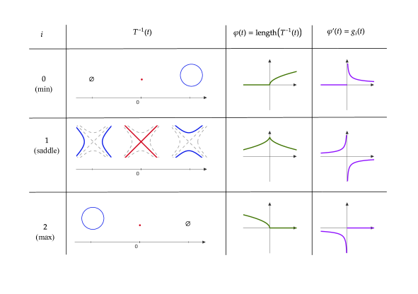
Figure 2. The picture illustrates the behavior of the length of level sets $T^{-1}(t)$ (assuming these are compact) of a Morse function $T\colon\mathbb{R}^{2}\to\mathbb{R}$, having only one critical point of index $i\in\{0,1,2\}$ with critical value $t=0$.

Proof.

we can assume that $t_{0}=0$ and look at what happens as $t\to 0^{+}$. The case $t\to 0^{-}$ can be deduced by considering the Morse function $-T$.

Let $h(x):=\frac{\tilde{\Delta}T(x)}{\|d_{x}T\|^{2}}$. Then, we have that $|\varphi^{\prime}(t)|=O(1)+|\int_{Z_{t}^{1}}hdZ_{t}^{1}|$. We can study the second term as in LABEL:eq:hSigmat.

Let us start from the easiest case: when $i=2$, it means that $0$ is a local maximum value for $T$,thus for $t>0$ we have $Z_{t}^{1}=\emptyset$, hence $g_{2}(t)=0$ for $t\geq 0$.

In the case $n_{-}=0$, we have that $0$ is a local minimum value for $T$. Let us denote $u=x_{+}=(u_{1},u_{2})$ Then, for all $t\in[0,\varepsilon]$, we have that $Z_{t}^{1}=x^{-1}(\sqrt{t}S^{1})$, thus $\varphi^{\prime}(t)=O(1)$

(6.36) $$\int_{Z_{t}^{1}}hdZ_{t}^{1} =t^{\frac{1}{2}}\int_{S^{1}}\mathcal{J}_{g}(dT(\sqrt{t}u)))h(\sqrt{t}u)dS^{1}(u).$$

$$=\frac{t^{-\frac{1}{2}}}{2}\int_{S^{1}}\mathcal{J}_{g}(dT(\sqrt{t}u)))\frac{1}{\alpha_{1}u_{1}^{2}+\alpha_{2}u_{2}^{2}}\left(\alpha_{1}+\alpha_{2}-\frac{\alpha_{1}^{2}u_{1}^{2}+\alpha_{2}^{2}u_{2}^{2}}{\alpha_{1}u_{1}^{2}+\alpha_{2}u_{2}^{2}}+o(1)\right)dS^{1}(u).$$

$$=\frac{t^{-\frac{1}{2}}}{2}\int_{S^{1}}\mathcal{J}_{g}(dT(\sqrt{t}u)))\frac{2\alpha_{1}\alpha_{2}}{\left(\alpha_{1}u_{1}^{2}+\alpha_{2}u_{2}^{2}\right)^{2}}dS^{1}(u)$$

$$=\Theta\left(\frac{1}{\sqrt{t}}\right)=\Theta\left(g_{0}(t)\right).$$

Now consider the more complicated case: when $n_{-}=n_{+}=i=1$. Define $\mu(u,v,r):=\left(\mathcal{J}_{g}(dT(\psi_{t}(u,v,r)))\right)$. Then, by LABEL:eq:hSigmat, we have that

(6.37) $$\int_{Z_{t}^{1}}hdZ_{t}^{1} =\sqrt{t}\sum_{(u,v)\in S^{0}\times S^{0}}\int_{0}^{\frac{\varepsilon}{\sqrt{t}}}h(\psi_{t}(u,v,s\sqrt{t}))\sqrt{2s^{2}+1}(s^{2}+1)^{-\frac{1}{2}}\mu(u,v,s\sqrt{t})ds.$$

Using the the coordinate $x=(x_{+},x_{-})$ discussed in Subsection 6.2.1, we have

(6.38) $$h(\psi_{t}(u,v,s\sqrt{t})) =\frac{\frac{1}{2t}}{(\alpha+\beta)s^{2}+\alpha}\left(\alpha-\beta+\frac{(\beta^{2}-\alpha^{2})s^{2}-\alpha^{2}}{(\alpha+\beta)s^{2}+\alpha}+o(1)\right)$$

$$=\frac{1}{2t}\left(\frac{-\alpha\beta}{\left[(\alpha+\beta)s^{2}+\alpha\right]^{2}}+\frac{o(1)}{(\alpha+\beta)s^{2}+\alpha}\right)$$

$$=\frac{-\frac{\beta}{\alpha}}{2t}\left(\frac{1}{\left[\nu^{2}s^{2}+1\right]^{2}}+\frac{o(1)}{\nu^{2}s^{2}+1}\right)$$

where $\nu=\sqrt{1+\frac{\beta}{\alpha}}$ depend only on $\mathrm{Hess}(T)_{0}$ and $g_{0}$. By construction, there are two positive constants $c_{1},c_{2}>0$ such that $\mu(u,v,r)\in[c_{1},c_{2}]$. For any parameter $\delta>0$ we can choose $\varepsilon=\varepsilon(\delta)$ so small that $|o(1)|\leq\delta$. Then, we will need to choose $\delta=\delta(\nu)$ small enough and, consequently, $\varepsilon=\varepsilon(\delta(\nu))$.

(6.39) $$\int_{Z_{t}^{1}}hdZ_{t}^{1} =\frac{-\frac{\beta}{\alpha}}{2\sqrt{t}}\sum_{(u,v)}\int_{0}^{\frac{\varepsilon}{\sqrt{t}}}\left(\frac{1}{\left[\nu^{2}s^{2}+1\right]^{2}}+\frac{o(1)}{\nu^{2}s^{2}+1}\right)\sqrt{\frac{2s^{2}+1}{(s^{2}+1)}}\mu(u,v,s\sqrt{t})ds\leq\dots$$

$$\dots\leq\frac{-C}{\sqrt{t}}\left(\left(\int_{0}^{+\infty}\frac{ds}{\left(\nu^{2}s^{2}+1\right)^{2}}\right)-\delta\left(\int_{0}^{+\infty}\frac{ds}{\nu^{2}s^{2}+1}\right)\right)c_{1}\leq\dots$$

$$\dots\leq-\frac{1}{\sqrt{t}}C^{\prime}=C^{\prime}g_{1}(t).$$

where the last inequality holds, for some positive constants $C,C^{\prime}>0$, as soon as we choose $\delta(\nu)$ small enough, since both integrals in the previous line are finite. A lower bound $\varphi^{\prime}(t)\geq-C^{\prime\prime}\frac{1}{\sqrt{t}}$ holds as well, by Theorem 6.5, thus we have proved that $\varphi^{\prime}(t)=\Theta(g_{1}(t))$, as $t\to 0^{+}$. ∎

Proposition 6.10.

Let $M={\kern 0.0ptM}^{\mathrm{o}}\sqcup\partial M$ be a compact Riemannian $\mathcal{C}^{2}$ surface with boundary and let $T\colon M\to\mathbb{R}$ be a Morse function. Assume that $t_{0}$ is a critical value of $T$ with critical set $C\subset{\kern 0.0ptM}^{\mathrm{o}}$. Then the function $\varphi^{\prime}(t):=\frac{d}{dt}\operatorname{\mathcal{H}}_{1}(\{T=t_{0}+t\})$ behaves as $\frac{1}{\sqrt{t}}$ on at least one side of $0$ unless there are at least three critical points $p_{0},p_{1},p_{2}\in C$ of Morse index $0,1,2$, respectively.

Proof.

The function $\varphi^{\prime}(t)$ behaves as the sum of the local behavior around each critical point $p\in C$. In other words, if we partition $C=C_{0}\sqcup C_{1}\sqcup C_{2}$ according to the Morse index, then we have

(6.40) $$\varphi^{\prime}(t)=O(1)+\Theta\left(\sum_{i=0,1,2}\#(C_{i})A_{i}g_{i}(t)\right),$$

as $t\to 0$. Where $A_{i}>0$ are some constants. then It is clear from Lemma 6.9 (see also Figure 2) that the only way in which the above sum could behave differently than $\frac{1}{\sqrt{|t|}}$ on both sides of $t=0$ is if $\#(C_{0})A_{0}=\#(C_{2})A_{2}=\#(C_{1})A_{1}$, which implies that $\#(C_{i})>0$ for all $i\in\{0,1,2\}$. ∎

6.3.1. Lower asymptotics for a two-dimensional manifold with boundary

Lemma 6.9 holds in a weaker form, when the manifold has boundary.

Proposition 6.11.

Let $t_{0}$ be a critical value of $T$ and assume that $p\in\partial M$ is the only critical point in $T^{-1}(t_{0})$, then $|\varphi^{\prime}(t)|=\Theta\left(\frac{1}{\sqrt{|t-t_{0}|}}\right)$ for $t\to t_{0}^{+}$, or for $t\to t_{0}^{-}$.

Proof.

We have by Equation 6.31 and the discussion thereafter, we have

(6.41) $$\varphi^{\prime}(t_{0}+t)=-\sum_{p\in\partial Z_{t}}\frac{g(\mathbf{n},\nu)|_{p}}{\|d_{p}(T|_{\partial M})\|}+O(1),$$

Assume that $p$ is a minimum of $T|_{\partial M}$. Then, there is a $\mathcal{C}^{1}$ coordinate chart $\varphi\colon U\to\mathbb{R}^{2}$ around $p=\varphi^{-1}(0,0)$ such that

(6.42) $$\varphi(U)=\left\{(x,y)\colon x\in(-1,1),\ \varepsilon y\geq\varepsilon x^{2}\right\},\quad\text{and}\quad T\circ\varphi^{-1}(x,y)=y,$$

where $\varepsilon=-\mathrm{sign}(g(\mathbf{n},\nu)|_{p})\in\{-1,1\}$ (see [24, Lemma de Morse $\mathcal{C}^{r}$ à paramètres]). For simplicity, assume that $W=U$. Define $p_{\pm}(t)=(\pm\sqrt{t},t)$, then we have $\partial Z_{t}=\{p_{-}(t),p_{+}(t)\}$ and $T_{p_{\pm}(t)}\partial M=\mathrm{span}\{\partial_{x}\pm 2\sqrt{t}\partial_{y}\}$.

(6.43) $$\|d_{p}(T|_{\partial M})\|=\left|g\left(\mathrm{grad}f,\frac{\partial_{x}\pm 2\sqrt{t}\partial_{y}}{\|\partial_{x}\pm 2\sqrt{t}\partial_{y}\|}\right)\right|=\frac{2\sqrt{t}}{\|\partial_{x}\pm 2\sqrt{t}\partial_{y}\|}.$$

We conclude that $|\varphi^{\prime}(c+t)|\geq\frac{C}{\sqrt{t}}$ for some $C>0$. ∎

Remark 6.12.

In the boundary case, one can formulate a suitable generalization of Proposition 6.10. However, in this case the situation is less rigid, indeed the local behavior around each critical point at the boundary can take all the four forms: $\pm g_{0}(t),\pm g_{2}(t)$, depending on the index $i$ as a critical point of $T|_{\partial M}$ ($i=0$ if the point is a local minimum and $i=1$ if it is a local maximum) and on the sign $s_{\mathbf{n}}$ of $dT(\mathbf{n})$ at the critical point, where $\mathbf{n}$ is the outer normal vector to the boundary. If we denote as $s_{\partial}$ the sign of $2i-1$, then we have:

(6.44) $$\varphi^{\prime}(t)=O(1)+\Theta\left(s_{\mathbf{n}}s_{\partial}\cdot g_{2i}(t)\right)$$

(see Figure 3 and Figure 4).

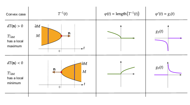
Figure 3. The picture illustrates the behavior of the length of level sets $T^{-1}(t)$ of a Morse function $T\colon M\to\mathbb{R}$, where $M$ is a compact domain in $\mathbb{R}^{2}$ and $T$ is the projection on the horizontal axis, $T(x,y)=x$. There are four qualitatively different cases in total, depending on the convexity of the domain near the critical point. Two are depicted above and the other two are in Figure 4.

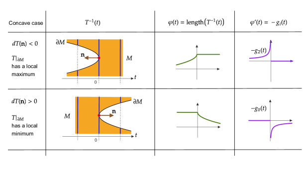
Figure 4. See the caption of Figure 3.

7. The nodal volume along transverse curves

In this section we put together the results of Section 5 and of Section 6 in order to complete our study of the function $\varphi(t)=V(f_{t})$, where $(f_{t})_{t\in I}$ is a transverse curve in $\mathcal{C}^{2}(M)$, see Theorem 7.1 and Definition 7.3 below. Taking up the discussion started at the beginning of Section 5, this study is aimed at giving criteria for verifying the condition of ray-absolute continuity, (i) of Definition 3.6, that is an important part of the proof of Theorem 1.2. Indeed, Theorem 7.1 and Corollary 7.5 below essentially characterize the Sobolev regularity of the restriction of the nodal volume functional $V$ to random segments $[X,X+h]$ in $\mathcal{C}^{2}(M)$, given that, by Theorem 5.10, such segments are transverse curves with probability one.

Furthermore, the continuity part of Theorem 7.1, stating that $\varphi$ is continuous, combined in particular with the results of Section 3, allows us to prove point (i) of Theorem 1.2, with the exception of the description of the singular part of the law (Equation 1.1), which will be discussed in Section 10. Theorem 7.6 states the existence of an absolutely continuous component of the law of $V(X)$ and Proposition 7.7 ensures that its support is an interval.

7.1. Sobolev regularity of the nodal volume

The following deterministic result is one of the key point of the paper. Observe that Equation 7.1 provides an intuitive justification of the results (ii),(iii) and (iv) of Theorem 1.2. Indeed, it is an important ingredient of the proofs of Theorem 9.2, Theorem 9.5 and Theorem 9.7.

Theorem 7.1.

Let Assumption A prevail. Let $I$ be a bounded interval, let $(f_{t})_{t\in I}$ be a $\mathcal{C}^{2}$ transverse curve in $\mathcal{C}^{2}(M)$, then $I_{c}=\left\{t\in I\colon f_{t}\notin\mathcal{U}\right\}$ is finite. Define $\varphi(t)=V(f_{t})$ then $\varphi\in\mathcal{C}^{0}(I)\cap\mathcal{C}^{1}(I\smallsetminus I_{c})$. There is a constant $C>0$ such that for any $t_{0}\in I_{c}$,

(7.1) $$|\varphi^{\prime}(t_{0}+t)|\leq C\left\{\begin{aligned} &1,\quad\text{if }m\geq 4\\ &|\log t|,\quad\text{if }m=3;\\ &t^{-\frac{1}{2}},\quad\text{if }m=2.\end{aligned}\right.$$

In particular, $\varphi\in W^{1,1}(I)$; if $m\geq 3$, then $\varphi\in W^{1,k}(I)$ for all $k\in\mathbb{N}$. Moreover, if $m\geq 4$, then $\varphi\in\mathcal{C}^{1}(I)$.

Proof.

By Corollary 5.11, there exists a $\mathcal{C}^{2}$ Riemannian manifold with boundary $N$ and a Morse function $T\colon N\to\mathbb{R}$ such that $\varphi(t)=\operatorname{\mathcal{H}}^{m-1}(T^{-1}(t))$, so the statement follows from Lemma 6.6. ∎

Remark 7.2.

One might be led to think that $\varphi\in\mathcal{C}^{0}(I)\cap\mathcal{C}^{1}(I\smallsetminus I_{c})$, with $I_{c}$ finite, is enough to conclude that $\varphi$ is absolutely continuous. Indeed, $t_{0},t_{1}\in I_{0}$, the following limit exists:

(7.2) $$\varphi(t_{1})-\varphi(t_{0})=\lim_{\varepsilon_{0},\varepsilon_{1}\to 0^{+}}\varphi(t_{1}-\varepsilon_{1})-\varphi(t_{0}+\varepsilon_{0})=\lim_{\varepsilon_{1},\varepsilon_{2}\to 0^{+}}\int_{t_{0}+\varepsilon_{0}}^{t_{1}-\varepsilon_{1}}\varphi^{\prime}.$$

The existence of the rightmost limit, does not imply that the function $\varphi^{\prime}$ is integrable in the considered interval, i.e., that $\varphi^{\prime}\in L^{1}([t_{0},t_{1}])$. A counterexample is the function $\varphi(x)=\frac{1}{x}\sin\left(\frac{1}{x}\right)$.

7.2. Sobolev (non)regularity in dimension $2$

Definition 7.3.

Let $f_{0},e\in E$ and let $\ell=f_{0}+\mathbb{R}e$. We say that $\ell$ is a non-compensating transverse line if $\ell\mathrel{\text{\raise-0.43057pt\vbox{ \halign{#\cr\smash{$-$}\crcr$\pitchfork$\crcr} }}}\mathcal{W}$ (in the sense of Definition 5.7) and if, whenever $f=f_{0}+t_{0}e\in\mathcal{W}$, we have that:

1. $0$ is a (strat.) Morse critical value of $f$ ;

2. $\text{CZ}_{f}\subset{\kern 0.0ptM}^{\mathrm{o}}$, or $\text{CZ}_{f}=\{p\}$ is one point;

3. the symmetric forms $e(p)\mathrm{Hess}_{p}f$ all have the same index for every $p\in C$.

From Theorem 5.12 we can deduce the following results concerning a Gaussian field $X\mathchoice{\raisebox{-1.50696pt}{$\displaystyle{{}^{\subset}}$}\mkern-11.5mu\raisebox{1.93747pt}{$\displaystyle{{}_{\subset}}$}}{\mkern 1.0mu\raisebox{-1.1625pt}{$\textstyle{{}^{\subset}}$}\mkern-11.7mu\raisebox{1.93747pt}{$\textstyle{{}_{\subset}}$}}{\raisebox{1.50696pt}{$\scriptstyle\subset$}\mkern-14.0mu\raisebox{-0.6458pt}{$\scriptstyle\subset$}}{\raisebox{1.29167pt}{$\scriptscriptstyle\subset$}\mkern-13.5mu\raisebox{-0.43057pt}{$\scriptscriptstyle\subset$}}\mathcal{C}^{2}(M)$.

Corollary 7.4.

Let Assumption A prevail. Assume that there are no pairs of points $p,q\in\partial M$ such that the random vectors $j^{1}_{p}X|_{\partial M},j^{1}_{q}X|_{\partial M}$ in $J^{1}(\partial M,\mathbb{R})$ are completely correlated. Then, for every $e\neq 0\in E$, almost surely, $X+\mathbb{R}e$ is a non-compensating transverse line.

Proof.

This is a direct consequence of Theorem 5.12. Theorem 5.12 immediately implies condition (1) of Definition 7.3. Point (3) of Theorem 5.12 implies that $CZ_{f}\subset{\kern 0.0ptM}^{\mathrm{o}}$ or $CZ_{f}\subset\partial M$. Moreover, Condition (5) of Theorem 5.12 is satisfied by a pair of points $p,q\in\partial M$ only if $p=q$, thus we deduce property (2) of Definition 7.3. Finally, condition (4) of Definition 7.3 corresponds to point (3) of Theorem 5.12. ∎

Corollary 7.5.

Let Assumption A prevail with $\dim M=2$. Assume that there are no pairs of points $p,q\in\partial M$ such that the random vectors $j^{1}_{p}X|_{\partial M},j^{1}_{q}X|_{\partial M}$ in $J^{1}(\partial M,\mathbb{R})$ are completely correlated. Then, for every $e\neq 0\in E$, almost surely, either $X+\mathbb{R}e\subset\mathcal{U}$, or the function $t\mapsto V(X+te)$ is not in the space $W^{1,2}(\mathbb{R})$.

Proof.

Let $\varphi(t)=V(X+te)$. Corollary 7.4 implies that $X+\mathbb{R}e$ is a non-compensating transverse line. From Proposition 6.10, since there cannot be three critical points of different index, we know that if $\text{CZ}\subset{\kern 0.0ptM}^{\mathrm{o}}$, then $(\varphi^{\prime})^{2}$ is not integrable in a neighborhood of a critical value $t_{0}$. If $\text{CZ}=\{p\}\subset\partial M$, the same is true, as it follows from Proposition 6.11. It follows that the only situation in which $(\varphi^{\prime})^{2}$ is integrable is if there are no points $t\in\mathbb{R}$ such that $f+te\notin\mathcal{U}$. ∎

7.3. Absolute continuity of the nodal volume

Let us consider the setting of Section 3, with $\mu$ being the Gaussian measure induced by $X$ on its topological support $E\subset\mathcal{C}^{2}(M)$ and $V\colon E\to\mathbb{R}$ being the restriction of the nodal volume functional.

Theorem 7.6.

Let Assumption A prevail. If $V(X)$ is non-constant, then the law of $V(X)\mathchoice{\raisebox{-1.50696pt}{$\displaystyle{{}^{\subset}}$}\mkern-11.5mu\raisebox{1.93747pt}{$\displaystyle{{}_{\subset}}$}}{\mkern 1.0mu\raisebox{-1.1625pt}{$\textstyle{{}^{\subset}}$}\mkern-11.7mu\raisebox{1.93747pt}{$\textstyle{{}_{\subset}}$}}{\raisebox{1.50696pt}{$\scriptstyle\subset$}\mkern-14.0mu\raisebox{-0.6458pt}{$\scriptstyle\subset$}}{\raisebox{1.29167pt}{$\scriptscriptstyle\subset$}\mkern-13.5mu\raisebox{-0.43057pt}{$\scriptscriptstyle\subset$}}\mathbb{R}$ and the Lebesgue measure are not mutually singular.

Proof.

We want to apply Corollary 3.4. To do so, considering Lemma 5.2 and Theorem 4.6, we only need to show that there is a connected component of $\mathcal{U}\cap E\subset E$ on which $V$ is not a constant function. By contradiction, if $V$ were constant on each connected component of $\mathcal{U}\cap E$, then $V(\mathcal{U}\cap E)$ should be countable, since $E$ is a II-countable space. By Theorem 5.10, for any two connected components of $\mathcal{U}\cap E$, there is a transverse curve in $E$ connecting one to the other. This means that any two points $f_{0},f_{1}\in\mathcal{U}\cap E$ are connected by a transverse curve $c:[0,1]\to E$, so that $c^{-1}(E\smallsetminus\mathcal{U})$ is a finite, or empty, subset $I_{c}\subset[0,1]$. Now, Theorem 7.1 ensures that $\varphi=V\circ c$ is continuous, hence $[V(f_{0}),V(f_{1})]\subset\varphi([0,1])=V(\mathcal{U}\cap E)\cup V(I_{c})$ is countable, which implies that $V(f_{1})=V(f_{2})$. Applying the latter argument to every pair $f_{1},f_{2}\in\mathcal{U}\cap E$, we conclude that $V$ is constant on $\mathcal{U}\cap E$, which contradicts the hypothesis. ∎

Proposition 7.7.

Let Assumption A prevail. The topological support of the random variable $V(X)$ is the set $\overline{V(\mathcal{U}\cap E)}$ and it is an interval. Moreover, $\overline{V(\mathcal{U}\cap E)}\smallsetminus V(\mathcal{U}\cap E)$ is locally finite.

Proof.

Let $S\subset\mathbb{R}$ be the topological support of $V(X)$, that is, the smallest closed set of probability one. $V(\mathcal{U}\cap E)\subset\mathbb{R}$ is an event of probability one for $V(X)$, thus $S\subset\overline{V(\mathcal{U}\cap E)}$. On the other hand, since $V$ is continuous on the open set $\mathcal{U}$, the set $V^{-1}(\mathbb{R}\smallsetminus S)\cap\mathcal{U}\cap E$ is open in $E$. Clearly, it has probability zero, so it must be empty. From this, we deduce that $V(\mathcal{U}\cap E)\subset S$ which implies that $S=\overline{V(\mathcal{U}\cap E)}$.

Now we prove that $\overline{V(\mathcal{U}\cap E)}$ is an interval. For any two connected components of $\mathcal{U}\cap E$, there is a transverse curve connecting one to the other. This implies that any two points in $\mathcal{U}\cap E$ are connected by a transverse curve. Theorem 5.10 shows that a transverse curve is always contained in $\mathcal{U}\sqcup\mathcal{U}^{\prime}\cap E$ and any point in $\mathcal{U}\sqcup\mathcal{U}^{\prime}\cap E$ lies on some transverse curve, by Corollary 5.9; moreover, Theorem 7.1 states that $V$ is continuous along a transverse curve. From this, we can conclude that the set $V(\mathcal{U}\sqcup\mathcal{U}^{\prime}\cap E)$ is an interval and that $V(\mathcal{U}\sqcup\mathcal{U}^{\prime}\cap E)\subset\overline{V(\mathcal{U}\cap E)}$. It follows that $\overline{V(\mathcal{U}\sqcup\mathcal{U}^{\prime}\cap E)}=\overline{V(\mathcal{U}\cap E)}$ is also an interval. Moreover, since a transverse curve is contained in $\mathcal{U}$ for all but a locally finite set of times, we conclude that $\overline{V(\mathcal{U}\sqcup\mathcal{U}^{\prime}\cap E)}\smallsetminus V(\mathcal{U}^{\prime}\cap E)$ is locally finite. ∎

Remark 7.8.

In the above proofs, we used only the results discussed up to Subsection 5.3, with the exception of Theorem 7.1. However, we don’t need the full power of the latter: the only thing that is needed is Lemma 6.6, ensuring the continuity of the nodal volume of the level sets of a Morse function. This is a quite direct consequence of Morse Lemma 6.1. In particular, in the proof of Lemma 6.6, we deduced it from a very simple sub-case ($k=0$, and $h=1$) of Theorem 6.5. Considering that, we can say that Theorem 7.6 and Proposition 7.7 rely only on the results discussed up to Subsection 5.3 and on Morse Lemma.

8. Preliminary lemmas

This section is devoted to a study of the integrability of $\|d_{X}V\|_{\mathcal{H}_{X}}^{2}$, with the purpose of checking the validity of condition (iii) of Definition 3.6, for the nodal volume random variable $V(X)$.

Let $X\mathchoice{\raisebox{-1.50696pt}{$\displaystyle{{}^{\subset}}$}\mkern-11.5mu\raisebox{1.93747pt}{$\displaystyle{{}_{\subset}}$}}{\mkern 1.0mu\raisebox{-1.1625pt}{$\textstyle{{}^{\subset}}$}\mkern-11.7mu\raisebox{1.93747pt}{$\textstyle{{}_{\subset}}$}}{\raisebox{1.50696pt}{$\scriptstyle\subset$}\mkern-14.0mu\raisebox{-0.6458pt}{$\scriptstyle\subset$}}{\raisebox{1.29167pt}{$\scriptscriptstyle\subset$}\mkern-13.5mu\raisebox{-0.43057pt}{$\scriptscriptstyle\subset$}}\mathcal{C}^{2}(M)$ be a Gaussian satifying Assumption A. Let $C(p,q)=\mathbb{E}\left\{X(p)X(q)\right\}$ be its covariance function. Then, $C\colon M\times M\to\mathbb{R}$ is semipositive definite, symmetric and of class $\mathcal{C}^{2,2}(M\times M)$.

8.1. Kac-Rice formula on the zero set

8.1.1. Degenerations are few

Define

(8.1) $$\Delta^{X}:=\left\{(p,q)\in M^{2}:(X(p),X(q))\text{ is degenerate}\right\}$$

The diagonal $\Delta:=\left\{(p,p)\colon p\in M\right\}\subset M\times M$ is, in general, a subset of $\Delta^{X}$. Notice that $\Delta^{X}$ is closed.

Lemma 8.1.

For every $p\in M,$ the set $M_{p}^{X}=\Delta^{X}\cap(\{p\}\times M)$ is finite. Moreover, there is a neighborhood $B(\Delta)$ of the true diagonal in $M\times M$ such that $B(\Delta)\cap\Delta^{X}=\Delta$.

Proof.

It is equivalent to prove the statement for the normalized field $\mathbb{E}\{|X|\}^{-1}X$, so we may assume that $\mathbb{E}|X(p)|^{2}=1$ for all $p$. In this case, we have

(8.2) $$M_{p}^{X}=\left\{q\in M:X(p)=\pm X(q)\text{ a.s.}\right\}.$$

Let $C$ be the covariance function of $X$ and let $h_{p}:=C(p,\cdot).$ Then $M_{p}^{X}=h_{p}^{-1}(\left\{-1,1\right\}),$ moreover $|h_{p}(q)|\leq 1$ for all $q\in M,$ by Cauchy-Schwartz, so it is sufficient to show that $h_{p}$ has non-degenerate second derivative at the points $q\in M_{p}^{X}.$ This follows from:

(8.3) $$d^{2}_{q}h_{p}=\mathbb{E}\{X(p)d^{2}_{q}X\}=\mathbb{E}\{X(q)d^{2}_{q}X\}=-\mathbb{E}\{d_{q}X(d_{q}X)^{T}\}.$$

We prove the last part by contradiction: we assume that the conclusion is false, that is, we assume that there exists a sequence $(p_{n},q_{n})\in\Delta^{X}\smallsetminus\Delta$ converging to a point $(p,p)$ in the true diagonal. Notice that this means that $X(p_{n})=X(q_{n})$ almost surely. Then, passing to a subsequence we can assume that in a local chart around $p$ we have

(8.4) $$\frac{p_{n}-q_{n}}{|p_{n}-q_{n}|}\to v\in T_{p}M\smallsetminus\{0\}.\quad\text{ hence }\quad 0=\frac{X(p_{n})-X(q_{n})}{|p_{n}-q_{n}|}\xrightarrow{a.s.}d_{p}X(v).$$

This contradicts the nondegeneracy of $j^{1}_{p}X$, so we conclude that such a sequence does not exist. ∎

8.1.2. The double field is z-KROK

Taking up the language of [66], a random field is said to be z-KROK if, roughly speaking, the Kac-Rice formula (see [9, 2]) for its zero set behaves well. Such concept is analogous to the hypotheses of [9, Theorem 6.10]

Lemma 8.2.

The mapping $(p,q)\mapsto(X(p),X(q))$ defines a $\mathcal{C}^{2}$ Gaussian random map $X^{\times 2}\colon M\times M\to\mathbb{R}^{2}$ for which $(0,0)$ is a regular value almost surely. Moreover, its restriction to $M\times M\smallsetminus\Delta^{X}$ is z-KROK in the sense of [66] and we have the following formula: let $Z=X^{-1}(0)$ and $\alpha\colon\mathcal{C}^{1}(M)\times M\times M\to\mathbb{R}$ be a Borel function, then

(8.5) $$\mathbb{E} \left\{\int_{Z}\int_{Z}\alpha(X,p,q)dZ(p)dZ(q)\right\}=\dots$$

$$\dots&=\int_{M\times M\smallsetminus\Delta^{X}}\mathbb{E}\left\{\alpha(X,p,q)\|d_{p}X\|\|d_{q}X\|\Bigg{|}\begin{aligned} X(p)&=0\\ X(q)&=0\end{aligned}\right\}\frac{dM(p)dM(q)}{2\pi\sqrt{C(p,p)C(q,q)-C(p,q)^{2}}}.$$

Proof.

First, observe that since the Gaussian field $X$ satisfies the hypotheses of Bulynskaya Lemma 5.2, thus, with probability one, $0$ is regular value of $X$ and $Z\subset M$ is a $\mathcal{C}^{2}$ hypersurface. This implies that $(0,0)$ is almost surely a regular value for the map $X^{\times 2},$ as well. Moreover, for any $(p,q)\in U^{X}:=M\times M\smallsetminus\Delta^{X}$ we have that $X^{\times 2}(p,q)$ has a density in $\mathbb{R}^{2}$. From this, we see that random function $X^{\times 2}|_{U^{X}}$ satisfies the hypotheses of [66, Prop. 4.9], thus it is a z-KROK random field.

Observe that if $m\geq 2,$ then $Z\times Z\cap\Delta^{X}$ has zero $2(m-1)$-volume, because of Lemma 8.1, so that the left-hand-side of Equation 8.5 can be seen as an integral over the set $\{X^{\times 2}=(0,0)\}.$ Therefore, by [66, Thm. 6.2] we obtain the wanted formula. ∎

Note that if $\alpha$ is defined only on the subset $\mathcal{Z}=\{(f,p,q)\in\mathcal{C}^{2}(M)\times M\times M:f\mathrel{\text{\raise-0.43057pt\vbox{ \halign{#\cr\smash{$-$}\crcr$\pitchfork$\crcr} }}}0,f(p)=f(q)=0\},$ then the formula still holds. To see this, observe that $\mathcal{Z}$ is a Borel subset, so $\alpha$ can be extended to a global Borel $\alpha^{\prime}$ function, for which we can apply the theorem. In the end, however, the formula depends only on the restriction $\alpha^{\prime}|_{\mathcal{Z}}=\alpha.$

8.2. Uniform integrability of rational functions of Gaussian vectors

In this subsection we will consider the space $\mathcal{X}$ of Gaussian vectors in $\mathbb{R}^{N_{0}}\times\mathbb{R}^{N_{1}}\times\mathbb{R}^{N_{2}}$. Elements of this space are random vectors $X=(X_{0},X_{1},X_{2})\sim N(0,K)$, identified by their covariance matrix:

(8.6) $$K=\begin{pmatrix}K_{00}&K_{01}&K_{02}\\ {}&K_{11}&K_{12}\\ {}&{}&K_{22}\end{pmatrix}.$$

Hence, $\mathcal{X}$ can be identified with the space of symmetric semi-positive definite matrices $K$ of size $N=N_{0}+N_{1}+N_{2}$. For $A,B\in\mathbb{N}$, let $\mathcal{X}_{A,B}\subset\mathcal{X}$ be the open subset such that $\mathrm{rank}(K_{11})\geq A$ and $\mathrm{rank}(K_{22})\geq B.$

Remark 8.3.

For any $A\in\mathbb{N}$ the condition $\mathrm{rank}(K_{11})\geq A$ is equivalent to have that

(8.7) $$\mathbb{E}\left\{\frac{1}{\|X_{1}\|^{A-1}}\right\}<\infty.$$

At the same time we will consider the space of sub-polynomial functions $\mathcal{F}$. An element $F\in\mathcal{F}$ is a measurable function $F\colon\mathbb{R}^{N}\to\mathbb{R}$ such that there exists a constant $D>0$ such that

(8.8) $$|F(x)|\leq D(1+|x|^{D}),\text{ for all $x\in\mathbb{R}^{N}.$}$$

We will call $\mathcal{F}_{D}$ the subset of $\mathcal{F}$ on which (8.8) holds with the constant $D$. We put on $\mathcal{F}_{D}$ the topology of point-wise convergence.

We need some criteria for the convergence of integrals of the form

(8.9) $$I_{a,b}(F,K)=\mathbb{E}F(X)\|X_{1}\|^{-a}\|X_{2}\|^{-b},$$

with $a,b\in\mathbb{N}.$

A first idea is that $I_{a,0}$ should be continuous on $\mathcal{F}_{D}\times\mathcal{X}_{A,0}$ if $a<A$. Indeed, when $\|X_{1}\|=\chi_{A}$ is a chi random variable of parameter $A$, we have that $\mathbb{E}\{\chi_{A}^{-a}\}<\infty$ if and only if $a<A.$

A second idea is that $I_{a,b}$ should be continuous on $\mathcal{F}_{D}\times\mathcal{X}_{A,B}$ if $2a<A$ and $2b<B$. Indeed, by Cauchy-Schwartz, we have that $\mathbb{E}\{\chi_{A}^{-a}\chi_{B}^{-b}\}^{2}<\mathbb{E}\{\chi_{A}^{-2a}\}\mathbb{E}\{\chi_{B}^{-2b}\}.$

A third idea (which may be overkill) is that $I_{a,b}$ should be continuous on $\mathcal{F}_{D}\times\mathcal{X}_{A,B}$ if $pa<A$ and $qb<B$ for some conjugated exponents $p$ and $q$, that is, $\frac{1}{p}+\frac{1}{q}=1.$ Indeed, by Holder inequality, we have that $\mathbb{E}\{\chi_{A}^{-a}\chi_{B}^{-b}\}<\mathbb{E}\{\chi_{A}^{-pa}\}^{\frac{1}{p}}\mathbb{E}\{\chi_{B}^{-qb}\}^{\frac{1}{q}}.$ The case $b=0$ can be interpreted with $p=1$ and $q=+\infty.$

Theorem 8.4.

$I_{a,b}$ is continuous on $\mathcal{F}_{D}\times\mathcal{X}_{A,B}$ if $pa<A$ and $qb<B$ for some conjugated exponents $p$ and $q$, that is, $\frac{1}{p}+\frac{1}{q}=1.$ Moreover, for all $(F,K)\in\mathcal{F}_{D}\times\mathcal{X}_{N_{1},N_{2}}$ such that $\|K\|\leq D$, we have

(8.10) $$I_{a,b}(F,K)\leq C(D)\left(1+\frac{1}{\sqrt{\det K_{11}}}+\frac{1}{\sqrt{\det K_{22}}}\right)$$

Corollary 8.5.

$I_{1,1}$ is continuous on $\mathcal{F}_{D}\times\mathcal{X}_{3,3}$.

Proof.

Set $p=q=2$, then $p\cdot 1=2<3.$ ∎

Proof of Theorem 8.4.

Let $K(n)\to K$ in $\mathcal{X}_{A,B}$, as $n\to+\infty$. Let $X(n)\to X$ be the corresponding sequence of Gaussian vectors, which we can assume to be almost surely convergent. Let $L(n)\to L$ be a converging sequence of matrices such that $L(n)L(n)^{T}=K(n)$. Then

(8.11) $$I_{a,b}(F_{n},K_{n})=\frac{F_{n}(X(n)\gamma)}{|X_{1}(n)|^{a}|X_{2}(n)|^{b}}$$

To conclude, we will use Fatou Lemma in the form of the following argument. Young’s inequality $xy\leq\frac{a^{p}}{p}+\frac{y^{q}}{q}$ yields $|f_{n}|\leq g_{n},$ where:

(8.12) $$f_{n}:=\frac{F_{n}(X(n))}{|X_{1}(n)|^{a}|X_{2}(n)|^{b}}\quad g_{n}:=|F_{n}(X(n))|\left(\frac{1}{p|X_{1}(n)|^{ap}}+\frac{1}{q|X_{2}(n)|^{bq}}\right).$$

We have that $f_{n}\to f=\frac{F(X)}{|X_{1}|^{a}|X_{2}|^{b}}$ and $g_{n}\to g=|F(X)|\left(\frac{1}{p|X_{1}|^{ap}}+\frac{1}{q|X_{2}|^{bq}}\right)\geq|f|$ a.s. Thus, in order to prove that $\mathbb{E}f_{n}\to\mathbb{E}f$, it is sufficient to show that $\mathbb{E}\left\{g_{n}\right\}<+\infty$ uniformly. We can reorder the variables and change the numbers $N_{0},N_{1},N_{2}$ to have $N_{1}=A,$ $N_{2}=B$, using the inequality $\frac{1}{\|x+y\|}\leq\frac{1}{\|x\|}$. Let $B_{A}\subset\mathbb{R}^{A}$ be the unit ball. Observe that

(8.13) $$\mathbb{E}\left\{\frac{|F_{n}(X(n))|}{|X_{1}(n)|^{ap}}\right\} \leq 2D\mathbb{E}\left\{\frac{1_{B_{A}}(X_{1}(n)}{|X_{1}(n)|^{ap}}\right\}+\mathbb{E}\left\{D(1+\|X_{1}(n)\|^{D})\right\}$$

$$\leq\frac{2D}{(2\pi)^{\frac{A}{2}}}\int_{B^{A}}\frac{1}{|x|}\frac{dx}{\sqrt{\det K_{11}(n)}}+\mathbb{E}\left\{D(1+(k\|\gamma_{1}\|)^{D})\right\},$$

where $k=\sup_{n}\|K(n)\|<\infty$ and $\gamma_{1}$ is a standard Gaussian vector in $\mathbb{R}^{A}$. Thus, for some constant $C$, we have an inequality

(8.14) $$\mathbb{E}\left\{\frac{|F_{n}(X(n))|}{|X_{1}(n)|^{ap}}\right\}\leq\frac{C}{\sqrt{\det K_{11}(n)}}\int_{B^{A}}\frac{1}{|x|^{ap}}dx+C.$$

If the limit $K\in\chi_{A,B}$, then $\det K_{11}\neq 0$ and the integral is finite because $A>ap$. Repeating the same for the other term in $g_{n}$, we conclude. ∎

8.3. The conditional expectation is bounded

8.3.1. Differentiation of the conditioning

Lemma 8.6.

Let $(p_{n},q_{n})\in M\times M\smallsetminus\Delta$ be a sequence converging to a double point $(p,p)$. Assume that in some coordinate chart around $p$, we have

(8.15) $$\lim_{n\to\infty}\frac{p_{n}-q_{n}}{|p_{n}-q_{n}|}=v\in T_{p}M$$

Let $H_{n}\to Y$ be a converging sequence of Gaussian vectors in $\mathbb{R}^{k}$ such that $(H_{n},X(p_{n}),X(q_{n}))$ are jointly Gaussian. Then, we have the following convergence in law

(8.16) $$\left[H_{n}\ \Big{|}X(p_{n})=X(q_{n})=0\right]\implies\left[H\ \Big{|}X(p)=d_{p}X(v)=0\right].$$

Remark 8.7.

The above statement means that for any $\alpha\colon\mathbb{R}^{N}\to\mathbb{R}$ continuous and bounded, we have

(8.17) $$\lim_{t\to 0}\mathbb{E}\{\alpha(H_{n})|X(p_{n})=X(q_{n})=0\}=\mathbb{E}\{\alpha(H)|X(p)=d_{p}X(v)=0\}.$$

Proof.

Consider the family of non-degenerate Gaussian vectors $Y_{n}\mathchoice{\raisebox{-1.50696pt}{$\displaystyle{{}^{\subset}}$}\mkern-11.5mu\raisebox{1.93747pt}{$\displaystyle{{}_{\subset}}$}}{\mkern 1.0mu\raisebox{-1.1625pt}{$\textstyle{{}^{\subset}}$}\mkern-11.7mu\raisebox{1.93747pt}{$\textstyle{{}_{\subset}}$}}{\raisebox{1.50696pt}{$\scriptstyle\subset$}\mkern-14.0mu\raisebox{-0.6458pt}{$\scriptstyle\subset$}}{\raisebox{1.29167pt}{$\scriptscriptstyle\subset$}\mkern-13.5mu\raisebox{-0.43057pt}{$\scriptscriptstyle\subset$}}\mathbb{R}^{2}$ such that

(8.18) $$Y_{n}:=\left(X(p_{n}),\left(X(q_{n})-X(p_{n})\right)\frac{1}{|q_{n}-p_{n}|}\right)\xrightarrow[n\to\infty]{a.s.}Y:=\left(X(p),d_{p}X(v)\right)$$

Notice that in particular the inverse of the covariance matrix $K_{n}^{-1}=\mathbb{E}Y_{n}Y_{n}^{-T}$ is a convergent. Moreover, the sequence of matrices defined as $C_{n}:=\mathbb{E}\left\{H_{n}Y_{n}^{T}\right\}$ converges to the matrix $C=\mathbb{E}\left\{HY^{T}\right\}$.

Interpreting the conditioning as a projection, we can observe that for all $n\neq 0$, we have $[H_{n}|X(p_{n})=X(q_{n})=0]=[H_{n}|Y_{n}=0]$, because the $Y_{n}=0$ if and only if $X_{n}=X_{n}=0$. Furthermore, using Gaussian regression formula, we can write explicitely the sequence of conditioned Gaussian vectors (defined up to equivalence of their law, i.e., their covariance matrices) as follows

(8.19) $$\left(H_{n}\ \Big{|}X(p_{n})=X(q_{n})=0\right)=H_{n}-C_{n}K_{n}^{-1}Y_{n}\xrightarrow[n\to\infty]{a.s.}H-CK^{-1}Y.$$

The above almost sure convergence implies the convergence in law, which is what we wanted to show. ∎

8.3.2. The conditional expectation is bounded

Lemma 8.8.

Assume $\dim M\geq 4$. There is a constant $E>0$ and a neighborhood $B\supset\Delta$ of the diagonal, such that for all $(p,q)\in B\smallsetminus\Delta$, we have

(8.20) $$I(p,q)=\mathbb{E}\left\{\frac{|\tilde{\Delta}X(p)|}{\|d_{p}X\|}\frac{|\tilde{\Delta}X(q)|}{\|d_{q}X\|}\Bigg{|}\begin{aligned} X(p)&=0\\ X(q)&=0\end{aligned}\right\}\leq E.$$

Proof.

We will reduce the proof to the convergence of integrals treated in Corollary 8.5. Indeed $I(p,q)$ is an integral of the form $I_{1,1}(F_{p,q},K_{p,q}),$ where $K_{p,q}$ is the covariance function of the conditioned Gaussian vector $X_{p,q}=(X_{0},X_{1},X_{2}),$ defined as

(8.21) $$X_{p,q}=\begin{pmatrix}X_{0}\\ X_{1}\\ X_{2}\end{pmatrix}=\left[\begin{pmatrix}(\mathrm{Hess}_{p}X,\mathrm{Hess}_{q}X)\\ d_{p}X\\ d_{q}X\end{pmatrix}\Bigg{|}\begin{aligned} X(p)&=0\\ X(q)&=0\end{aligned}\right]=\left[Y(X,p,q)\Bigg{|}\begin{aligned} X(p)&=0\\ X(q)&=0\end{aligned}\right]$$

The function $F_{p,q}$ satisfies the inequality:

(8.22) $$F_{p,q}((H_{1},H_{2}),u,v) =|\left(\mathrm{tr}(g_{p}^{-1}H_{1})-\frac{1}{u^{T}g_{p}^{-1}u}u^{T}H_{1}u\right)\cdot\left(\mathrm{tr}(g_{q}^{-1}H_{2})-\frac{1}{v^{T}g_{q}^{-1}v}v^{T}H_{2}v\right)|$$

$$\leq D|H_{1}|\cdot|H_{2}|$$

for some $D>2$, hence $F_{p,q}\in\mathcal{F}_{D}$ for all $p,q\in M\times M.$ Moreover, $F_{p,q}$ depends continuously on $p,q$, in the sense of $\mathcal{F}_{D}.$

Consider a sequence of pairs $(p_{n},q_{n})$ that approaches the supremum of $I(p,q)$. Since $M\times M$ is compact, by passing to a subsequence, we can assume that $(p_{n},q_{n})\to(p,q)$ and that $(q_{n}-p_{n})\|p_{n}-q_{n}\|^{-1}\to v$, for some $v\in T_{p}M$. By Lemma 8.6, the sequence of Gaussian vectors $X_{p_{n},q_{n}}$ converges in law to:

(8.23) $$X_{p,v}=\left[\begin{pmatrix}(\mathrm{Hess}_{p}X,\mathrm{Hess}_{p}X)\\ d_{p}X\\ d_{p}X\end{pmatrix}\Bigg{|}\begin{aligned} X(p)&=0\\ d_{p}X(v)&=0\end{aligned}\right]$$

Notice that the covariance $K_{p,v}$ of $X_{p,v}$ belongs to $\mathcal{X}_{m-1,m-1},$ because of the nondegeneracy of $j^{1}_{p}X$. This is why we need that $m\geq 4$. Then, $K_{p,q}\in\mathcal{X}_{3,3}$ for all $(p,q)\in M\times M$. It follows that $(F_{p_{n},q_{n}},K_{p_{n},q_{n}})$ is a convergent sequence in $\mathcal{F}_{D}\times\mathcal{X}_{3,3},$ so we conclude that $\sup I_{p,q}=\lim_{n}I_{1,1}(F_{p_{n},q_{n}},K_{p_{n},q_{n}})$ must be finite, by Corollary 8.5. ∎

Lemma 8.9.

Assume $\dim M\geq 3$ Assume that for every $p\in M$ and $v\in T_{p}M$, we have that $X(p),d_{p}X(v),H_{p}X(v,v)$ form a non-degenerate Gaussian vector. There is a constant $r>0$ such that for all $q=\exp_{p}(v)$ with $v\in T_{p}M$ such that $\|v\|\leq r$, we have

(8.24) $$I(p,q)=\mathbb{E}\left\{\frac{|\tilde{\Delta}X(p)|}{\|d_{p}X\|}\frac{|\tilde{\Delta}X(q)|}{\|d_{q}X\|}\Bigg{|}\begin{aligned} X(p)&=0\\ X(q)&=0\end{aligned}\right\}\leq\frac{1}{r}\frac{1}{\|v\|}.$$

Proof.

Let $p_{n}\to p$ and $q_{n}=\exp_{p_{n}}(t_{n}v)\to p$. We have that

(8.25) $$\frac{1}{t_{n}}[d_{p_{n}}X(v)|X(p_{n})=X(q_{n})=0]\to[H_{p}X(v,v)|X(p)=d_{p}X(v)=0].$$

Since the limit is non-degenerate by hypothesys, this implies that the variance of $[d_{p_{n}}X(v)|X(p_{n})=X(q_{n})=0]$ has order at least $t_{n}^{2}$. From this and the non-degeneracy of $j^{1}_{p}X$, we deduce that the covariance matrix $K_{11}(n)$ of the Gaussian vector $[d_{p_{n}}X|X(p_{n})=X(q_{n})=0]$ satisfies

(8.26) $$\frac{1}{\sqrt{\det K_{11}(n)}}=O\left(\frac{1}{t_{n}}\right).$$

The same can be said for $[d_{q_{n}}X|X(p_{n})=X(q_{n})=0]$. Now, the proof can be concluded by Theorem 8.4. ∎

Remark 8.10.

The assumption essentially prevents the field to be flat in some but not all directions. To convince the reader that such assumption is necessary to have Lemma 8.9, consider a field $X\colon\mathbb{R}^{3}\to\mathbb{R}$ such that

(8.27) $$X=\gamma_{0}+\gamma^{T}p+\gamma_{11}\frac{1}{2}(p_{1}^{2}+p_{2}^{2})$$

is determined by $5$ (not necessarily independent) Gaussian random variables $\gamma_{0},\gamma=(\gamma_{1},\gamma_{2},\gamma_{3}),\gamma_{11}$. Then, for all $p,q$ such that $p_{1}=q_{1}=0$ and $p_{2}=q_{2}=0$, we have that $V=[d_{p}X|X(p)=X(q)=0]$ is a Gaussian with a two dimensional support, at most, hence $\mathbb{E}\{|V|^{-2}\}=+\infty$. Moreover, we can easily compute that $[\tilde{\Delta}X(p)|X(p)=X(q)=0]=[\gamma_{11}|X(p)=X(q)=0]$. Thus, for all such pairs of distinct points $p,q$, we have

(8.28) $$I(p,q)=\mathbb{E}\left\{\frac{|\gamma_{1,1}|^{2}}{\|V\|^{2}}\Bigg{|}\begin{aligned} X(p)&=0\\ X(q)&=0\end{aligned}\right\}=+\infty.$$

On the other hand, this assumption is not completely necessary, indeed if $X$ is an affine field (as above, but with $\gamma_{11}=0$), then $I(p,q)=0$.

8.4. Estimating the Density

8.4.1. Pointwise value

Lemma 8.11.

Then there is a constant $r>0$ such that for every $q=\exp_{p}(v)$ with $v\in T_{p}M$ such that $\|v\|\leq r;$ we have that

(8.29) $$r\frac{1}{\|v\|}\leq\frac{1}{\sqrt{C(p,p)C(q,q)-C(p,q)^{2}}}\leq\frac{1}{r}\frac{1}{\|v\|}.$$

Proof.

First observe that as soon as $r$ is small eonugh, we have that $p\neq q$ belong to some neighborhood $B_{r}(\Delta)$ of the diagonal like that of Lemma 8.1, for which the denominator of the above expression does not vanish. Let us consider the normalized field $p\mapsto Y(p)=C(p,p)^{-\frac{1}{2}}X(p)\sim\mathcal{N}(0,1)$, whose covariance function $K(p,q)$ satisfies the identity:

(8.30) $$\frac{C(p,q)}{\sqrt{C(p,p)C(q,q)-C(p,q)^{2}}}=\frac{K(p,q)}{\sqrt{1-K(p,q)^{2}}}.$$

Since $q$ and $p$ are assumed to be in a small enough neighborhood of the diagonal, we can assume that $C(p,q)$ and $K(p,q)$ are both bounded from below by a positive constant. Then, it is sufficient to bound the quantity $\frac{1}{\sqrt{1-K(p,q)^{2}}}.$ Notice also that $Y$ satisfies the hypotheses of the Lemma, in particular, the random vector $d_{p}Y$ is non-degenerate, hence the bilinear form:

(8.31) $$g^{Y}_{p}:=\mathbb{E}\left\{d_{p}Y(d_{p}Y)^{T}\right\}=d^{2}_{1,1}K(p,p)$$

is non-degenerate and it defines a Riemannian metric on $M$. Moreover, since $Y$ has constant variance, it follows that $d_{2}K(p,p)=\mathbb{E}\{Y(p)d_{p}Y\}=0,$ from which we deduce that $d^{2}_{2}K(p,p)=-g_{p}^{Y}.$

Now, let $q(t)=\exp_{p}(tv),$ for some $v\in T_{p}M$ with $\|v\|=1.$ We have the following Taylor expansion as $t\to 0$:

(8.32) $$K(p,q(t))=1-g_{p}^{Y}(v,v)\frac{t^{2}}{2}+O(t^{3}).$$

Plugging in into (8.30) we have

(8.33) $$\frac{K(p,q)}{\sqrt{1-K(p,q)^{2}}} =\frac{1-g_{p}^{Y}(v,v)\frac{t^{2}}{2}+O(t^{3})}{\sqrt{1-(1-g_{p}^{Y}(v,v)\frac{t^{2}}{2}+O(t^{3}))^{2}}}$$

$$=\frac{1+O(t^{2})}{\sqrt{g_{p}^{Y}(v,v)t^{2}+O(t^{3})}}$$

$$=\frac{1}{|t|}\frac{1}{\sqrt{g_{p}^{Y}(v,v)}}(1+O(t))$$

∎

8.4.2. Integral

Lemma 8.12.

Let $m\geq 2$. Let $B\subset M$ be such that $(B\times B)\cap\Delta^{X}=(B\times B)\cap\Delta$. Then, the integral below is finite:

(8.34) $$\int_{B\times B\smallsetminus\Delta}\frac{1}{\mathrm{dist}(p,q)^{m-2}}\frac{dM(p)dM(q)}{\sqrt{C(p,p)C(q,q)-C(p,q)^{2}}}<\infty.$$

Proof.

Let us consider the ball bundle $B_{r}(N\Delta):=\{(p,v):v\in T_{q}M,\|v\|\leq r\},$ with $r>0$ given by Lemma 8.11. Taking a smaller $r>0$ if needed, we can assume that the exponential map $\exp:B_{r}(N\Delta)\to M\times M,$ defined as $(p,v)\mapsto\exp_{p}(v)$, is a diffeomorphism onto its image, which we denote as $B_{r}(\Delta),$ that is thus a tubular neighborhood of $\Delta.$ By Lemma 8.1, we can moreover assume that $B_{r}(\Delta)$ does not contain elements of $\Delta^{X}$ other than the diagonal ones.

Let $s\colon M\times M\smallsetminus\Delta\to\mathbb{R}$ be the integrand function. The integral can be split into two parts: $\int_{B_{r}(\Delta)\smallsetminus\Delta}s+\int_{M\times M\smallsetminus B_{r}(\Delta)}s.$ By Cauchy-Schwartz, we have that $C(p,q)^{2}<C(p,p)C(q,q)$ for all $(p,q)\notin\Delta^{X},$ so that the integrand is bounded on $B\times B\smallsetminus B_{r}(\Delta)$.

This leaves us with the term $I_{r}:=\int_{B_{r}(\Delta)}s.$ Since the restriction of exponential map to a small enough neighborhood of the diagonal is a diffeomorphism, we can use it as a change of variables and write

(8.35) $$I_{r}=\int_{B_{r}(\Delta)}s(p,q)dM^{2}(p,q)=\int_{B_{r}(N\Delta)}s(p,\exp_{p}(v))J(p,v)dTM(p,v),$$

where $J(p,v)$ is the Jacobian determinant of the exponential map, that is a $\mathcal{C}^{1}$ function. Here we are integrating with respect to the Riemannian volume density of the canonical Riemannian metric on $TM,$ defined by the parallel transport. Notice that such metric induces the flat (i.e. constant) metric $g_{p}$ on each fiber $T_{p}M.$ Let us denote by $dT_{p}M$ the volume density of $T_{p}M,$ for any $p\in M,$ i.e., the Lebesgue measure determined by an orthonormal frame.

Denote by $J_{p,v}\pi>0$ the Jacobian of the projection map $\pi:B(N\Delta)\to M$ (it might not be $1$ when $M$ is not flat) and using the coarea formula, we obtain that

(8.36) $$I_{r}=\int_{M}\int_{B_{r}(T_{p}M)}s(p,\exp_{p}(v))\frac{J(p,v)}{J_{p,v}\pi}dT_{p}M(v)dM(p).$$

It is easy to see that both Jacobians are bounded (because $M$ is compact) non-vanishing functions, so their ratio is bounded by a constant $b>0$, Moreover, we can write the inner-most integral in standard polar coordinates, since $T_{p}M$ is flat. Let $S(T_{p}M)$ denote the set of unit vectors in $T_{p}M.$ We obtain

(8.37) $$I_{r}\leq b\int_{M}\int_{S(T_{p}M)}\left(\int_{0}^{r}s(p,\exp_{p}(tv))t^{m-1}dt\right)dS(T_{p}M)(v)dM(p).$$

Here is where we use Lemma 8.11 above, which says that, for $r$ small enough, we have $s(p,\exp_{p}(tv))\leq\frac{1}{rt^{m-1}}$. Thus,

(8.38) $$I_{r} \leq\frac{b}{r}\int_{M}\int_{S(T_{p}M)}\left(\int_{0}^{r}1dt\right)dS(T_{p}M)(v)dM(p)$$

$$\leq bk\operatorname{\mathcal{H}}(M)\operatorname{\mathcal{H}}(S^{m-1})$$

so that $I_{r}$ is finite when $m\geq 2.$ ∎

9. Malliavin-Sobolev regularity of the volume

9.1. Square-integrability of the volume

In [7], it is shown that the nodal volume of a stationary Gaussian field on $M=\mathbb{T}^{m}$ is in $L^{\frac{m+1}{2}-}(\mathbb{P})$. The following result ensures that the volume $V(X)=\operatorname{\mathcal{H}}_{m-1}(X^{-1}(0))\mathchoice{\raisebox{-1.50696pt}{$\displaystyle{{}^{\subset}}$}\mkern-11.5mu\raisebox{1.93747pt}{$\displaystyle{{}_{\subset}}$}}{\mkern 1.0mu\raisebox{-1.1625pt}{$\textstyle{{}^{\subset}}$}\mkern-11.7mu\raisebox{1.93747pt}{$\textstyle{{}_{\subset}}$}}{\raisebox{1.50696pt}{$\scriptstyle\subset$}\mkern-14.0mu\raisebox{-0.6458pt}{$\scriptstyle\subset$}}{\raisebox{1.29167pt}{$\scriptscriptstyle\subset$}\mkern-13.5mu\raisebox{-0.43057pt}{$\scriptscriptstyle\subset$}}\mathbb{R}$ is a square-integrable random variable, also in the cases $m=2,3.$

Corollary 9.1.

Let Assumption A prevail. Then $V(X)\in L^{2}(\mathbb{P})$ and

(9.1) $$\mathbb{E}\left\{V(X)^{2}\right\}=\mathbb{E}\left\{\|d_{p}X\|\|d_{q}X\|\Bigg{|}\begin{aligned} X(p)&=0\\ X(q)&=0\end{aligned}\right\}\frac{dM(p)dM(q)}{2\pi\sqrt{C(p,p)C(q,q)-C(p,q)^{2}}}<+\infty.$$

Proof.

The first identity is the standard Kac-Rice formula for the second moment, see [9, Theorem 6.9], whose validity under Assumption A is granted by Lemma 8.2. A direct application of [34, Theorem 1.5], with $p=2$, gives the boundedness. Indeed, the hypothesis of [34, Theorem 1.5], in such case, are equivalent to Assumption A. ∎

9.2. Main Result

In [7], it is proven that the nodal volume of a stationary Gaussian field on $M=(S^{1})^{m}$ or $M=[0,1]^{m}$ is in $\mathbb{D}^{\frac{m+1}{3}-}$, for $m\geq 3$. The following result is stronger in the cases $m=3,4,5$. In the other cases, the result reported in [7] should be considered stronger, in that a direct generalizaton of the proof of [7] to non-stationary Gaussian fields on an arbitrary compact manifold, with or without boundary, is relatively easy. However, the methods employed here are completely different. Let $V(X)=\operatorname{\mathcal{H}}_{m-1}(X^{-1}(0))\mathchoice{\raisebox{-1.50696pt}{$\displaystyle{{}^{\subset}}$}\mkern-11.5mu\raisebox{1.93747pt}{$\displaystyle{{}_{\subset}}$}}{\mkern 1.0mu\raisebox{-1.1625pt}{$\textstyle{{}^{\subset}}$}\mkern-11.7mu\raisebox{1.93747pt}{$\textstyle{{}_{\subset}}$}}{\raisebox{1.50696pt}{$\scriptstyle\subset$}\mkern-14.0mu\raisebox{-0.6458pt}{$\scriptstyle\subset$}}{\raisebox{1.29167pt}{$\scriptscriptstyle\subset$}\mkern-13.5mu\raisebox{-0.43057pt}{$\scriptscriptstyle\subset$}}\mathbb{R}.$ The following result immediately implies point (ii) of Theorem 1.2, when $m\geq 4$, and point (iii) of Theorem 1.2, when $m=3$.

We recall the notation introduced in the statement of Theorem 4.6. Let $M$ be a $\mathcal{C}^{2}$ compact Riemannian manifold with boundary $\partial M$. Let $\mathbf{n}:\partial M\to TM$ be the normal vector to the boundary, pointing outside the manifold. For any $f\in\mathcal{C}^{2}(M)$ and we denote $\nu_{f}=\frac{\mathrm{grad}f}{\|\mathrm{grad}f\|}$ and

(9.2) $$\tilde{\Delta}f=\Delta f-\mathrm{Hess}f\left(\frac{\mathrm{grad}f}{\|\mathrm{grad}f\|},\frac{\mathrm{grad}f}{\|\mathrm{grad}f\|}\right),$$

as functions, defined on $\{\mathrm{grad}f\neq 0\}$.

Theorem 9.2.

Let Assumption A prevail, with $M$ having dimension $m\geq 3$.

1. Moreover, if $m=3$, we also assume that for every $(p,v)\in TM$, the three random variables $X(p),d_{p}X(v),\mathrm{Hess}_{p}X(v,v)$ form a non-degenerate Gaussian vector.

Then, the nodal volume $V(X)=\operatorname{\mathcal{H}}_{m-1}(X^{-1}(0))$ is in $\mathbb{D}^{1,2}.$ In particular, the stochastic differential $\mathrm{D}_{\mathscr{M}}V\mathchoice{\raisebox{-1.50696pt}{$\displaystyle{{}^{\subset}}$}\mkern-11.5mu\raisebox{1.93747pt}{$\displaystyle{{}_{\subset}}$}}{\mkern 1.0mu\raisebox{-1.1625pt}{$\textstyle{{}^{\subset}}$}\mkern-11.7mu\raisebox{1.93747pt}{$\textstyle{{}_{\subset}}$}}{\raisebox{1.50696pt}{$\scriptstyle\subset$}\mkern-14.0mu\raisebox{-0.6458pt}{$\scriptstyle\subset$}}{\raisebox{1.29167pt}{$\scriptscriptstyle\subset$}\mkern-13.5mu\raisebox{-0.43057pt}{$\scriptscriptstyle\subset$}}\mathcal{H}_{X}^{*}$ coincides almost surely with the Fréchet differential:

(9.3) $$\mathrm{D}_{\mathscr{M}}V=d_{X}V\big{|}_{\mathcal{H}_{X}}(\cdot) =\int_{X^{-1}(0)}\left(\frac{\tilde{\Delta}X(p)}{\|d_{p}X\|^{2}}\right)\delta_{p}(\cdot)\mathcal{H}^{m-1}(dp)$$

$$+\int_{X^{-1}(0)\cap\partial M}\left(\frac{g_{p}\left(\mathbf{n},\nu_{X}\right)}{\|d_{p}(X|_{\partial M})\|}\right)\delta_{p}(\cdot)\mathcal{H}^{m-2}(dp),$$

and is in $L^{2}(\mathcal{H}_{X}^{*})$ with finite square norm $\|\mathrm{D}_{\mathscr{M}}V\|^{2}_{L^{2}}=\mathbb{E}\left\{\|d_{X}V\|^{2}_{\mathcal{H}_{X}}\right\}=\dots$

(9.4) $$\dots&=\int_{M\times M}\mathbb{E}\left\{\frac{\tilde{\Delta}X(p)}{\|d_{p}X\|}\frac{\tilde{\Delta}X(q)}{\|d_{q}X\|}\Bigg{|}\begin{aligned} X(p)&=0\\ X(q)&=0\end{aligned}\right\}\frac{C(p,q)dM(p)dM(q)}{2\pi\sqrt{C(p,p)C(q,q)-C(p,q)^{2}}}$$

$$=\int_{\partial M\times\partial M}\mathbb{E}\left\{g_{p}(\mathbf{n},\nu_{X})\cdot g_{q}(\mathbf{n},\nu_{X})\Bigg{|}\begin{aligned} X(p)&=0\\ X(q)&=0\end{aligned}\right\}\frac{C(p,q)d\partial M(p)d\partial M(q)}{2\pi\sqrt{C(p,p)C(q,q)-C(p,q)^{2}}}$$

Where the integrand in the latter expression is continuous almost everywhere.

Proof.

We divide the proof in three steps, corresponding to the condtions ($i$),($ii$) and ($iii$) of Definition 3.6.

Step $(i)$

The fact that $V$ is ray absolutely continuous is a direct consequence of Theorem 5.10 and Theorem 7.1.

Step $(ii)$

This follows from the Fréchet differentiability almost everywhere. Indeed, let us define the candidate stochastic differential $\mathrm{D}_{\mathscr{M}}V\colon\Omega\to\mathcal{H}_{X}^{*}$ to be the Fréchet differential:

(9.5) $$\mathrm{D}_{\mathscr{M}}V(f):=d_{f}V\big{|}_{\mathcal{H}_{X}}(\cdot) =\int_{f^{-1}(0)}\left(\frac{\tilde{\Delta}f(p)}{\|d_{p}f\|^{2}}\right)\delta_{x}(\cdot)\mathcal{H}^{m-1}(dp)$$

$$+\int_{f^{-1}(0)\cap\partial M}\left(\frac{g_{p}(\mathbf{n},\nu_{f})}{\|d_{p}(f|_{\partial M})\|}\right)\delta_{p}(\cdot)\mathcal{H}^{m-2}(dp),$$

for all $f\in\mathcal{U}.$ Moreover, $\mathrm{D}_{\mathscr{M}}V$ is a continuous function on $\mathcal{U}.$ By Lemma 5.2, we have that $\mathcal{U}$ has full measure, hence the above assignement defines a measurable function $\mathrm{D}_{\mathscr{M}}V$ almost everywhere and thus it can be extended to a random variable on $\Omega.$ The choice of the extension on $\mathcal{W}=\Omega\smallsetminus\mathcal{U}$ is irrelevant. Theorem 4.6 implies that we have

(9.6) $$\left|\frac{V(X+th)-V(X)}{t}-d_{X}V(h)\right|\to 0$$

almost surely, thus the convergence in probability holds and $\mathrm{D}_{\mathscr{M}}V\mathchoice{\raisebox{-1.50696pt}{$\displaystyle{{}^{\subset}}$}\mkern-11.5mu\raisebox{1.93747pt}{$\displaystyle{{}_{\subset}}$}}{\mkern 1.0mu\raisebox{-1.1625pt}{$\textstyle{{}^{\subset}}$}\mkern-11.7mu\raisebox{1.93747pt}{$\textstyle{{}_{\subset}}$}}{\raisebox{1.50696pt}{$\scriptstyle\subset$}\mkern-14.0mu\raisebox{-0.6458pt}{$\scriptstyle\subset$}}{\raisebox{1.29167pt}{$\scriptscriptstyle\subset$}\mkern-13.5mu\raisebox{-0.43057pt}{$\scriptscriptstyle\subset$}}\mathcal{H}_{X}^{*}$ is indeed the stochastic derivative of $V(X).$

Step (iii)

We have to show that the random variable $\|\mathrm{D}_{\mathscr{M}}V(X)\|_{\mathcal{H}_{X}}=\|d_{X}V\|_{\mathcal{H}_{X}}$ is in $L^{2}$. By Corollary 4.7, we have that, if $Z=X^{-1}(0),$ then

(9.7) $$\|d_{X}V\|^{2}_{\mathcal{H}_{X}} =\int_{Z\times Z}\frac{\tilde{\Delta}X(p)}{\|d_{p}X\|^{2}}\frac{\tilde{\Delta}X(q)}{\|d_{q}X\|^{2}}C(p,q)dZ(p)dZ(q)$$

$$+\int_{\partial Z}\int_{\partial Z}\frac{g_{p}(\mathbf{n},\nu)g_{q}(\mathbf{n},\nu)}{\|d_{p}(X|_{\partial M})\|\|d_{q}(X|_{\partial M})\|}C(p,q)d\partial Z(p)d\partial Z(q)$$

By applying Lemma 8.2 to $X$ and to $X|_{\partial M}$, we deduce a Kac-Rice formula for $\mathbb{E}\left\{\|d_{X}V\|^{2}_{\mathcal{H}_{X}}\right\}$, corresponding exactly to that in the statement of the theorem. The integral can be restricted to $M\times M\smallsetminus\Delta^{X}$ , where $\Delta^{X}=\left\{(p,q):(X(p),X(q))\text{ is degenerate}\right\}$, which we know to have measure zero by Lemma 8.1.

Now, we will show that such formula is also bounded. To do so, we need two Lemmas, that are proved above: Lemma 8.8 to bound the conditional expectation and Lemma 8.12 to bound the rest. In particular, the former is the most demanding one and its proof depends on Corollary 8.5, which is proved in Subsection 8.2.

Let us first consider the case when $\partial M=\emptyset$. We want to reduce to a situation such that $\Delta^{X}=\Delta$. To this end, we cover $M$ with a finite number of open subsets $B_{1},\dots,B_{N}$ such that for all $i=1,\dots,N$ we have $\Delta^{X}\cap(B_{i}\times B_{i})=\Delta\cap(B_{i}\times B_{i})$. This is possible because of Lemma 8.1. Then, we have almost surely

(9.8) $$\|d_{X}V\|^{2}_{\mathcal{H}_{X}} \leq\|C\|_{\mathcal{C}^{0}}\sum_{i,j}\int_{Z\cap B_{i}\times Z\cap B_{j}}\left|\frac{\tilde{\Delta}X(p)}{\|d_{p}X\|^{2}}\right|\left|\frac{\tilde{\Delta}X(q)}{\|d_{q}X\|^{2}}\right|dZ(p)dZ(q)$$

$$=\|C\|_{\mathcal{C}^{0}}\left(\sum_{i}\int_{Z\cap B_{i}}\left|\frac{\tilde{\Delta}X(p)}{\|d_{p}X\|^{2}}\right|dZ(p)\right)^{2}$$

From this we see that it is sufficient to show that the random variables $\alpha_{i}=\int_{Z\cap B_{i}}\left|\frac{\tilde{\Delta}X(p)}{\|d_{p}X\|^{2}}\right|dZ(p)$ are in $L^{2}$, for all $i$. Using again Lemma 8.2, we are reduced to show the finiteness of the following integral:

(9.9) $$\mathbb{E}\left[\alpha_{i}^{2}\right]=\int_{B\times B\smallsetminus\Delta}\mathbb{E}\left\{\left|\frac{\tilde{\Delta}X(p)}{\|d_{p}X\|}\frac{\tilde{\Delta}X(q)}{\|d_{q}X\|}\right|\ \Bigg{|}\begin{aligned} X(p)&=0\\ X(q)&=0\end{aligned}\right\}\frac{(2\pi)^{-1}dM(p)dM(q)}{\sqrt{C(p,p)C(q,q)-C(p,q)^{2}}},$$

When $m\geq 4$, by Lemma 8.8, we have that the conditional expectation that appears in the formula is bounded, while if $m=3$, Lemma 8.9 implies that the expectation is bounded by $\frac{1}{\mathrm{dist}(p,q)}$. Thus, we are reduced to prove finiteness of

(9.10) $$I=\int_{B_{i}\times B_{i}\smallsetminus\Delta}\frac{1}{\mathrm{dist}(p,q)}s(p,q)dM(p)dM(q),\quad\text{where}\quad s(p,q)=\frac{1}{\sqrt{C(p,p)C(q,q)-C(p,q)^{2}}}$$

Lemma 8.12 shows that $I$ is finite when $m\geq 3.$ This proves that $\mathbb{E}\{\|d_{X}V\|^{2}_{\mathcal{H}_{X}}\}<+\infty.$

This proves that $\mathbb{E}\{\|d_{X}V\|^{2}_{\mathcal{H}_{X}}\}<+\infty$ when $\partial M=\emptyset$, but in fact, we proved that, denoting by $d_{X}^{\partial}V$ the boundary term in Equation 9.3, $\|d_{X}V-d_{X}^{\partial}V\|_{\mathcal{H}_{X}}\in L^{2}$. To prove the general case, we only have to show that $\|d_{X}^{\partial}V\|_{\mathcal{H}_{X}}\in L^{2}$. This can be done, using the same argument: the expectation term in the boundary integral is clearly bounded (indeed, $g_{p}(\mathbf{n},\nu_{X})\leq 1$), so we can conclude, as before, with Lemma 8.12, applied to $X|_{\partial M}$, since $\dim\partial M\geq 2$. ∎

Corollary 9.3.

Let $Q$ be a $\mathcal{C}^{2}$ manifold with corners of dimension $m\geq 3$ (for instance, $Q=[0,1]^{m}$). Let $X\mathchoice{\raisebox{-1.50696pt}{$\displaystyle{{}^{\subset}}$}\mkern-11.5mu\raisebox{1.93747pt}{$\displaystyle{{}_{\subset}}$}}{\mkern 1.0mu\raisebox{-1.1625pt}{$\textstyle{{}^{\subset}}$}\mkern-11.7mu\raisebox{1.93747pt}{$\textstyle{{}_{\subset}}$}}{\raisebox{1.50696pt}{$\scriptstyle\subset$}\mkern-14.0mu\raisebox{-0.6458pt}{$\scriptstyle\subset$}}{\raisebox{1.29167pt}{$\scriptscriptstyle\subset$}\mkern-13.5mu\raisebox{-0.43057pt}{$\scriptscriptstyle\subset$}}\mathcal{C}^{2}(Q)$ be Gaussian, with the property that:

1. For any point $p\in Q$ and any tangent vector $v\in T_{p}Q$, the Gaussian vector $j_{p}^{1}X:=\left(X(p),d_{p}X(v)\right)\mathchoice{\raisebox{-1.50696pt}{$\displaystyle{{}^{\subset}}$}\mkern-11.5mu\raisebox{1.93747pt}{$\displaystyle{{}_{\subset}}$}}{\mkern 1.0mu\raisebox{-1.1625pt}{$\textstyle{{}^{\subset}}$}\mkern-11.7mu\raisebox{1.93747pt}{$\textstyle{{}_{\subset}}$}}{\raisebox{1.50696pt}{$\scriptstyle\subset$}\mkern-14.0mu\raisebox{-0.6458pt}{$\scriptstyle\subset$}}{\raisebox{1.29167pt}{$\scriptscriptstyle\subset$}\mkern-13.5mu\raisebox{-0.43057pt}{$\scriptscriptstyle\subset$}}\mathbb{R}^{2}$ is non-degenerate.

2. If $m=3$, we also assume that for every $(p,v)\in TM$, we have that $X(p),d_{p}X(v),H_{p}(v,v)$ form a non-degenerate Gaussian vector.

Then, the nodal volume $V(X)=\operatorname{\mathcal{H}}^{m-1}(X^{-1}(0))$ is in $\mathbb{D}^{1,2}.$

Remark 9.4.

An immediate consequence is that the same statement holds true for random fields defined on any geometric object that can be written as a finite union of manifolds with corners. In particular, let $Q\subset B^{m}$ be a semialgebraic subset (see [20]) of the unit ball $B^{m}$, entirely contained in its interior and let $X\mathchoice{\raisebox{-1.50696pt}{$\displaystyle{{}^{\subset}}$}\mkern-11.5mu\raisebox{1.93747pt}{$\displaystyle{{}_{\subset}}$}}{\mkern 1.0mu\raisebox{-1.1625pt}{$\textstyle{{}^{\subset}}$}\mkern-11.7mu\raisebox{1.93747pt}{$\textstyle{{}_{\subset}}$}}{\raisebox{1.50696pt}{$\scriptstyle\subset$}\mkern-14.0mu\raisebox{-0.6458pt}{$\scriptstyle\subset$}}{\raisebox{1.29167pt}{$\scriptscriptstyle\subset$}\mkern-13.5mu\raisebox{-0.43057pt}{$\scriptscriptstyle\subset$}}\mathcal{C}^{2}(B^{m})$ satisfy the hypotheses of the above theorems. Then $\operatorname{\mathcal{H}}_{m-1}(X^{-1}(0)\cap Q)$ is in $\mathbb{D}^{1,2}$.

Proof.

It is possible to construct an increasing sequence of $\mathcal{C}^{2}$ manifolds with boundary $M_{n}\uparrow Q$, all parametrized by a fixed compact manifold with boundary $M$, via a family of $\mathcal{C}^{2}$ embeddings $\Phi_{n}\colon M\to Q$, such that $\Phi_{n}(M)=M_{n}$ and such that $\Phi_{n}\to\Phi$ in $\mathcal{C}^{\infty}(M,Q)$, where $\Phi(M)=Q$. Moreover, the construction can be made in such a way that there is a partition of the boundary $\partial M=N\sqcup B$, such that $\phi:=\Phi|_{B}$ is an embedding with image $\partial Q$, the $m-1$ dimensional stratum of $Q$ and $N$ has zero measure. To see that this construction is possible, observe that it is enough to prove when $Q=[0,1]^{m}$, in which case it can be done explicitely. Denote $\phi_{n}:=\Phi_{n}|_{B}$. Let $V_{n}(f):=\operatorname{\mathcal{H}}_{m-1}(f^{-1}(0)\cap M_{n})$. By dominated convergence, we have that $V_{n}(X)\to V(X)$ almost surely. By Corollary 9.1, it follows that the convergence holds in $L^{2}$ as well. Exploiting the completeness of the space $\mathbb{D}^{1,2}$, to show that $V(X)\in\mathbb{D}^{1,2}$ it is thus sufficient to prove that the sequence of derivatives $d_{X}V_{n}$ is convergent in $L^{2}$. This is true for the non-boundary term. Let us denote by $d_{X}^{\partial}V$ the boundary term:

(9.11) $$d_{X}V_{n}^{\partial} =\int_{X^{-1}(0)\cap\partial M_{n}}\left(\frac{g_{p}\left(\mathbf{n},\nu_{X}\right)}{\|d_{p}(X|_{\partial M})\|}\right)\delta_{p}(\cdot)\mathcal{H}^{m-2}(dp)$$

$$=\int_{(X\circ\phi_{n})^{-1}(0))}\left(\frac{g_{\phi_{n}(x)}\left(\mathbf{n},\nu_{X}\right)}{\|d_{x}(X\circ\phi_{n})\|}\right)\Big{|}_{p=\phi_{n}(x)}\delta_{\phi_{n}(x)}(\cdot)J_{x}\phi_{n}\mathcal{H}^{m-2}(dx)$$

So that applying the Kac-Rice formula to the field $(X\circ\phi,X\circ\phi_{n})\colon B\times B\to\mathbb{R}^{2}$, we get

(9.12) $$\mathbb{E}\langle d_{X}V_{n}^{\partial}-d_{X}V^{\partial}\rangle_{\mathcal{H}_{X}}^{2}=$$

$$=\int_{B\times B}\mathbb{E}\left\{g_{p}(\mathbf{n},\nu_{X})\cdot g_{q}(\mathbf{n},\nu_{X})\Bigg{|}\begin{aligned} X(p)&=0\\ X(q)&=0\end{aligned}\right\}\frac{C(p,q)}{2\pi\sqrt{C(p,p)C(q,q)-C(p,q)^{2}}}\Bigg{|}_{p=\phi_{n}(x),q=\phi(y)}\!\!\!\!\!\!\!\!\!\!\!\!\!\!\!\!\!\!dB(x)dB(y).$$

Since $\phi_{n}\to\phi$ converges to an embedding, the formula above is convergent, thus we conclude. ∎

9.3. The two-dimensional case

In this section, we will prove the points (ii) and (iv) of Theorem 1.2. The former, was partly proven in Theorem 9.2, and it only remains to show that in dimension $m\in\{2,3\}$ we have $V(X)\in\mathbb{D}^{1,1}$ assuming only Assumption A, which is the content of Theorem 9.5 below. The second, point (iv), is equivalent to Theorem 9.7 below, which establishes that a necessary condition for $V(X)$ to be in $\mathbb{D}^{1,2}$ is that the random curve $Z=X^{-1}(0)$ is almost surely $\mathcal{C}^{1}$-isotopic (see Definition 4.11) to a fixed deterministic one.

9.3.1. In dimensions $2$ and $3$, $V$ is in $\mathbb{D}^{1,1}$

The following theorem completes the proof of point (ii) of Theorem 1.2.

Theorem 9.5.

Let Assumption A prevail. Then, $V(X)=\operatorname{\mathcal{H}}_{m-1}(X^{-1}(0))$ is in $\mathbb{D}^{1,1}$.

Proof.

The first two steps $(i)$ and $(ii)$ in the proof of Theorem 9.2 remain true in this setting, so it is enough to prove $(iii)$. Observe that since the inclusion $\mathcal{H}_{X}\subset\mathcal{C}^{0}(M)$ is continuous, it follows that

(9.13) $$\|h\|_{\mathcal{H}_{X}}\leq 1\implies\max_{p\in M}|h(p)|\leq 1.$$

To prove the integrability of $d_{X}V$, we proceed as follows.

(9.14) $$\mathbb{E}\left\{\|d_{X}V\|_{\mathcal{H}_{X}}\right\} =\mathbb{E}\left\{\sup_{\|h\|_{\mathcal{H}_{X}}\leq 1}\langle d_{X}V,h\rangle\right\}$$

$$=\mathbb{E}\left\{\sup_{\|h\|_{\mathcal{H}_{X}}\leq 1}\int_{Z}\frac{\tilde{\Delta}X(p)}{\|d_{p}X\|^{2}}h(p)dZ(p)\right\}+\int_{\partial Z}\left(\frac{g_{p}(\mathbf{n},\nu_{X})}{\|d_{p}(X|_{\partial M})\|}\right)h(p)d\partial Z(p)$$

$$\leq\mathbb{E}\int_{Z}\frac{|\tilde{\Delta}X(p)|}{\|d_{p}X\|^{2}}dZ(p)+\mathbb{E}\int_{\partial Z}\left(\frac{1}{\|d_{p}(X|_{\partial M})\|}\right)d\partial Z(p)$$

$$=\int_{M}\mathbb{E}\left\{\frac{|\tilde{\Delta}X(p)|}{\|d_{p}X\|}\Bigg{|}X(p)=0\right\}\frac{1}{\sqrt{2\pi C(p,p)}}dM(p)+\int_{\partial M}\frac{1}{\sqrt{2\pi C(p,p)}}d\partial M(p)$$

By Theorem 8.4, we know that $I_{1,0}$ is continuous on $\mathcal{F}_{D}\times\mathcal{X}_{m,0}$, whenever $m\geq 2$. We deduce that the integral is bounded. ∎

9.3.2. When is $V$ in $\mathbb{D}^{1,2}$?

The idea for proving Theorem 9.7 starts from the observation that Definition 3.6 implies a certain Sobolev regularity on almost every line in the pace $\Omega$. Then, we will exploit our study, done in Section 7, of the behavior of $V$ along transverse curves to conclude.

Lemma 9.6.

Let $\Omega$ be a Fréchet space equipped with a centered Gaussian measure $\mu=[X]$ having full-support and let $\mathcal{H}_{X}\subset\Omega$ be its Cameron-Martin Hilbert space. Let $p\in[1,+\infty]$. If $V\in\mathbb{D}^{1,p}(\mu)$, then $V$ is ray-$W^{1,p}$, that is: for every $h\in\mathcal{H}_{X}$, there is a subset $N_{h}\subset\Omega$, with $\mu(N_{h})=1$, such that for all $x\in N_{h}$, the function $t\mapsto V(x+th)$ belongs to the Sobolev space $W^{1,p}(I,\mathbb{R})$, for any bounded interval $I\subset\mathbb{R}$.

Proof.

Let $h\in\mathcal{H}_{X}$. Then, we can split the space $\Omega$ and the measure $\mu$ into a direct product $\Omega=\mathbb{R}h\times\Omega_{0}$ and the measure $\mu=\mu_{h}\otimes\mu_{0}$. Definition 3.6 implies that for all $x$ in a full measure subset $N_{h}\subset\Omega$, the function $\varphi_{x}:t\mapsto V(x+th)$ belongs to $\mathbb{D}^{1,p}(\mu_{h})$. Thus, we have that $\varphi_{x}$ and its Sobolev derivative $\varphi_{x}^{\prime}(t)=\langle\mathrm{D}_{\mathscr{M}}V(x+th),h\rangle$ are in $L^{p}(\mu_{h})$. Here, $\mu_{h}$ is a Gaussian measure, hence both functions are also in $L^{p}(I,\mathbb{R})$ for any bounded interval $I\subset\mathbb{R}$. ∎

The following theorem is a reformulation of point (iv) of Theorem 1.2.

Theorem 9.7.

Let Assumption A prevail, with $\dim M=2$ and assume the following:

1. there are no pairs of distinct boundary points $p,q\in\partial M$, such that the Gaussian vectors $j_{p}^{1}X,j_{q}^{1}X$ are fully correlated.

Then, if the volume random variable $V(X)=\operatorname{\mathcal{H}}_{m-1}(X^{-1}(0))$ is ray-$W^{1,2}$ then there exists a deterministic curve $Z\subset M$, such that

(9.15) $$\mathbb{P}\left\{X^{-1}(0)\text{ is $\mathcal{C}^{1}$-isotopic to }Z\text{ in $M$}\right\}=1.$$

If this does not hold, then $V(X)\notin\mathbb{D}^{1,2}$.

Proof.

By Lemma 9.6 if $V(X)$ is not $ray-W^{1,2}$, then it is not in $\mathbb{D}^{1,2}$. Let us assume that $V(X)$ is $ray-W^{1,2}$. Let $f_{0},f_{1}\in\mathcal{U}$, then there exists a curve $t\mapsto\tilde{f}_{t}=f_{0}+th\in\Omega$, for some $\tilde{f}_{i}$ close to $f_{i}$. Then, for almost every such curves we must have that the function $t\mapsto V(c(t))$ is in $W^{1,2}$. By Corollary 7.5, this implies that $f_{t}\subset\mathcal{U}$. This proves that $\mathcal{U}$ is connected. Moreover, for any continuous curve $f_{t}\in\mathcal{U}$, we have that $f_{t}^{-1}(0)$ is $\mathcal{C}^{1}$-isotopic to $Z:=f_{0}^{-1}(0)$ in $M$ for all $t$, by Lemma 4.13. Since $\mathcal{U}$ has probability one, this concludes the proof. ∎

10. On the singular part of the law

As announced in Section 1.5, the forthcoming Theorem 10.1 provides a characterization of the law of random nodal volumes whenever the underlying Gaussian field has full support. We will see in Remark 10.2 that our strategy for proving such a statement answers some questions left open in [7].

Theorem 10.1.

Let Assumption A prevail, and assume that the topological support of $X$ is $E=\mathcal{C}^{2}(M)$. Then, the law of the nodal volume $V(X)=\mathcal{H}^{m-1}(X^{-1}(0))$ takes the form

(10.1) $$\mathbb{P}\left\{V(X)\in I\right\}=\int_{I}\rho(v)dv+P\cdot\delta_{0}(I),$$

for all $I\subset\mathbb{R}$ Borel subset, where $0<P=\mathbb{P}\left\{X^{-1}(0)=\emptyset\right\}<1$, and $\rho:[0,+\infty[\to[0,+\infty[$ is an $L^{1}$ function whose topological support is the set of nonnegative real numbers $[0,+\infty)$, and such that $\int_{0}^{\infty}\rho(x)dx=1-P$. If $V(X)\in\mathbb{D}^{1,2}$, then formula (1.2) holds for almost every $x\in[-c,+\infty]$, with $c=\mathbb{E}(V)$ and

$${\pi}(x)=\frac{\rho(x)}{1-P},$$

with a function $g$ satisfying the three properties (a)–(c) in the statement of Theorem 1.4.

Remark 10.2.

Roughly speaking, the conclusion of Theorem 10.1 implies that the nodal volume $V(X)$ has an absolutely continuous distribution, conditionally on the event that $X$ vanishes somewhere in $M$. A parallel study of the singular part of the law was made also in [7, Section 4.4]. The authors prove [7, Corollary 3] that, under the hypothesis that $M=\mathbb{T}^{m}$, that the field $X$ is smooth, stationary and with full support, if the kernel of a certain operator $\mathcal{L}^{*}$ has dimension $1$, then:

$$\mathbb{P}\left\{\mathrm{D}_{\mathscr{M}}V(X)=0\implies\text{$X$ has constant sign (i.e., $V(X)=0$)}\right\}$$

$$=\mathbb{P}\left\{\{\mathrm{D}_{\mathscr{M}}V(X)\neq 0\}\cup\{V(X)=0\}\right\}=1.$$

This is equivalent to Claim (10.5) below, which we prove here in more generality. In particular, there is no need to check if $\dim(\ker(\mathcal{L}^{*}))=1$, thus confirming the conjecture (formulated in [7, end of Section 4.4]) that such a condition is indeed not necessary.

Proof.

The strategy of the proof is to use the Bouleau-Hirsch criterion [7, Theorem 4], in combination to a study of the zeroes of the Malliavin derivative $\mathrm{D}_{\mathscr{M}}V(X)$, which we know to exist, at least in the $L^{1}$ sense, for all $m\geq 2$ by Theorem 9.5. The key idea is to look at the second variation of the volume, which for minimal hypersurfaces is expressed by a standard differential geometric formula, see Equation 10.6 below. Then, we will apply Lemma B.3 to the set $\mathcal{V}\subset E$ of zeroes of the Malliavin derivative.

To improve its readability, the proof is divided into eight steps.

1. Given that $X$ has full support, there is a positive probability that $X>1$ on the whole manifold and a positive probability that $X(p)\cdot X(q)<-1$ for a pair of distinct points $p,q$. It follows that $0<P=\mathbb{P}\left\{X^{-1}(0)=\emptyset\right\}<1$. Therefore the law $\mu$ of the nodal volume certainly is a sum $\mu=\mu_{0}+P\delta_{0}$, for a positive measure $\mu_{0}$, that can be defined as follows

   (10.2) $$\mu_{0}(I)=\mathbb{E}\left[1_{I}\left(V(X)\right)\cdot 1_{V^{-1}]0,+\infty[}(X)\right].$$

2. Consider the Bouleau-Hirsch criterion as reported in [7, Theorem 4]. In order to include the two dimensional case, we will apply the theorem with $p=1$, relying on the fact that $V(X)\in\mathbb{D}^{1,1}$ by Theorem 9.5. In our setting, [7, Theorem 4] states that there exists a density function $\rho_{0}\colon[0,+\infty[\to[0,+\infty[$, integrable and such that for every $I\subset\mathbb{R}$ Borel subset,

   (10.3) $$\mathbb{E}\left[1_{I}\left(V(X)\right)\cdot\|\mathrm{D}_{\mathscr{M}}V(X)\|_{\mathcal{H}_{X}}\right]=\int_{I}\rho_{0}(t)dt.$$

   An immediate consequence is that the measure $\nu$, defined as

   (10.4) $$\nu(I)=\mathbb{E}\left[1_{I}\left(V(X)\right)\cdot 1_{\|\mathrm{D}_{\mathscr{M}}V(X)\|_{\mathcal{H}_{X}}>0}\right],$$

   is absolutely continuous with respect to the Lebesgue measure. Let $\rho$ be its density function. We will conclude the proof by showing that $\nu=\mu_{0}$, that is equivalent to prove that:

   (10.5) $$\textbf{Claim:}\quad\mathbb{P}\left\{V(X)>0,\ \mathrm{D}_{\mathscr{M}}V(X)=0\right\}=0.$$

   The rest of the proof is devoted to prove Claim (10.5).

3. Since $X$ has full support $\mathcal{C}^{2}(M)=\overline{\mathcal{H}_{X}}$, the almost sure identity $\mathrm{D}_{\mathscr{M}}V(X)=d_{X}V|_{\mathcal{H}_{X}}=0$ implies that $Z=X^{-1}(0)$ is either empty or a minimal hypersurface, that is, a hypersurface whose mean curvature $H_{Z}$, defined as in (4.10), vanishes identically.

4. The second order differential of $V$ in the direction $h\in\mathcal{C}^{2}(M)$, computed at point $f\in\mathcal{U}$, such that $Z=f^{-1}(0)$ is a $\mathcal{C}^{2}$ minimal hypersurface, can be obtained from the general formula for the second variation of the volume [57, Equation at the bottom of page 8], reasoning as in Proposition 4.9:

   (10.6) $$d^{2}_{f}V(h,h):=\frac{d^{2}}{ds^{2}}\Big{|}_{s=0}V(f+sh)=\int_{Z}\|d\psi\|^{2}-\psi^{2}\left(\|\mathrm{II}\|^{2}+\mathrm{Ric}(\nu,\nu)\right)dZ,$$

   where $\psi=-\|df\|^{-1}h|_{Z}\in\mathcal{C}^{1}(Z)$ is determined by the change of variation formula given in Equation 4.22; $\mathrm{II}=\|df\|^{-1}\mathrm{Hess}f$ is the second fundamental form of $Z$ (Equation 4.9); $\mathrm{Ric}$ is the Ricci curvature (see [49]) of the ambient manifold $M$ and $\nu=\|df\|^{-1}\mathrm{grad}f$.

5. Fix $f$ as above, let $Z=f^{-1}(0)$ be minimal, and consider the subspace $\Psi_{Z}\subset\mathcal{C}^{1}(Z)$ defined as

   (10.7) $$\Psi_{Z}:=\left\{\psi=-\|df\|^{-1}h|_{Z}:h\in\mathcal{H}_{X}\right\}.$$

   Recall that $f\in\mathcal{U}$ if and only if $\|df\|$ has no zeroes on $Z$, thus $\|df\||_{Z}$ is a $\mathcal{C}^{1}$ function on $Z$. Since $\mathcal{H}_{X}$ is dense in $\mathcal{C}^{2}(M)$, we have that $\Psi_{Z}$ is dense in $\mathcal{C}^{1}(Z)$.

6. Assume that $d^{2}_{f}V(h,h)=0$ for all $h\in\mathcal{H}_{X}$, then due to the density of $\Psi_{Z}$ in $\mathcal{C}^{1}(Z)$, we would have that the right hand side of Equation 10.6 vanishes for all $\psi\in\mathcal{C}^{1}(Z)$, indeed, since $\|\mathrm{II}\|^{2}$ and $\mathrm{Ric}(\nu,\nu)$ are continuous functions on $Z$, the latter expression is continuous with respect to $\psi\in\mathcal{C}^{1}(Z)$. In particular, by Stokes-Green divergence formula, we have that

   (10.8) $$\int_{Z}\psi\left(\Delta^{(Z)}\psi+\left(\|\mathrm{II}\|^{2}+\mathrm{Ric}(\nu,\nu)\right)\psi\right)dZ=0,\quad\forall\psi\in\mathcal{C}^{2}(Z)$$

   where $\Delta^{(Z)}$ is the Laplace-Beltrami operator of the $\mathcal{C}^{2}$ compact Riemannian manifold $Z$. Set $C:=\left(\|\mathrm{II}\|^{2}+\mathrm{Ric}(\nu,\nu)\right)$, a continuous function on $Z$, and notice that Equation 10.8 is an identity of the form $A(\psi,\psi)=0$ for a symmetric bilinear form $A$, thus it implies that $A=0$, that is,

   (10.9) $$\Delta^{(Z)}\psi+C\psi=0,\quad\forall\psi\in\mathcal{C}^{2}(Z).$$

   Clearly this is an absurd statement, unless $Z$ is empty. This proves that if $f\in\mathcal{U}$ is such that $Z=f^{-1}(0)\neq\emptyset$ is minimal, then there exists at least one $h\in\mathcal{H}_{X}$ (depending on $f$) such that $d^{2}_{f}V(h,h)\neq 0$.

7. Observe that $d^{2}_{f}V(h,h)$ is continuous with respect to $f,h\in\mathcal{C}^{2}(M)$, so that if $d_{f_{0}}(h,h)\neq 0$, then there is a neighborhood $U_{f_{0}}$ of $f_{0}$ such that $d_{f}(h,h)\neq 0$ for all $f\in U_{f_{0}}$. Let $\delta>0$ and $O_{f_{0}}$ be a smaller neighborhood of $f_{0}$ in $U_{f_{0}}$, such that

   (10.10) $$f\in O_{f_{0}}\text{ and }|s|<\delta\implies f+sh\in U_{f_{0}}.$$

   Then for all $f\in O_{f_{0}}$, the function $s\mapsto V(f+sh)$ has no flexes in $(-\delta,\delta)$, meaning that its derivative is strictly monotone, so that it can have at most one zero. In particular, we proved the following: “Define $\mathcal{V}:=\left\{f\in\mathcal{U}\colon V(f)\neq 0,d_{f}V|_{\mathcal{H}_{X}}=0\right\}$. For every $f_{0}\in\mathcal{V}$, there is an open set $O_{f_{0}}\subset\mathcal{U}$, $\delta>0$ and $h\in\mathcal{H}_{X}$ such that for every $f\in O_{f_{0}}$, the set

   (10.11) $$S(f,\delta,h)=\left\{s\in(-\delta,\delta):f+sh\in\mathcal{V}\right\}$$

   is finite.” By Lemma B.3 applied with $e=0$, recalling that $\mathbb{P}\left\{X\in\mathcal{U}\right\}=1$, we conclude that Claim (10.5) holds and the proof of the first part of the statement is concluded. In particular, the support of the law of $V(X)$ and thus of $\rho$, must necessarily contain the image $V(\mathcal{U})$, which is the the whole positive real line $[0,+\infty)$.

8. Now assume that $V=V(X)\in\mathbb{D}^{1,2}$. To prove the final claim, we start by recalling the standard estimates: $\mathbb{E}\big{[}\langle{\rm D}_{\mathscr{M}}V,-{\rm D}_{\mathscr{M}}L^{-1}V\rangle_{\mathcal{H}_{X}}\,|\,\bar{V}\big{]}\geq 0$, a.s.-$\mathbb{P}$, and

   $$\mathbb{E}\Big{\{}\mathbb{E}\big{[}\langle{\rm D}_{\mathscr{M}}V,-{\rm D}_{\mathscr{M}}L^{-1}V\rangle_{\mathcal{H}_{X}}\,|\,\bar{V}\big{]}\Big{\}}\leq\mathbb{E}\|D_{\mathscr{M}}V\|^{2}_{\mathcal{H}_{X}}<\infty,$$

   where the last relation follows from the fact that $V\in\mathbb{D}^{1,2}$, and we have used Cauchy-Schwarz and the bound $\mathbb{E}\|D_{\mathscr{M}}L^{-1}V\|^{2}_{\mathcal{H}_{X}}\leq\mathbb{E}\|D_{\mathscr{M}}V\|^{2}_{\mathcal{H}_{X}}$; see [72, Proposition 2.9.4 and Lemma 5.3.7]. Now denote by $g$ a version (with respect to the law of $\bar{V}$) of the mapping appearing in (1.3) and observe that the law of $\bar{V}$ is characterized as follows: for every Borel set $I$,

   $$\mathbb{P}[\bar{V}\in I]=P\delta_{-c}(I)+(1-P)\int_{I}\bar{\pi}(x)\,dx,$$

   where $\bar{\pi}(x):=\pi(x+c)$, in such a way that the support of $\bar{\pi}$ coincides with the interval $[-c,+\infty]$ (note that, necessarily, $0\in(-c,+\infty)$). Considering smooth test functions with support contained in $(-c,+\infty)$, and reasoning as in [74, Proof of (3.17)], one deduces that, necessarily, for $dx$-almost every $x\in(-c,+\infty)$,

   $$g(x)=\frac{\int_{x}^{\infty}x\,\bar{\pi}(x)dx}{\bar{\pi}(x)}:=\frac{\varphi(x)}{\bar{\pi}(x)},$$

   and the conclusion is deduced as in [74, pp. 2294-2295], by exploiting the fact that the function $\varphi(x)$ defined above is strictly positive and continuous on the interval $(-c,\infty)$ (this follows from the following facts: (i) $(1-P)\varphi(-c)=cP>0$, (ii) $\varphi$ is strictly increasing on $(-c,0)$ and strictly decreasing on $(0,\infty)$, and (iii) as $x\to(\infty)$, $\varphi(x)$ converges to zero).

∎

Appendix A Definition of ray absolutely continuous

We will prove that the definition ray absolute continuity that we gave in Definition 3.6 is equivalent to that of [21, Def. 5.2.3].

Lemma A.1.

1. The following statements are equivalent:

2. For every $h\in\mathcal{H}_{X},$ there is a set $N_{h}\subset\Omega,$ with $\mu(N_{h})=0,$ such that for all $x\in\Omega\smallsetminus N_{h},$ the function $t\mapsto V(x+th)$ coincides $dt$-almost everywhere with an absolutely continuous function $t\mapsto\varphi_{x,h}(t)$.

3. For every $h\in\mathcal{H}_{X},$ there exists a function $V_{h}:\Omega\to\mathbb{R}$ such that $V=V_{h}$ $\mu$-a.e. and, for every $x\in\Omega,$ the mapping $t\mapsto V_{h}(x+th)$ is absolutely continuous.

Proof.

Since $h$ is fixed in both statement, we can assume that $\Omega=\mathbb{R}h\oplus\Omega_{0},$ and that $\mu=[\gamma h+X_{0}]$ where $X_{0}\mathchoice{\raisebox{-1.50696pt}{$\displaystyle{{}^{\subset}}$}\mkern-11.5mu\raisebox{1.93747pt}{$\displaystyle{{}_{\subset}}$}}{\mkern 1.0mu\raisebox{-1.1625pt}{$\textstyle{{}^{\subset}}$}\mkern-11.7mu\raisebox{1.93747pt}{$\textstyle{{}_{\subset}}$}}{\raisebox{1.50696pt}{$\scriptstyle\subset$}\mkern-14.0mu\raisebox{-0.6458pt}{$\scriptstyle\subset$}}{\raisebox{1.29167pt}{$\scriptscriptstyle\subset$}\mkern-13.5mu\raisebox{-0.43057pt}{$\scriptscriptstyle\subset$}}\Omega_{0}$ is a full-support Gaussian random element with Cameron-Martin space $H_{0}=h^{\perp}$ dense in $\Omega_{0},$ and $\gamma\sim N(0,\sigma^{2})$ is an independent nondegenerate Gaussian random variable.

$(i)\implies(ii).$ By Tonelli Theorem, if $\mu(N_{h})=0,$ there must be some $t_{0}\in\mathbb{R}$ such that $\mu((t_{0}h+\Omega_{0})\cap N_{h})=0.$ Without loss of generality, we can assume that $t_{0}=0,$ for simplicity.

Now, we define a function $V_{h}\colon\Omega\to\mathbb{R}$ as follows. If $x\in\Omega_{0}\cap N_{h},$ then $V_{h}(x+th):=0$ for all $t\in\mathbb{R};$ if $x\in\Omega_{0}\smallsetminus N_{h},$ then $V_{h}(x+th):=\varphi_{x,h}(t)$. The function $V_{h}$ is thus a well defined measurable function and it has the property that $t\mapsto V_{h}(x+th)$ is always absolutely continuous, being either equal to $\varphi_{x,h}$ or to the zero function. Finally, we have that for $x$ in the full $[X_{0}]$-measure set $\Omega_{0}\smallsetminus N_{h}$, then $V_{h}(x+th)=\varphi_{x,h}(t)=V(x+th)$ for almost every $t\in\mathbb{R},$ therefore the two functions $V$ and $V_{h}$ must coincide on a full measure subset of $\Omega$.

$(ii)\implies(i).$ Let us denote by $N\subset\Omega,$ the set of all $x$ such that $V(x)\neq V_{h}(x)$. By hypotheses, we know that $\mu(N)=0.$ By the Cameron-Martin theorem, the measures $[X]$ and $[X+th]$ are absolutely continuous one with respect to the other, therefore we have that $\mu(N+th)=0$ for all $t\in\mathbb{R}.$ Using Tonelli theorem to exchange the order of integration, we have that

(A.1) $$0=\int_{\mathbb{R}}\mu(N+th)dt=\int_{\Omega}\left(\int_{\mathbb{R}}1_{N}(x+th)dt\right)d\mu(x).$$

This identity says that the set $N_{h}=\{\int_{\mathbb{R}}1_{N}(x+th)dt\neq 0\}$ has measure zero for $\mu.$ Moreover, if $x\in\Omega\smallsetminus N_{h},$ then $1_{N}(x+th)=0$ for almost every $t\in\mathbb{R},$ which means that the function $t\mapsto V(x+th)$ coincides almost everywhere with the absolutely continuous function $t\mapsto\varphi(t)=V_{h}(x+th).$ ∎

Appendix B Proof of Theorem 5.12

Let the partitions $E=\mathcal{U}\sqcup\mathcal{W}$ and $\mathcal{W}=\mathcal{U}_{1}\sqcup\mathcal{W}_{1}$ be defined as in Subsection 5.3. Recall that $C=\text{CZ}_{f}\neq\emptyset$ if and only if $X+t_{0}e\in\mathcal{W}$. Notice that, the points 1 and 2 of Theorem 5.12 together are equivalent to say that $X+t_{0}e\in\mathcal{U}_{1}$ and that $t\mapsto X+t_{0}e$ is a transverse curve around $t_{0}$. As a consequence, we have that the set

(B.1) $$\{t\in\mathbb{R}\colon X+te\notin\mathcal{U}\}=\{t\in\mathbb{R}\colon X+te\in\mathcal{U}_{1}\}$$

is locally finite. We will see (Proposition 6.10) that the behavior of the nodal volume $V(X+te)$ around $t_{0}$ is dictated by the index $\lambda$ and all the signs $e(p)$ and, when $S=\partial M$, also by the sign of $b(p)(X+t_{0}e)$.

Define for $\ell=1,\dots,5$ a subset $\mathcal{W}_{\ell}\subset E$ as follows:

(B.2) $$\mathcal{W}_{\ell}:=\left\{f\in E\colon C:=\text{CZ}_{f}\neq\emptyset\text{ and ($\ell$) in Theorem \ref{thm:bestia} is false }\right\}.$$

The subset $\mathcal{W}_{1}$ is indeed the one that was defined above. To be precise, the subsets $\mathcal{W}_{2},\mathcal{W}_{4}\subset E$ depend on $e$, while the others are well defined subsets of $E$. Even $\mathcal{W}_{5}$ is the same for all Gaussian measures with support $E$. Define $\mathcal{W}_{\times}(e):=\cup_{\ell=\in 1}^{4}\mathcal{W}_{\ell}$, for every $e\neq 0\in E$. Then we have a new partition $E=\mathcal{U}\sqcup\mathcal{W}$ and $\mathcal{W}=\mathcal{U}_{\times}(e)\sqcup\mathcal{W}_{\times}(e)$, where $W_{\times}(e)\subset\mathcal{W}_{1}$.

For the proof of Theorem 5.12, we will need some lemmas.

Lemma B.1.

Let $V$ be a finite dimensional vector space and let $A\colon E\to V$ be a continuous linear map. Then the Gaussian vector $AX\mathchoice{\raisebox{-1.50696pt}{$\displaystyle{{}^{\subset}}$}\mkern-11.5mu\raisebox{1.93747pt}{$\displaystyle{{}_{\subset}}$}}{\mkern 1.0mu\raisebox{-1.1625pt}{$\textstyle{{}^{\subset}}$}\mkern-11.7mu\raisebox{1.93747pt}{$\textstyle{{}_{\subset}}$}}{\raisebox{1.50696pt}{$\scriptstyle\subset$}\mkern-14.0mu\raisebox{-0.6458pt}{$\scriptstyle\subset$}}{\raisebox{1.29167pt}{$\scriptscriptstyle\subset$}\mkern-13.5mu\raisebox{-0.43057pt}{$\scriptscriptstyle\subset$}}V$ is non-degenerate if and only if $A$ is surjective. Moreover, given a family $A_{i}\colon E\to V_{i}$ of surjective continuous linear maps, then the Gaussian vectors $A_{i}X$ are fully correlated if and only if the kernels $\ker(A_{i})$ are the same for all $i$.

Proof.

The first part is straightforward. For the second observe that the all the kernels coincide with a space $K$ if an only if there is a common orthonormal basis $h_{1},\dots,h_{d}\in\mathcal{H}_{X}$ of $E_{0}=(K\cap\mathcal{H}_{X})^{\perp}$, so that $a_{i}:=A_{i}|_{E_{0}}\colon E_{0}\to V_{i}$ is an isomorphism for all $i$ and thus the Gaussian vector $A_{i}X=a_{i}\circ a_{i_{0}}^{-1}\left(A_{i_{0}}X\right)$ is completely determined by $A_{i_{0}}X$, for fixed $i_{0}$. ∎

Lemma B.2.

Let $V_{1},V_{2}$ be two finite dimensional vector spaces, let $H_{1},H_{2}$ be two nondegenerate quadratic forms on $V_{1},V_{2}$, respectively. Let $A_{i}\colon E\to V_{i}$, for $i=1,2$, be two surjective continuous linear maps. Assume that for all $h\in E$, we have that

(B.3) $$H_{1}(A_{1}(h)^{\otimes 2})=H_{2}(A_{2}(h)^{\otimes 2}).$$

Then $\ker{A_{1}}=\ker{A_{2}}$, $\dim V_{1}=\dim V_{2}$ and the quadratic forms $H_{1},H_{2}$ have the same index.

Proof.

That the kernels must coincide, it is obvious. Arguing as in the previous proof, we can show that there is a finite dimensional space $E_{0}$ such that $a_{i}:=A_{i}|_{E_{0}}\colon E_{0}\to V_{i}$ is an isomorphism. From this we deduce immediately that $\dim V_{1}=\dim V_{2}$ and that the matrices of $H_{i}$ with respect to the bases $a_{i}(h_{1}),\dots,a_{i}(h_{d})$ are the the same matrix for $i=1,2$. Therefore, their canonical diagonal form is the same and the lemma is proved. ∎

The following technical lemma is a very efficient tool to prove that certain events have zero probability when more standard transversality arguments (like those on which Lemma 5.4, Lemma 5.2 and Theorem 5.10 rely on) are not available. It is a key ingredient in the proof of Theorem 5.12 and we will employ it again in the proof of Theorem 10.1, to prove the validity of Equation 1.1 in point (i) of Theorem 1.2.

Lemma B.3.

Let $\mathcal{V}\subset E$ and fix $e\in E$. Assume that for every $f_{0}\in\mathcal{V}$ there is a neighborhood $O_{f_{0}}$ of $f_{0}$ in $E$, $\delta>0$ and $h\in\mathcal{H}_{X}\smallsetminus\mathbb{R}e$ such that for all $f\in O_{f_{0}}$, the set

(B.4) $$T(f,\delta,h):=\left\{(s,t)\in(-\delta,\delta)^{2}\colon f+sh+te\in\mathcal{V}\right\}$$

has the property that $T(f,\delta,h)\cap\{s\}\times\mathbb{R}$ is empty for almost every $s\in(-\varepsilon,\varepsilon)$. Then, $\mathbb{P}\left(\exists t\in\mathbb{R}:X+te\in\mathcal{V}\right)=0$.

Remark B.4.

In particular, if $T(f,\delta,h)$ is finite, then clearly $T(f,\delta,h)\cap\{s\}\times\mathbb{R}$ is empty for almost every $s\in(-\varepsilon,\varepsilon)$. Notice that, when $e=0$, we have that

(B.5) $$T(f,\delta,h)=\left\{s\in(-\delta,\delta)\colon f+sh\in\mathcal{V}\right\}\times(-\delta,\delta)$$

and the conclusion is that $\mathbb{P}\left\{X\in\mathcal{V}\right\}=0$.

Proof.

The space $E$ is a closed subspace of $\mathcal{C}^{2}(M)$, thus it has a countable basis $\mathcal{B}$ of open sets, for this reason, it is enough to prove the statement for $\mathcal{V}\cap O_{f_{0}}$.

It is not restrictive to assume from the beginning that $\|h\|_{\mathcal{H}_{X}}=1$ and that $c:=\langle h,e\rangle_{\mathcal{H}_{X}}\leq 1$. Let $e=e_{0}+ch$. Using the splitting $\mathcal{H}_{X}=h^{\perp}\oplus_{\perp}\mathbb{R}h$ we have that $X=X_{h}+\gamma h$ for some $\gamma\sim\mathcal{N}(0,1)$ and some $X_{h}$ Gaussian vector supported on $h^{\perp}$, independent from $\gamma$.

Observe that the set $\Theta_{f_{0}}:=\{(t,f)\in\mathbb{R}\times E:f+te\in O_{f_{0}}\}$ is an open subset of $\mathbb{R}\times E$, therefore it can be covered by a countable family of open subsets $(\beta_{n})_{n\in\mathbb{N}}$ of rectangular form:

(B.6) $$\beta_{n}=(t_{n}-\varepsilon_{n},t_{n}+\varepsilon_{n})\times\hat{B}_{n},\text{ where }\hat{B}_{n}=B_{n}\oplus(s_{n}-\varepsilon_{n},s_{n}+\varepsilon_{n})h$$

for some $t_{n},s_{n}\in\mathbb{R}$, $0<\varepsilon_{n}<\frac{1}{2}\delta$, where $\hat{B}_{n}$ is a an open subset of $E$ and $B_{n}$ is an open subset of $h^{\perp}$ such that $\hat{B}_{n}+(-\varepsilon_{n},\varepsilon_{n})h+t_{n}e\subset O_{f_{0}}$. Define $X_{n}:=X+(s_{n}-\gamma)h+t_{n}e$, so that

(B.7) $$X+te=X_{n}+(\gamma-s_{n})h+(t-t_{n})e.$$

Observe that, if $X\in\hat{B}_{n}$, then $|\gamma-s_{n}|<\varepsilon_{n}$ and hence $X_{n}\in O_{f_{0}}$. Therefore, we have

(B.8) $$\mathbb{P}\left(\exists t\in\mathbb{R}:X+te\in\mathcal{V}\cap O_{f_{0}}\right)\leq\sum_{n\in\mathbb{N}}\mathbb{P}\left(\exists t\in(t_{n}-\varepsilon_{n},t_{n}+\varepsilon_{n}):X\in\hat{B}_{n},\ X+te\in\mathcal{V}\right)\\ \leq\sum_{n\in\mathbb{N}}\mathbb{P}\left(\exists t\in(-\delta,\delta):X_{n}\in O_{f_{0}};\ |\gamma-s_{n}|<\delta;\ X_{n}+(\gamma-s_{n})h+te\in\mathcal{V}\right)\\ \leq\sum_{n\in\mathbb{N}}\mathbb{E}\left(1_{O_{f_{0}}}(X_{n})\int_{-\delta}^{\delta}\#\Big{(}T(X_{n},\delta,h)\cap\{s\}\times\mathbb{R}\Big{)}\cdot\frac{e^{-\frac{(s+s_{n})^{2}}{2}}}{\sqrt{2\pi}}ds\right)=0.$$

indeed, the hypothesis implies that if $f\in O_{f_{0}}$ and $|s|<\delta$, then $T(f,\delta,h)\cap\{s\}\times\mathbb{R}$ is empty for almost every $s\in(-\varepsilon,\varepsilon)$. ∎

Proof of Theorem 5.12.

Define for $\ell=1,\dots,5$ a subset $\mathcal{W}_{\ell}\subset E$ as follows:

(B.9) $$\mathcal{W}_{\ell}:=\left\{f\in E\colon C:=\text{CZ}_{f}\neq\emptyset\text{ and ($\ell$) is false }\right\}.$$

The subset $\mathcal{W}_{1}$ is indeed the one that was defined above. To be precise, the subsets $\mathcal{W}_{2},\mathcal{W}_{4}\subset E$ depend on $e$, while the others are well defined subsets of $E$. Even $\mathcal{W}_{5}$ is the same for all Gaussian measures with support $E$. We must prove that $\mathbb{P}\{\exists t\in\mathbb{R}:X+te\in\cup_{\ell=1}^{5}\mathcal{W}_{\ell}\}=0$.

We already know by Theorem 5.10 that, almost surely, the curve $t\mapsto X+te$ is transverse to $\mathcal{W}$, which means (as e pointed out in the discussion at the beginning of this appendix) that $\mathbb{P}\{\exists t\in\mathbb{R}:X+te\in\mathcal{W}_{1}\cup\mathcal{W}_{2}\}=0$. Moreover observe that, by definition, $\mathcal{W}_{\ell}\subset\mathcal{W}$ for all $\ell$. So, we have $\mathcal{V}_{\ell}(e):=\mathcal{W}_{\ell}\smallsetminus\mathcal{(}W_{1}\cup\mathcal{W}_{2})$, $\mathcal{V}(e):=\mathcal{V}_{3}(e)\cup\mathcal{V}_{4}(e)\cup\mathcal{V}_{5}(e)\subset\mathcal{U}_{1}\smallsetminus\mathcal{W}_{2}(e)$. To conclude, we must prove that

(B.10) $$\mathbb{P}\{\exists t\in\mathbb{R}:X+te\in\mathcal{V}(e)\}=0.$$

We will apply Lemma B.3 Let $f_{0}\in\mathcal{V}(e)$. Then, $\text{CZ}_{f_{0}}\subset M$ is a non-empty finite subset and the conditions 1, 2 hold true. Assume that $\text{CZ}_{f_{0}}\cap{\kern 0.0ptM}^{\mathrm{o}}=\{P_{1}(f_{0}),\dots,P_{k}(f_{0})\}$ and $\text{CZ}_{f_{0}}\cap\partial M=\{y_{1},\dots,y_{h}\}$. For any elements $\underline{p}=(p_{1},\dots,p_{k})$ of $M^{k}$, we denote $\delta_{\underline{p}}f:=\left(f(p_{1}),\dots,f(p_{k})\right)\in\mathbb{R}^{k}$ and $d_{\underline{p}}f:=(d_{p_{1}}f,\dots,d_{p_{k}}f)\in(T^{*}M)^{k}$. We will use analogous notations whenever we deal with tuples of points. Consider the function

(B.11) $$\psi:E\times M^{k}\times(\partial M)^{h} \to(T^{*}M)^{k}\times(T^{*}\partial M)^{h}$$

$$\psi(f,\underline{p},\underline{q}) :=\left(d_{\underline{p}}f,d_{\underline{q}}f|_{\partial M}\right).$$

It is clear that $\psi$ is a $\mathcal{C}^{1}$ function in the Banach sense, where $E$ is naturally endowed with the $\mathcal{C}^{2}$ Banach structure. Let us compute the differential of $\psi$ at the point $(f_{0},\underline{P},\underline{Q})$ in the direction $(0,\underline{\dot{p}},\underline{\dot{q}})\in E\times(T_{\underline{P}}M)^{k}\times(T_{\underline{Q}}\partial M)^{h}$. Using the Levi-Civita connection, we can represent it as

(B.12) $$\langle d_{(f_{0},\underline{P},\underline{Q},0)}\psi,(0,\underline{\dot{p}},\underline{\dot{q}},0)\rangle=\left(\mathrm{Hess}_{\underline{P}}f(\underline{\dot{p}},\cdot),\mathrm{Hess}_{\underline{Q}}f|_{\partial M}(\underline{\dot{q}},\cdot)\right)\in(T_{\underline{P}}^{*}M)^{k}\times(T_{\underline{Q}}^{*}\partial M)^{h}.$$

By 1, the above linear map is surjective, so that by the Implicit Function Theorem, we have the following. There is a neighborhood $O\subset E$ of $f_{0}$ and a $\mathcal{C}^{1}$ function

(B.13) $$\left(\underline{P}(\cdot),\underline{Q}(\cdot)\right):O \to M^{k}\times\partial M^{h},\quad\text{ s.t. }$$

$$\psi^{-1}(\underline{0})\cap\left(O\times M^{k}\times\partial M^{h}\right) =\left\{\left(f,\underline{P}(f),\underline{Q}(f)\right):f\in O\right\}.$$

In other words, every $f\in O$ has exactly one critical point in a neighborhood $B_{i}$ of $P_{i}(f_{0})$ in ${\kern 0.0ptM}^{\mathrm{o}}$ and exactly one in an neighborhood $\partial B_{k+j}$ of $Q_{j}(f_{0})$ in $\partial M$ and they are $P_{i}(f)$ and $Q_{j}(f)$, respectively, for every $i=1,\dots,k$ and $j=1,\dots,h$. However, each of them might or might not be a critical zero. Let $\underline{x}(f):=(\underline{P}(f),\underline{Q}(f))\in M^{k+h}$ and define $\phi_{a}\colon O\to\mathbb{R}$ such that $\phi_{a}(f):=f(x_{a}(f))$, for $a\in\{1,\dots,k+h\}$. Observe that if $f\in\mathcal{V}(e)$, then $f$ must have two or more critical zeroes. This means that

(B.14) $$\mathcal{V}(e)\cap O=\bigcup_{\ell=3,4,5}\bigcup_{\ 1\leq a<b\leq k+h}\mathcal{V}_{a,b}^{\ell}(O,e),\ \text{where }$$

$$\mathcal{V}_{a,b}^{\ell}(O,e):=\left\{f\in O\colon\phi_{a}(f)=\phi_{b}(f)=0\text{ and }C=\{x_{a}(f),x_{b}(f)\}\text{ violates }(\ell)\right\}$$

Now, we fix $a,b$ and focus our attention on $\mathcal{V}_{a,b}(O,e)=\cup_{\ell=3,4,5}\mathcal{V}_{a,b}^{\ell}(O,e)$. Assume that $f_{0}\in\mathcal{V}_{a,b}(O,e)$. We want to show the following claim:

Claim B.5.

There exist $O_{f_{0}}$ small enough neighborhood of $f_{0}$ in $E$, $\delta>0$ and $h\in\mathcal{H}_{X}$ such that for all $f\in O_{f_{0}}$, the set below is finite:

(B.15) $$T(f,\delta,h): =\left\{(s,t)\in(-\delta,\delta)^{2}:f+sh+te\in V_{a,b}(O,e)\right\}$$

Notice that there are three cases: when $b\leq k$, $a\geq k+1$ and $a\leq k<b$. We start by considering the latter situation, corresponding to having both a critical zero $P(f):=x_{a}(f)\in{\kern 0.0ptM}^{\mathrm{o}}$ in the interior and one $Q(f):=x_{b}(f)\in\partial M$ in the boundary. By construction, for every $f\in O$ and $\dot{f}\in E$ we have

(B.16) $$0=\langle d_{f}\left(d_{P(f)}f\right),\dot{f}\rangle =\mathrm{Hess}_{P(f)}f\left(d_{f}P(\dot{f}),\cdot\right)+d_{P(f)}\dot{f}$$

$$0=\langle d_{f}\left(d_{Q(f)}f|_{\partial M}\right),\dot{f}\rangle =\mathrm{Hess}_{Q(f)}f|_{\partial M}\left(d_{f}Q(\dot{f}),\cdot\right)+d_{Q(f)}\dot{f}|_{\partial M}.$$

Keeping in mind the above identities, we compute the first and second differentials of $\phi_{a}$ and $\phi_{b}$ at $f\in O$, along any curve $s\mapsto f(s)\in E$ such that $f(0)=f$.

(B.17) $$d_{f}\phi_{a}(\dot{f}) =\langle d_{P(f)}f,d_{f}P(\dot{f})\rangle+\dot{f}\left(P(f)\right)=\dot{f}\left(P(f)\right)$$

$$d_{f}\phi_{b}(\dot{f}) =\langle d_{Q(f)}f|_{\partial M},d_{f}Q(\dot{f})\rangle+\dot{f}\left(Q(f)\right)=\dot{f}\left(Q(f)\right)$$

From this we see that , $\phi_{a}$ and $\phi_{b}$ are of class $\mathcal{C}^{2}$ and

(B.18) $$\mathrm{Hess}_{f}\phi_{a}(\dot{f}^{\otimes 2}) =\langle d_{P(f)}\dot{f},d_{f}P(\dot{f})\rangle=\ddot{f}(P(f))-\left[\mathrm{Hess}_{P(f)}f\right]^{-1}\left(d_{P(f)}\dot{f}^{\otimes 2}\right)$$

$$\mathrm{Hess}_{f}\phi_{b}(\dot{f}^{\otimes 2}) =\langle d_{Q(f)}\dot{f},d_{f}Q(\dot{f})\rangle=\ddot{f}(Q(f))-\left[\mathrm{Hess}_{Q(f)}f|_{\partial M}\right]^{-1}\left(d_{Q(f)}\dot{f}|_{\partial M}^{\otimes 2}\right)$$

Denote $p_{0}:=P(f_{0})\in{\kern 0.0ptM}^{\mathrm{o}}$ and $q_{0}=Q(f_{0})\in\partial M$, that, we recall, are two of the critical zeroes of $f_{0}$. Let $O^{\prime}\times(-\varepsilon,\varepsilon)\subset E\times\mathbb{R}$ and be an open neighborhood of $(f_{0},0)$ such that $(f,t)\in O^{\prime}\times(-\varepsilon,\varepsilon)\implies f+te\in O$.

Since $\frac{\partial\phi_{a}}{\partial t}|_{t=0}(f_{0}+te)=e(p_{0})\neq 0$, by 2, we can apply the Implicit Function Theorem to deduce that if we take $O^{\prime}$ and $\varepsilon>0$ small enough, there exists a $\mathcal{C}^{2}$ function $\tau\colon O^{\prime}\to(-\varepsilon,\varepsilon)$ such that $\phi_{a}^{-1}(0)\cap\left\{f+te:f\in O^{\prime},t\in(-\varepsilon,\varepsilon)\right\}=\left\{f+\tau(f)e\colon f\in O^{\prime}\right\}$. Define a real valued function $\varphi(f):=\phi_{b}(f+\tau(f)e)$, for all $f\in O^{\prime}$, then

(B.19) $$T(f,\delta,h) \subset\left\{(s,t)\in(\delta,\delta)^{2}\colon\phi_{a}(f+sh+te)=0=\phi_{b}(f+sh+te)\right\}$$

$$=\left\{(s,\tau(f+sh))\in(\delta,\delta)^{2}\colon\varphi(f+sh)=0\right\}.$$

By construction, $\varphi$ is of class $\mathcal{C}^{2}$, hence, given any $h\in\mathcal{H}_{X}$, we have a Taylor expansion

(B.20) $$\varphi(f+sh)=\varphi(f)+d_{f}\varphi(h)s+\frac{1}{2}\mathrm{Hess}_{f}\varphi(h,h)s^{2}+o(s^{2}),$$

uniformly for all $f\in O^{\prime}$ (after replacing $O^{\prime}$ with a smaller neighborhood, if needed), hence if Claim B.5 doesn’t hold, we must have that $\varphi(f_{0})=d_{f_{0}}\varphi(h)=\mathrm{Hess}_{f_{0}}\varphi(h,h)=0$. We already know that $\varphi(f_{0})=f_{0}(p_{0})=0$ because $p_{0}\in\text{CZ}_{f_{0}}$. By differentiating the identity $\phi_{a}(f_{0}+sh+\tau(f_{0}+sh)e)=0$ with respect to $s$, using the formulas Equation B.17 and Equation B.18, and denoting $\dot{\tau}=d_{f_{0}}\tau(h)$ and $\ddot{\tau}=\mathrm{Hess}_{f_{0}}\tau(h^{\otimes 2})$, we get the following two identities:

(B.21) $$0 =h(p_{0})+\dot{\tau}e(p_{0})$$

$$0 =e(p_{0})\ddot{\tau}-\left[\mathrm{Hess}_{p_{0}}f\right]^{-1}\left((d_{p_{0}}h+\dot{\tau}d_{p_{0}}e)^{\otimes 2}\right)$$

Therefore, for all $h$ such that $h(p_{0})=0$, the following two equations are satisfied:

(B.22) $$d_{f_{0}}\varphi(h) =h(q_{0})$$

$$\mathrm{Hess}_{f_{0}}\varphi(h,h) =e(q_{0})\ddot{\tau}-\left[\mathrm{Hess}_{q_{0}}f|_{\partial M}\right]^{-1}\left((d_{q_{0}}h|_{\partial M})^{\otimes 2}\right),$$

From $d_{f_{0}}\varphi(h)=0$ for all $h\in\mathcal{H}_{X}$, since also $e(q_{0})\neq 0$ by 2, we conclude that $K:=\ker(\delta_{p_{0}})=\ker(\delta_{q_{0}})$ as subspaces of $E$. From $\mathrm{Hess}_{f_{0}}\varphi(h,h)=0$, we obtain the following for all $h\in K$:

(B.23) $$\frac{1}{e(p_{0})}\left[\mathrm{Hess}_{p_{0}}f\right]^{-1}\left((d_{p_{0}}h)^{\otimes 2}\right)=\frac{1}{e(q_{0})}\left[\mathrm{Hess}_{q_{0}}f|_{\partial M}\right]^{-1}\left((d_{q_{0}}h|_{\partial M})^{\otimes 2}\right)$$

This is possible only if $\ker(d_{q_{0}}|_{\partial M})\cap\ker(\delta_{q_{0}})=\ker(d_{p_{0}})\cap\ker(\delta_{p_{0}})$, but that is impossible because those spaces have different codimensions, due to the assumption that $j^{1}_{p}X$ is non-degenerate for every $p\in M$. This is the contradiction. So Claim B.5 holds in the case $a\leq k<b$.

Let us consider the case $a<b\leq k$, thus $f_{0}\notin\mathcal{V}_{a,b}^{3}(O,e)$. Then $q_{0}=x_{b}(f)\in{\kern 0.0ptM}^{\mathrm{o}}$ is a critical point of $f|_{{\kern 0.0ptM}^{\mathrm{o}}}$. Arguing exactly as in the previous case, we arrive in the end to deduce that $K:=\ker(\delta_{p_{0}})=\ker(\delta_{q_{0}})$ and that for every $h\in K$ the identity Equation B.23 is replaced by

(B.24) $$\frac{1}{e(p_{0})}\left[\mathrm{Hess}_{p_{0}}f\right]^{-1}\left((d_{p_{0}}h)^{\otimes 2}\right)=\frac{1}{e(q_{0})}\left[\mathrm{Hess}_{q_{0}}f\right]^{-1}\left((d_{q_{0}}h)^{\otimes 2}\right)$$

Again, this implies that

(B.25) $$\ker(j^{1}_{p_{0}})=\ker(d_{p_{0}})\cap\ker(\delta_{p_{0}})=\ker(d_{q_{0}})\cap\ker(\delta_{q_{0}})=\ker(j^{1}_{q_{0}}),$$

that is equivalent to say that $j^{1}_{p_{0}}X$ and $j^{1}_{q_{0}}X$ are completely correlated random vectors, which means that $f_{0}\notin\mathcal{V}_{a,b}^{5}(e)$. Moreover, Equation B.24 also implies that the two bilinear forms $\frac{1}{e(p_{0})}\left[\mathrm{Hess}_{p_{0}}f\right]^{-1}$ and $\frac{1}{e(q_{0})}\left[\mathrm{Hess}_{q_{0}}f\right]^{-1}$ have the same index, that is equivalent (by inverting the corresponding matrices) to say that 4 holds for $C=\{p_{0},q_{0}\}$ and function $f_{0}$, thus $f_{0}\notin\mathcal{V}_{a,b}^{4}(e)$. We showed that $f_{0}\notin\mathcal{V}_{a,b}(e)=\cup_{\ell=3,4,5}\mathcal{V}_{a,b}^{\ell}(e)$, which is a contradiction since we started by assuming that $f_{0}\in\mathcal{V}_{a,b}(e)$. Thus, we proved Claim B.5 in the case $a<b\leq k$. The case $k<a<b$ is completely analogous to the previous case, indeed we can apply the previous argument to $X|_{\partial M}$ on the closed manifold $\partial M$. Finally, Claim B.5 is proven. ∎

Appendix C Complements

C.1. Estimation of the volume growth

The following statement is a direct consequence of Theorem 4.6, and includes the estimate stated in Proposition 1.5. As indicated in Section 1.4.1, the content of Theorem C.1 substantially extends [83, Lemma 6.1]. In what follows, we consider a $\mathcal{C}^{2}$ compact Riemannian manifold $M$ of dimension $m\geq 2$ – that we assume to be without boundary for the sake of simplicity – and define the class $\mathcal{U}$ according to (4.12). For all $f\in\mathcal{U}$ we adopt the same notation as in the statement of Theorem 4.6, and write

(C.1) $$\tilde{\Delta}f=\Delta f-\mathrm{Hess}f(\mathrm{grad}f,\mathrm{grad}f)\,\|\mathrm{grad}f\|^{-2}$$

and $\dim M=m$. As before, we also use the notation $V(f)=\mathcal{H}^{m-1}(f^{-1}(0)$.

Theorem C.1.

Let the above assumptions prevail, fix $f\in\mathcal{U}$ and set

$$\beta(f):=\inf_{x\in M}\max\{|f(x)|,\|d_{x}f\|\}.$$

Then, for any $h\in\mathcal{C}^{2}(M)$ such that $\|h\|_{\mathcal{C}^{1}}<\beta(f)$, i.e., such that $a:=\frac{\|h\|_{\mathcal{C}^{1}}}{\beta(f)}<1$, one has that

(C.2) $$V(f)e^{-\varepsilon(f,h)}\leq V(f+h)\leq V(f)e^{\varepsilon(f,h)},$$

where

(C.3) $$\varepsilon(f,h) :=\frac{\|h\|_{\mathcal{C}^{0}}}{\beta(f)^{2}}\left(\|\tilde{\Delta}f\|_{\mathcal{C}^{0}}\left(\frac{1}{1-a}\right)+\|\tilde{\Delta}h\|_{\mathcal{C}^{0}}\left(\frac{1}{a(1-a)}+\frac{\log(1-a)}{a^{2}}\right)\right)$$

$$\leq\frac{\|h\|_{\mathcal{C}^{0}}}{\beta(f)^{2}}\left(\|\tilde{\Delta}f\|_{\mathcal{C}^{0}}+\frac{1+a}{2}\|\tilde{\Delta}h\|_{\mathcal{C}^{0}}\right)\left(\frac{1}{1-a}\right)$$

$$\leq\frac{\|f\|_{\mathcal{C}^{2}}+\|h\|_{\mathcal{C}^{2}}}{\beta(f)^{2}}\cdot\|h\|_{\mathcal{C}^{1}}\cdot\frac{3(m+1)}{2}.$$

Proof.

For every $t\in[0,1]$, we set $Z_{t}:=\{f+th=0\}$ and $u(t):=V(f+th)=\int_{Z_{t}}dZ_{t}$, and also observe, because of the assumptions on $h$, one has that $\{f+th:t\in[0,1]\}\subset\mathcal{U}.$ As a direct application of (1.7), we now infer that

(C.4) $$u^{\prime}(t) =\langle d_{(f+th)}V,h\rangle=\int_{Z_{t}}\left(-\frac{\tilde{\Delta}f+t\tilde{\Delta}h}{\|df+tdh\|^{2}}\right)\cdot hdZ_{t}$$

$$\leq\int_{Z_{t}}\left|\left(\frac{\tilde{\Delta}f+t\tilde{\Delta}h}{\|df\|^{2}\left(1-t\frac{\|dh\|}{\|df\|}\right)^{2}}\right)\right|\cdot\|h\|_{\mathcal{C}^{0}}dZ_{t}$$

$$\leq\left(\frac{\|\tilde{\Delta}f\|_{\mathcal{C}^{0}}+t\|\tilde{\Delta}h\|_{\mathcal{C}^{0}}}{\beta(f)^{2}\left(1-t\frac{\|h\|_{\mathcal{C}^{1}}}{\beta(f)}\right)^{2}}\cdot\|h\|_{\mathcal{C}^{0}}\right)u(t).$$

Let us define

(C.5) $$C_{1}:=\frac{\|\tilde{\Delta}f\|_{\mathcal{C}^{0}}}{\beta(f)^{2}}\cdot\|h\|_{\mathcal{C}^{0}};\quad C_{2}:=\frac{1}{\beta(f)^{2}}\cdot\|\tilde{\Delta}h\|_{\mathcal{C}^{0}}\|h\|_{\mathcal{C}^{0}};\quad a:=\frac{\|h\|_{\mathcal{C}^{1}}}{\beta(f)},$$

and $g(t):=\frac{C_{1}+tC_{2}}{(1-at)^{2}}$. Then, $|u^{\prime}(t)|\leq g(t)u(t)$ and therefore, by Gronwall’s lemma, we have

(C.6) $$u(0)\exp\left(-\int_{0}^{1}g(t)dt\right)\leq u(1)\leq u(0)\exp\left(\int_{0}^{1}g(t)dt\right),$$

with

(C.7) $$\int_{0}^{1}g(t)dt=C_{1}\frac{1}{1-a}+C_{2}\left(\frac{1}{a(1-a)}+\frac{\log(1-a)}{a^{2}}\right)=\dots{}$$

Using the inequality $\log(1-a)\leq-a-\frac{a^{2}}{2}-\frac{a^{3}}{3}$, we deduce that

(C.8) $$\dots\leq\frac{1}{1-a}(C_{1}+C_{2}\psi(a)),$$

where $\psi(a)=\left(\frac{1}{2}+\frac{a}{6}+\frac{a^{2}}{3}\right)$. Since $\psi$ is convex, we have $\psi(a)\leq a\psi(1)+(1-a)\psi(0)=\frac{a+1}{2}.$ This prove the second inequality, while the last one follows from $\frac{\|h\|_{\mathcal{C}^{0}}}{\beta(f)}\leq a$, $\tilde{\Delta}f\leq(m+1)\|f\|_{\mathcal{C}^{2}}$ and $\frac{a}{1-a}\leq\frac{3a}{2}$. ∎

References

- [1] M. Abert, N. Bergeron, and E. L. Masson. Eigenfunctions and random waves in the benjamini-schramm limit. Preprint Arxiv:1810.05601, Oct. 2018.
- [2] R. J. Adler and J. E. Taylor. Random fields and geometry. Springer Monographs in Mathematics. Springer, New York, 2007.
- [3] N. Anantharaman. Topologie des Hypersurfaces Nodales de Fonctions Aléatoires Gaussiennes. Asterisque - Séminaire Bourbaki, 2015-2016:1116, 2017.
- [4] M. Ancona. On the topology of random real complete intersections. J. Geom. Anal., 33(1):Paper No. 32, 26, 2023.
- [5] M. Ancona. Exponential rarefaction of maximal real algebraic hypersurfaces. J. Eur. Math. Soc. (JEMS), 26(4):1423–1444, 2024.
- [6] M. Ancona and T. Letendre. Roots of Kostlan polynomials: moments, strong Law of Large Numbers and Central Limit Theorem. Annales Henri Lebesgue, 4:1659–1703, 2021.
- [7] J. Angst and G. Poly. On the absolute continuity of random nodal volumes. The Annals of Probability, 48(5):2145 – 2175, 2020.
- [8] M. Audin, M. Damian, and R. Erné. Morse Theory and Floer Homology. Universitext. Springer London, 2013.
- [9] J.-M. Azais and M. Wschebor. Level sets and extrema of random processes and fields. John Wiley & Sons, Inc., Hoboken, NJ, 2009.
- [10] A. Banyaga and D. Hurtubise. Lectures on Morse Homology. Texts in the Mathematical Sciences. Springer Netherlands, 2004.
- [11] V. Beffara and D. Gayet. Percolation of random nodal lines. Publ. Math. Inst. Hautes Études Sci., 126:131–176, 2017.
- [12] D. Beliaev, M. McAuley, and S. Muirhead. A central limit theorem for the number of excursion set components of gaussian fields, 2022.
- [13] D. Beliaev, M. McAuley, and S. Muirhead. Fluctuations of the number of excursion sets of planar Gaussian fields. Probab. Math. Phys., 3(1):105–144, 2022.
- [14] D. Beliaev, M. McAuley, and S. Muirhead. A covariance formula for the number of excursion set components of gaussian fields and applications, 2023.
- [15] J. Benatar, D. Marinucci, and I. Wigman. Planck-scale distribution of nodal length of arithmetic random waves. J. Anal. Math., 141(2):707–749, 2020.
- [16] M. V. Berry. Regular and irregular semiclassical wavefunctions. Journal of Physics. A. Mathematical and General, 10(12):2083–2091, 1977.
- [17] M. V. Berry. Statistics of nodal lines and points in chaotic quantum billiards: perimeter corrections, fluctuations, curvature. Journal of Physics. A. Mathematical and General, 35(13):3025–3038, 2002.
- [18] C. Berzin, A. Latour, and J. León. Kac-rice formula: A contemporary overview of the main results and applications, 2022.
- [19] P. Billingsley. Convergence of probability measures. Wiley Series in Probability and Statistics: Probability and Statistics. John Wiley & Sons, Inc., New York, second edition, 1999. A Wiley-Interscience Publication.
- [20] J. Bochnak, M. Coste, and M.-F. Roy. Real algebraic geometry, volume 36 of Ergebnisse der Mathematik und ihrer Grenzgebiete (3). Springer-Verlag, Berlin, 1998.
- [21] V. Bogachev. Gaussian Measures. Mathematical surveys and monographs. American Mathematical Society, 1998.
- [22] M. Borodzik, N. Andras, and A. Ranicki. Morse theory for manifolds with boundary. Algebraic & Geometric Topology, 16, 07 2012.
- [23] P. Breiding, H. Keneshlou, and A. Lerario. Quantitative singularity theory for random polynomials. Int. Math. Res. Not. IMRN, (8):5685–5719, 2022.
- [24] S. Bromberg and S. López de Medrano. Sur le lemme de morse et le lemme de séparation dans l’espace de hilbert. Comptes rendus de l’Académie des sciences. Série 1, Mathématique, 316(9):909–912, 1993.
- [25] P. Bürgisser. Average Euler characteristic of random real algebraic varieties. C. R. Math. Acad. Sci. Paris, 345(9):507–512, 2007.
- [26] V. Cammarota and D. Marinucci. A quantitative central limit theorem for the Euler-Poincaré characteristic of random spherical eigenfunctions. Ann. Probab., 46(6):3188–3228, 2018.
- [27] Y. Canzani and B. Hanin. Local universality for zeros and critical points of monochromatic random waves. Communications in Mathematical Physics, 378(3):1677–1712, 2020.
- [28] F. Dalmao, A. Estrade, and J. R. León. On 3-dimensional Berry’s model. ALEA Lat. Am. J. Probab. Math. Stat., 18(1):379–399, 2021.
- [29] G. Dierickx, I. Nourdin, M. Rossi, and G. Peccati. Small scale clts for the nodal length of monochromatic waves. Communications in Mathematical Physics, 2022.
- [30] H. Duminil-Copin, A. Rivera, P.-F. Rodriguez, and H. Vanneuville. Existence of an unbounded nodal hypersurface for smooth Gaussian fields in dimension . The Annals of Probability, 51(1):228 – 276, 2023.
- [31] O. Enchev and D. W. Stroock. Rademacher’s theorem for Wiener functionals. Ann. Probab., 21(1):25–33, 1993.
- [32] Y. V. Fyodorov, A. Lerario, and E. Lundberg. On the number of connected components of random algebraic hypersurfaces. J. Geom. Phys., 95:1–20, 2015.
- [33] A. García-Ruiz. A relation between two different formulations of the berry’s conjecture, 2023.
- [34] L. Gass and M. Stecconi. The number of critical points of a gaussian field: finiteness of moments, 2023.
- [35] D. Gayet and J.-Y. Welschinger. Lower estimates for the expected Betti numbers of random real hypersurfaces. J. Lond. Math. Soc. (2), 90(1):105–120, 2014.
- [36] D. Gayet and J.-Y. Welschinger. Expected topology of random real algebraic submanifolds. J. Inst. Math. Jussieu, 14(4):673–702, 2015.
- [37] D. Gayet and J.-Y. Welschinger. Betti numbers of random real hypersurfaces and determinants of random symmetric matrices. J. Eur. Math. Soc. (JEMS), 18(4):733–772, 2016.
- [38] M. Goresky and R. MacPherson. Stratified Morse Theory. Ergebnisse der Mathematik und ihrer Grenzgebiete. Springer-Verlag, 1988.
- [39] M. Hairer. An introduction to stoichastic pdes. https://arxiv.org/abs/0907.4178v2, 2023.
- [40] M. W. Hirsch. Differential topology, volume 33 of Graduate Texts in Mathematics. Springer-Verlag, New York, 1994. Corrected reprint of the 1976 original.
- [41] M. Ingremeau. Local weak limits of Laplace eigenfunctions. Tunis. J. Math., 3(3):481–515, 2021.
- [42] B. Jubin. Intrinsic volumes of sublevel sets, 2020.
- [43] E. Kostlan. On the distribution of roots of random polynomials. In From Topology to Computation: Proceedings of the Smalefest (Berkeley, CA, 1990), pages 419–431. Springer, New York, 1993.
- [44] M. F. Kratz and J. R. León. Central limit theorems for level functionals of stationary Gaussian processes and fields. J. Theoret. Probab., 14(3):639–672, 2001.
- [45] M. Krishnapur, P. Kurlberg, and I. Wigman. Nodal length fluctuations for arithmetic random waves. Annals of Mathematics, 177(2):699–737, 2013.
- [46] N. H. Kuiper. Cr-functions near non-degenerate critical points. Universiteit van Amsterdam, 1970.
- [47] F. Laudenbach. A Morse complex on manifolds with boundary. Geometriae Dedicata, 1(153):47 – 57, 2011.
- [48] J. M. Lee. Introduction to smooth manifolds, volume 218 of Graduate Texts in Mathematics. Springer, New York, second edition, 2013.
- [49] J. M. Lee. Introduction to Riemannian manifolds, volume 176 of Graduate Texts in Mathematics. Springer, Cham, second edition, 2018.
- [50] G. Leoni. A first course in Sobolev spaces, volume 181 of Graduate Studies in Mathematics. American Mathematical Society, Providence, RI, second edition, 2017.
- [51] A. Lerario and E. Lundberg. Statistics on Hilbert’s 16th Problem. International Mathematics Research Notices, 2015(12):4293–4321, 05 2014.
- [52] A. Lerario, D. Marinucci, M. Rossi, and M. Stecconi. Geometry and topology of spin random fields. Preprint ArXiv:2207.08413, 2022.
- [53] A. Lerario and M. Stecconi. Differential topology of Gaussian random fields. Preprint ArXiv:1902.03805, 2019.
- [54] A. Lerario and M. Stecconi. Maximal and typical topology of real polynomial singularities. Annales de l’Institut Fourier, 2023. Online first.
- [55] T. Letendre. Expected volume and euler characteristic of random submanifolds. Journal of Functional Analysis, 270(8):3047–3110, 2016.
- [56] T. Letendre and M. Ancona. Multijet bundles and application to the finiteness of moments for zeros of gaussian fields, 2023.
- [57] P. Li. Geometric Analysis. Cambridge Studies in Advanced Mathematics. Cambridge University Press, 2012.
- [58] A. Logunov and E. Malinnikova. Review of Yau’s conjecture on zero sets of Laplace eigenfunctions. In Current developments in mathematics 2018, pages 179–212. Int. Press, Somerville, MA, [2020] ©2020.
- [59] D. Marinucci and G. Peccati. Random Fields on the Sphere: Representation, Limit Theorems and Cosmological Applications. London Mathematical Society Lecture Note Series. Cambridge University Press, 2011.
- [60] D. Marinucci, G. Peccati, M. Rossi, and I. Wigman. Non-universality of nodal length distribution for arithmetic random waves. Geometric and Functional Analysis, 26(3):926–960, 2016.
- [61] D. Marinucci, M. Rossi, and A. P. Todino. Laguerre expansion for nodal volumes and applications, 2023.
- [62] D. Marinucci, M. Rossi, and I. Wigman. The asymptotic equivalence of the sample trispectrum and the nodal length for random spherical harmonics. Ann. Inst. Henri Poincaré Probab. Stat., 56(1):374–390, 2020.
- [63] D. Marinucci and I. Wigman. On the area of excursion sets of spherical Gaussian eigenfunctions. J. Math. Phys., 52(9):093301, 21, 2011.
- [64] D. Marinucci and I. Wigman. On nonlinear functionals of random spherical eigenfunctions. Comm. Math. Phys., 327(3):849–872, 2014.
- [65] J. Mather. Notes on topological stability john mather, 1970.
- [66] L. Mathis and M. Stecconi. Expectation of a random submanifold: the zonoid section. Preprint ArXiv:2210.11214, 2022.
- [67] J. Milnor, M. SPIVAK, and R. WELLS. Morse Theory. (AM-51), Volume 51. Princeton University Press, 1969.
- [68] F. Nazarov and M. Sodin. On the number of nodal domains of random spherical harmonics. Amer. J. Math., 131(5):1337–1357, 2009.
- [69] L. Nicolaescu. An Invitation to Morse Theory. Universitext. Springer New York, 2011.
- [70] M. Notarnicola. Matrix Hermite polynomials, Random determinants and the geometry of Gaussian fields. Annales Henri Lebesgue, 6:975–1030, 2023.
- [71] M. Notarnicola, G. Peccati, and A. Vidotto. Functional convergence of Berry’s nodal lengths: approximate tightness and total disorder. J. Stat. Phys., 190(5):Paper No. 97, 41, 2023.
- [72] I. Nourdin and G. Peccati. Normal approximations with Malliavin calculus, volume 192 of Cambridge Tracts in Mathematics. Cambridge University Press, Cambridge, 2012. From Stein’s method to universality.
- [73] I. Nourdin, G. Peccati, and M. Rossi. Nodal statistics of planar random waves. Comm. Math. Phys., 369(1):99–151, 2019.
- [74] I. Nourdin and F. G. Viens. Density formula and concentration inequalities with Malliavin calculus. Electron. J. Probab., 14:no. 78, 2287–2309, 2009.
- [75] D. Nualart. Malliavin calculus and its applications, volume 110 of CBMS Regional Conference Series in Mathematics. Conference Board of the Mathematical Sciences, Washington, DC; by the American Mathematical Society, Providence, RI, 2009.
- [76] F. Oravzcek, Z. Rudnick, and I. Wigman. The leray measure of nodal sets for random eigenfunctions on the torus. Journal de l’Institut Fourier, 1(58):299–335, 2008.
- [77] G. Peccati and A. Vidotto. Gaussian random measures generated by Berry’s nodal sets. J. Stat. Phys., 178(4):996–1027, 2020.
- [78] A. Rivera. High-dimensional Monochromatic Random Waves approximate the Bargmann-Fock field. working paper or preprint, Aug. 2021.
- [79] M. Rossi. Random nodal lengths and Wiener chaos. In Probabilistic methods in geometry, topology and spectral theory, volume 739 of Contemp. Math., pages 155–169. Amer. Math. Soc., [Providence], RI, [2019] ©2019.
- [80] Y. Rozenshein. The number of nodal components of arithmetic random waves. Int. Math. Res. Not. IMRN, (22):6990–7027, 2017.
- [81] Z. Rudnick and I. Wigman. On the volume of nodal sets for eigenfunctions of the Laplacian on the torus. Ann. Henri Poincaré, 9(1):109–130, 2008.
- [82] A. Sard. The measure of the critical values of differentiable maps. Bulletin of the American Mathematical Society, 48(12):883 – 890, 1942.
- [83] A. Sartori. Spectral quasi correlations and phase transitions for the nodal length of arithmetic random waves. Int. Math. Res. Not. IMRN, (11):8472–8507, 2022.
- [84] M. Stecconi. Kac-Rice formula for transverse intersections. Analysis and Mathematical Physics, 12(2):44, 2022.
- [85] H. Whitney. Analytic extensions of differentiable functions defined in closed sets. Trans. Amer. Math. Soc., 36(1):63–89, 1934.
- [86] I. Wigman. Fluctuations of the nodal length of random spherical harmonics. Communications in Mathematical Physics, 298(3):787–831, Jun 2010.
- [87] I. Wigman. On the nodal structures of random fields – a decade of results. Preprint Arxive:2206.10020, June 2022.
- [88] S. T. Yau, editor. Seminar on Differential Geometry, volume No. 102 of Annals of Mathematics Studies. Princeton University Press, Princeton, NJ; University of Tokyo Press, Tokyo, 1982. Papers presented at seminars held during the academic year 1979–1980.
- [89] S. Zelditch. Real and complex zeros of Riemannian random waves. In Spectral analysis in geometry and number theory, volume 484 of Contemp. Math., pages 321–342. Amer. Math. Soc., Providence, RI, 2009.