Deriving Neutron Star Equation of State from AdS/QCD

Abstract

Neutron stars are among the main targets for gravitational wave observatories, however, their equation of state is still not well established. Mainly phenomenological models with many parameters are widely used by far, while theoretical models are not so practical. In arXiv:1902.08477, a theoretical equation of state with only one parameter is derived from Sakai-Sugimoto model, as an application of AdS/QCD, where pointlike instanton case is taken into consideration. When the tidal deformability constraint from gravitational wave event is satisfied, the maximum mass is about 1.7 solar masses. Now we upgrade this model to instanton gas, with one more variable, the instanton width. This is not naively a free parameter, but a function of the chemical potential. Thus we end up with a more complicated and accurate model, but still with only one adjustable parameter. In this case, we find the maximum mass becomes 1.85 solar masses. This is an encouraging and exiting result, as a theoretically derived model.

I I. Introduction

The observations of neutron stars (NS) based on electromagnetic (EM) waves Margalit:2019dpi have a long history, yet the equation of state (EoS) of NS has remained as a puzzle. The precise derivation of EoS requires much higher density than neutron saturation level, the region where no perturbative methods work and almost impossible to settle. Nonetheless, there are still many phenomenological or approximate models. With EoS in hand, one can find the Mass-Radius relation and also the tidal Love number (TLN), by solving the Tolman-Oppenheimer-Volkoff (TOV) equations together Hinderer_2009 . That means, on the contrary, if we have the information of Mass-Radius or TLN, we can constrain the EoS, thus offering an alternative method to probe the high density region in nuclear physics Lattimer:2012nd .

Then, what is the situation on the observation side? We know it is easy to read off the masses of NS to high accuracy, especially for (binary) pulsars 2009Physics . While for the radius, realities are much less optimistic. Only through X-ray bursts Galloway:2007dn or thermal dynamics, could we find some limited information on the radius, with an error bar of several kilometers for a standard 11km NS 2020Sci…370.1450D . This could barely serve as a constraint, so there are more than one hundred common EoS models: no one violates the requirements.

Since the advent of Gravitational Waves observatories, especially after the first NS GW event, we enter the era of multi-messenger astronomy 2017Multi . The advance of GW data is not only its high efficiency in finding black holes (BH) and NS, but also an extra parameter that beyond the normal EM observation ability: the TLN. This TLN reflects the deformability of a compact star under an external quadratic force. In a sense, it shows the compactness of a star. Its theoretical value can actually be deduced from a second order perturbation of Einstein equation, along with the EoS. As a result, if we know the value of TLN from observation, inversely we could constrain the EoS. In fact, the TLN from GW offers very strong constraints, and even merely by the First Binary NS event GW170817 LIGOScientific:2017vwq ; LIGOScientific:2018hze . Half (including one marginal) of the 7 major EoS candidates are ruled out. So far the story is so good, yet no further strong TLN constraints are obtained, since TLN is 5 Post-Newtonian and difficult to obtain for distant events. For another NS events GW190425 LIGOScientific:2020aai , one have TLN much higher with only one upper limit, while for others, we don’t have any data. The window for EoS is still big enough for half of the original candidates to survive, say some 50 kinds.

Furthermore, people are not satisfied with pure phenomenological models, and the explore on theoretical derivations continues. Starting from the MIT bag model Rezaei:2024ydg , many efforts have been made. In Zhang:2019tqd , a new perspective is tried: EoS can be extracted from Sakai-Sugimoto model (SS model) Sakai:2005yt ; Sakai:2004cn , an application of the AdS/QCD dualitywitten1998anti ; Polchinski:2000uf , originally from superstring theory. The seeming surprising relation is in a sense very natural, since the initial goal of string theory is to explain strong interactions. The duality offers a way to deal with the strong coupled region in nuclear physics by the help of brane constructions. The main idea is to use D4/D8 branes, and the strings connecting different branes. In Zhang:2019tqd a simplified case is taken into consideration: the pointlike instanton case Li_2015 ; Bergman:2007wp . The EoS derived has only one adjusting parameter: the maximum separation distance between the branes. This is a great advantage compared to other models with numerous coefficients, that you do not induce any parameter by hand. By generating the M-R relation and TLN-M relations, it turns out that if the TLN constraint is satisfied, the maximal mass supported by this EoS is $1.7M_{\odot}$ (solar masses), unfortunately not enough compared with the known observation of NS with over $2M_{\odot}$.

In this paper, we further upgrade the derivation to the more complicated instanton gas case Li_2015 ; Ghoroku:2012am , with one more parameter, the instanton width, which was fixed to zero in the pointlike instanton case. This introduces much more difficulties in calculation, since the once single variation now becomes a triple-variation, which needs more effort to solve.

A naive guess would be that this new parameter helps to enlarge the parameter space, thus the maximum mass could be lifted by combining the two parameters properly. However, it turns out that the instanton width is not a free parameter, but a function of the chemical potential. Thus, for instanton gas case, though the model is more accurate and complicated, we still end up with only one adjusting parameter, i.e. the brane separation distance. Then, by similar process, we generate the MR and TLN-M relation by applying this EoS, and find that when satisfying the TLN constraints, the maximum mass is $1.85M_{\odot}$. This is higher than the pointlike case discussed before, yet still below the criteria of $2M_{\odot}$ from NS observation.

Nonetheless, this fact does cannot deny the power of this EoS. Considering that a real neutron star contains more than pure neutron, a multi layer or mixed model Zhang:2020dfi ; Zhang:2020pfh with different compositions should be more realistic, which could circumference the maximum mass problem.

View differently, although very inspiring, SS model still cannot grab the whole picture of NS EoS, as there are some minor flaws about this nice theory from the beginning, that need to think over more seriously. First,this duality is supposed to be exact only when $N_{c}$ goes to infinity, yet in practice we say $N_{c}=3$ is large enough; in this instanton gas model we have second order phase transition, rather than the first order transition . If we want a more realistic model, we need improve the SS model itself, or construct a new holographic model from the beginning. We leave this to the future work.

The organization of the paper is as the following: After this introduction in section 1, we briefly review the main idea of SS model and introduce our constructions for EoS extraction in section 2. In section 3 the M-R and TLN-M relations are shown, and we apply the GW constraints. We conclude in Section 4. Some calculation details are collected in the appendix.

II II. Extracting Neutron Star Equation of State from Sakai-Sugimoto Model

II.1 II.1 Sakai-Sugimoto model

Our construction is based on the "top-down" model of holographic quantum chromodynamics originated from string theory: SS model. Let’s briefly collect the necessary basics, following the procedure in Li_2015 .

We are considering $N_{f}$ D8- and $N_{f}$ $\overline{\rm D8}$-branes around $N_{c}$ D4-branes background, connecting at a tip $u=u_{c}$ and maximally separated at $u=\infty$, with $u$ the (dimensionless) holographic coordinate. Introducing the Kaluza-Klein Mass $M_{kk}$ Duff:1986hr , The asymptotic separation is $\ell$, which is $\pi\over M_{kk}$ for confined geometry, and is a free parameter for deconfined case. We deal with the deconfined case in this letter, and the confined case can be obtained as a special case.

$x_{4}$ represents the coordinate of the compactified dimension, where the radius is $1\over M_{kk}$, thus its periodicity is given as $x_{4}=x_{4}+{2\pi\over M_{kk}}$. Notice that we are actually using the dimensionless counter parts as lower case terms Li_2015 , and all the equations should be understood in their dimensional form, like $X_{4}=X_{4}+{2\pi\over M_{kk}}$. This separation boundary condition can be mathematically described as

$$\ell=2\int_{u_{c}}^{\infty}dux_{4}^{\prime}$$ (1)

where the derivative mark ^′ is taken with respect to $u$.

The Abelian part of the gauge fields are denoted by $\hat{a}_{\mu}$, and its $0$ component $\hat{a}_{0}$ gives the chemical potential $\mu$ by its boundary value, $\mu=\hat{a}_{0}({\infty})$.

By Considering the gauge field action consisting a Dirac-Born-Infeld (DBI) and a Chern-Simons (CS) contribution, $S=S_{DBI}+S_{CS}$, the free energy density $\Omega$ can be written as

$$\frac{\Omega}{\cal N}=\int_{u_{c}}^{\infty}du\,u^{5/2}\zeta\left[1+g_{2}+\frac{(n_{I}Q)^{2}}{u^{5}}\right]-\mu n_{I}\,,$$ (2)

with the abbreviation

$$\zeta\equiv\sqrt{\frac{1+g_{1}+u^{3}x_{4}^{\prime 2}-\hat{a}_{0}^{\prime 2}}{1+g_{2}}}=\frac{u^{11/2}x_{4}^{\prime}}{k}$$ (3)

$$=\frac{u^{5/2}\hat{a}_{0}^{\prime}}{n_{I}Q}=\frac{\sqrt{1+g_{1}}}{\sqrt{1+g_{2}-\frac{k^{2}}{u^{8}}+\frac{(n_{I}Q)^{2}}{u^{5}}}}\,.$$

Here $n_{I}$ is the baryon number density, k is an auxiliary integration constant introduced during taking the equations of motion for $\hat{a}_{0}$. The detailed definition of other symbols $g_{1}$, $g_{2}$ and $Q$ are listed in appendix A.

In comparison with the pointlike instanton case considered in Zhang:2019tqd , we now upgrade the method to instanton gas case, with an extra parameter, the instanton width $\rho$. This makes the model more realistic, though also more complicated to solve.

The temperature is set to zero to make life easier, and it is also confirmed in Zhang:2019tqd that a finite temperature only has minor effect.

By taking variations of the free energy, we obtain the following equations Li_2015 :

$$\mu = \int_{u_{c}}^{\infty}du\,\left[\frac{u^{5/2}}{2}\left(\frac{\partial g_{1}}{\partial n_{I}}\zeta^{-1}+\frac{\partial g_{2}}{\partial n_{I}}\zeta\right)+\hat{a}_{0}^{\prime}Q\right]\,,$$ (4a)

$$0 = \int_{u_{c}}^{\infty}du\,\left[\frac{u^{5/2}}{2}\left(\frac{\partial g_{1}}{\partial\rho}\zeta^{-1}+\frac{\partial g_{2}}{\partial\rho}\zeta\right)+n_{I}\hat{a}_{0}^{\prime}\frac{\partial Q}{\partial\rho}\right]\,,$$ (4b)

$$0 = \int_{u_{c}}^{\infty}du\bigg{[}u^{5/2}\frac{\zeta g_{2}(p+\frac{2}{u_{c}})+\zeta^{-1}g_{1}(p-\frac{2}{u_{c}})}{2}$$

$$- n_{I}q\hat{a}_{0}^{\prime}\frac{u^{3}+2u_{c}^{3}}{3u^{2}u_{c}}-\frac{\alpha k}{6u_{c}^{2}c_{1}(u-u_{c})^{3/2}}+\frac{3u_{c}^{2}}{u^{1/2}f_{c}}\frac{\zeta^{-1}g_{1}}{2}\bigg{]}\,.$$

Then by tedious numerical calculations, the variables as functions of $\mu$ can be obtained. Especially, we overcome the numerical difficulties accoutered in Li_2015 when $\mu$ is low, which is crucial in determining the low pressure behavior of the EoS. The overall frame for the numerical calculation is shown in appendix A.

After the free energy $\Omega(\mu)$ is obtained, the pressure $p_{QCD}$ and energy density $\epsilon_{QCD}$ can be determined through the standard thermodynamic relations (at zero temperature):

$$p_{QCD}=-\Omega,\quad\epsilon_{QCD}=\Omega+n_{I}\mu\,.$$ (5)

II.2 II.2 Equation of state

With $p_{QCD}(\mu)$ and $\epsilon_{QCD}(\mu)$ in hand, we can then extract the EoS. Though the result is numerical, it is accurate enough to fit it into an analytic form. We choose the range $p_{QCD}\in[0,0.05]$, since both the core pressure of NS and the baryon density are typical after recovering the dimensions, as explained in Zhang:2019tqd . In this range, the EoS can be described by the following doubly polytropic function:

$$\epsilon_{QCD1}=0.140p_{QCD1}^{0.429}+3.896p_{QCD1}^{1.335},\quad p_{QCD1}\in[0,0.05].$$ (6)

We then need to recover the dimension, by noticing that

$$p=c^{2}\mathcal{N}\ell^{-7}p_{QCD},\quad\epsilon=\mathcal{N}\ell^{-7}\epsilon_{QCD}\,,$$ (7)

with $c$ the speed of light. By selecting the typical values $\lambda_{YM}N_{c}\simeq 24.9$, $M_{KK}\simeq 949\mathrm{MeV}$, we take $\mathcal{N}=1.2\times 10^{10}\mathrm{MeV}^{4}.$ Thus, the only adjustable parameter left is $\ell$.

In order to apply this EoS more conveniently to NS, we can rewrite it in terms of the astrophysical units:

$$r_{\odot}=G_{N}M_{\odot}/c^{2},\quad\epsilon_{\odot}=M_{\odot}/r_{\odot}^{3},\quad p_{\odot}=c^{2}\epsilon_{\odot}\,.$$ (8)

Then, (7) becomes:

$$p/p_{\odot}=\mathcal{A}\;p_{QCD},\quad\epsilon/\epsilon_{\odot}=\mathcal{A}\;\epsilon_{QCD},$$ (9)

where $\mathcal{A}=1.8\times 10^{-5}\times\ell^{-7}$.

Consequently, the dimensionless EoS (10) can be converted in the astrophysical units:

$${\epsilon_{1}\over\epsilon_{\odot}}=0.140\mathcal{A}^{0.571}\left({p_{1}\over p_{\odot}}\right)^{0.429}+3.896\mathcal{A}^{-0.335}\left({p_{1}\over p_{\odot}}\right)^{1.335}.$$ (10)

We also listed the pointlike result in Zhang:2019tqd , for comparison later.

$${\epsilon_{2}\over\epsilon_{\odot}}=0.131\mathcal{A}^{0.544}\left({p_{2}\over p_{\odot}}\right)^{0.456}+2.629\mathcal{A}^{-0.192}\left({p_{2}\over p_{\odot}}\right)^{1.192}.$$ (11)

III III. Gravitation Wave Constraints

The inner structure of NS can be solved with the help of the TOV equations given below, which can be obtained from perturbating the Einstein equation:

$$\begin{aligned} &\frac{dm}{dr}=4\pi r^{2}\epsilon\,,\\ &\frac{dp}{dr}=-G_{N}\left(\epsilon+p/c^{2}\right)\frac{d\phi}{dr}\,,\\ &\frac{d\phi}{dr}=\frac{m+4\pi r^{3}p/c^{2}}{r\left(r-2G_{N}m/c^{2}\right)}\,,\end{aligned}$$ (12)

where $\phi$ is the metric potential and can be decoupled from the above. Altogether we have 4 variables as functions or $r$, but with only three equations. It is the EoS that fit the missing piece, which shows the relation between the energy density and the pressure.

What is more, there is another important property of the star, the TLN, or tidal deformability, which is defined as the dimensionless coefficient $\Lambda$ introduced as

$$Q_{ij}=-\Lambda\,M^{5}\,\mathcal{E}_{ij},$$ (13)

with $M$ the star mass, $Q_{ij}$ the induced quadrupole moment, and $\mathcal{E}_{ij}$ the external tidal field strength. This show the deformability of a star under an external gravitational field. By higher perturbations of Einstein equation, the TLN can also be calculated, under given EoS. More details are given in appendix B.

With EoS in Eqs.(10) and Eqs.(11) and TOV equations (12), we plot Figure,1 by setting different values of adjustable parameter $\ell$. Figure.1 shows the relationship between mass and radius. We can see five curves, labeled as 1,2,3 for instanton gas case while A, B for pointlike case. For curves 1,2,3, we choose values as $\ell^{-7}=9900,10300$, and $10700$, respectively. For A and B, the values are $\ell^{-7}=10300$ and $17000$. We see that the maximal mass for instanton gas model with the three values are ranging from $1.8M_{\odot}$ to $1.9M_{\odot}$. In contrast, solving EoS for pointlike baryons with $\ell^{-7}=17000$, the maximal mass of NS is lower which is about $1.7M_{\odot}$. It is seen from the tendency of maximal mass and $\ell$ that we can adjust the mass to exceed $2M_{\odot}$ by lowering $\ell$, which is closer to the upper limit of NS mass. Actually, there exists another curve for pointlike case whose maximal mass is up to $2.2M_{\odot}$. In principle any mass can be achieved by adjusting $\ell$, since there exists an scaling symmetry in M-R and TLN-M relations, as shown in Maselli:2017vfi ; Zhang:2023hxd .

The reason we did not utilize EoS of more massive NS is to limit the radius of $1.4M_{\odot}$ NS to below 13km, as confirmed by multi-messenger observations 2017Multi . On the other hand, we choose such special values of $\ell$ so that the tidal deformability can meet the constraint from the analysis of GW170817. There are also other GW NS event like GW190425, but the TLN window are much bigger, so we only need to apply the one from GW170817.

The boundary of TLN from GW170817 and the properties of the five EoS will be stated more detailed now. Figure.2 shows the TLN-M relation for these different NS. The curves are plotted by combining with EoS and Eqs.(13). Detailed derivation of $\Lambda$ is referred to Appendix B. As introduced above, the analysis of GW170817 impose a constraint of TLN. For the NS binary system in this event, we can get the combined deformability with the two mass $M_{1,2}$ ($M_{1}>M_{2}$) and their respective TLN $\Lambda_{1,2}$

$${\bar{\Lambda}}=\frac{16}{13}\frac{\left(M_{1}+12M_{2}\right)M_{1}^{4}\Lambda_{1}+\left(M_{2}+12M_{1}\right)M_{2}^{4}\Lambda_{2}}{\left(M_{1}+M_{2}\right)^{5}}.$$ (14)

In LIGOScientific:2018hze , a window $\bar{\Lambda}=300^{+420}_{-230}$ is given. So we choose three values for instanton gas model around $\bar{\Lambda}=700$ as shown in Figure.3. From the analysis of event GW170817, we know that the lowest mass of two NS is $1.1M_{\odot}$ while the total mass is $2.7M_{\odot}$. So the mass ranges from $1.35M_{\odot}$ to $1.6M_{\odot}$ in Figure.3. Compared among all the three instanton gas EoS, we found that the green line is the allowed realistic model with maximum mass, because the curve satisfies the upper bound of $\bar{\Lambda}$. Compared with curve 3, the maximal mass of curve 2 is larger, which is closer to the predicted ceiling of NS mass. While for curve 1, though with higher maximum mass, its TLN exceeds the constraint. For further comparison, we set the same $\ell$ for curve A. It can be seen that the EoS violates the windows much from all the three figures. We also adjust $\bar{\Lambda}$ of curve B to the similar with curve 2, with the value $\ell=17000$, as shown in the pointlike case Zhang:2019tqd . All those figures imply that, the instanton gas model indeed shows better results,reproducing a maximum $1.85M_{\odot}$, while satisfying the GW constraints on tidal deformability.

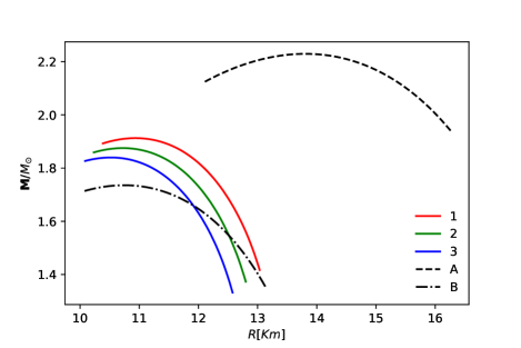
Figure 1: Mass-Radius relations for different EoS

Figure 2: TLN ($\Lambda$) vs Mass (M) for the holographic stars of EoS with the same sets of values and labels for $\ell$ as in Fig. 1.

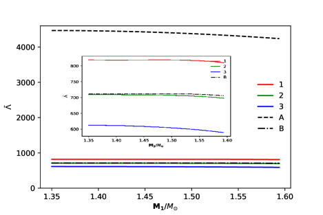
Figure 3: Tidal deformability of the binary holographic stars of EoS vs one of the masses ($\bar{\Lambda}$ vs $\rm{M}_{1}$) for partial sets of the values for $\ell$ used in Fig. 1.

IV IV. Conclusions

The SS model derived from AdS/QCD offers an holographic way to deal with high density nuclear matter, which is difficult in traditional approach. In this letter, we apply the instanton gas structure in SS model to extract the relation between the neutron energy density and the pressure, i.e., the EoS. This is an update for the point-like case in Zhang:2019tqd , with the instanton width $\rho$ as an extra variable. One thing to emphasize is that, $\rho$ is found to be also a function of the chemical potential $\mu$, rather than a free parameter. Thus, the EoS obtained still has only one adjustable parameter, the D8- and $\overline{\rm D8}$-branes separation distance $\ell$. By applying the constraint from GW observation data, especially the binary NS event GW170817 (other NS events offer less sharp windows for TLN), we find that the maximum support mass is about $1.85M_{\odot}$. This value is below the known criterion of known observation of $2M_{\odot}$ NS, but still offer a brand new direction to finally solve the theoretical derivation of EoS in future.

Acknowledgements. The authors thank Prof. Feng-Li Lin and Zhoujian Cao for helpful discussions. KZ (Hong Zhang) is supported by a classified fund from Shanghai city.

Appendix A A. Numerical Calculation Setup

In practice, the process of numerical calculation is constructed as follows. To obtain the pressure $p$ and energy density $\epsilon$ in the EoS, we need to solve the following three equations.

$$0=\int_{0}^{\infty}\frac{2zI_{1}(z,n_{I},\rho,k)}{3(1+z^{2})^{\frac{2}{3}}}\,dz,$$ (15)

$$0=\int_{0}^{\infty}\frac{2zI_{2}(z,n_{I},\rho,k)}{3(1+z^{2})^{\frac{2}{3}}}\,dz,$$ (16)

$$\mu(n_{I},\rho,k)=\int_{0}^{\infty}\frac{2zI_{4}(z,n_{I},\rho,k)}{3(1+z^{2})^{\frac{2}{3}}}\,dz.$$ (17)

Then we can read off

$$p(n_{I},\rho,k)=\frac{2}{7}-\int_{0}^{\infty}\frac{2zI_{5}(z,n_{I},\rho,k)}{3(1+z^{2})^{\frac{2}{3}}}\,dz+\mu(n_{I},\rho,k)\cdot n_{I},$$ (18)

and

$$\epsilon(n_{I},\rho,k)=-\frac{2}{7}+\int_{0}^{\infty}\frac{2zI_{5}(z,n_{I},\rho,k)}{3(1+z^{2})^{\frac{2}{3}}}\,dz.$$ (19)

In which, for the convenience of numerical integration in the equations, we can change the variable $u$ to $z$ with $z$ defined as $u(z)=(1+z^{2})^{\frac{1}{3}}$ before proceeding with the numerical integration.

In Eq. (15)-(19), the functions $I_{i}$ are respectively

$$\begin{split}I_{1}(z,n_{I},\rho,k)=&\left(\frac{3n_{I}\rho^{3}(-4+4u(z)^{3}-\rho^{2})}{8u(z)^{\frac{1}{2}}(-1+u(z)^{3}+\rho^{2})^{\frac{7}{2}}}\right)\\ &\times\left(\frac{u(z)^{4}}{f_{c}(z)\zeta(z,n_{I},\rho,k)}+\zeta(z,n_{I},\rho,k)\right)\\ &-\frac{3n_{I}^{2}f_{c}(z)\rho^{3}u(z)^{3}(-2+2u(z)^{3}+3\rho^{2})}{4u(z)^{\frac{5}{2}}(-1+u(z)^{3}+\rho^{2})^{4}}\\ &\times\frac{\zeta(z,n_{I},\rho,k)}{4u(z)^{\frac{5}{2}}(-1+u(z)^{3}+\rho^{2})^{4}},\end{split}$$ (20)

$$\begin{split}I_{2}(z,n_{I},\rho,k)=&\frac{3n_{I}\rho^{4}}{16u(z)^{\frac{1}{2}}(-1+u(z)^{3}+\rho^{2})^{\frac{7}{2}}}\\ &\times((7+8u(z)^{3}+3\rho^{2})\zeta(z,n_{I},\rho,k)\\ &-\frac{u(z)^{7}(21-11\rho^{2}-21u(z)^{3}+5u(z)^{3}\rho^{2})}{(-1+u(z)^{3})^{2}\zeta(z,n_{I},\rho,k)})\\ &-\frac{3n_{I}^{2}\rho^{4}(u(z)^{3}+2)(-2+2u(z)^{3}+3\rho^{2})}{8u(z)^{\frac{5}{2}}(-1+u(z)^{3}+\rho^{2})^{4}}\\ &\times\frac{\zeta(z,n_{I},\rho,k)}{8u(z)^{\frac{5}{2}}(-1+u(z)^{3}+\rho^{2})^{4}}\\ &-\frac{n_{I}^{\frac{1}{2}}\left(1+\frac{3n_{I}}{4\rho}-k^{2}\right)^{\frac{1}{2}}}{4\rho^{\frac{1}{2}}(u(z)-1)^{\frac{3}{2}}},\end{split}$$ (21)

$$I_{3}(z,n_{I},\rho,k)=\frac{k\zeta(z,n_{I},\rho,k)}{u(z)^{\frac{11}{2}}},$$ (22)

$$\begin{split}I_{4}(z,n_{I},\rho,k)=&\left(\frac{3\rho^{4}}{8u(z)^{\frac{1}{2}}(-1+u(z)^{3}+\rho^{2})^{\frac{5}{2}}}\right)\\ &\times\left(\frac{u(z)^{7}}{(u(z)^{3}-1)\zeta(z,n_{I},\rho,k)}+\zeta(z,n_{I},\rho,k)\right)\\ &+\frac{n_{I}(u(z)^{3}-1)(-2+2u(z)^{3}+3\rho^{2})^{2}}{4u(z)^{\frac{5}{2}}(-1+u(z)^{3}+\rho^{2})^{3}}\\ &\times\frac{\zeta(z,n_{I},\rho,k)}{4u(z)^{\frac{5}{2}}(-1+u(z)^{3}+\rho^{2})^{3}},\end{split}$$ (23)

and

$$\begin{split}I_{5}(z,n_{I},\rho,k)=&-u(z)^{\frac{5}{2}}+u(z)^{\frac{5}{2}}\cdot\zeta(z,n_{I},\rho,k)\\ &\times\left(1+g_{2}(z,n_{I},\rho)+\frac{(n_{I}\cdot Q(z,\rho))^{2}}{u(z)^{5}}\right).\end{split}$$ (24)

The $-u(z)^{\frac{5}{2}}$ term in $I_{5}$, together with the $\frac{2}{7}$ terms in (18) (19), are important, which are introduced to cancel the divergences at infinity. Those do not affect the physical meaning, since the divergent parts never change.

The terms $f_{c}(z)$, $Q(z,\rho)$, $q(z,\rho)$, $g_{1}(z,n_{I},\rho)$, $g_{2}(z,n_{I},\rho)$ and $\zeta(z,n_{I},\rho,k)$ in Eq. (20)-(24) are defined as

$$f_{c}(z)=1-u(z)^{-3},$$ (25)

$$Q(z,\rho)=\frac{(u(z)^{\frac{3}{2}})(f_{c}(z)^{\frac{1}{2}})(3\rho^{2}+2u(z)^{3}-2)}{2((-1+u(z)^{3}+\rho^{2})^{\frac{3}{2}})},$$ (26)

$$q(z,\rho)=\frac{9\cdot u(z)^{\frac{1}{2}}\cdot\rho^{4}}{4\cdot f_{c}(z)^{\frac{1}{2}}\cdot(-1+u(z)^{3}+\rho^{2})^{\frac{5}{2}}},$$ (27)

$$g_{1}(z,n_{I},\rho)=\frac{u(z)^{\frac{1}{2}}\cdot n_{I}\cdot q(z,\rho)}{3\cdot f_{c}(z)^{\frac{1}{2}}},$$ (28)

$$g_{2}(z,n_{I},\rho)=\frac{f_{c}(z)^{\frac{1}{2}}\cdot n_{I}\cdot q(z,\rho)}{3\cdot u(z)^{\frac{7}{2}}},$$ (29)

and

$$\zeta(z,n_{I},\rho,k)=\frac{\left(1+g_{1}(z,n_{I},\rho)\right)^{\frac{1}{2}}}{\left(1+g_{2}(z,n_{I},\rho)-\frac{k^{2}}{u(z)^{8}}+\frac{(n_{I}\cdot Q(z,\rho))^{2}}{u(z)^{5}}\right)^{\frac{1}{2}}}.$$ (30)

Appendix B B. Tidal Love Number

Under Boyer-Lindquist coordinate $(t,r,\theta.\phi)$ 1967JMP…..8..265B , we describe the metric of the sphericlal static NS with

$$ds^{2}=g_{\alpha\beta}^{(0)}dx^{\alpha}dx^{\beta}=-e^{\nu(r)}dt^{2}+e^{\lambda(r)}dr^{2}+r^{2}\left(d\theta^{2}+\sin^{2}\theta d\phi^{2}\right).$$ (31)

Setting $G_{N}=c=1$, $\nu(r)$ and $\lambda(r)$ in the above equation are obtained by $\nu(r)\equiv 2\phi(r)=-\lambda(r)=\ln(1-\frac{2m(r)}{r})$.

The complete metric is combined with the two parts

$$g_{\alpha\beta}=g_{\alpha\beta}^{(0)}+h_{\alpha\beta},$$ (32)

where $h_{\alpha\beta}$ is a linearized metric perturbation.

Under Reege-Wheeler gauge, the perturbation has the expression Hinderer_2009

$$h_{\alpha\beta}=\operatorname{diag}[e^{-\nu(r)}H_{0}(r),e^{\lambda(r)}H_{2}(r),$$

$$r^{2}K(r),r^{2}\sin^{2}\theta K(r)]Y_{2m}(\theta,\varphi).$$ (33)

Here $H_{0}(r)=H_{2}(r)=H(r)$ and $K(r)$ is also related to $H(r)$ by solving perturbative Einstein equation. On the other hand, $H(r)$ can be derived by solving the following equation

$$H^{\prime\prime}+H^{\prime}\left[\frac{2}{r}+e^{\lambda}\left(\frac{2m(r)}{r^{2}}+4\pi r(p-\rho)\right)\right]$$

$$+H\left[-\frac{6e^{\lambda}}{r^{2}}+4\pi e^{\lambda}\left(5\rho+9p+\frac{\rho+p}{(dp/d\rho)}\right)-\nu^{\prime 2}\right]=0,$$ (34)

At the core of NS where $r=0$, $H(r)$ has a solution

$$H(r)=\mathcal{B}r^{2}[1-\frac{2\pi r^{2}}{7}(5\rho(0)+9p(0)+\frac{\rho(0)+p(0)}{(dp/d\rho)(0)})$$

$$+O(r^{3})],$$ (35)

with $\mathcal{B}$ a constant and $dp/d\rho$ depends on the EoS.

At the surface of NS where $r$ is equal to the whole radius $R$, we get the Tidal Love Number

$$k_{2}\equiv\frac{8C^{5}}{5}(1-2C)^{2}[2+2C(y-1)-y]\times$$

$$\{2C(6-3y+3C(5y-8))+4C^{3}[13-11y$$

$$+C(3y-2)+2C^{2}(1+y)]$$

$$+3(1-2C)^{2}[2-y+2C(y-1)]\log(1-2C)\}^{-1}.$$ (36)

Here the compactness of star $C\equiv M/R$ with the total mass $M$. The quantity $y\equiv RH^{\prime}(R)/H(R)$ is set for simplicity in calculation. Actually, we can alternatively start from the evaluation of $Y(r)\equiv rH^{\prime}(r)/H(r)$ directly, then the second order differential equation becomes first order, and easier to solve, as shown in Postnikov:2010yn .

The dimensionless tidal deformability $\Lambda$ is is related to the $l=2$ tidal Love number $k_{2}$ by

$$\Lambda=\frac{2}{3}k_{2}\left(\frac{R}{M}\right)^{5}\text{. }$$ (37)

References

- [1] Ben Margalit and Brian D. Metzger. The Multi-Messenger Matrix: the Future of Neutron Star Merger Constraints on the Nuclear Equation of State. Astrophys. J. Lett., 880(1):L15, 2019.
- [2] Tanja Hinderer. Erratum: “tidal love numbers of neutron stars” (2008, apj, 677, 1216). The Astrophysical Journal, 697(1):964, may 2009.
- [3] James M. Lattimer. The nuclear equation of state and neutron star masses. Ann. Rev. Nucl. Part. Sci., 62:485–515, 2012.
- [4] B. S Sathyaprakash and Bernard F Schutz. Physics, astrophysics and cosmology with gravitational waves. Living Reviews in Relativity, 12(1):2, 2009.
- [5] Duncan Galloway, Feryal Ozel, and Dimitrios Psaltis. Biases for neutron-star mass, radius and distance measurements from Eddington-limited X-ray bursts. Mon. Not. Roy. Astron. Soc., 387:268, 2008.
- [6] Tim Dietrich, Michael W. Coughlin, Peter T. H. Pang, Mattia Bulla, Jack Heinzel, Lina Issa, Ingo Tews, and Sarah Antier. Multimessenger constraints on the neutron-star equation of state and the Hubble constant. Science, 370(6523):1450–1453, December 2020.
- [7] B. P. Abbott et al. Multi-messenger Observations of a Binary Neutron Star Merger. Astrophys. J. Lett., 848(2):L12, 2017.
- [8] B. P. Abbott et al. GW170817: Observation of Gravitational Waves from a Binary Neutron Star Inspiral. Phys. Rev. Lett., 119(16):161101, 2017.
- [9] B. P. Abbott et al. Properties of the binary neutron star merger GW170817. Phys. Rev. X, 9(1):011001, 2019.
- [10] B. P. Abbott et al. GW190425: Observation of a Compact Binary Coalescence with Total Mass . Astrophys. J. Lett., 892(1):L3, 2020.
- [11] Amirhossein Rezaei and Mohammad Parsa Akrami. Exact and Efficient Numerical approaches to MIT Bag Model. 3 2024.
- [12] Kilar Zhang, Takayuki Hirayama, Ling-Wei Luo, and Feng-Li Lin. Compact Star of Holographic Nuclear Matter and GW170817. Phys. Lett. B, 801:135176, 2020.
- [13] Tadakatsu Sakai and Shigeki Sugimoto. More on a holographic dual of QCD. Prog. Theor. Phys., 114:1083–1118, 2005.
- [14] Tadakatsu Sakai and Shigeki Sugimoto. Low energy hadron physics in holographic QCD. Prog. Theor. Phys., 113:843–882, 2005.
- [15] Edward Witten. Anti-de sitter space, thermal phase transition, and confinement in gauge theories. arXiv preprint hep-th/9803131, 1998.
- [16] Joseph Polchinski and Matthew J. Strassler. The String dual of a confining four-dimensional gauge theory. 3 2000.
- [17] Si-wen Li, Andreas Schmitt, and Qun Wang. From holography towards real-world nuclear matter. Physical Review D, 92(2), July 2015.
- [18] Oren Bergman, Gilad Lifschytz, and Matthew Lippert. Holographic Nuclear Physics. JHEP, 11:056, 2007.
- [19] Kazuo Ghoroku, Kouki Kubo, Motoi Tachibana, Tomoki Taminato, and Fumihiko Toyoda. Holographic cold nuclear matter as dilute instanton gas. Phys. Rev. D, 87(6):066006, 2013.
- [20] Kilar Zhang and Feng-Li Lin. Constraint on hybrid stars with gravitational wave events. Universe, 6(12):231, 2020.
- [21] Kilar Zhang, Guo-Zhang Huang, Jie-Shiun Tsao, and Feng-Li Lin. GW170817 and GW190425 as hybrid stars of dark and nuclear matter. Eur. Phys. J. C, 82(4):366, 2022.
- [22] the homogeneous anstaz case does reproduce first order transition, but has no chiral restoration.
- [23] M. J. Duff, B. E. W. Nilsson, and C. N. Pope. Kaluza-Klein Supergravity. Phys. Rept., 130:1–142, 1986.
- [24] Andrea Maselli, Pantelis Pnigouras, Niklas Gronlund Nielsen, Chris Kouvaris, and Kostas D. Kokkotas. Dark stars: gravitational and electromagnetic observables. Phys. Rev. D, 96(2):023005, 2017.
- [25] Kilar Zhang, Ling-Wei Luo, Jie-Shiun Tsao, Chian-Shu Chen, and Feng-Li Lin. Dark stars and gravitational waves: Topical review. Results Phys., 53:106967, 2023.
- [26] Robert H. Boyer and Richard W. Lindquist. Maximal Analytic Extension of the Kerr Metric. Journal of Mathematical Physics, 8(2):265–281, February 1967.
- [27] Sergey Postnikov, Madappa Prakash, and James M. Lattimer. Tidal Love Numbers of Neutron and Self-Bound Quark Stars. Phys. Rev. D, 82:024016, 2010.