Functional Bilevel Optimization for Machine Learning

Abstract

In this paper, we introduce a new functional point of view on bilevel optimization problems for machine learning, where the inner objective is minimized over a function space. These types of problems are most often solved by using methods developed in the parametric setting, where the inner objective is strongly convex with respect to the parameters of the prediction function. The functional point of view does not rely on this assumption and notably allows using over-parameterized neural networks as the inner prediction function. We propose scalable and efficient algorithms for the functional bilevel optimization problem and illustrate the benefits of our approach on instrumental regression and reinforcement learning tasks, which admit natural functional bilevel structures.

1 Introduction

Bilevel optimization is a class of methods for solving optimization problems with a hierarchical structure [Von Stackelberg, 2010]. These problems typically require optimizing the parameters of two interdependent objectives, an inner-level objective $L_{in}$ and an outer-level objective $L_{out}$. The hierarchical structure arises by taking into account the dependence of the inner-level solution on the outer-level variable. Introduced in machine learning for model selection by Bennett et al. [2006] and later for sparse feature learning [Mairal et al., 2012], gradient-based bilevel optimization methods have recently gained a lot of attraction [Feurer and Hutter, 2019, Lorraine et al., 2019, Franceschi et al., 2017] as they offer an alternative to computationally expensive grid search procedures for multiple hyper-parameter tuning. Since then, numerous new applications have emerged, such as meta-learning [Bertinetto et al., 2019], auxiliary task learning [Navon et al., 2021], reinforcement learning [Hong et al., 2023, Liu et al., 2021a, Nikishin et al., 2022], inverse problems [Holler et al., 2018] and invariant risk minimization [Arjovsky et al., 2019, Ahuja et al., 2020].

Bilevel problems are notoriously challenging to solve, even in the most favorable well-defined bilevel setting, where the inner-level problem admits a unique solution. These challenges arise due to the need for approximating both an inner-level solution and its sensitivity to the outer-level variable when performing gradient-based optimization. Several methods, intended for the well-defined setting were devised to address these challenges, such as Iterative Differentiation (ITD, Baydin et al., 2017), or Approximate Implicit Differentiation (AID, Ghadimi and Wang, 2018), often resulting in scalable algorithms with strong convergence guarantees [Domke, 2012, Gould et al., 2016, Ablin et al., 2020, Arbel and Mairal, 2022a, Blondel et al., 2022, Liao et al., 2018, Liu et al., 2022, Shaban et al., 2019].

The well-defined bilevel setting allows devising provably efficient algorithms. However, it typically requires the inner-level objective to be strongly convex. This assumption is often limiting for modern machine learning applications where the inner-level variables are the parameters of a neural network. In these cases, the inner-level problem can possess multiple solutions, making the dependence on the outer-level variable ambiguous [Liu et al., 2021b]. In principle, considering amended versions of the bilevel problem can resolve such an ambiguity. This is the case of optimistic/pessimistic versions of the problem, often considered in the literature on mathematical optimization, where the outer-level objective is optimized over both outer and inner variables, under the optimality constraint of the inner-level variable [Dempe et al., 2007, Ye and Ye, 1997, Ye and Zhu, 1995, Ye et al., 1997]. While tractable methods were recently proposed to solve them [Liu et al., 2021a, b, 2023, Kwon et al., 2024], it is unclear how well would the resulting solutions behave on unseen data in the context of machine learning. For instance, when using an over-parameterized models for the inner-level problem, their parameters must be further optimized for the outer-level objective, possibly resulting in over-fitting [Vicol et al., 2021]. More recently, Arbel and Mairal [2022b] proposed a game formulation involving a selection map to deal with multiple inner-level solutions. Such a formulation justifies the use of ITD/AID outside the well-defined bilevel setting, by viewing those methods as approximations to the Jacobian of the selection map. However, the resulting justifications only hold under rather strong geometric assumptions.

In this work, we identify a functional structure that often arises in bilevel optimization for machine learning problems, and propose a method exploiting this structure to bypass many of the challenges mentioned above. We start from the observation that many bilevel problems arising in machine learning involve an inner-level objective $L_{in}$ that is optimized to learn a model, approximating some optimal prediction function, that is then provided to the outer-level objective $L_{out}$. Furthermore, the inner-level objective is often strongly convex in the outputs of the prediction function (e.g., the mean squared error) even though it might be non-convex as a function of model parameters. These observations enable us to view the machine learning model, typically a neural network, as a function approximation tool within a larger functional space where the bilevel formulation is well defined without the need for strong convexity with respect to model parameters. Formally, we consider bilevel problems involving a prediction function $h$ optimized by the inner-level problem over a Hilbert space $\mathcal{H}$ of functions defined over an input space $\mathcal{X}$ and taking values in a finite dimensional vector space $\mathcal{V}$. The optimal prediction function is then evaluated in the outer level to optimize an outer-level parameter $\omega$ in a finite dimensional space $\Omega=\mathbb{R}^{d}$ giving rise to the following functional bilevel structure:

$$\begin{split}\min_{\omega\in\Omega}\ \mathcal{F}(\omega):&=L_{out}\left(\omega,h^{\star}_{\omega}\right)\\ \text{s.t. }h^{\star}_{\omega}&=\operatorname*{arg\,min}_{h\in\mathcal{H}}\ L_{in}\left(\omega,h\right).\end{split}$$ (FBO)

The inner-level objective $L_{in}$ is assumed to be strongly convex in the prediction function $h$ for any outer-parameter value $\omega$, thus ensuring the uniqueness of the solution $h_{\omega}^{\star}$. The outer-level objective depends on the outer parameter $\omega$ and the optimal prediction function $h^{\star}_{\omega}$, which implicitly depends on the outer parameter $\omega$. The strong convexity assumption with respect to the prediction function is much weaker than the strong convexity assumption with respect to model parameters made in classical bilevel formulations for machine learning, and often holds in practice. For instance, consider a supervised prediction task with pairs of features/labels $(x,y)$ drawn from some empirical training data distribution, formulated as a regularized empirical minimization problem:

$$\min_{h\in\mathcal{H}}L_{in}(\omega,h):={\mathbb{E}}_{x,y}\left[\|y-h(x)\|_{2}^{2}\right]+\omega R(h),$$ (1)

where $\mathcal{H}$ is the space of square integrable functions w.r.t. the distribution of $x$, whereas $R$ is a strongly convex regularization function (e.g. $R(h)=\left\lVert h\right\rVert_{\mathcal{H}}^{2}$) and $\omega$ is a positive outer parameter controlling the amount of regularization. The strong convexity of the regularization in $\mathcal{H}$ ensures that the inner-level objective $L_{in}$ is also strongly convex with respect to $h$. Nonetheless, the optimal prediction function $h_{\omega}^{\star}$ can be a highly nonlinear function of the input $x$, that may be approximated, for instance, by an overparameterized deep neural network. This is the first work to propose a functional point of view that can leverage deep networks for function approximation. The closest works are either restricted to kernel methods [Rosset, 2008, Kunapuli et al., 2008] and thus cannot be used for deep learning models, or propose abstract algorithms that can only be implemented for finite Hilbert spaces [Suonperä and Valkonen, 2024].

We propose an efficient algorithm to solve bilevel problems with the inner objective similar to Equation 1. More precisely, we present a method to solve (FBO) when both outer and inner objectives can be expressed as expectations over data of some point-wise objectives that only require access to the outputs of a prediction function $h$. Additionally, the inner objective is assumed to be strongly convex in the output of the prediction function. This setting covers many problems in machine learning, where the prediction function $h$ belongs to a Hilbert space of square-integrable functions (see Sections 5.1, 5.2, and Appendix A). Our method uses a functional version of the implicit function theorem [Ioffe and Tihomirov, 1979], and the adjoint sensitivty method [Pontryagin, 2018], to derive an expression of the total gradient $\nabla\mathcal{F}(\omega)$. The resulting expression involves an adjoint function $a_{\omega}^{\star}$ that captures the constraints imposed on the optimal inner prediction function. The adjoint $a_{\omega}^{\star}$ is obtained by solving a regression problem in $\mathcal{H}$ corresponding to a well-defined functional linear system. Both the prediction and the adjoint functions can be approximated using parametric models, such as neural networks, that are learned using standard optimization tools, resulting in scalable and efficient algorithms. The proposed method, functional implicit differentiation (FuncID), can be viewed as a functional version of AID, albeit the functional point of view provides advantages that are absent in the original method. AID approximates the solution of a finite dimensional linear system, which involves second order derivatives of the inner objective with respect to the parameters of the model approximating the prediction function $h$. Such a linear system might be ill-posed when the inner objective is non-convex in the model parameters, thus resulting in instabilities [Arbel and Mairal, 2022b]. Instead, FuncID only requires second order information with respect to the output of $h$ to solve the functional linear system. Our method leverages the strong convexity of the inner objective in the output of $h$ to obtain well-defined solutions while also reducing time and memory cost.

Before describing the FuncID method, we discuss some related works in Section 2, and present a theoretical framework for functional implicit differentiation in an abstract Hilbert space $\mathcal{H}$ in Section 3, before specializing it to the common scenario in machine learning, where the Hilbert space $\mathcal{H}$ is an $L_{2}$ space and the objectives are expectations of suitable point-wise losses. In Section 4, we present the FuncID algorithm and illustrate it experimentally on instrumental regression and reinforcement learning tasks in Section 5.

2 Related Work

Bilevel optimization in machine learning.

Two families of bilevel methods are prevalent in machine learning literature due to their scalability: iterative (or “unrolled”) differentiation (ITD, Baydin et al., 2017) and Approximate Implicit Differentiation (AID, Ghadimi and Wang, 2018). ITD approximates the optimal inner-level solution using an ”unrolled” function obtained by applying a sequence of differentiable optimization steps. The outer variable is then optimized by back-propagation through all or parts of these steps to minimize the outer objective [Shaban et al., 2019, Bolte et al., 2024]. When the inner-level is strongly convex, the approximation error of the gradient is known to decrease linearly with the number of optimization steps, albeit at an increased computational and memory cost [Grazzi et al., 2020, Theorem 2.1]. ITD is popular, both in the context of bilevel problems [Grazzi et al., 2020, Marrie et al., 2023] and back-propagation-through-time (BPTT) algorithms [Williams and Peng, 1990], for its simplicity and availability in main deep learning libraries [Bradbury et al., 2018]. However, instabilities in the optimization process are known to arise, especially when the inner-level objective is non-convex [Pascanu et al., 2013, Bengio et al., 1994, Arbel and Mairal, 2022b]. The second approach, AID, uses the Implicit Function Theorem (IFT) to derive the Jacobian of the inner-level solution with respect to the outer variable [Lorraine et al., 2019, Pedregosa, 2016]. It involves (approximately) solving a finite-dimensional linear system to find an adjoint vector representing the optimality constraints imposed on the inner-level solution. AID leverages the hierarchical structure of the bilevel problem through the IFT and offers strong convergence guarantees when the inner objective is smooth and strongly convex [Ji et al., 2021, Arbel and Mairal, 2022a]. However, without strong convexity, the resulting linear system might become ill-posed, as it depends on the possibly degenerate Hessian of the the inner objective with respect to the inner level variables. Degeneracy of the Hessian can occur when the inner variables represent parameters of an overparameterized deep neural network, a common scenario in machine learning that can result in instabilities when using AID. By contrast, our proposed approach does not suffer from this issue even when employing deep networks for function approximation.

Adjoint sensitivity method.

The adjoint sensitivity method [Pontryagin, 2018] is a general technique used to efficiently differentiate a controlled variable with respect to a control parameter. In bilevel optimization, AID can be seen as a direct application of a finite-dimensional version of the adjoint method [Margossian and Betancourt, 2021, Section 2]. Infinite-dimensional versions have also been considered to differentiate solutions of ordinary differential equations [Margossian and Betancourt, 2021, Section 3] with respect to some parameter defining these solutions. In particular, it has been recently exploited in machine learning for optimizing the parameters of a vector field describing an ordinary differential equation (ODE) [Chen et al., 2018]. There, the vector field of the ODE is parameterized by a neural network that is optimized to generate a dynamical system matching some observations. The adjoint sensitivity method provides an efficient alternative to the costly and unstable process of back-propagation through ODE solvers, when differentiating the dynamical system with respect to the parameters of the vector field defining it. The method only requires solving an adjoint ODE, constructed given the original ODE and the loss function, to compute the gradient updates to the parameters, thus resulting in improved performance [Jia and Benson, 2019, Zhong et al., 2019, Li et al., 2020]. The adjoint method for ODEs has also been recently adapted to meta-learning [Li et al., 2023], where the inner optimization procedure is seen as the evolution of an ODE whose gradients are obtained by the adjoint ODE. In all these works, the infinite-dimensional structure arises from applying the adjoint method to solutions of an ODE, where the solutions are functions of the time variable. In the present work, we also consider an infinite-dimensional version of the adjoint sensitivity method. However, unlike the aforementioned works, the infinite-dimensional structure arises from application of the adjoint method to solutions of general learning problems which are functions of input data rather than a single time variable.

Amortization.

Recently, several methods exploited the idea of amortization to approximately solve bilevel problems [MacKay et al., 2019, Bae and Grosse, 2020]. These methods introduce a parametric model called the hypernetwork [Ha et al., 2017, Brock et al., 2018, Zhang et al., 2019] that is optimized to directly predict the inner-level solution, given the outer-level parameter $\omega$ as input. Amortized methods do not fully exploit the implicit dependence in the two levels of a bilevel problem. Instead, they split the two levels into two independent optimization problems: (1) learning the hyper-network on a neighborhood of the outer-level parameter $\omega$, and (2) doing first-order descent on $\omega$ using the learned hyper-network as a replacement for the optimal inner-level solution. These amortized approaches are unlike ITD, AID, or our functional implicit differentiation method, neither of which explicitly model the parametric dependence between the optimal inner-level solution and the outer level variable $\omega$. Amortization techniques are closer to amortized variational inference [Kingma and Welling, 2014, Rezende et al., 2014], where a parametric model is learned to directly produce approximate samples from a posterior distribution, given an observation, instead of applying costly sampling algorithms for each new observation. In the bilevel framework, amortization methods typically perform well when the inner solution has a simple predictable dependence on the outer-level variable $\omega$ and might fail otherwise [Amos et al., 2023, pages 71-72]. By contrast, the functional implicit differentiation framework can adapt to the complex implicit dependence between the inner solution and the outer-level parameter.

3 Functional Bilevel Optimization

The functional bilevel problem (FBO) requires finding the optimal prediction function $h^{\star}_{\omega}$ by optimizing the inner objective in a Hilbert space $\mathcal{H}$ for each value of the outer-level parameter $\omega$. The optimal solution $h^{\star}_{\omega}$ can then be used for characterizing the local variations of $L_{out}$ at a point $(\omega,h^{\star}_{\omega})$, assuming it is Fréchet differentiable, by evaluating its partial derivatives denoted as $g_{\omega}$ in $\mathbb{R}^{d}$ and $d_{\omega}$ in $\mathcal{H}$:

$$g_{\omega}:=\partial_{\omega}L_{out}(\omega,h^{\star}_{\omega})\qquad d_{\omega}:=\partial_{h}L_{out}\left(\omega,h_{\omega}^{\star}\right).$$ (2)

However, solving (FBO) by using a first-order method further requires characterizing the implicit dependence of the optimal prediction function $h^{\star}_{\omega}$ on the outer-level parameter $\omega$ to evaluate the total gradient $\nabla\mathcal{F}(\omega)$ in $\mathbb{R}^{d}$. Indeed, assuming that $h^{\star}_{\omega}$ is also Fréchet differentiable (this assumption will be discussed later), the gradient $\nabla\mathcal{F}(\omega)$ may be obtained by an application of the chain rule:

$$\nabla\mathcal{F}(\omega)=g_{\omega}+\partial_{\omega}h^{\star}_{\omega}d_{\omega}.$$ (3)

The Fréchet derivative $\partial_{\omega}h^{\star}_{\omega}:\mathcal{H}\to\mathbb{R}^{d}$ is a linear operator acting on functions in $\mathcal{H}$ and measures the sensitivity of the optimal solution on the outer variable. We will refer to this quantity as the “Jacobian” in the rest of the paper. While the expression of the gradient in Equation 3 might seem intractable in general, we will see in Section 4 a class of practical algorithms to estimate it. In the present section, we derive general results that guide the construction of these algorithms, starting with a functional version of implicit differentiation.

3.1 Functional implicit differentiation

Our starting point is to characterize the dependence of $h^{\star}_{\omega}$ on the outer variable. To this end, we rely on the following implicit differentiation theorem (proven in Appendix B) which can be seen as a functional version of the one used in AID [Domke, 2012, Pedregosa, 2016], albeit, under a much weaker strong convexity assumption that holds in most practical cases of interest.

Theorem 3.1 (Functional implicit differentiation).

Consider problem (FBO) and assume that:

• For any $\omega\in\Omega$, there exists $\mu>0$ for which $h\mapsto L_{in}(\omega^{\prime},h)$ is $\mu$-strongly convex for any $\omega^{\prime}$ near $\omega$.

• $h\mapsto L_{in}(\omega,h)$ has finite values and is Fréchet differentiable on $\mathcal{H}$ for all $\omega\in\Omega$.

• $\partial_{h}L_{in}$ is Hadamard differentiable on $\Omega\times\mathcal{H}$ (in the sense of Definition B.1 in Section B.1).

Then, $\omega\mapsto h^{\star}_{\omega}$ is uniquely defined and is Fréchet differentiable with a Jacobian $\partial_{\omega}h^{\star}_{\omega}$ given by:

$$B_{\omega}+\partial_{\omega}h^{\star}_{\omega}C_{\omega}=0,\qquad\text{with }\quad B_{\omega}:=\partial_{\omega,h}L_{in}(\omega,h^{\star}_{\omega}),\quad\text{and}\quad C_{\omega}:=\partial^{2}_{h}L_{in}(\omega,h^{\star}_{\omega}).$$ (4)

Theorem 3.1 provides a formal expression of the Jacobian $\partial_{\omega}h^{\star}_{\omega}$ as the solution of a linear system in the Hilbert space $\mathcal{H}$. The strong convexity assumption on the inner-level objective ensures the existence and uniqueness of the solution $h_{\omega}^{\star}$, while the differentiability assumptions on $L_{in}$ and $\partial_{h}L_{in}$ ensure that the map $\omega\mapsto h_{\omega}^{\star}$ is Fréchet differentiable. Similar conclusions could be obtained by directly applying the implicit function theorem for abstract Banach spaces [see Ioffe and Tihomirov, 1979]. However, such a theorem requires making the stronger assumption that $\partial_{h}L_{in}$ is continuously Fréchet differentiable. This assumption turns our to be quite restrictive, in our setting, as it would only hold for objectives that are quadratic in $h$ (see [Nemirovski and Semenov, 1973, Corollary 2, p 276] and discussions in [Noll, 1993, Goodman, 1971]). To allow more generality, Theorem 3.1 employs the weaker notion of Hadamard differentiability for $\partial_{h}L_{in}$. Hadamard differentiability is widely used in statistics, in particular for deriving the delta-method, as it holds for a much larger class of functionals [van der Vaart and Wellner, 1996, Chapter 3.9], and happens to be the right notion of differentiability in our setting as we further show in Section 4.

Similarly to AID, constructing the full Jacobian $\partial_{\omega}h^{\star}_{\omega}$ can be avoided, since only a Jacobian-vector product is needed when computing the total gradient $\nabla\mathcal{F}(\omega)$. The result in Proposition 3.2 below, relies on the adjoint sensitivity method [Pontryagin, 2018] to provide a more convenient expression for $\nabla\mathcal{F}(\omega)$ and is proven in Section B.2.

Proposition 3.2 (Functional adjoint sensitivity).

Under the same assumption on $L_{in}$ as in Theorem 3.1 and further assuming that $L_{out}$ is jointly differentiable in $\omega$ and $h$, the total objective $\mathcal{F}$ is differentiable with $\nabla\mathcal{F}(\omega)$ given by:

$$\nabla\mathcal{F}(\omega)=g_{\omega}+B_{\omega}a_{\omega}^{\star},$$ (5)

where the adjoint function $a^{\star}_{\omega}:=-C_{\omega}^{-1}d_{\omega}$ is an elemen of $\mathcal{H}$ that minimizes the quadratic objective:

$$a_{\omega}^{\star}=\arg\min_{a\in\mathcal{H}}L_{adj}(\omega,a):=\tfrac{1}{2}\ \langle a,C_{\omega}a\rangle_{\mathcal{H}}+\langle a,d_{\omega}\rangle_{\mathcal{H}}.$$ (6)

The new expression of the total gradient provided by Proposition 3.2 requires finding an adjoint function $a^{\star}$ in $\mathcal{H}$ by optimizing a strongly convex quadratic objective $L_{adj}$ in $\mathcal{H}$. The strong convexity of the adjoint objective $L_{adj}$ guarantees the existence of a unique minimizer and is a direct consequence of the Hessian operator $C_{\omega}$ being positive definite by the strong convexity of the inner-objective in $h$. Equation 5 suggests that, in addition to finding the optimal prediction $h_{\omega}^{\star}$, obtained by solving the inner-level optimization problem, computing the total gradient requires optimizing the quadratic objective (6) to find the adjoint function $a_{\omega}^{\star}$. Both optimization problems occur in the same function space $\mathcal{H}$ and are equivalent in terms of conditioning since their Hessian operators at the optimum are identical.

Connection with parametric implicit differentiation. As shown in Appendix C, it is possible to approximate the functional problem in Equation FBO with a parametric bilevel problem where the inner-level functions are restricted to have a parametric form $h(x)=\tau(\theta)(x)$ with parameters $\theta$. There, the inner-level variable becomes $\theta$ instead of the function $h$ (see Equation PBO of Appendix C). One can then apply standard algorithms for bilevel optimization such as AID which are derived from the parametric version of implicit differentiation and require differentiating twice w.r.t. the parametric model. However, for models such as deep neural networks, the inner objective in the parametric formulation is no longer strongly convex in the inner-variables (the model’s parameters $\theta$), since the parametric Hessian can be non-positive and even degenerate (see Proposition C.1 of Appendix C). The resulting total gradient is, in general, different from the one in Equation 5 (see Proposition C.2 of Appendix C) and can cause numerical instabilities, particularly when using algorithms such as AID for which an adjoint vector is obtained by solving a quadratic problem defined by the parametric Hessian matrix. Moreover, if the model admits multiple solutions, the Hessian is likely to be degenerate making the implicit function theorem inapplicable. On the other hand, the functional implicit differentiation requires finding an adjoint function $a_{\omega}^{\star}$ by solving a positive definite quadratic problem in $\mathcal{H}$ which is always guaranteed to have a solution, even when the inner-level prediction function $h^{\star}_{\omega}$ is approximated by a sub-optimal solution, thanks to the strong convexity of the lower-level objective $h\mapsto L_{in}(\omega,h)$. This stability property w.r.t. sub-optimal solutions is crucial for deriving practical algorithms such as the one presented in Section 4, where the optimal prediction function is approximated within a parametric family, such as neural networks.

3.2 Functional bilevel optimization in $L_{2}$ spaces

We specialize the abstract results in Section 3.1 to a more common situation in machine learning when both inner and outer level objectives of FBO are given as expectations of some point-wise functions over observed data. More precisely, we consider two data distributions $\mathbb{P}$ and $\mathbb{Q}$ defined over a product space $\mathcal{X}\times\mathcal{Y}\subset\mathbb{R}^{d_{x}}\times\mathbb{R}^{d_{y}}$ and denote by $\mathcal{H}$ the Hilbert space of functions $h:\mathcal{X}\rightarrow\mathcal{V}$ that are square integrable under $\mathbb{P}$, where $\mathcal{V}$ is a finite dimensional vector space (i.e. $\mathcal{V}=\mathbb{R}^{d_{v}})$. Given an outer parameter space $\Omega$, we consider the following functional bilevel problem:

$$\begin{split}\min_{\omega\in\Omega}\ L_{out}\left(\omega,h^{\star}_{\omega}\right)&:=\mathbb{E}_{(x,y)\sim\mathbb{Q}}\left[\ell_{out}\left(\omega,h^{\star}_{\omega}(x),x,y\right)\right]\\ \text{s.t. }h^{\star}_{\omega}&=\operatorname*{arg\,min}_{h\in\mathcal{H}}\ L_{in}\left(\omega,h\right):=\mathbb{E}_{(x,y)\sim\mathbb{P}}\left[\ell_{in}\left(\omega,h(x),x,y\right)\right],\end{split}$$ (7)

where $\ell_{out}$, $\ell_{in}$ are point-wise loss functions defined on $\Omega\times\mathcal{V}\times\mathcal{X}\times\mathcal{Y}$ and where the outer expectation is taken w.r.t. $\mathbb{Q}$ while the inner one is w.r.t. $\mathbb{P}$. This setting encompasses a large family of problems in deep learning of which a few are discussed in Sections 5.1 and 5.2, and in Appendix A and is a particular case of Equation FBO. In addition to modelling a large family of prediction functions, the Hilbert space $\mathcal{H}$ of square-integrable functions allows us to obtain more concrete expressions for the the total gradient $\nabla\mathcal{F}(\omega)$, from which we derive practical algorithms in Section 4.

The following proposition, proved in Appendix D, makes mild technical assumptions on $\mathbb{P}$, $\mathbb{Q}$ and $\ell_{in}$ and $\ell_{out}$ provided in Section D.1 to ensure that the conditions on $L_{in}$ and $L_{out}$ in Proposition 3.2 hold and derives expression for the total gradient in the form of expectations under $\mathbb{P}$ and $\mathbb{Q}$.

Proposition 3.3 (Functional Adjoint sensitivity in $L_{2}$ spaces.).

Under Assumptions (B), (C), (D), (E), (F), (G) and (A) on $\ell_{in}$, Assumptions (H), (I) and (J) on $\ell_{out}$ and Assumptions (K) and (L) on $\mathbb{P}$ and $\mathbb{Q}$ stated in Section D.1, the conditions on $L_{in}$ and $L_{out}$ in Proposition 3.2 hold, so that the total gradient $\nabla\mathcal{F}(\omega)$ of $\mathcal{F}$ is expressed as $\nabla\mathcal{F}(\omega)=g_{\omega}+B_{\omega}a_{\omega}^{\star}$ with $a^{\star}_{\omega}\in\mathcal{H}$ being the minimizer of the objective $L_{adj}$ in Equation 6. Moreover, $L_{adj}$, $g_{\omega}$ and ${B}_{\omega}a_{\omega}^{\star}$ admit the following expressions:

$$\begin{split}L_{adj}(\omega,a)=&\tfrac{1}{2}\ \mathbb{E}_{(x,y)\sim\mathbb{P}}\left[a(x)^{\top}\partial_{v}^{2}\ell_{in}\left(\omega,h_{\omega}^{\star}(x),x,y\right)a(x)\right]\\ &+\mathbb{E}_{(x,y)\sim\mathbb{Q}}\left[a(x)^{\top}\partial_{v}\ell_{out}\left(\omega,h_{\omega}^{\star}(x),x,y\right)\right],\end{split}$$ (8)

$$g_{\omega}=\mathbb{E}_{(x,y)\sim\mathbb{Q}}\left[\partial_{\omega}\ell_{out}\left(\omega,h_{\omega}^{\star}(x),x,y\right)\right]\qquad{B}_{\omega}a_{\omega}^{\star}=\mathbb{E}_{(x,y)\sim\mathbb{P}}\left[\partial_{\omega,v}\ell_{in}\left(\omega,h_{\omega}^{\star}(x),x,y\right)a_{\omega}^{\star}(x)\right],$$ (9)

where $\partial_{\omega}\ell_{out}$ and $\partial_{v}\ell_{out}$ are the partial derivatives of $\ell_{out}$ in its first and second arguments (i.e. $\omega$ and $v$), $\partial_{\omega,v}\ell_{in}$ is the cross-derivative of $\ell_{in}$ w.r.t. to $\omega$ and $v$, while $\partial_{v}^{2}\ell_{in}$ is the second-order derivatives of $\ell_{in}$ w.r.t. to $v$.

The assumptions on $\mathbb{P}$ and $\mathbb{Q}$ ensure their second moments are finite and that the marginal of $x$ under $\mathbb{Q}$ has a bounded Radon-Nikodym derivative w.r.t. the marginal of $x$ under $\mathbb{P}$. These are mild requirements to obtain a well-defined problem in Equation 7 by ensuring that square integrable functions under $\mathbb{P}$ are also square integrable under $\mathbb{Q}$. The assumptions on $\ell_{in}$ and $\ell_{out}$ are essentially integrability, differentiability and Lipschitz continuity assumptions on the objectives $\ell_{in}$ and $\ell_{out}$ in addition to the strong convexity of $\ell_{in}$ in its second argument. These assumptions typically hold for objectives such as the squared error or the cross entropy objective as shown in Proposition D.1 of Section D.1.

4 Methods for Functional Bilevel Optimization in $L_{2}$ Spaces

We propose a flexible class of algorithms for solving the functional bilevel problem in $L_{2}$ spaces described in Section 3.2 when samples from distributions $\mathbb{P}$ and $\mathbb{Q}$ are available. We call the method Functional Implicit Differentiation (FuncID) and provide its general structure in Algorithm 1. FuncID relies on three main components:

1. Empirical objectives. These approximate the three population objectives $L_{out}$, $L_{in}$ and $L_{adj}$ as empirical expectations over samples from inner and outer datasets $\mathcal{D}_{in}$ and $\mathcal{D}_{out}$, distributed according to $\mathbb{P}$ and $\mathbb{Q}$.

2. Function approximation. The search space for both the prediction and adjoint functions is restricted to parametric spaces with finite-dimensional parameters $\theta$ and $\xi$. Approximate solutions $\hat{h}_{\omega}$ and $\hat{a}_{\omega}$ to the optimal functions $h_{\omega}^{\star}$ and $a_{\omega}^{\star}$ are obtained using standard optimization procedures over the empirical objectives.

3. Total gradient approximation. FuncID estimates the total gradient $\nabla\mathcal{F}(\omega)$ using the empirical objectives, and the approximations $\hat{h}_{\omega}$ and $\hat{a}_{\omega}$ of the prediction and adjoint functions.

Sections 4.1, 4.2 and 4.3 present the three components of FuncID while Section 4.4 discusses its computational cost.

Algorithm 1 FuncID

Input: initial outer parameter $\omega_{0}$, initial parameters $\theta_{0}$ of the inner model, and $\xi_{0}$ of the adjoint model

for $n=0,\ldots,N-1$ do

      # Inner-level optimization

     $\hat{h}_{\omega_{n}},\theta_{n+1}\leftarrow$ InnerOpt($\omega_{n},\theta_{n},\mathcal{D}_{in}$)

      # Adjoint optimization

     Sample a mini-batch $\mathcal{B}=(\mathcal{B}_{out},\mathcal{B}_{in})$ from $\mathcal{D}=(\mathcal{D}_{out},\mathcal{D}_{in})$

     $\hat{a}_{\omega_{n}},\xi_{n+1}\leftarrow$ AdjointOpt($\omega_{n},\xi_{n},\hat{h}_{\omega_{n}},\mathcal{B}$)

      # Outer gradient estimation

     $g_{out}\leftarrow$ TotalGrad($\omega_{n},\hat{h}_{\omega_{n}},\hat{a}_{\omega_{n}},\mathcal{B}$)

     $\omega_{n+1}\leftarrow$ update $\omega_{n}$ using $g_{out}$

end for

4.1 From population losses to empirical objectives

We assume that we have access to two datasets $\mathcal{D}_{in}$ and $\mathcal{D}_{out}$ consisting of pairs of samples $(x,y)$ in $\mathcal{D}_{in}$ and $(\tilde{x},\tilde{y})$ in $\mathcal{D}_{out}$ that we use to define an empirical version of the population objectives in Equation 7. We may assume, for simplicity, that the samples are i.i.d. samples of $\mathbb{P}$ and $\mathbb{Q}$, respectively. However, such an assumption may be relaxed, for instance, when using samples from a Markov chain or a Markov Decision Process, which can still be used to approximate the population objectives. Additionally, if $\mathbb{P}$ and $\mathbb{Q}$ are very similar, the two datasets might be equal or be two separate sets as long as they provide a good approximation to the population distributions. For scalability in the size of datasets, we consider a mini-batch setting where batches of data $\mathcal{B}=\left(\mathcal{B}_{out},\mathcal{B}_{in}\right)$ are sub-sampled from datasets $\mathcal{D}:=\left(\mathcal{D}_{out},\mathcal{D}_{in}\right)$ and used to define the approximate objectives.

Approximating both inner and outer level objectives in Equation 7 is straightforward and can be done, for instance, using the following empirical versions:

$$\hat{L}_{out}\left(\omega,h,\mathcal{B}_{out}\right) :=\tfrac{1}{\left\lvert\mathcal{B}_{out}\right\rvert}\sum_{(\tilde{x},\tilde{y})\in\mathcal{B}_{out}}\ell_{out}\left(\omega,h(\tilde{x}),\tilde{x},\tilde{y}\right)$$

$$\hat{L}_{in}\left(\omega,h,\mathcal{B}_{in}\right) :=\tfrac{1}{\left\lvert\mathcal{B}_{in}\right\rvert}\sum_{(x,y)\in\mathcal{B}_{in}}\ell_{in}\left(\omega,h(x),x,y\right).$$

Adjoint objective. Using the expression of $L_{adj}$ from Proposition 3.3, we derive a finite-sample approximation of the adjoint loss by replacing the population expectations by their empirical counterparts. More precisely, assuming we have access to an approximation $\hat{h}_{\omega}$ to the inner-level prediction function obtained by a procedure that we describe later in Section 4.2, we consider the following empirical version of the adjoint objective:

$$\begin{split}\hat{L}_{adj}\left(\omega,a,\hat{h}_{\omega},\mathcal{B}\right):=&\tfrac{1}{2}\tfrac{1}{\left\lvert\mathcal{B}_{in}\right\rvert}\sum_{(x,y)\in\mathcal{B}_{in}}a(x)^{\top}\partial_{v}^{2}\ell_{in}(\omega,\hat{h}_{\omega}(x),x,y)\ a(x)\\ &+\tfrac{1}{\left\lvert\mathcal{B}_{out}\right\rvert}\sum_{(x,y)\in\mathcal{B}_{out}}a(x)^{\top}\partial_{v}\ell_{out}\left(\omega,\hat{h}_{\omega}(x),x,y\right).\end{split}$$ (10)

The adjoint objective in Equation 10 requires computing a Hessian-vector product with respect to the output $v$ of the prediction function $\hat{h}_{\omega}$. Meanwhile, AID methods necessitate a Hessian-vector product with respect to the parameters of a parameterized version of $\hat{h}_{\omega}$, which are usually of a much higher dimension then $v$. We detail the computational cost differences of FuncID and AID in Section 4.4.

4.2 Approximate prediction and adjoint functions

To find approximate solutions to the prediction and adjoint functions we rely on three steps: 1) specifying parametric search spaces for both functions, 2) introducing optional regularization to prevent overfitting and, 3) defining a gradient-based optimization procedure using the approximate objectives defined in Section 4.1.

Parametric search space.

We approximate both prediction and adjoint functions using parametric search spaces. We consider a parametric family of functions defined by a map $\tau:\Theta\rightarrow\mathcal{H}$ over a set of parameters $\Theta\subseteq\mathbb{R}^{p_{in}}$. We then constrain the prediction function $h$ to be a model of the form $h(x)=\tau(\theta)(x)$. We only need $\tau$ to be continuous and differentiable almost everywhere so that back-propagation is applicable [Bolte et al., 2021]. Importantly, we do not require twice differentiability of $\tau$, as AID would, because the Hessian in functional implicit differentiation is computed w.r.t. the output of $\tau$, and not w.r.t. its parameters. To allow for more generality, we can consider a different parameterized model $\nu:\Xi\rightarrow\mathcal{H}$ for approximating the adjoint function, which is defined over a possibly different set of parameters $\Xi\subseteq\mathbb{R}^{p_{adj}}$. We then constrain the adjoint to be of the form $a(x)=\nu(\xi)(x)$. Again, we require it to be continuous and differentiable almost everywhere. In practice, we use the same parameterization, typically a neural network, for both the inner-level and the adjoint models.

Regularization.

With the empirical objectives and parametric search spaces defined earlier, we can directly optimize the parameters of both the inner-level model $\tau$ and the adjoint model $\nu$. However, due to finite samples, it is often desirable to introduce a regularization to these empirical objectives to obtain approximations that generalize better to unseen data. The method does not impose any constraint on the choice of the regularization, as it is simply introduced to account for finite samples effect. Therefore, we may regularize both inner and outer objectives using functions $\theta\mapsto R_{in}(\theta)$ and $\xi\mapsto R_{adj}(\xi)$ such as the ridge penalty or any other commonly used regularization.

Optimization.

All the operations that require differentiation in FuncID, including Hessian-vector products, and learning the models $\tau(\theta)$ and $\nu(\xi)$, can be implemented using standard optimization procedures leveraging automatic differentiation packages such as Pytorch [Paszke et al., 2019] or Jax [Bradbury et al., 2018]. The function InnerOpt($\omega,\theta_{0},\mathcal{D}_{in}$) defined in Algorithm 2 optimizes the parameters of the inner model for a given value of $\omega$, initialization $\theta_{0}$ and data $\mathcal{D}_{in}$. The optimization procedure consists of $M$ gradient updates to the inner model’s parameters using any standard optimizer. The algorithm then returns a pair of optimized parameters $\theta_{M}$ and the corresponding inner model $\tau(\theta_{M})$, the latter being the approximate solution to the inner-level problem, i.e. $\hat{h}_{\omega}=\tau(\theta_{M})$. Similarly, AdjointOpt($\omega,\xi_{0},\hat{h}_{\omega_{n}},\mathcal{B}$) defined in Algorithm 3 optimizes the adjoint model’s parameters in the same way as Algorithm 2 with $K$ gradient updates and whose output defines the approximate adjoint function $\hat{a}_{\omega}=\nu(\xi_{K})$. Other optimization procedures can be used for finding the adjoint function especially for some particular losses and model choices for which closed-form solutions are possible to obtain, as we exploit in some of our experiments in Section 5.

Algorithm 2  InnerOpt($\omega,\theta_{0},\mathcal{D}_{in}$) $\hat{h}_{\omega}$

for $m=0,\ldots,M-1$ do

     Sample batch $B_{in}$ from $\mathcal{D}_{in}$

     $g_{in}\leftarrow\nabla_{\theta}\hat{L}_{in}\left(\omega,\tau(\theta_{m}),\mathcal{B}_{in}\right)+\nabla_{\theta}R_{in}(\theta_{m})$

     $\theta_{m+1}\leftarrow$ Update $\theta_{m}$ using $g_{in}$

end for

Return $\tau(\theta_{M}),\theta_{M}$

Algorithm 3  AdjointOpt($\omega,\xi_{0},\hat{h}_{\omega},\mathcal{B}$)

for $k=0,\ldots,K-1$ do

     $g_{adj}\leftarrow\nabla_{\xi}\ \hat{L}_{adj}\left(\omega,\nu(\xi_{t}),\hat{h}_{\omega},\mathcal{B}\right)+\nabla_{\xi}R_{adj}(\xi_{k})$

     $\xi_{k+1}\leftarrow$ Update $\xi_{k}$ using $g_{adj}$

end for

Return $\nu(\xi_{K}),\xi_{K}$

4.3 Total gradient estimation

We provide the algorithmic steps for estimating the theoretical total gradient $\nabla\mathcal{F}(\omega)$. We exploit Proposition 3.3 to derive Algorithm 4, which allows us to approximate the total gradient using observed data points, after computing the approximate solutions $\hat{h}_{\omega}$ and $\hat{a}_{\omega}$. Algorithm 4 defines a function  TotalGrad($\omega,\hat{h}_{\omega},\hat{a}_{\omega},\mathcal{B}$) for approximating the total gradient $\nabla\mathcal{F}(\omega)$ given approximations $\hat{h}_{\omega},\hat{a}_{\omega}$ and a batch of data $\mathcal{B}$. There, we decompose the gradient into two terms: $g_{Exp}$, an empirical approximation of $g_{\omega}$ in Equation 9 using the approximations $\hat{h}_{\omega}$ and representing the explicit dependence of the outer variable $\omega$ on $\hat{L}_{out}$, and $g_{Imp}$, an approximation to the implicit gradient term $B_{\omega}a_{\omega}^{\star}$ in Equation 9. The term $g_{Imp}$ is simply obtained by replacing the expectation in Equation 9 by an empirical average over a batch $\mathcal{B}_{in}$ of inner-level data, and using the approximations $\hat{h}_{\omega}$ and $\hat{a}_{\omega}$ instead of the exact solutions.

Algorithm 4  TotalGrad($\omega,\hat{h}_{\omega},\hat{a}_{\omega},\mathcal{B}$)

$g_{Exp}\leftarrow\partial_{\omega}\hat{L}_{out}\left(\omega,\hat{h}_{\omega},\mathcal{B}_{out}\right)$

$g_{Imp}\leftarrow\frac{1}{\left\lvert\mathcal{B}_{in}\right\rvert}\sum_{(x,y)\in\mathcal{B}_{in}}\partial_{\omega,v}\ell_{in}(\omega,\hat{h}_{\omega}(x),x,y)\ \hat{a}_{\omega}(x)$

Return $g_{Exp}+g_{Imp}$

4.4 Computational cost and scalability

Algorithm 1 has a double loop structure similar to AID, where the inner loops sequentially update the prediction and adjoint models using scalable algorithms such as stochastic gradient descent [Robbins and Monro, 1951, Bottou, 2010]. It employs a warm-start procedure, which consists of initializing both model parameters for each new outer-level iteration using the ones obtained at the previous iteration. A similar warm-start strategy is provably known to be beneficial in the case of AID [Arbel and Mairal, 2022a] and was also empirically useful in our experiments.

The optimization of the prediction function $\hat{h}_{\omega}$ in the inner-level optimization loop is similar to AID, although the total gradient computation differs significantly. Unlike AID, Algorithm 1 does not require differentiating through the parameters of the prediction model when estimating the total gradient $\nabla\mathcal{F}(\omega)$. This property results in an improved cost in time and memory in most practical cases as shown in Table 1 and Figure 1. More precisely, AID requires computing Hessian-vector products of size $p_{in}$, which corresponds to the number of hidden layer weights of the neural network $\hat{h}_{\omega}$. While FuncID only requires Hessian-vector products of size $d_{v}$, i.e. the output dimension of $\hat{h}_{\omega}$. In many practical cases, the network’s parameter dimension $p_{in}$ is much larger than its output size $d_{v}$, which results in considerable benefits in terms of memory when using FuncID rather than AID, as shown in Figure 1 (left). Furthermore, unlike AID, the overhead of evaluating Hessian-vector products in FuncID is not affected by the time cost for evaluating the prediction network. When $\hat{h}_{\omega}$ is a deep network, such an overhead increases significantly with the network size, making AID significantly slower (Figure 1 (right)).

$$\begin{array}[]{lccc}\hline\cr\text{ Method }&\text{ Time cost}&\text{ Memory cost}\\ \hline\cr\text{AID}&\gamma(T_{L_{in}}+T_{h})&\beta p_{in}+M_{h}\\ \text{\emph{FuncID}}&\gamma T_{L_{in}}+(2+\delta)T_{a}+T_{h}&\beta d_{v}+M_{a}\\ \hline\cr\end{array}$$

Table 1: Cost in time and memory for performing a single total gradient estimation using either AID or FuncID and assuming the prediction model is learned. Time cost: $T_{h}$ and $T_{a}$ represent the time cost of evaluating both prediction and adjoint models $h$ and $a$, while $T_{in}$ is the time cost for evaluating the inner objective once the outputs of $h$ are computed. The factors $\gamma$ and $\delta$ are multiplicative overheads for evaluating hessian-vector products and gradient. Memory cost: $M_{h}$ and $M_{a}$ represent the memory cost of storing the intermediate outputs of $h$ and $a$, $p_{in}$ and $d_{v}$ are the memory costs of storing the Hessian-vector product for AID and FuncID respectively and $\beta$ is a multiplicative constant that depends on a particular implementation.

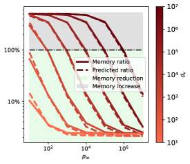
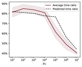
Figure 1: Memory and time comparison of a single total gradient approximation using FuncID vs AID. (Left) Memory usage ratio of FuncID over AID vs inner model parameter dimension $p_{in}$, for various values of the output dimension $d_{v}$. (Right) Time ratio of FuncID over AID vs inner model parameter dimension $p_{in}$ averaged over several values of $d_{v}$ and $10^{4}$ evaluations. The continuous lines are experimental results obtained using a JAX implementation [Bradbury et al., 2018] running on a GPU. The dashed lines correspond to theoretical estimates obtained using the algorithmic costs given in Table 1 with $\gamma=12,\delta=2$ for time, and the constant factors in the memory cost fitted to the data.

5 Applications

We consider two applications of the functional bilevel optimization problem: two stage least squares regression (2SLS) and model-based reinforcement learning. To illustrate its effectiveness we compare it with other approaches to bilevel optimization such as AID or ITD as well as state-of-the-art methods for each of the considered applications. We provide a general implementation of FuncID in PyTorch [Paszke et al., 2019] and use it for the 2SLS application. Our implementation is compatible with any standard optimizer (such as Adam [Kingma and Ba, 2015]) and supports standard regularization techniques. For the reinforcement learning application, we leverage an existing implementation in JAX [Bradbury et al., 2018] of the model-based RL from Nikishin et al. [2022] and build on it to apply funcID. To ensure fair comparison, we conduct experiments with comparable computational budgets for hyper-parameter tuning of all methods. Moreover, we use the same neural network architectures for all methods and repeat the experiments multiple times with different random seeds.

5.1 Two-stage least squares regression (2SLS)

Two-stage least squares regression is a class of methods often encountered in causal representation learning such as instrumental regression or proxy causal learning [Stock and Trebbi, 2003]. 2SLS was recently addressed using bilevel optimization approaches showing promising results [Xu et al., 2021b, a, Hu et al., 2023]. We focus on 2SLS for Instrumental Variable (IV) regression as it is a widely-used statistical framework for handling endogeneity in econometrics [Blundell et al., 2007, 2012], medical economics [Cawley and Meyerhoefer, 2012], sociology [Bollen, 2012], and, recently, for handling confounders in off-line reinforcement learning [Fu et al., 2022].

Figure 2: The causal relationships between all variables in an Instrumental Variable (IV) causal graph, where $t$ is the treatment variable (dsprites image), $o$ is the outcome (label in $\mathbb{R}$), $x$ is the instrument and $\epsilon$ is the unobserved confounder

Problem formulation.

In an IV problem, the goal is to learn a model $f_{\omega}:t\mapsto o$ that approximates the true structural function $f_{struct}$ using independent samples $(o,t,x)$ from a data distribution $\mathbb{P}$, where $x$ is an instrumental variable. The function $f_{struct}$ describes the true effect of a treatment $t$ on an outcome $o$. The main challenge in IV is the existence of an unobserved confounder $\epsilon$ influencing both $t$ and $o$ additively and making the recovery of $f_{\omega}$ using standard regression impossible Figure 2. Instead, if the instrumental variable $x$ affects the outcome $o$ only through the treatment $t$ and is independent from the confounder $\epsilon$, one can use it to recover the direct relationship between the treatment $t$ and the outcome $o$ using the 2SLS framework under a mild assumption on the confounder [Singh et al., 2019]. The regression problem is then replaced by a variant that averages the effect of the treatment $t$ conditionally on $x$:

$$\min_{\omega\in\Omega}\mathbb{E}_{\mathbb{P}}\left[\left\lVert o-\mathbb{E}_{\mathbb{P}}\left[f_{\omega}(t)|x\right]\right\rVert^{2}\right].$$ (11)

Directly estimating the conditional expectation $\mathbb{E}_{\mathbb{P}}\left[f_{\omega}(t)|x\right]$ is hard in general. Instead, it is easier to express it, equivalently, as the solution of another regression problem predicting $f_{\omega}(t)$ from $x$:

$$h_{\omega}^{\star}:=\mathbb{E}_{\mathbb{P}}\left[f_{\omega}(t)|x\right]=\arg\min_{h\in\mathcal{H}}\mathbb{E}_{\mathbb{P}}\left[\left\lVert f_{\omega}(t)-h(x)\right\rVert^{2}\right].$$ (12)

Both equations result in the bilevel formulation in Equation 7 with $y=(t,o)$, $\mathbb{Q}=\mathbb{P}$ and the point-wise losses $\ell_{in}$ and $\ell_{out}$ given by $\ell_{in}(\omega,v,x,y)=\ell_{in}(\omega,v,x,(t,o))=\left\lVert f_{\omega}(t)-v\right\rVert^{2}$ and $\ell_{out}(\omega,v,x,y)=\ell_{out}(\omega,v,x,(t,o))=\left\lVert o-v\right\rVert^{2}$. It is, therefore, possible to directly apply Algorithm 1 to learn $f_{\omega}$ as we illustrate below.

Experimental setup.

We solve a benchmark IV problem on the dsprites dataset [Matthey et al., 2017], a collection of synthetic images each representing a single object generated using five latent parameters: shape, scale, rotation, and posX, posY positions on the image coordinates. In this setting, the treatment variable $t$ are the images, the hidden confounder $\epsilon$ is the second coordinate posY, while the other four latent variables form the instrumental variable $x$. The outcome $o$ is some predefined but unknown structural function $f_{struct}$ of $t$ that is contaminated by the confounder $\epsilon$ as described in Section E.1. We closely follow the setting of Deep Feature Instrumental Variable Regression (DFIV) dsprites experiment described by Xu et al. [2021a, Section 4.2], which reports state-of-the-art performance. There, the prediction function and the structural model are neural networks that are optimized to solve the bilevel problem in Equations 11 and 12. We consider two versions of our method to solve this problem, both of which use an adjoint network that has the same architecture as the inner prediction function: FuncID, which optimizes all parameters of the adjoint network and FuncID linear, which only learns the last layer in closed-form while setting the hidden layer parameters to those of the inner prediction function. We then compare our method with DFIV, AID and ITD using the same network architectures and the same computational budget for selecting hyper-parameters. Full details on the network architectures, hyperparameters and the training setting are described in Section E.2.

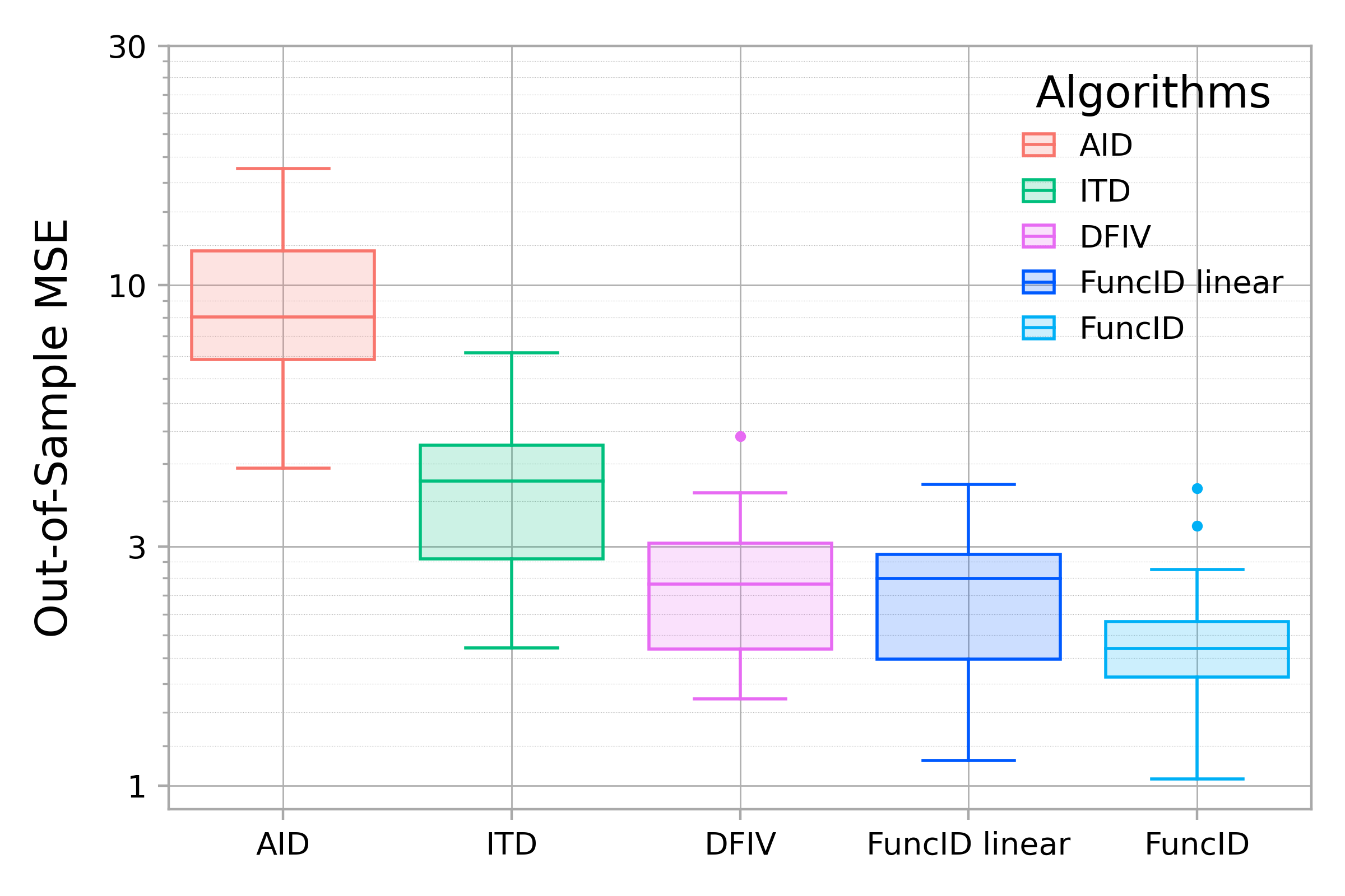
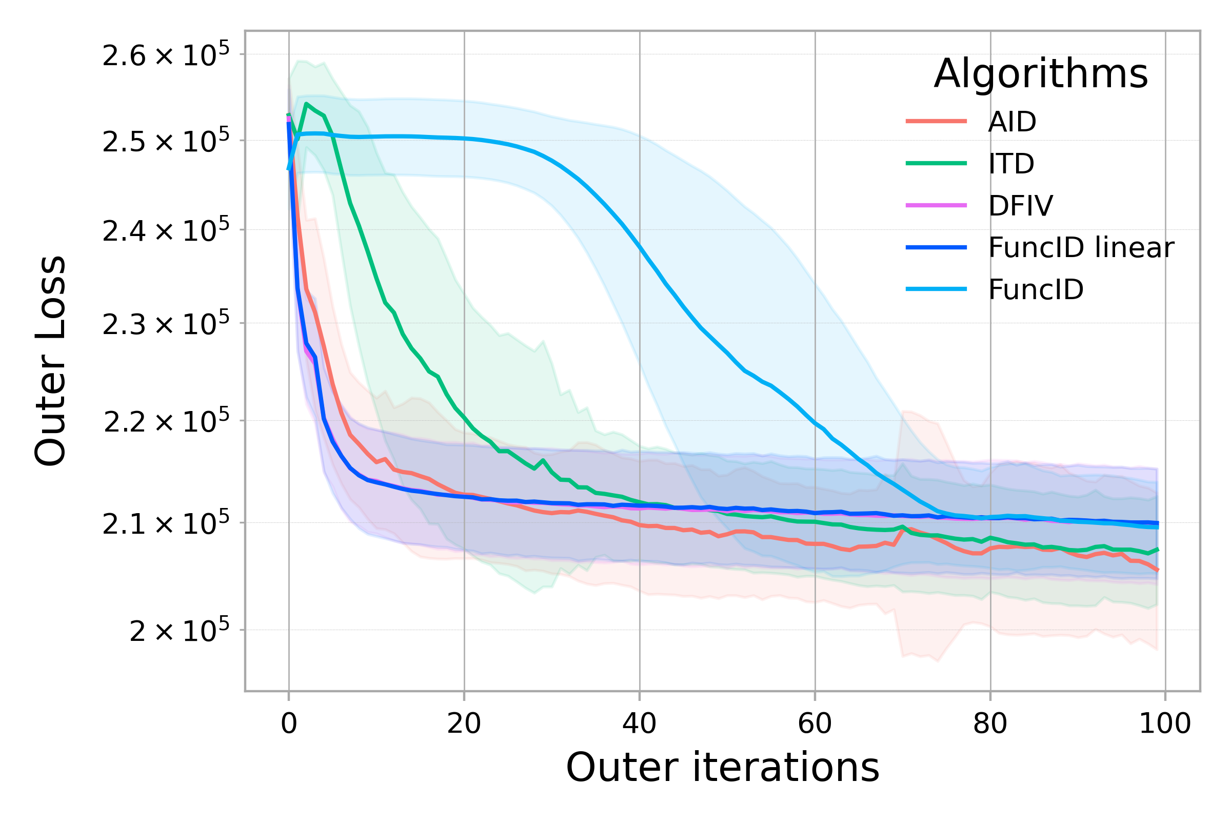
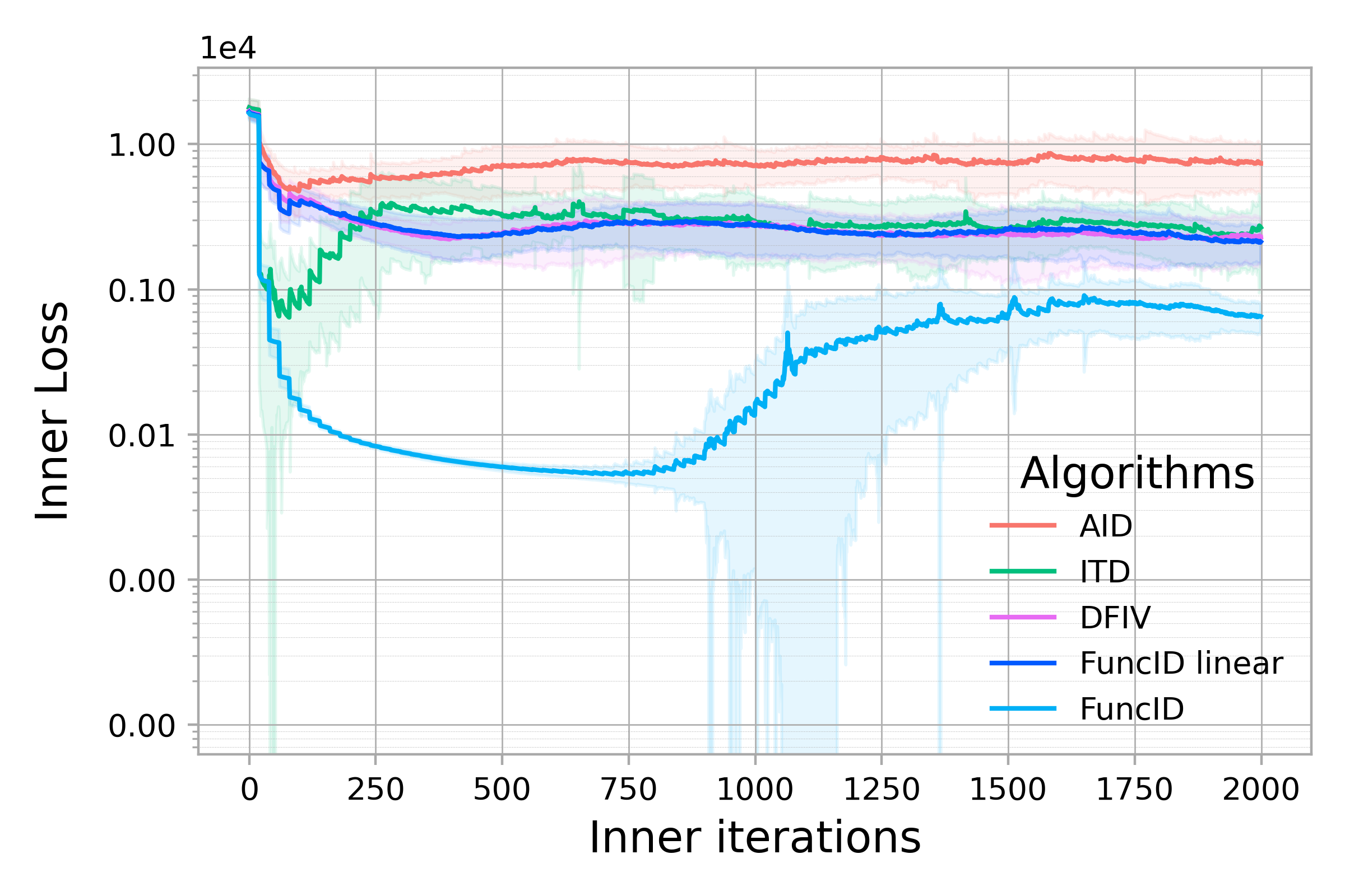
Figure 3: Performance metrics for Instrumental Variable (IV) regression. (Left) test loss, (Middle) outer loss vs training iterations, (Right) inner loss vs training iterations. All results are averaged over 20 runs with 5000 training samples and 588 test samples. The bold line in training loss plots is the mean loss, the shaded area corresponds to standard deviation.

Results.

Figure 3 compares the structural models learned by the different methods using 5K training samples (see Figure 5 in Section E.3 for similar results using 10K samples). Figure 3 (left) shows the out-of-sample mean squared error of the learned structural models compared to ground truth outcomes (uncontaminated by the confounding noise $\epsilon$), while Figure 3 (middle and right) show the evolution of the outer and inner objectives as a function of iterations. Our method FuncID improves over the reported state-of-the-art performance of DFIV [Xu et al., 2021a] on the dsprites dataset in terms of out-of-sample error. On the other hand, AID is the worst performing method followed by ITD. This suggests that, on the contrary to FuncID, the parametric point of view adopted by AID and ITD does not take full advantage of the functional structure in Equations 11 and 12. All methods recover similar outer losses (middle Figure 3), while inner solutions differ (right Figure 3) with FuncID obtaining the lowest value. This suggests that a smaller value for the outer loss in a 2SLS problems does not always imply a better generalization performance on the evaluation set, since imposing the correct inner-level constraint is also important. Overall, FuncID solves the considered 2SLS problem efficiently by effectively taking into account its functional structure, leading to better generalization.

5.2 Model-based reinforcement learning

Model-based reinforcement learning (RL) has proven to be a learning paradigm that naturally gives rise to bilevel optimization, since several components of an RL agent need to be learned using different objectives. Recently, Nikishin et al. [2022] showed that casting model-based reinforcement learning as a bilevel problem can result in better tolerance to model-misspecification. Our experiments show that the functional bilevel framework yields improved results even when the model is well-specified, suggesting a broader use of the bilevel formulation for model-based RL.

Problem formulation.

In model-based RL, the Markov Decision Process (MDP) is approximated by a probabilistic model $q_{\omega}$ with parameters $\omega$ that can predict the next state $s_{\omega}(x)$ and reward $r_{\omega}(x)$, given a pair $x:=(s,a)$ where $s$ is the current environment state and $a$ is the action of an agent. A second model $h$ can be used to approximate the action-value function $h(x)$ that computes the expected cumulative reward given the current state-action pair. Traditionally, the action-value function is learned using the current MDP model, while the latter is learned independently from the action-value function using Maximum Likelihood Estimation (MLE) [Sutton, 1991].

In the bilevel formulation of model-based RL proposed in Nikishin et al. [2022], the inner-level problem is to learn the optimal action-value function $h_{\omega}^{\star}$ using the current MDP model $q_{\omega}$ and minimizing the Bellman error relatively to the MDP model. The inner-level objective can be written as an expectation of a point-wise loss $f$ with samples $(x,r^{\prime},s^{\prime})\sim\mathbb{P}$, obtained from the interaction between the agent and its environment:

$$h_{\omega}^{\star}=\arg\min_{h\in\mathcal{H}}\mathbb{E}_{\mathbb{P}}\left[f(h(x),r_{\omega}(x),s_{\omega}(x))\right].$$ (13)

Here the future state and reward $(r^{\prime},s^{\prime})$ are replaced by the MDP model predictions $r_{\omega}(x)$ and $s_{\omega}(x)$. In practice, samples from $\mathbb{P}$ are obtained using a replay buffer. The buffer accumulates data over several episodes of interactions with the environment, and can therefore be considered independent of the agent’s policy. The point-wise loss function $f$ represents the error between the action-value function prediction and the expected cumulative reward given the current state-action pair:

$$f(v,r^{\prime},s^{\prime}):=\frac{1}{2}\left\lVert v-r^{\prime}-\gamma\log\sum_{a^{\prime}}e^{\bar{h}(s^{\prime},a^{\prime})}\right\rVert^{2},$$

with $\bar{h}$ a lagged version of $h$ (exponentially averaged network) and $\gamma$ a discount factor. The MDP model is learned implicitly using the optimal function $h_{\omega}^{\star}$, by minimizing the Bellman error relatively to the true MDP w.r.t. $\omega$:

$$\min_{\omega\in\Omega}\ \mathbb{E}_{\mathbb{P}}\left[f(h_{\omega}^{\star}(x),r^{\prime},s^{\prime})\right].$$ (14)

Equations 14 and 13 define a bilevel problem as in Equation 7, where $\mathbb{Q}=\mathbb{P}$, $y=(r^{\prime},s^{\prime})$, and the point-wise losses $\ell_{in}$ and $\ell_{out}$ are given by: $\ell_{in}\left(\omega,v,x,y\right)=f\left(v,r_{\omega}(x),s_{\omega}(x)\right)$ and $\ell_{out}\left(\omega,v,x,y\right)=f\left(v,r^{\prime},s^{\prime}\right)$. Therefore, we can directly apply Algorithm 1 to learn both the MDP model $q_{\omega}$ and the optimal action-value function $h_{\omega}^{\star}$.

Experimental setup.

We apply our FuncID method to the CartPole learning control problem, a well-known benchmark task in reinforcement learning [Brockman et al., 2016, Nagendra et al., 2017]. In this problem, a cart is attached to a pole via a joint, and the maximum reward is achieved when the agent can balance the pole upright by moving the cart horizontally. Following Nikishin et al. [2022], we use a model-based approach and consider two choices for the MDP model: a well-specified network, that can accurately represent the ground truth MDP, and a misspecified one, with a limited number of hidden layer units. Less hidden layer units limits the model’s capacity to represent the ground truth MDP. Using the bilevel formulation in Equations 13 and 14, we compare our method, FuncID, with the Optimal Model Design (OMD) algorithm from Nikishin et al. [2022], a variant of AID. Additionally, we compare against a commonly used single-level formulation of model-based RL that uses MLE to learn the MDP model independently from the action-value function [Sutton, 1991]. For the adjoint function unsed in funcID, we exploit the structure of the adjoint objective to provide a simple closed-form expression as further discussed in Section F.1. We then closely follow the experimental setup in Nikishin et al. [2022] and provide full details and hyperparameters in Section F.2.

Results.

Figure 4: Average reward on an evaluation environment vs. training iterations on the CartPole task. (Left) Well-specified model. (Right) Misspecified model with 3 hidden units. Both plots show mean reward over 10 runs where the shaded region is the 95% confidence interval.

Figure 4 shows the evolution of the reward during training for FuncID, OMD and MLE in both well-specified and misspecified settings. FuncID is consistently amongst the best performing methods in both settings. In the well-specified setting, where OMD under-performs MLE and attains only a reward of $4$, FuncID attains the maximum possible reward of $5$ performing as well as MLE (left Figure 4). In the miss-specified setting, FuncID demonstrates a performance comparable to OMD and significantly better than MLE (right Figure 4). Additionally, we find that FuncID tends to converge faster than MLE (see Figure 6 in Section F.3) and results in consistently better prediction error than OMD (see Figure 7 in Section F.3). These results are consistent with those in Nikishin et al. [2022], and support the hypothesis that MLE might prioritize reducing errors in predictions in the misspecified setting, leading to the model fitting irrelevant features in the data, and negatively impacting the performance of the agent. On the other hand, OMD and FuncID explicitly target maximizing the expected returns by learning a model that is more effective for decision-making, especially in the presence of MDP model misspecification. Our results further show that the bilevel formulation can also be beneficial in the well-specified setting when using algorithm such as FuncID, that exploit the functional structure of the problem.

Acknowledgments

This work was supported by the ERC grant number 101087696 (APHELAIA project) and by ANR 3IA MIAI@Grenoble Alpes (ANR-19-P3IA-0003) and the ANR project BONSAI (grant ANR-23-CE23-0012-01).

Appendix A Examples of FBO formulations

The functional bilevel setting covers several bilevel problems encountered in practice where the objectives depend only on the model predictions regardless of its parameterization. We discuss a few examples below.

Auxiliary task learning.

As in Equation 1, consider a main prediction task with features $x$ and labels $y$, equipped with a loss function $f(y,h(x))$. The goal of auxiliary task learning is to learn how a set of auxiliary tasks represented by a vector $f_{aux}(y,h(x))$ could help solve the main task. This problem is formulated by Navon et al. [2021] as a bilevel problem, which can be written as (FBO) with

$$L_{out}(\omega,h)={\mathbb{E}}_{(y,x)\sim{\mathcal{D}}_{val}}\left[f(y,h(x))\right],$$

where the loss is evaluated over a validation dataset $\mathcal{D}_{val}$, and

$$L_{in}(\omega,h)={\mathbb{E}}_{(y,x)\sim{\mathcal{D}}_{train}}\left[f(y,h(x))+g_{\omega}(f_{aux}(y,h(x)))\right],$$

where an independent training dataset $\mathcal{D}_{train}$ is used, and $g_{\omega}$ is a function that combines the auxiliary losses into a scalar value.

Task-driven metric learning.

Considering now a regression problem with features $x$ and labels $y$, the goal of task-driven metric learning formulated by Bansal et al. [2023] is to learn a metric parameterized by $\omega$ for the regression task such that the corresponding predictor $h_{\omega}^{\star}$ performs well on a downstream task $L_{task}$. This can be formulated as (FBO) with $L_{out}(\omega,h)=L_{task}(h)$ and

$$L_{in}(\omega,h)={\mathbb{E}}_{(y,x)}\left[\|y-h(x)\|_{A_{\omega}(x)}^{2}\right],$$

where $\|\cdot\|^{2}_{\omega}$ is the squared Mahalanobis norm with parameters $\omega$ and $A_{\omega}(x)$ is a data-dependent metric that allows emphasizing features that are more important for the downstream task.

Appendix B General functional implicit differentiation

B.1 Preliminary results

We recall the definition of Hadamard differentiability and provide in Proposition B.2 a general property for Hadamard differentiable maps that we will exploit to prove Theorem 3.1 in Section B.2.

Definition B.1.

Hadamard differentiability. Let $A$ and $B$ be two separable Banach spaces. A function $L:A\rightarrow B$ is said to be Hadamard differentiable [van der Vaart, 1991, Fang and Santos, 2018] if for any $a\in A$, there exist a continuous linear map $d_{a}L(a):A\rightarrow B$ so that for any sequence $(u_{n})_{n\geq 1}$ in $A$ converging to an element $u\in A$, and any real valued and non-vanishing sequence $(t_{n})_{n\geq 1}$ converging to $0$, it holds that:

$$\left\lVert\frac{1}{t_{n}}\left(L(a+t_{n}u_{n})-L(a)\right)-d_{a}L(a)u\right\rVert\xrightarrow[n\rightarrow+\infty]{}0.$$ (15)

Proposition B.2.

Let $A$ and $B$ be two separable Banach spaces. Let $L:A\rightarrow B$ be a Hadamard differentiable map with differential $d_{a}L$ at point $a$. Consider a bounded linear map defined over a euclidean space $\mathbb{R}^{n}$ of finite dimension $n$ and taking values in $A$, i.e $J:\mathbb{R}^{n}\rightarrow A$. Then, the following holds:

$$L(a+Ju)=L(a)+d_{a}L(a)Ju+o(\left\lVert u\right\rVert).$$

Proof.

Consider a sequence $(u_{k})_{k\geq 1}$ in $\mathbb{R}^{n}$ so that $u_{k}$ converges to $0$ with $\left\lVert u_{k}\right\rVert>0$ for all $k\geq 1$ and define the first order error $E_{k}$ as follows:

$$E_{k}=\frac{1}{\left\lVert u_{k}\right\rVert}\left\lVert L(a+Ju_{k})-L(a)-d_{a}L(a)u_{k}\right\rVert.$$

The goal is to show that $E_{k}$ converges to $0$. We can write $u_{k}$ as $u_{k}=t_{k}\tilde{u}_{k}$ with $t_{k}=\left\lVert u_{k}\right\rVert$ and $\left\lVert\tilde{u}_{k}\right\rVert=1$, so that:

$$E_{k}=\left\lVert\frac{1}{\left\lVert t_{k}\right\rVert}\left(L(a+t_{k}J\tilde{u}_{k})-L(a)\right)-d_{a}L(a)\tilde{u}_{k}\right\rVert.$$

If $E_{k}$ were unbounded, then, by contradiction, there must exist a subsequence $(E_{\phi(k)})_{k\geq 1}$ converging to $+\infty$, with $\phi(k)$ increasing and $\phi(k)\rightarrow+\infty$. Moreover, since $\tilde{u}_{k}$ is bounded, one can further choose the subsequence $E_{\phi(k)}$ so that $\tilde{u}_{\phi(k)}$ converges to some element $\tilde{u}$. We can use the following upper-bound:

$$E_{k}\leq\underbrace{\left\lVert\frac{1}{\left\lVert t_{k}\right\rVert}\left(L(a+t_{k}J\tilde{u}_{k})-L(a)\right)-d_{a}L(a)\tilde{u}\right\rVert}_{\tilde{E}_{k}}+\left\lVert d_{a}L(a)\right\rVert\left\lVert\tilde{u}_{k}-\tilde{u}\right\rVert,$$ (16)

where we used that $d_{a}L(a)$ is bounded. Since $L$ is Hadamard differentiable, $\tilde{E}_{\phi(k)}$ converges to $0$. Moreover, $\left\lVert\tilde{u}_{\phi(k)}{-}\tilde{u}\right\rVert$ also converges to $0$. Hence, $E_{\phi(k)}$ converges to $0$ which contradicts $E_{\phi(k)}{\rightarrow}{+}\infty$. Therefore, $E_{k}$ is bounded.

Consider now any convergent subsequence of $(E_{k})_{k\geq 1}$. Then, it can be written as $(E_{\phi(k)})_{k\geq 1}$ with $\phi(k)$ increasing and $\phi(k)\rightarrow+\infty$. We then have $E_{\phi(k)}\rightarrow e<+\infty$ by construction. Since $\tilde{u}_{k}$ is bounded, one can further choose the subsequence $E_{\phi(k)}$ so that $\tilde{u}_{\phi(k)}$ converges to some element $\tilde{u}$. Using again Equation 16 and the fact that $L$ is Hadamard differentiable, we deduce that $\tilde{E}_{\phi(k)}$ must converge to $0$, and by definition of $\tilde{u}_{\phi(k)}$, that $\left\lVert\tilde{u}_{\phi(k)}-\tilde{u}\right\rVert$ converges to $0$. Therefore, it follows that $E_{\phi(k)}\rightarrow 0$, so that $e=0$. We then have shown that $(E_{k})_{k\geq 1}$ is a bounded sequence and every subsequence of it converges to $0$. Therefore, $E_{k}$ must converge to $0$, which concludes the proof. ∎

B.2 Proof of the Functional implicit differentiation theorem

Proof of Theorem 3.1.

The proof strategy consists in establishing the existence and uniqueness of the solution map $\omega\mapsto h_{\omega}^{\star}$, deriving a candidate Jacobian for it, then proving that $\omega\mapsto h_{\omega}^{\star}$ is differentiable.

Existence and uniqueness of a solution map $\omega\mapsto h_{\omega}^{\star}$. Let $\omega$ in $\Omega$ be fixed. The map $h\mapsto L_{in}(\omega,h)$ is lower semi-continuous since it is Fréchet differentiable by assumption. It is also strongly convex. Therefore, it admits a unique minimier $h_{\omega}^{\star}$ [Bauschke and Combettes, 2011, Corollary 11.17]. We then conclude that the map $\omega\mapsto h_{\omega}^{\star}$ is well-defined on $\Omega$.

Strong convexity inequalities. We provide two inequalities that will be used for proving differentiability of the map $\omega\mapsto h_{\omega}^{\star}$. The map $h\mapsto L_{in}(\omega,h)$ is Fréchet differentiable on $\mathcal{H}$ and $\mu$-strongly convex (with $\mu$ positive by assumption). Hence, for all $h_{1},h_{2}$ in $\mathcal{H}$ the following quadratic lower-bound holds:

$$L_{in}(\omega,h_{2})\geq L_{in}(\omega,h_{1})+\langle\partial_{h}L_{in}(\omega,h_{1}),(h_{2}-h_{1})\rangle_{\mathcal{H}}+\frac{\mu}{2}\left\lVert h_{2}-h_{1}\right\rVert_{\mathcal{H}}^{2}.$$ (17)

From the inequality above, we can also deduce that $h\mapsto\partial_{h}L_{in}(\omega,h)$ is a $\mu$-strongly monotone operator:

$$\langle\partial_{h}L_{in}(\omega,h_{1})-\partial_{h}L_{in}(\omega,h_{2}),h_{1}-h_{2}\rangle_{\mathcal{H}}\geq\mu\left\lVert h_{1}-h_{2}\right\rVert_{\mathcal{H}}^{2}.$$ (18)

Finally, note that, since $h\mapsto L_{in}(\omega,h)$ is Fréchet differentiable, its gradient must vanish at the optimum $h_{\omega}^{\star}$, i.e :

$$\partial_{h}L_{in}(\omega,h_{\omega}^{\star})=0.$$ (19)

Candidate Jacobian for $\omega\mapsto h_{\omega}^{\star}$. Let $\omega$ be in $\Omega$. Using Equation 18 with $h_{1}=h+tv$ and $h_{2}=h$ for some $h,v\in\mathcal{H}$, and a non-zeros real number $t$ we get:

$$\frac{1}{t}\langle\partial_{h}L_{in}(\omega,h+tv)-\partial_{h}L_{in}(\omega,h),v\rangle_{\mathcal{H}}\geq\mu\left\lVert v\right\rVert^{2}.$$ (20)

By assumption, $h\mapsto\partial_{h}L_{in}(\omega,h)$ is Hadamard differentiable and, a fortiori, directionally differentiable. Thus, by taking the limit when $t\rightarrow 0$, it follows that:

$$\langle\partial_{h}^{2}L_{in}(\omega,h)v,v\rangle_{\mathcal{H}}\geq\mu\left\lVert v\right\rVert^{2}.$$ (21)

Hence, $\partial_{h}^{2}L_{in}(\omega,h):\mathcal{H}\rightarrow\mathcal{H}$ defines a coercive quadratic form. By definition of Hadamard differentiability, it is also bounded. Therefore, it follows from Lax-Milgram’s theorem [Debnath and Mikusinski, 2005, Theorem 4.3.16], that $\partial_{h}^{2}L_{in}(\omega,h)$ is invertible with a bounded inverse. Moreover, recalling that $B_{\omega}=\partial_{\omega,h}L_{in}(\omega,h_{\omega}^{\star})$ is a bounded operator, its adjoint $(B_{\omega})^{\star}$ is also a bounded operator from $\Omega$ to $\mathcal{H}$. Therefore, we can define $J=-C_{\omega}^{-1}(B_{\omega})^{\star}$ which is a bounded linear map from $\Omega$ to $\mathcal{H}$ and will be our candidate Jacobian.

Differentiability of $\omega\mapsto h_{\omega}^{\star}$. By the strong convexity assumption (locally in $\omega$), there exists an open ball $\mathcal{B}$ centered at the origin $0$ that is small enough so that we can ensure the existence of $\mu>0$ for which $h\mapsto L_{in}(\omega+\epsilon,h)$ is $\mu$-strongly convex for all $\epsilon\in\mathcal{B}$. For a given $\epsilon\in\mathcal{B}$, we use the $\mu$-strong monotonicity of $h\mapsto\partial_{h}L_{in}(\omega+\epsilon,h)$ (18) at points $h_{\omega}^{\star}+J\epsilon$ and $h_{\omega+\epsilon}^{\star}$ to get:

$$\mu\left\lVert h_{\omega+\epsilon}^{\star}-h_{\omega}^{\star}-J\epsilon\right\rVert^{2} \leq\langle\left(\partial_{h}L_{in}\left(\omega+\epsilon,h_{\omega+\epsilon}^{\star}\right)-\partial_{h}L_{in}\left(\omega+\epsilon,h_{\omega}^{\star}+J\epsilon\right)\right),\left(h_{\omega+\epsilon}^{\star}-h_{\omega}^{\star}-J\epsilon\right)\rangle_{\mathcal{H}}$$

$$=\langle-\partial_{h}L_{in}\left(\omega+\epsilon,h_{\omega}^{\star}+J\epsilon\right),\left(h_{\omega+\epsilon}^{\star}-h_{\omega}^{\star}-J\epsilon\right)\rangle_{\mathcal{H}}$$

$$\leq\left\lVert\partial_{h}L_{in}\left(\omega+\epsilon,h_{\omega}^{\star}+J\epsilon\right)\right\rVert_{\mathcal{H}}\left\lVert h_{\omega+\epsilon}^{\star}-h_{\omega}^{\star}-J\epsilon\right\rVert_{\mathcal{H}},$$

where the second line follows from optimality of $h^{\star}_{\omega+\epsilon}$ (Equation 19), and the last line uses Cauchy-Schwarz’s inequality. The above inequality allows us to deduce that:

$$\left\lVert h_{\omega+\epsilon}^{\star}-h_{\omega}^{\star}-J\epsilon\right\rVert\leq\frac{1}{\mu}\left\lVert\partial_{h}L_{in}\left(\omega+\epsilon,h_{\omega}^{\star}+J\epsilon\right)\right\rVert_{\mathcal{H}}.$$ (22)

Moreover, since $\partial_{h}L_{in}$ is Hadamard differentiable, by Proposition B.2 it follows that:

$$\partial_{h}L_{in}\left(\omega+\epsilon,h_{\omega}^{\star}+J\epsilon\right)= \underbrace{\partial_{h}L_{in}\left(\omega,h_{\omega}^{\star}\right)}_{=0}+d_{(\omega,h)}\partial_{h}L_{in}(\omega,h_{\omega}^{\star})(\epsilon,J\epsilon)+o(\left\lVert\epsilon\right\rVert),$$ (23)

where the first term vanishes thanks to Equation 19, since $h_{\omega}^{\star}$ is a minimizer of $h\mapsto L_{in}(\omega,h)$. Additionally, note that the differential $d_{(\omega,h)}\partial_{h}L_{in}(\omega,h):\Omega\times\mathcal{H}\rightarrow\mathcal{H}$ acts on elements $(\epsilon,g)\in\Omega\times\mathcal{H}$ as follows:

$$d_{(\omega,h)}\partial_{h}L_{in}(\omega,h)(\epsilon,g)=\partial_{h}^{2}L_{in}(\omega,h)g+\left(\partial_{\omega,h}L_{in}(\omega,h)\right)^{\star}\epsilon,$$ (24)

where $\partial_{h}^{2}L_{in}(\omega,h):\mathcal{H}\rightarrow\mathcal{H}$ and $\partial_{\omega,h}L_{in}(\omega,h):\mathcal{H}\rightarrow\Omega$ are bounded operators and $\left(\partial_{\omega,h}L_{in}(\omega,h)\right)^{\star}$ denotes the adjoint of $\partial_{\omega,h}L_{in}(\omega,h)$. By definition of $J$, and using Equation 24, it follows that:

$$d_{(\omega,h)}\partial_{h}L_{in}(\omega,h)(\epsilon,J\epsilon) =C_{\omega}J\epsilon+B_{\omega}\epsilon=0.$$

Therefore, combining Equation 23 with the above equality yields:

$$\partial_{h}L_{in}\left(\omega+\epsilon,h_{\omega}^{\star}+J\epsilon\right)=o(\left\lVert\epsilon\right\rVert).$$ (25)

Finally, combining Equation 22 with the above equality directly shows that $\left\lVert h_{\omega+\epsilon}^{\star}-h_{\omega}^{\star}-J\epsilon\right\rVert\leq\frac{1}{\mu}o(\left\lVert\epsilon\right\rVert)$. We have shown that $\omega\mapsto h_{\omega}^{\star}$ is differentiable with a Jacobian map $\partial_{\omega}h_{\omega}^{\star}$ given by $J^{\star}=-B_{\omega}C_{\omega}^{-1}$. ∎

B.3 Proof of the functional adjoint sensitivity in Proposition 3.2

Proof of Proposition 3.2.

We use the assumptions and definitions from Proposition 3.2 and express the gradient $\nabla\mathcal{F}(\omega)$ using the chain rule:

$$\nabla\mathcal{F}(\omega)=\partial_{\omega}L_{out}(\omega,h^{\star}_{\omega})+\left[\partial_{\omega}h^{\star}_{\omega}\right]\partial_{h}L_{out}(\omega,h^{\star}_{\omega}).$$

The Jacobian $\partial_{\omega}h^{\star}_{\omega}$ is the solution of a linear system obtained by applying Theorem 3.1 :

$$\partial_{\omega}h^{\star}_{\omega}=-B_{\omega}C_{\omega}^{-1}.$$

We note $g_{\omega}=\partial_{\omega}L_{out}(\omega,h^{\star}_{\omega})$ and $d_{\omega}=\partial_{h}L_{out}(\omega,h^{\star}_{\omega})$. It follows that the gradient $\nabla\mathcal{F}(\omega)$ can be expressed as:

$$\nabla\mathcal{F}(\omega)=g_{\omega}+\left[\partial_{\omega}h^{\star}_{\omega}\right]d_{\omega}=g_{\omega}+{B}_{\omega}a_{\omega}^{\star}$$

$$a_{\omega}^{\star}:=-C_{\omega}^{-1}d_{\omega}.$$

In other words, the implicit gradient $\nabla\mathcal{F}(\omega)$ can be expressed using the adjoint function $a_{\omega}^{\star}$, which is an element of $\mathcal{H}$ and can be defined as the solution of the following functional regression problem:

$$a_{\omega}^{\star}=\arg\min_{a\in\mathcal{H}}L_{adj}(\omega,a):=\tfrac{1}{2}\ \langle a,C_{\omega}a\rangle_{\mathcal{H}}+\langle a,d_{\omega}\rangle_{\mathcal{H}}.$$

∎

Appendix C Connection with parametric implicit differentiation

To establish a connection with parametric implicit differentiation, let us consider $\tau:\Theta\mapsto\mathcal{H}$ to be a map from a finite dimensional set of parameters $\Theta$ to the functional Hilbert space $\mathcal{H}$ and define a parametric version of the outer and inner objectives in Equation FBO restricted to functions in $\mathcal{H}_{\Theta}:=\left\{\tau(\theta)~{}\middle|~{}\theta\in\Theta\right\}$:

$$G_{out}(\omega,\theta):=L_{out}\left(\omega,\tau(\theta)\right)\qquad G_{in}(\omega,\theta):=L_{in}\left(\omega,\tau(\theta)\right).$$ (26)

The map $\tau$ can typically be a neural network parameterization and allows to obtain a “more tractable” approximation to the abstract solution $h_{\omega}^{\star}$ in $\mathcal{H}$ where the function space $\mathcal{H}$ is often too large to perform optimization. This is typically the case when $\mathcal{H}$ is an $L_{2}$-space of functions as we discuss in more details in Section 4. When $\mathcal{H}$ is a Reproducing Kernel Hilbert Space (RKHS), $\tau$ may also correspond to the Nyström approximation [Williams and Seeger, 2000], which performs the optimization on a finite-dimensional subspace of an RKHS spanned by a few data points.

The corresponding parametric version of the problem (FBO) is then formally defined as:

$$\begin{split}\min_{\omega\in\Omega}\ G_{tot}(\omega)&:=G_{out}(\omega,\theta_{\omega}^{\star})\\ \text{s.t. }\theta^{\star}_{\omega}&\in\operatorname*{arg\,min}_{\theta\in\Theta}\ G_{in}(\omega,\theta).\end{split}$$ (PBO)

The resulting bilevel problem in Equation PBO often arises in machine learning but is generally ambiguously defined without further assumptions on the map $\tau$ as the inner-level problem might admit multiple solutions [Arbel and Mairal, 2022b]. Under the assumption that $\tau$ is twice continuously differentiable and the rather strong assumption that the parametric Hessian $\partial_{\theta}^{2}G_{in}(\omega,\theta_{\omega}^{\star})$ is invertible for a given $\omega$, the expression for the total gradient $\nabla_{\omega}G_{tot}(\omega)$ follows by direct application of the parametric implicit function theorem [Pedregosa, 2016]:

$$\begin{split}\nabla_{\omega}G_{tot}(\omega)&=\partial_{\omega}G_{out}(\omega,\theta_{\omega}^{\star})+\partial_{\omega,\theta}G_{in}(\omega,\theta_{\omega}^{\star})u_{\omega}^{\star}\\ u_{\omega}^{\star}&=-\partial_{\theta}^{2}G_{in}(\omega,\theta_{\omega}^{\star})^{-1}\partial_{\theta}G_{out}(\omega,\theta_{\omega}^{\star}),\end{split}$$ (27)

where $u_{\omega}^{\star}$ is the adjoint vector in ${\Theta}$. Without further assumptions, the expression of the gradient in Equation 27 is generally different from the one obtained in Proposition 3.2 using the functional point of view. Nevertheless, a precise connection between the functional and parametric implicit gradients can be obtained under expressiveness assumptions on the parameterization $\tau$, as discussed in the next two propositions.

Proposition C.1.

Under the same assumptions as in Proposition 3.2 and assuming that $\tau$ is twice continuously differentiable, the following expression holds for any $(\omega,\theta)\in\Omega\times\Theta$:

$$\partial_{\theta}^{2}G_{in}(\omega,\theta):=\partial_{\theta}\tau(\theta)\partial_{h}^{2}L_{in}(\omega,\tau(\theta))\partial_{\theta}\tau(\theta)^{\top}+\partial_{\theta}^{2}\tau(\theta)\left[\partial_{h}L_{in}(\omega,\tau(\theta))\right],$$ (28)

where $\partial_{\theta}^{2}\tau(\theta)$ is a linear operator measuring the distortion induced by the parameterization and acts on functions in $\mathcal{H}$ by mapping them to a matrix $p\times p$ where $p$ is the dimension of the parameter space $\Theta$. If, in addition, $\tau$ is expressive enough so that $\tau(\theta^{\star}_{\omega})=h_{\omega}^{\star}$, then the above expression simplifies to:

$$\partial_{\theta}^{2}G_{in}(\omega,\theta^{\star}_{\omega}):= \partial_{\theta}\tau(\theta^{\star}_{\omega})C_{\omega}\partial_{\theta}\tau(\theta_{\omega}^{\star})^{\top}.$$ (29)

Proposition C.1 follows by direct application of the chain rule, noting that the distortion term on the right of (28) vanishes when $\theta=\theta_{\omega}^{\star}$ since $\partial_{h}L_{in}(\omega,\tau(\theta_{\omega}^{\star}))=\partial_{h}L_{in}(\omega,h_{\omega}^{\star})=0$ by optimality of $h_{\omega}^{\star}$. A consequence is that, for an optimal parameter $\theta^{\star}_{\omega}$, the parametric Hessian is necessarily symmetric positive semi-definite. However, for an arbitrary parameter $\theta$, the distortion does not vanish in general, making the Hessian possibly non-positive. This can result in numerical instability when using algorithms such as AID for which an adjoint vector is obtained by solving a quadratic problem defined by the Hessian matrix $\partial_{\theta}^{2}G_{in}$ evaluated on approximate minimizers of the inner-level problem. Moreover, if the model admits multiple solutions $\theta^{\star}_{\omega}$, the Hessian is likely to be degenerate making the implicit function theorem inapplicable and the bilevel problem in Equation PBO ambiguously defined. On the other hand, the functional implicit differentiation requires finding an adjoint function $a_{\omega}^{\star}$ by solving a positive definite quadratic problem in $\mathcal{H}$ which is always guaranteed to have a solution even when the inner-level prediction function is only approximately optimal.

Proposition C.2.

Assuming that $\tau$ is twice continuously differentiable and that for a fixed $\omega\in\Omega$ we have $\tau(\theta_{\omega}^{\star})=h_{\omega}^{\star}$, and $J_{\omega}:=\partial_{\theta}\tau(\theta_{\omega}^{\star})$ has a full rank, then, under the same assumptions as in Proposition 3.2, $\nabla_{\omega}G_{tot}(\omega)$ is given by:

$$\nabla_{\omega}G_{tot}(\omega)=g_{\omega}+B_{\omega}P_{\omega}a_{\omega}^{\star},$$ (30)

where $P_{\omega}:\mathcal{H}\to\mathcal{H}$ is a projection operator of rank $\dim(\Theta)$. If, in addition, the equality $\tau(\theta_{\omega^{\prime}}^{\star})=h_{\omega^{\prime}}^{\star}$ holds for all $\omega^{\prime}$ in a neighborhood of $\omega$, then $\nabla_{\omega}G_{tot}(\omega):=\nabla\mathcal{F}(\omega)=g_{\omega}+B_{\omega}a_{\omega}^{\star}$.

Proposition C.2, which is proven below, shows that, even when the parametric family is expressive enough to recover the optimal prediction function $h_{\omega}^{\star}$ at a single value $\omega$, the expression of the total gradient in Equation 30 using parametric implicit differentiation might generally differ from the one obtained using its functional counterpart. Indeed the projector $P_{\omega}$, which has a rank equal to $\dim(\Theta)$, biases the adjoint function by projecting it into a finite dimensional space before applying the cross derivative operator. Only under a much stronger assumption on $\tau$, requiring it to recover the optimal prediction function $h_{\omega}^{\star}$ in a neighborhood of the outer-level variable $\omega$, both parametric and functional implicit differentiation recover the same expression for the total gradient. In this case, the projector operator aligns with the cross-derivative operator so that $B_{\omega}P_{\omega}=B_{\omega}$. Finally, note that the expressiveness assumptions on $\tau$ made in Propositions C.1 and C.2 are only used here to discuss the connection with the parametric implicit gradient and are not required by the method we introduce in Section 4.

Proof of Proposition C.2.

Here we want to show the connection between the parametric gradient of the outer variable $\nabla_{\omega}G_{tot}(\omega)$ usually used in approximate differentiation methods and the functional gradient of the outer variable $\nabla\mathcal{F}(\omega)$ derived from the functional bilevel problem definition in Equation FBO. Recall the definition of the parametric inner objective $G_{in}(\omega,\theta):=L_{in}\left(\omega,\tau(\theta)\right)$. According to Proposition C.1, we have the following relation

$$\partial_{\theta}^{2}G_{in}(\omega,\theta^{\star}_{\omega}):= J_{\omega}C_{\omega}J_{\omega}^{\top}~{}~{}~{}\text{with}~{}~{}~{}J_{\omega}:=\partial_{\theta}\tau(\theta_{\omega}^{\star}).$$

By assumption, $J_{\omega}$ has a full rank which matches the dimension of the parameter space $\Theta$. Recall from the assumptions of Theorem 3.1 that the Hessian operator $C_{\omega}$ is positive definite by the strong convexity of the inner-objective $L_{in}$ in the second argument. We deduce that $\partial_{\theta}^{2}G_{in}(\omega,\theta^{\star}_{\omega})$ must be invertible, since, by construction, the dimension of $\Theta$ is smaller than that of the Hilbert space $\mathcal{H}$ which has possibly infinite dimension. Recall from Theorem 3.1, $B_{\omega}:=\partial_{\omega,h}L_{in}(\omega,h^{\star}_{\omega})$ and the assumption that $\tau(\theta_{\omega}^{\star})=h_{\omega}^{\star}$. We apply the parametric implicit function theorem to get the following expression of the Jacobian $\partial_{\omega}\theta^{\star}_{\omega}$:

$$\partial_{\omega}\theta^{\star}_{\omega}:=-B_{\omega}J_{\omega}^{\top}\left(J_{\omega}C_{\omega}J_{\omega}^{\top}\right)^{-1}.$$

Hence, differentiating the total objective $G_{tot}(\omega):=G_{out}(\omega,\theta_{\omega}^{\star})=L_{out}\left(\omega,\tau(\theta_{\omega}^{\star})\right)$ and applying the chain rule directly results in the following expression:

$$\nabla_{\omega}G_{tot}(\omega)=g_{\omega}-B_{\omega}J_{\omega}^{\top}\left(J_{\omega}C_{\omega}J_{\omega}^{\top}\right)^{-1}J_{\omega}d_{\omega},$$ (31)

with previously defined $g_{\omega}:=\partial_{\omega}L_{out}(\omega,h^{\star}_{\omega})$ and $d_{\omega}:=\partial_{h}L_{out}\left(\omega,h_{\omega}^{\star}\right)$.

We now introduce the operator $P_{\omega}:=J_{\omega}^{\top}\left(J_{\omega}C_{\omega}J_{\omega}^{\top}\right)^{-1}J_{\omega}C_{\omega}$. The operator $P_{\omega}$ is a projector as it satisfies $P_{\omega}^{2}=P_{\omega}$. Hence, using the fact that the Hessian operator is invertible, and recalling that the adjoint function is given by $a_{\omega}^{\star}=-C_{\omega}^{-1}d_{\omega}$, we directly get form Equation 31 that:

$$\nabla_{\omega}G_{tot}(\omega):=g_{\omega}+B_{\omega}P_{\omega}a_{\omega}^{\star}.$$

If we further assume that $\tau(\theta_{\omega^{\prime}}^{\star})=h_{\omega^{\prime}}^{\star}$ holds for all $\omega^{\prime}$ in a neighborhood of $\omega$, then differentiating with respect to $\omega$ results in the following identity:

$$\partial_{\omega}\theta_{\omega}^{\star}J_{\omega}=\partial_{\omega}h_{\omega}^{\star}.$$

Using the expression of $\partial_{\omega}h_{\omega}^{\star}$ from Equation 4, we have the following identity:

$$-\partial_{\omega}\theta_{\omega}^{\star}J_{\omega}C_{\omega}=B_{\omega}.$$

In other words, $B_{\omega}$ is of the form $B_{\omega}:=DJ_{\omega}C_{\omega}$ for some finite dimensional matrix $D$ of size $\dim(\Omega)\times\dim(\Theta)$. Recalling the expression of the total gradient, we can deduce the equality between parametric and functional gradients:

$$\nabla_{\omega}G_{tot}(\omega) =g_{\omega}-B_{\omega}J_{\omega}^{\top}\left(J_{\omega}C_{\omega}J_{\omega}^{\top}\right)^{-1}J_{\omega}d_{\omega}$$

$$=g_{\omega}-DJ_{\omega}C_{\omega}J_{\omega}^{\top}\left(J_{\omega}C_{\omega}J_{\omega}^{\top}\right)^{-1}J_{\omega}d_{\omega}$$

$$=g_{\omega}-DJ_{\omega}d_{\omega}$$

$$=g_{\omega}-DJ_{\omega}C_{\omega}C_{\omega}^{-1}d_{\omega}$$

$$=g_{\omega}+B_{\omega}a_{\omega}^{\star}=\nabla\mathcal{F}(\omega).$$

The first equality follows from the general expression of the total gradient $\nabla_{\omega}G_{tot}(\omega)$. In the second line we use the expression of $B_{\omega}$ which then allows to simplify the expression in the third line. Then, recalling that the Hessian operator $C_{\omega}$ is invertible, we get the fourth line. Finally, the result follows by using again the expression of $B_{\omega}$ and recalling the definition of the adjoint function $a_{\omega}^{\star}$. ∎

Appendix D Functional adjoint sensitivity result in $L_{2}$ spaces

In this section we provides full proofs of Proposition 3.3. We start by stating the assumptions needed on the point-wise losses in Section D.1, then provide some differentiation results in Section D.2 and conclude with the main proofs in Section D.3.

D.1 Assumptions

Assumptions on $\ell_{in}$.

1. For any $\omega\in\Omega$, there exists a positive constant $\mu$ and a neighborhood $B$ of $\omega$ for which $\ell_{in}$ is $\mu$-strongly convex in its second argument for all $(\omega^{\prime},x,y)\in B\times\mathcal{X}\times\mathcal{Y}$.

2. For any $\omega\in\Omega$, $\mathbb{E}_{\mathbb{P}}\left[\left\lvert\ell_{in}(\omega,0,x,y)\right\rvert+\left\lVert\partial_{v}\ell_{in}\left(\omega,0,x,y\right)\right\rVert^{2}\right]<+\infty$.

3. $v\mapsto\ell_{in}(\omega,v,x,y)$ is continuously differentiable for all $(\omega,x,y)\in\Omega\times\mathcal{X}\times\mathcal{Y}$.

4. For any fixed $\omega\in\Omega$, there exists a constant $L$ and a neighborhood $B$ of $\omega$ s.t. $v\mapsto\ell_{in}(\omega^{\prime},v,x,y)$ is $L$-smooth for all $\omega^{\prime},x,y\in B\times\mathcal{X}\times\mathcal{Y}$.

5. $(\omega,v)\mapsto\partial_{v}\ell_{in}(\omega,v,x,y)$ is continuously differentiable on $\Omega\times\mathcal{V}$ for all $x,y\in\mathcal{X}\times\mathcal{Y}$,

6. For any $\omega\in\Omega$, there exists a positive constant $C$ and a neighborhood $B$ of $\omega$ s.t. for all $(\omega^{\prime},x,y)\in B\times\mathcal{X}\times\mathcal{Y}$:

   $$\left\lVert\partial_{\omega,v}\ell_{in}\left(\omega^{\prime},0,x,y\right)\right\rVert\leq C\left(1+\left\lVert x\right\rVert+\left\lVert y\right\rVert\right).$$ (32)

7. For any $\omega\in\Omega$, there exists a positive constant $C$ and a neighborhood $B$ of $\omega$ s.t. for all $(\omega^{\prime},v_{1},v_{2},x,y)\in B\times\mathcal{V}\times\mathcal{V}\times\mathcal{X}\times\mathcal{Y}$ we have:

   $$\left\lVert\partial_{\omega,v}\ell_{in}\left(\omega^{\prime},v_{1},x,y\right)-\partial_{\omega,v}\ell_{in}\left(\omega^{\prime},v_{2},x,y\right)\right\rVert\leq C\left\lVert v_{1}-v_{2}\right\rVert.$$ (33)

Assumptions on $\ell_{out}$.

1. For any $\omega\in\Omega$, $\mathbb{E}_{\mathbb{Q}}\left[\left\lvert\ell_{out}(\omega,0,x,y)\right\rvert\right]<+\infty$.

2. $(\omega,v)\mapsto\ell_{out}(\omega,v,x,y)$ is jointly continuously differentiable on $\Omega\times\mathcal{V}$ for all $(x,y)\in\mathcal{X}\times\mathcal{Y}$.

3. For any $\omega\in\Omega$, there exits a neighborhood $B$ of $\omega$ and a positive constant $C$ s.t. for all $(\omega^{\prime},v,v^{\prime},x,y)\in B\times\mathcal{V}\times\mathcal{V}\times\mathcal{X}\times\mathcal{Y}$ we have:

   $$\left\lVert\partial_{\omega}\ell_{out}\left(\omega^{\prime},v,x,y\right)-\partial_{\omega}\ell_{out}\left(\omega^{\prime},v^{\prime},x,y\right)\right\rVert \leq C\left(1+\left\lVert v\right\rVert+\left\lVert v^{\prime}\right\rVert+\left\lVert x\right\rVert+\left\lVert y\right\rVert\right)\left\lVert v-v^{\prime}\right\rVert,$$

   $$\left\lVert\partial_{v}\ell_{out}\left(\omega^{\prime},v,x,y\right)-\partial_{v}\ell_{out}\left(\omega^{\prime},v^{\prime},x,y\right)\right\rVert \leq C\left\lVert v-v^{\prime}\right\rVert$$

   $$\left\lVert\partial_{v}\ell_{out}\left(\omega^{\prime},v,x,y\right)\right\rVert \leq C\left(1+\left\lVert v\right\rVert+\left\lVert x\right\rVert+\left\lVert y\right\rVert\right)$$

   $$\left\lVert\partial_{\omega}\ell_{out}\left(\omega^{\prime},v,x,y\right)\right\rVert \leq C\left(1+\left\lVert v\right\rVert^{2}+\left\lVert x\right\rVert^{2}+\left\lVert y\right\rVert^{2}\right)$$

Assumption on $\mathbb{P}$ and $\mathbb{Q}$.

1. $\mathbb{P}$ and $\mathbb{Q}$ admit finite second moments.

2. The marginal of $X$ w.r.t. $\mathbb{Q}$ admits a Radon-Nikodym derivative $r(x)$ w.r.t. the marginal of $X$ w.r.t. $\mathbb{P}$, i.e. $\mathop{}\!\mathrm{d}\mathbb{Q}(x,\mathcal{Y})=r(x)\mathop{}\!\mathrm{d}\mathbb{P}(x,\mathcal{Y})$. Additionally, $r(x)$ is upper-bounded by a positive constant $M$.

Example. Here we consider the squared error between two vectors $v,z$ in $\mathcal{V}$. Given a map $(\omega,x,y)\mapsto f_{\omega}(x,y)$ defined over $\Omega\times\mathcal{X}\times\mathcal{Y}$ and taking values in $\mathcal{V}$, we define the following point-wise objective:

$$\ell(\omega,v,x,y):=\frac{1}{2}\left\lVert v-z\right\rVert^{2},\quad z=f_{\omega}(x,y).$$ (34)

We assume that for any $\omega\in\Omega$, there exists a constant $C>0$ such that for all $\omega^{\prime}$ in a neighborhood of $\omega$ and all $x,y\in\mathcal{X}\times\mathcal{Y}$, the following growth assumption holds:

$$\left\lVert f_{\omega^{\prime}}(x,y)\right\rVert+\left\lVert\partial_{\omega}f_{\omega^{\prime}}(x,y)\right\rVert\leq C(1+\left\lVert x\right\rVert+\left\lVert y\right\rVert).$$ (35)

This growth assumption is weak in the context of neural networks with smooth activations as discussed in Bińkowski et al. [2018, Appendix C.4].

Proposition D.1.

Assume that the map $\omega\mapsto f_{\omega}(x,y)$ is continuously differentiable for any $x,y\in\mathcal{X}\times\mathcal{Y}$, and that Equation 35 holds. Additionally, assume that $\mathbb{P}$ and $\mathbb{Q}$ admit finite second order moments. Then the point-wise objective $\ell$ in Equation 34 satisfies Assumptions (B), (F), (D), (G), (C), (E), (A), (I), (J) and (H).

Proof.

We show that each of the assumptions are satisfied by the classical squared error objective.

• Assumption (A): the squared error is $1$-strongly convex in $v$, since $\partial^{2}_{v}\ell\succeq I$. Hence, the strong convexity assumption holds with $\mu=1$.

• Assumption (B): For any $\omega\in\Omega$, we have

  $$\mathbb{E}_{\mathbb{P}}\left[\left\lvert\ell(\omega,0,x,y)\right\rvert+\left\lVert\partial_{v}\ell\left(\omega,0,x,y\right)\right\rVert^{2}\right]=\mathbb{E}_{\mathbb{P}}\left[\frac{1}{2}\left\lVert f_{\omega}(x,y)\right\rVert^{2}+\left\lVert f_{\omega}(x,y)\right\rVert^{2}\right]<+\infty,$$

  which holds by the growth assumption on $f_{\omega}(x,y)$, and $\mathbb{P}$ having finite second moments.

• Assumption (C): With a perturbation $u\in\mathcal{V}$ we have:

  $$\ell(\omega,v+u,x,y)=\frac{1}{2}\|v-z\|^{2}+\langle v-z,u\rangle+o(\|u\|^{2}),\quad z=f_{\omega}(x,y)$$

  with $o(\|u\|^{2})=\tfrac{1}{2}\|u\|^{2}$. The mapping $v\mapsto v-z$ is continuous, thus the assumption holds.

• Assumption (D): For any two points $v_{1},v_{2}\in\mathcal{V}$ using the expression of $\partial_{v}\ell(\omega,v,x,y)=v-z$ with $z=f_{\omega}(x,y)$ we have:

  $$\|\partial_{v}\ell(\omega,v_{1},x,y)-\partial_{v}\ell(\omega,v_{2},x,y)\|=\|(v_{1}-z)-(v_{2}-z)\| =\|v_{1}-v_{2}\|,\quad z=f_{\omega}(x,y)$$

  We see that $\ell$ is $L$-smooth with $L=1$ and the assumption holds.

• Assumption (I): By the differentiation assumption on $f_{\omega}(x,y)$, with a perturbation $\epsilon\in\Omega$ we can write:

  $$f_{\omega+\epsilon}(x,y)=f_{\omega}(x,y)+\partial_{\omega}f_{\omega}(x,y)\epsilon+o(\epsilon).$$

  With a perturbation $\epsilon\times u\in\Omega\times\mathcal{V}$ and substituting $f_{\omega+\epsilon}(x,y)$ with the expression above we have:

  $$\ell(\omega+\epsilon,v+u,x,y) =\frac{1}{2}\left\|\left(v+u\right)-\left(f_{\omega}(x,y)+\partial_{\omega}f_{\omega}(x,y)\epsilon+o(\epsilon)\right)\right\|^{2}$$

  $$=\frac{1}{2}\left\|v-f_{\omega}(x,y)\right\|^{2}+\langle\epsilon,{\partial_{\omega}f_{\omega}(x,y)}^{\top}\left(f_{\omega}(x,y)-v\right)\rangle+\langle u,v-f_{\omega}(x,y)\rangle+o(\|\epsilon\|+\|u\|),$$

  which allows us to conclude that $(\omega,v)\mapsto\ell(\omega,v,x,y)$ is continuously differentiable on $\Omega\times\mathcal{V}$ for all $x,y\in\mathcal{X}\times\mathcal{Y}$ and the assumption holds.

• Assumption (E): With a perturbation $\epsilon\times u\in\Omega\times\mathcal{V}$ using the expression of $\partial_{v}\ell(\omega,v,x,y)$ we can write:

  $$\partial_{v}\ell(\omega+\epsilon,v+u,x,y) =(v+u)-f_{\omega+\epsilon}(x,y)$$

  $$=(v+u)-\left(f_{\omega}(x,y)+\partial_{\omega}f_{\omega}(x,y)\epsilon+o(\epsilon)\right)$$

  $$=(v-f_{\omega}(x,y))+u-\partial_{\omega}f_{\omega}(x,y)\epsilon+o(\epsilon),$$

  by continuously differentiable $f_{\omega}(x,y)$, we have that the assumption holds.

• Assumptions (F) and (G): From the expression of $\partial_{v}\ell(\omega,v,x,y)$:

  $$\partial_{\omega,v}\ell\left(\omega,v,x,y\right)=\partial_{\omega}\left(v-f_{\omega}(x,y)\right)=\partial_{\omega}f_{\omega}(x,y),$$

  then using the expression above and the growth assumption on $f_{\omega^{\prime}}(x,y)$ we have that the two assumptions hold.

• Assumption (H): For any $\omega\in\Omega$ we have:

  $$\mathbb{E}_{\mathbb{Q}}\left[\left\lvert\ell(\omega,0,x,y)\right\rvert\right]=\mathbb{E}_{\mathbb{Q}}\left[\frac{1}{2}\left\lVert f_{\omega}(x,y)\right\rVert^{2}\right]<+\infty,$$

  by the growth assumption on $f_{\omega}(x,y)$, and $\mathbb{P}$ having finite second moments, thus the assumption is verified.

• Assumption (J): Using the growth assumption on $f_{\omega^{\prime}}(x,y)$, we have the following inequalities:

  $$\left\lVert\partial_{\omega}\ell\left(\omega^{\prime},v,x,y\right)-\partial_{\omega}\ell\left(\omega^{\prime},v^{\prime},x,y\right)\right\rVert =\left\lVert{f_{\omega^{\prime}}(x,y)}^{\top}\left(v^{\prime}-v\right)\right\rVert$$

  $$\leq\left\lVert{f_{\omega^{\prime}}(x,y)}^{\top}\right\rVert+\left\lVert v^{\prime}-v\right\rVert$$

  $$\leq C\left(1+\left\lVert v\right\rVert+\left\lVert v^{\prime}\right\rVert+\left\lVert x\right\rVert+\left\lVert y\right\rVert\right)\left\lVert v-v^{\prime}\right\rVert,$$

  $$\left\lVert\partial_{v}\ell\left(\omega^{\prime},v,x,y\right)\right\rVert =\left\lVert v-f_{\omega^{\prime}}(x,y)\right\rVert$$

  $$\leq\left\lVert v\right\rVert+\left\lVert f_{\omega^{\prime}}(x,y)\right\rVert$$

  $$\leq\left\lVert v\right\rVert+C\left(1+\left\lVert x\right\rVert+\left\lVert y\right\rVert\right)$$

  $$\leq C\left(1+\left\lVert v\right\rVert+\left\lVert x\right\rVert+\left\lVert y\right\rVert\right)$$

  $$\left\lVert\partial_{\omega}\ell\left(\omega^{\prime},v,x,y\right)\right\rVert =\left\lVert{\partial_{\omega}f_{\omega^{\prime}}(x,y)}^{\top}\left(f_{\omega^{\prime}}(x,y)-v\right)\right\rVert$$

  $$\leq\left\lVert{\partial_{\omega}f_{\omega^{\prime}}(x,y)}\right\rVert\left\lVert\left(f_{\omega^{\prime}}(x,y)-v\right)\right\rVert$$

  $$\leq\left\lVert{\partial_{\omega}f_{\omega^{\prime}}(x,y)}\right\rVert\left(\left\lVert f_{\omega^{\prime}}(x,y)\right\rVert+\left\lVert v\right\rVert\right)$$

  $$\leq C\left(1+\left\lVert v\right\rVert^{2}+\left\lVert x\right\rVert^{2}+\left\lVert y\right\rVert^{2}\right),$$

  combining the above with $L$-smoothness of $\ell$ we can conclude that the assumption holds.

∎

D.2 Differentiability results

The next lemmas show differentiability of $L_{out}$, $L_{in}$ and $\partial_{h}L_{in}$ and will be used to prove Proposition 3.3.

Lemma D.2 (Differentiability of $L_{in}$ in its second argument).

Under Assumptions (C), (D), (B) and (D), the function $h{\mapsto}L_{in}(\omega,h)$ is differentiable in $\mathcal{H}$ with partial derivative vector $\partial_{h}L_{in}(\omega,h)\in\mathcal{H}$ given by:

$$\partial_{h}L_{in}(\omega,h):\mathcal{X} \rightarrow\mathcal{V}$$

$$x \mapsto\mathbb{E}_{\mathbb{P}}\left[\partial_{v}\ell_{in}\left(\omega,h(x),x,y\right)|x\right].$$

Proof.

We decompose the proof into three parts: verifying that $L_{in}$ is well-defined, identifying a bounded map as candidate for the differential and showing that it is the Fréchet differential of $L_{in}$.

Well-defined objective. Consider $(\omega,h)$ in $\Omega\times\mathcal{H}$. To show that $L_{in}(\omega,h)$ is well-defined, we need to prove that $\ell_{in}(\omega,h(x),x,y)$ is integrable under $\mathbb{P}$. We use the following inequalities to control $\ell_{in}(\omega,h(x),x,y)$:

$$\left\lvert\ell_{in}(\omega,h(x),x,y)\right\rvert\leq \left\lvert\ell_{in}(\omega,h(x),x,y)-\ell_{in}(\omega,0,x,y)\right\rvert+\left\lvert\ell_{in}(\omega,0,x,y)\right\rvert$$

$$= \left\lvert\int_{0}^{1}\mathop{}\!\mathrm{d}t\left(h(x)^{\top}\partial_{v}\ell_{in}(\omega,th(x),x,y)\right)\right\rvert+\left\lvert\ell_{in}(\omega,0,x,y)\right\rvert$$

$$\leq \left\lVert h(x)\right\rVert\int_{0}^{1}\mathop{}\!\mathrm{d}t\left\lVert\partial_{v}\ell_{in}(\omega,th(x),x,y)-\partial_{v}\ell_{in}(\omega,0,x,y)\right\rVert$$

$$+\left\lVert h(x)\right\rVert\left\lVert\partial_{v}\ell_{in}(\omega,0,x,y)\right\rVert+\left\lvert\ell_{in}(\omega,0,x,y)\right\rvert$$

$$\leq \frac{L}{2}\left\lVert h(x)\right\rVert^{2}+\frac{1}{2}\left(\left\lVert h(x)\right\rVert^{2}+\left\lVert\partial_{v}\ell_{in}(\omega,0,x,y)\right\rVert^{2}\right)+\left\lvert\ell_{in}(\omega,0,x,y)\right\rvert,$$

where the first line follows by triangular inequality, the second follows by application of the fundamental theorem of calculus since $\ell_{in}$ is differentiable by Assumption (C). The third uses Cauchy-Schwarz inequality along with a triangular inequality. Finally, the last line follows using that $\ell_{in}$ is $L$-smooth in its second argument, locally in $\omega$ and uniformly in $x$ and $y$ by Assumption (D). Taking the expectation under $\mathbb{P}$ yields:

$$\left\lvert L_{in}(\omega,h)\right\rvert\leq\mathbb{E}_{\mathbb{P}}\left[\left\lvert\ell_{in}\left(\omega,h(x),x,y\right)\right\rvert\right]\leq\frac{L+1}{2}\left\lVert h\right\rVert_{\mathcal{H}}^{2}+\mathbb{E}_{\mathbb{P}}\left[\left\lVert\partial_{v}\ell_{in}(\omega,0,x,y)\right\rVert^{2}+\left\lvert\ell_{in}(\omega,0,x,y)\right\rvert\right]<+\infty,$$

where $\left\lVert h\right\rVert_{\mathcal{H}}$ is finite since $h\in\mathcal{H}$ and the expectation under $\mathbb{P}$ of $\left\lVert\partial_{v}\ell_{in}(\omega,0,x,y)\right\rVert^{2}+\left\lvert\ell_{in}(\omega,0,x,y)\right\rvert$ is also finite by Assumption (B). This shows that $L_{in}(\omega,h)$ is well defined on $\Omega\times\mathcal{H}$.

Candidate differential. Fix $(\omega,h)$ in $\Omega\times\mathcal{H}$ and consider the following linear form ${d_{in}}$ in $\mathcal{H}$:

$${d_{in}}g:=\mathbb{E}_{\mathbb{P}}\left[g(x)^{\top}\partial_{v}\ell_{in}(\omega,h(x),x,y)\right],\qquad\forall g\in\mathcal{H}.$$

We need to show that it is a bounded form. To this end, we will show that $d_{in}$ is a scalar product with some vector $D_{in}$ in $\mathcal{H}$. The following equalities hold:

$${d_{in}}g =\mathbb{E}_{\mathbb{P}}\left[g(x)^{\top}\partial_{v}\ell_{in}(\omega,h(x),x,y)\right]$$

$$=\mathbb{E}_{\mathbb{P}}\left[g(x)^{\top}\mathbb{E}_{\mathbb{P}}\left[\partial_{v}\ell_{in}(\omega,h(x),x,y)|x\right]\right]$$

$$=\mathbb{E}_{\mathbb{P}}\left[g(x)^{\top}D_{in}(x)\right]$$

where the second line follows by the “tower” property for conditional expectations and where we define $D_{in}(x):=\mathbb{E}_{\mathbb{P}}\left[\partial_{v}\ell_{in}(\omega,h(x),x,y)|x\right]$ in the last line. $D_{in}$ is a the candidate representation of $d_{in}$ in $\mathcal{H}$. We simply need to check that $D_{in}$ is an element of $\mathcal{H}$. To see this, we use the following upper-bounds:

$$\mathbb{E}_{\mathbb{P}}\left[\left\lVert D_{in}(x)\right\rVert^{2}\right] \leq\mathbb{E}_{\mathbb{P}}\left[\mathbb{E}_{\mathbb{P}}\left[\left\lVert\partial_{v}\ell_{in}(\omega,h(x),x,y)\right\rVert^{2}\middle|x\right]\right]$$

$$=\mathbb{E}_{\mathbb{P}}\left[\left\lVert\partial_{v}\ell_{in}(\omega,h(x),x,y)\right\rVert^{2}\right]$$

$$\leq 2\mathbb{E}_{\mathbb{P}}\left[\left\lVert\partial_{v}\ell_{in}(\omega,h(x),x,y)-\partial_{v}\ell_{in}(\omega,0,x,y)\right\rVert^{2}\right]+2\mathbb{E}_{\mathbb{P}}\left[\left\lVert\partial_{v}\ell_{in}(\omega,0,x,y)\right\rVert^{2}\right]$$

$$\leq 2L^{2}\mathbb{E}_{\mathbb{P}}\left[\left\lVert h(x)\right\rVert^{2}\right]+2\mathbb{E}_{\mathbb{P}}\left[\left\lVert\partial_{v}\ell_{in}(\omega,0,x,y)\right\rVert^{2}\right]<+\infty.$$

The first inequality is an application of Jensen’s inequality by convexity of the squared norm. The second line follows by the “tower” property for conditional probability distributions while the third follows by triangular inequality and Jensen’s inequality applied to the square function. The last line uses that $\ell_{in}$ is $L$-smooth in its second argument, locally in $\omega$ and uniformly in $x,y$ by Assumption (D). Since $h$ is square integrable under $\mathbb{P}$ by construction and $\left\lVert\partial_{v}\ell_{in}(\omega,0,x,y)\right\rVert$ is also square integrable by Assumption (B), we deduce from the above upper-bounds that $D_{in}(x)$ must also be square integrable and thus an element of $\mathcal{H}$. Therefore, we have shown that $d_{in}$ is a continuous linear form admitting the following representation:

$$d_{in}g=\langle D_{in},g\rangle_{\mathcal{H}}.$$ (36)

Differentiability of $h\mapsto L_{in}(\omega,h)$. To prove differentiability, we simply control the first order error $E(g)$ defined as:

$$E(g):=\left\lvert L_{in}(\omega,h+g)-L_{in}(\omega,h)-{d_{in}}g\right\rvert.$$ (37)

For a given $g\in\mathcal{H}$, the following inequalities hold:

$$E(g) =\left\lvert\mathbb{E}_{\mathbb{P}}\left[\int_{0}^{1}\mathop{}\!\mathrm{d}t\left(g(x)^{\top}\left(\partial_{v}\ell_{in}(\omega,h(x)+tg(x),x,y)-\partial_{v}\ell_{in}(\omega,h(x),x,y)\right)\right)\right]\right\rvert$$

$$\leq\mathbb{E}_{\mathbb{P}}\left[\int_{0}^{1}|g(x)^{\top}\left(\partial_{v}\ell_{in}(\omega,h(x)+tg(x),x,y)-\partial_{v}\ell_{in}(\omega,h(x),x,y)\right)|\mathop{}\!\mathrm{d}t\right]$$

$$\leq\frac{L}{2}\mathbb{E}_{\mathbb{P}}\left[\left\lVert g(x)\right\rVert^{2}\right]=\frac{L}{2}\left\lVert g\right\rVert^{2}_{\mathcal{H}},$$

where the first inequality follows by application of the fundamental theorem of calculus since $\ell_{in}$ is differentiable in its second argument by Assumption (C). The second line follows by Jensen’s inequality while the last line uses that $v\mapsto\partial\ell_{in}(\omega,v,x,y)$ is $L$-Lipschitz locally in $\omega$ and uniformly in $x$ and $y$ by Assumption (D). Therefore, we have shown that $E(g)=o(\left\lVert g\right\rVert_{\mathcal{H}})$ which precisely means that $h\mapsto L_{in}(\omega,h)$ is differentiable with differential ${d_{in}}$. Moreover, $D_{in}$ is the partial gradient of $L_{in}(\omega,h)$ in the second variable:

$$\partial_{h}L_{in}(\omega,h)=D_{in}=x\mapsto\mathbb{E}_{\mathbb{P}}\left[\partial_{v}\ell_{in}(\omega,h(x),x,y)\middle|x\right].$$

∎

Lemma D.3 (Differentiability of $L_{out}$).

Under Assumptions (L), (I), (J), (H) and (K), $L_{out}$ is jointly differentiable in $\omega$ and $h$. Moreover, its partial derivatives $\partial_{\omega}L_{out}(\omega,h)$ and $\partial_{h}L_{out}(\omega,h)$ are elements in $\Omega$ and $\mathcal{H}$ given by:

$$\begin{split}\partial_{\omega}L_{out}(\omega,h)=&\mathbb{E}_{\mathbb{Q}}\left[\partial_{\omega}\ell_{out}\left(\omega,h(x),x,y\right)\right]\\ \partial_{h}L_{out}(\omega,h)=&x\mapsto r(x)\mathbb{E}_{\mathbb{Q}}\left[\partial_{v}\ell_{out}(\omega,h(x),x,y)\middle|x\right].\end{split}$$ (38)

Proof.

We follow a similar procedure as in Lemma D.2, where we decompose the proof into three steps: verifying that the objective $L_{out}$ is well-defined, identifying a candidate for the differential and proving that it is the differential of $L_{out}$.

Well-definiteness of the objective. Let $(\omega,h)$ be in $\Omega\times\mathcal{H}$. First, note that by Assumption (L), we have that

$$\mathbb{E}_{\mathbb{Q}}\left[\left\lVert h(x)\right\rVert^{2}\right]=\mathbb{E}_{\mathbb{P}}\left[\left\lVert h(x)\right\rVert^{2}r(x)\right]\leq M\left\lVert h\right\rVert_{\mathcal{H}}^{2}<+\infty.$$ (39)

The next inequalities control the growth of $\ell_{out}$:

$$\left\lvert\ell_{out}(\omega,h(x),x,y)\right\rvert\leq \left\lvert\ell_{out}(\omega,0,x,y)\right\rvert+\left\lvert\ell_{out}(\omega,h(x),x,y)-\ell_{out}(\omega,0,x,y)\right\rvert$$

$$\leq \left\lvert\ell_{out}(\omega,0,x,y)\right\rvert+\int_{0}^{1}\mathop{}\!\mathrm{d}t\left\lvert h(x)^{\top}\partial_{v}\ell_{out}(\omega,th(x),x,y)\right\rvert$$

$$\leq \left\lvert\ell_{out}(\omega,0,x,y)\right\rvert+\left\lVert h(x)\right\rVert\int_{0}^{1}\mathop{}\!\mathrm{d}t\left\lVert\partial_{v}\ell_{out}(\omega,th(x),x,y)\right\rVert$$

$$\leq \left\lvert\ell_{out}(\omega,0,x,y)\right\rvert+C\left\lVert h(x)\right\rVert\left(1+\left\lVert h(x)\right\rVert+\left\lVert x\right\rVert+\left\lVert y\right\rVert\right)$$

$$\leq \left\lvert\ell_{out}(\omega,0,x,y)\right\rvert+C\left(1+3\left\lVert h(x)\right\rVert^{2}+\left\lVert x\right\rVert^{2}+\left\lVert y\right\rVert^{2}\right).$$

The first line is due to the triangular inequality while the second line follows by differentiability of $\partial_{v}\ell_{out}$ in its second argument (Assumption (I)). The third line follows by Cauchy-Scwharz inequality wile the fourth line uses that $\ell_{out}$ has at most a linear growth in its last three arguments by Assumption (J). Using the above inequalities, we get the following upper-bound on $L_{out}$:

$$\left\lvert L_{out}(\omega,h)\right\rvert\leq\mathbb{E}_{\mathbb{Q}}\left[\left\lvert\ell_{out}\left(\omega,0,x,y\right)\right\rvert\right]+C\left(1+3\mathbb{E}_{\mathbb{Q}}\left[\left\lVert h(x)\right\rVert^{2}\right]+\mathbb{E}_{\mathbb{Q}}\left[\left\lVert x\right\rVert^{2}+\left\lVert y\right\rVert^{2}\right]\right)<+\infty.$$ (40)

In the above upper-bound, $\mathbb{E}_{\mathbb{Q}}\left[\left\lVert h(x)\right\rVert^{2}\right]$ is finite by Equation 39. Additionally, $\mathbb{E}_{\mathbb{Q}}\left[\left\lVert x\right\rVert^{2}+\left\lVert y\right\rVert^{2}\right]$ is finite since $\mathbb{Q}$ has finite second moments by Assumption (K) while $\mathbb{E}_{\mathbb{Q}}\left[\left\lvert\ell_{out}\left(\omega,0,x,y\right)\right\rvert\right]$ is also finite by Assumption (H). Therefore, $L_{out}$ is well defined over $\Omega\times\mathcal{H}$.

Candidate differential. Fix $(\omega,h)$ in $\Omega\times\mathcal{H}$ and define the following linear form:

$$d_{out}(\epsilon,g):=\epsilon^{\top}\mathbb{E}_{\mathbb{Q}}\left[\partial_{\omega}\ell_{out}\left(\omega,h(x),x,y\right)\right]+\mathbb{E}_{\mathbb{Q}}\left[g(x)^{\top}\partial_{v}\ell_{out}(\omega,h(x),x,y)\right]$$

Define $D_{out}=(D_{\omega},D_{h})$ to be:

$$D_{\omega} :=\mathbb{E}_{\mathbb{Q}}\left[\partial_{\omega}\ell_{out}\left(\omega,h(x),x,y\right)\right]$$

$$D_{h} :=x\mapsto r(x)\mathbb{E}_{\mathbb{Q}}\left[\partial_{v}\ell_{out}(\omega,h(x),x,y)\middle|x\right].$$

By an argument similar to the one in Lemma D.2, we see that $d_{out}(\epsilon,g)=\langle g,D_{h}\rangle_{\mathcal{H}}+\epsilon^{\top}D_{\omega}$. We now need to show that $D_{\omega}$ and $D_{h}$ are well defined elements of $\Omega$ and $\mathcal{H}$.

Square integrability of $D_{h}$. We use the following upper-bounds:

$$\mathbb{E}_{\mathbb{P}}\left[\left\lVert D_{h}(x)\right\rVert^{2}\right] \leq\mathbb{E}_{\mathbb{P}}\left[r(x)^{2}\mathbb{E}_{\mathbb{Q}}\left[\left\lVert\partial_{v}\ell_{out}(\omega,h(x),x,y)\right\rVert\middle|x\right]^{2}\right]$$

$$\leq\mathbb{E}_{\mathbb{P}}\left[r(x)^{2}\mathbb{E}_{\mathbb{Q}}\left[\left\lVert\partial_{v}\ell_{out}(\omega,h(x),x,y)\right\rVert^{2}\middle|x\right]\right]$$

$$\leq M\mathbb{E}_{\mathbb{P}}\left[r(x)\mathbb{E}_{\mathbb{Q}}\left[\left\lVert\partial_{v}\ell_{out}(\omega,h(x),x,y)\right\rVert^{2}\middle|x\right]\right]$$

$$=M\mathbb{E}_{\mathbb{Q}}\left[\left\lVert\partial_{v}\ell_{out}(\omega,h(x),x,y)\right\rVert^{2}\right]$$

$$\leq 4MC\left(1+\mathbb{E}_{\mathbb{Q}}\left[\left\lVert h(x)\right\rVert^{2}\right]+\mathbb{E}_{\mathbb{Q}}\left[\left\lVert x\right\rVert^{2}+\left\lVert y\right\rVert^{2}\right]\right).$$

The first inequality is an application of Jensen’s inequality by convexity of the norm, while the second one is an application of Cauchy-Schwarz inequality. The third line uses that $r(x)$ is upper-bounded by a constant $M$ by Assumption (L), and the fourth line follows from the “tower” property for conditional probability distributions. Finally, the last line follows by Assumption (J) which ensures that $\partial_{v}\ell_{out}$ has at most a linear growth in its last three arguments. By Equation 39, we have that $\mathbb{E}_{\mathbb{Q}}\left[\left\lVert h(x)\right\rVert^{2}\right]<+\infty$. Moreover, since $\mathbb{Q}$ has finite second order moment by Assumption (K), we also have that $\mathbb{E}_{\mathbb{Q}}\left[\left\lVert x\right\rVert^{2}+\left\lVert y\right\rVert^{2}\right]<+\infty$. We therefore conclude that $\mathbb{E}_{\mathbb{P}}\left[\left\lVert D_{h}(x)\right\rVert^{2}\right]$ is finite which ensure that $D_{h}$ belongs to $\mathcal{H}$.

Well-definiteness of $D_{\omega}$. To show that $D_{\omega}$ is well defined, we need to prove that $(x,y)\mapsto\partial_{\omega}\ell_{out}\left(\omega,h(x),x,y\right)$ is integrable under $\mathbb{Q}$. By Assumption (J), we know that $\partial_{\omega}\ell_{out}$ has at most a quadratic growth in it last three arguments so that the following inequality holds.

$$\left\lVert\partial_{\omega}\ell_{out}\left(\omega,h(x),x,y\right)\right\rVert \leq C\left\lVert 1+\left\lVert h(x)\right\rVert^{2}+\left\lVert x\right\rVert^{2}+\left\lVert y\right\rVert^{2}\right\rVert.$$

We can directly conclude by taking the expectation under $\mathbb{Q}$ in the above inequality and recalling that $\mathbb{E}_{\mathbb{Q}}\left[\left\lVert h(x)\right\rVert^{2}\right]$ is finite by Equation 39, and that $\mathbb{Q}$ has finite second-order moments by Assumption (K).

Differentiability of $L_{out}$. Since differentiability is a local notion, we may assume without loss of generality that $\left\lVert\epsilon\right\rVert^{2}+\left\lVert g\right\rVert_{\mathcal{H}}^{2}\leq 1$. Introduce the functions $\Delta_{1}$ and $\Delta_{2}$ defined over $\Omega\times\mathcal{H},\mathcal{X}\times\mathcal{Y}\times[0,1]$ as follows:

$$\Delta_{1}(\epsilon,g,x,y,t) :=\partial_{v}\ell_{out}\left(\omega+t\epsilon,h(x)+tg(x),x,y\right)-\partial_{v}\ell_{out}\left(\omega+t\epsilon,h(x),x,y\right)$$

$$\Delta_{1}^{\prime}(\epsilon,g,x,y,t) :=\partial_{v}\ell_{out}\left(\omega+t\epsilon,h(x),x,y\right)-\partial_{v}\ell_{out}\left(\omega,h(x),x,y\right)$$

$$\Delta_{2}(\epsilon,g,x,y,t) :=\partial_{\omega}\ell_{out}\left(\omega+t\epsilon,h(x)+tg(x),x,y\right)-\partial_{\omega}\ell_{out}\left(\omega+t\epsilon,h(x),x,y\right)$$

$$\Delta_{2}^{\prime}(\epsilon,g,x,y,t) :=\partial_{\omega}\ell_{out}\left(\omega+t\epsilon,h(x),x,y\right)-\partial_{\omega}\ell_{out}\left(\omega,h(x),x,y\right).$$

We consider the first-order error $E(\epsilon,g)$ which admits the following upper-bounds:

$$E(\epsilon,g):= \left\lvert L_{out}(\omega+\epsilon,h+g)-L_{out}(\omega,h)-d_{out}(\epsilon,g)\right\rvert$$

$$= \left\lvert\mathbb{E}_{\mathbb{Q}}\left[\int_{0}^{1}\mathop{}\!\mathrm{d}t\left(g(x)^{\top}(\Delta_{1}+\Delta_{1}^{\prime})(\epsilon,g,x,y,t)+\epsilon^{\top}(\Delta_{2}+\Delta_{2}^{\prime})(\epsilon,g,x,y,t)\right)\right]\right\rvert$$

$$\leq \mathbb{E}_{\mathbb{Q}}\left[\int_{0}^{1}\mathop{}\!\mathrm{d}t\left\lVert g(x)\right\rVert\left(\left\lVert\Delta_{1}(\epsilon,g,x,y,t)\right\rVert+\left\lVert\Delta_{1}^{\prime}(\epsilon,g,x,y,t)\right\rVert\right)+\left\lVert\epsilon\right\rVert\left(\left\lVert\Delta_{2}(\epsilon,g,x,y,t)\right\rVert+\left\lVert\Delta_{2}^{\prime}(\epsilon,g,x,y,t)\right\rVert\right)\right]$$

$$\leq \mathbb{E}_{\mathbb{Q}}\left[\left\lVert g(x)\right\rVert^{2}\right]^{\frac{1}{2}}\left(\underbrace{\mathbb{E}_{\mathbb{Q}}\left[\int_{0}^{1}\mathop{}\!\mathrm{d}t\left\lVert\Delta_{1}(\epsilon,g,x,y,t)\right\rVert^{2}\right]^{\frac{1}{2}}}_{A_{1}(\epsilon,g)}+\underbrace{\mathbb{E}_{\mathbb{Q}}\left[\int_{0}^{1}\mathop{}\!\mathrm{d}t\left\lVert\Delta_{1}^{\prime}(\epsilon,g,x,y,t)\right\rVert^{2}\right]^{\frac{1}{2}}}_{A_{2}(\epsilon,g)}\right)$$

$$+\left\lVert\epsilon\right\rVert\left(\underbrace{\mathbb{E}_{\mathbb{Q}}\left[\int_{0}^{1}\mathop{}\!\mathrm{d}t\left\lVert\Delta_{2}(\epsilon,g,x,y,t)\right\rVert\right]}_{A_{3}(\epsilon,g)}+\underbrace{\mathbb{E}_{\mathbb{Q}}\left[\int_{0}^{1}\mathop{}\!\mathrm{d}t\left\lVert\Delta_{2}^{\prime}(\epsilon,g,x,y,t)\right\rVert\right]}_{A_{4}(\epsilon,g)}\right)$$

$$\leq M\left\lVert g\right\rVert_{\mathcal{H}}\left(A_{1}(\epsilon,g)+A_{2}(\epsilon,g)\right)+\left\lVert\epsilon\right\rVert\left(A_{3}(\epsilon,g)+A_{4}(\epsilon,g)\right).$$

The second line uses differentiability of $\ell_{out}$ (Assumption (I)). The third uses the triangular inequality, while the fourth line uses Cauchy-Schwarz inequality. Finally, the last line uses Equation 39.

We simply need to show that each of the terms $A_{1},A_{2},A_{3}$ and $A_{4}$ converge to $0$ as $\epsilon$ and $g$ converge to $0$. We treat each term separately.

Controlling $A_{1}$ and $A_{3}$. For $\epsilon$ small enough so that Assumption (J) holds, the following upper-bounds on $A_{1}$ and $A_{2}$ hold:

$$A_{1}(\epsilon,g)\leq C\mathbb{E}_{\mathbb{Q}}\left[\left\lVert g(x)\right\rVert^{2}\right]^{\frac{1}{2}}$$

$$\leq CM^{\frac{1}{2}}\left\lVert g\right\rVert_{\mathcal{H}}$$

$$A_{3}(\epsilon,g)\leq C\mathbb{E}_{\mathbb{Q}}\left[\left(1+\left\lVert h(x)+tg(x)\right\rVert+\left\lVert h(x)\right\rVert+\left\lVert x\right\rVert+\left\lVert y\right\rVert\right)\left\lVert g(x)\right\rVert\right]$$

$$\leq C\mathbb{E}_{\mathbb{Q}}\left[\left\lVert g(x)\right\rVert^{2}\right]^{\frac{1}{2}}\left(1+2\mathbb{E}_{\mathbb{Q}}\left[\left\lVert h(x)\right\rVert^{2}\right]^{\frac{1}{2}}+\mathbb{E}_{\mathbb{Q}}\left[\left\lVert g(x)\right\rVert^{2}\right]^{\frac{1}{2}}+\mathbb{E}_{\mathbb{Q}}\left[\left\lVert x\right\rVert^{2}+\left\lVert y\right\rVert^{2}\right]^{\frac{1}{2}}\right)$$

$$\leq CM^{\frac{1}{2}}\left\lVert g\right\rVert_{\mathcal{H}}\left(1+M^{\frac{1}{2}}+2\mathbb{E}_{\mathbb{Q}}\left[\left\lVert h(x)\right\rVert^{2}\right]^{\frac{1}{2}}+\mathbb{E}_{\mathbb{Q}}\left[\left\lVert x\right\rVert^{2}+\left\lVert y\right\rVert^{2}\right]^{\frac{1}{2}}\right).$$

For $A_{1}$, we used that $\partial_{v}\ell_{o}ut$ has is Lipschitz continuous in its second argument for any $x,y\in\mathcal{X}\times\mathcal{Y}$ and locally in $\omega$ by Assumption (J). The second upper-bound on $A_{1}$ uses Equation 39. For $A_{2}$, we used the locally Lipschitz property of $\partial_{\omega}\ell_{out}$ from Assumption (J), followed by Cauchy-Schwarz inequality and Equation 39. For the last line, we also used that $\left\lVert g\right\rVert_{\mathcal{H}}\leq 1$ by assumption. The above upper-bounds on $A_{1}$ and $A_{3}$ ensure that these quantities converge to $0$ as $\epsilon$ and $g$ approach $0$.

Controlling $A_{2}$ and $A_{4}$. To show that $A_{2}$ and $A_{4}$ converge to $0$, we will use the dominated convergence theorem. It is easy to see that $\Delta_{1}^{\prime}\left(\epsilon,g,x,y,t\right)$ and $\Delta_{2}^{\prime}\left(\epsilon,g,x,y,t\right)$ converge point-wise to $0$ when $\epsilon$ and $g$ converge to $0$ since $(\omega,v)\mapsto\partial_{v}\ell_{out}(\omega,v,x,y)$ and $(\omega,v)\mapsto\partial_{\omega}\ell_{out}(\omega,v,x,y)$ are continuous by Assumption (I). It remains to dominate these functions. For $\epsilon$ small enough so that Assumption (J) holds, we have that:

$$\Delta_{1}^{\prime}\left(\epsilon,g,x,y,t\right)^{2}\leq 16C^{2}\left(1+\left\lVert h(x)\right\rVert^{2}+\left\lVert x\right\rVert^{2}+\left\lVert y\right\rVert^{2}\right)$$

$$\Delta_{2}^{\prime}\left(\epsilon,g,x,y,t\right)\leq 2C\left(1+\left\lVert h(x)\right\rVert^{2}+\left\lVert x\right\rVert^{2}+\left\lVert y\right\rVert^{2}\right).$$

Both upper-bounds are integrable under $\mathbb{Q}$ since $\mathbb{E}_{\mathbb{Q}}\left[\left\lVert h(x)\right\rVert^{2}\right]<+\infty$ by Equation 39 and $\mathbb{Q}$ has finite second-order moment by Assumption (K). Therefore, by the dominated convergence theorem, we deduce that $A_{2}$ and $A_{4}$ converge to $0$ as $\epsilon$ and $g$ approach $0$.

Finally, we have shown that $E(\epsilon,g)=o\left(\left\lVert\epsilon\right\rVert+\left\lVert g\right\rVert_{\mathcal{H}}\right)$ which allows to conclude that $L_{out}$ is differentiable with the partial derivatives given by Equation 38. ∎

Lemma D.4 (Differentiability of $\partial_{h}L_{in}$).

Under Assumptions (F), (D), (G), (K), (C) and (E), the differential map $(\omega,h)\mapsto\partial_{h}L_{in}(\omega,h)$ defined in Lemma D.2 is differentiable on $\Omega\times\mathcal{H}$ in the sense of Definition B.1. Its differential $d_{(\omega,h)}\partial_{h}L_{in}(\omega,h):\Omega\times\mathcal{H}\rightarrow\mathcal{H}$ acts on elements $(\epsilon,g)\in\Omega\times\mathcal{H}$ as follows:

$$d_{(\omega,h)}\partial_{h}L_{in}(\omega,h)(\epsilon,g)=\partial_{h}^{2}L_{in}(\omega,h)g+\left(\partial_{\omega,h}L_{in}(\omega,h)\right)^{\star}\epsilon,$$ (41)

where $\partial_{h}^{2}L_{in}(\omega,h):\mathcal{H}\rightarrow\mathcal{H}$ is a linear symmetric operator representing the partial derivative of $\partial_{h}L_{in}(\omega,h)$ w.r.t $h$ and $\left(\partial_{\omega,h}L_{in}(\omega,h)\right)^{\star}$ is the adjoint of $\partial_{\omega,h}L_{in}(\omega,h):\mathcal{H}\rightarrow\Omega$ which represents the partial derivative of $\partial_{h}L_{in}(\omega,h)$ w.r.t $\omega$. Moreover, $\partial_{h}^{2}L_{in}(\omega,h)$ and $\partial_{\omega,h}L_{in}(\omega,h)$ are given by:

$$\partial_{h}^{2}L_{in}(\omega,h)g= x\mapsto\mathbb{E}_{\mathbb{P}}\left[\partial_{v}^{2}\ell_{in}(\omega,h(x),x,y)\middle|x\right]g(x)$$ (42)

$$\partial_{\omega,h}L_{in}(\omega,h)g= \mathbb{E}_{\mathbb{P}}\left[\partial_{\omega,v}\ell_{in}(\omega,h(x),x,y)g(x)\right],$$ (43)

Proof.

Let $(\omega,h)$ be in $\Omega\times\mathcal{H}$. To show that $\partial_{\omega}L_{in}$ is Hadamard differentiable, we proceed in two steps: we first identify a candidate differential and show that it is a bounded operator, then we prove Hadamard differentiability.

Candidate differential. We consider the following linear operators $C_{w,h}:\mathcal{H}\rightarrow\mathcal{H}$ and $B_{w,h}:\mathcal{H}\rightarrow\Omega$:

$$C_{\omega,h}g=\mathbb{E}_{\mathbb{P}}\left[\partial_{v}^{2}\ell_{in}(\omega,h(x),x,y)\middle|x\right]g(x),\qquad B_{\omega,h}g=\mathbb{E}_{\mathbb{P}}\left[\partial_{\omega,v}\ell_{in}(\omega,h(x),x,y)g(x)\right],\qquad\forall(\omega,h)\in\Omega\times\mathcal{H},$$

where the expectations are over $y$ conditionally on $x$. Next, we show that $C_{\omega,h}$ and $B_{\omega,h}$ are well-defined and bounded.

Well-definiteness of the operator $C_{\omega,h}$. The first step is to show that the image $C_{\omega,h}g$ of any element $g\in\mathcal{H}$ by $C_{\omega,h}$ is also an element in $\mathcal{H}$. To this end, we simply need to find a finite upper-bound on $\left\lVert C_{\omega,h}g\right\rVert_{\mathcal{H}}$ for a given $g\in\mathcal{H}$:

$$\left\lVert C_{\omega,h}g\right\rVert_{\mathcal{H}}^{2} =\mathbb{E}_{\mathbb{P}}\left[\left\lVert\mathbb{E}_{\mathbb{P}}\left[\partial_{v}^{2}\ell_{in}(\omega,h(x),x,y)\middle|x\right]g(x)\right\rVert^{2}\right]$$

$$\leq\mathbb{E}_{\mathbb{P}}\left[\left\lVert\mathbb{E}_{\mathbb{P}}\left[\partial_{v}^{2}\ell_{in}(\omega,h(x),x,y)\middle|x\right]\right\rVert_{op}^{2}\left\lVert g(x)\right\rVert^{2}\right]$$

$$\leq\mathbb{E}_{\mathbb{P}}\left[\mathbb{E}_{\mathbb{P}}\left[\left\lVert\partial_{v}^{2}\ell_{in}(\omega,h(x),x,y)\right\rVert_{op}\middle|x\right]^{2}\left\lVert g(x)\right\rVert^{2}\right]$$

$$\leq\mathbb{E}_{\mathbb{P}}\left[\left\lVert\partial_{v}^{2}\ell_{in}(\omega,h(x),x,y)\right\rVert^{2}_{op}\left\lVert g(x)\right\rVert^{2}\right]$$

$$\leq L^{2}\left\lVert g\right\rVert_{\mathcal{H}}^{2}.$$

The second line follows using the operator norm inequality, the third line follows by Jensen’s inequality applied to the norm, while the fourth uses the “tower” property for conditional distributions. Finally, the last line uses that $\partial_{v}^{2}\ell_{in}$ is upper-bounded uniformly in $x$ and $y$ by Assumption (D). Therefore, we conclude that $C_{\omega,h}g$ belongs to $\mathcal{H}$. Moreover, the inequality $\left\lVert C_{\omega,h}g\right\rVert_{\mathcal{H}}\leq L\left\lVert g\right\rVert_{\mathcal{H}}$ also establishes the continuity of the operator $C_{\omega,h}$.

Well-definiteness of the operator $B_{\omega,h}$. We first show that the image $B_{\omega,h}$ is bounded. For a given $g$ in $\mathcal{H}$, we write:

$$\left\lVert B_{\omega,h}g\right\rVert_{\mathcal{H}} =\left\lVert\mathbb{E}_{\mathbb{P}}\left[\partial_{\omega,v}\ell_{in}(\omega,h(x),x,y)g(x)\right]\right\rVert$$

$$\leq\mathbb{E}_{\mathbb{P}}\left[\left\lVert\partial_{\omega,v}\ell_{in}(\omega,h(x),x,y)g(x)\right\rVert\right]$$

$$\leq\mathbb{E}_{\mathbb{P}}\left[\left\lVert\partial_{\omega,v}\ell_{in}(\omega,h(x),x,y)\right\rVert_{op}\left\lVert g(x)\right\rVert\right]$$

$$\leq\left\lVert g\right\rVert_{\mathcal{H}}\mathbb{E}_{\mathbb{P}}\left[\left\lVert\partial_{\omega,v}\ell_{in}(\omega,h(x),x,y)\right\rVert_{op}^{2}\right]^{\frac{1}{2}}$$

$$\leq\left\lVert g\right\rVert_{\mathcal{H}}\left(\mathbb{E}_{\mathbb{P}}\left[\left\lVert\partial_{\omega,v}\ell_{in}(\omega,h(x),x,y)-\partial_{\omega,v}\ell_{in}(\omega,0,x,y)\right\rVert_{op}^{2}\right]^{\frac{1}{2}}+\mathbb{E}_{\mathbb{P}}\left[\left\lVert\partial_{\omega,v}\ell_{in}(\omega,0,x,y)\right\rVert_{op}^{2}\right]^{\frac{1}{2}}\right)$$

$$\leq C\left\lVert g\right\rVert_{\mathcal{H}}\left(\mathbb{E}_{\mathbb{P}}\left[\left\lVert h(x)\right\rVert^{2}\right]^{\frac{1}{2}}+\mathbb{E}_{\mathbb{P}}\left[\left(1+\left\lVert x\right\rVert+\left\lVert y\right\rVert\right)^{2}\right]^{\frac{1}{2}}\right)$$

$$\leq C\left\lVert g\right\rVert_{\mathcal{H}}\left(\left\lVert h\right\rVert_{\mathcal{H}}+2\mathbb{E}_{\mathbb{P}}\left[1+\left\lVert x\right\rVert^{2}+\left\lVert y\right\rVert^{2}\right]\right)<+\infty.$$

In the above expression, the second line is due to Jensen’s inequality applied to the norm function, the third line follows from the operator norm inequality, while the fourth follows by Cauchy-Schwarz. The fifth line is due to the triangular inequality. Finally, the sixth line relies on two facts: 1) that $v\mapsto\partial_{\omega,v}\ell_{in}(\omega,v,x,y)$ is Lipschitz uniformly in $x$ and $y$ and locally in $\omega$ by Assumption (G), and, 2) that $\left\lVert\partial_{\omega,v}\ell_{in}(\omega,0,x,y)\right\rVert$ has at most a linear growth in $x$ and $y$ locally in $\omega$ by Assumption (F). Since $\mathbb{P}$ has finite second order moments by Assumption (K) and both $h$ and $g$ are square integrable, we conclude that the constant $\left\lVert B_{\omega,h}\right\rVert$ is finite. Moreover, the last inequality establishes that $B_{\omega,h}$ is a continuous linear operator from $\mathcal{H}$ to $\Omega$. One can then see that the adjoint of $B_{\omega,h}$ admits a representation of the form:

$$(B_{\omega,h})^{\star}\epsilon:=\left(\partial_{\omega,h}L_{in}(\omega,h)\right)^{\star}\epsilon=x\mapsto\mathbb{E}_{\mathbb{P}}\left[\left(\partial_{\omega,v}\ell_{in}(\omega,h(x),x,y)\right)^{\top}\middle|x\right]\epsilon.$$

Therefore, we can consider the following candidate operator $d_{in}^{2}$ for the differential of $\partial_{h}L_{in}$:

$$d_{in}^{2}(\epsilon,g):=C_{\omega,h}g+(B_{\omega,h})^{\star}\epsilon.$$

Differentiablity of $\partial_{h}L_{in}$. We will show that $\partial_{h}L_{in}$ is jointly Hadamard differentiable at $(\omega,h)$ with differential operator given by:

$$d_{(\omega,h)}\partial_{h}L_{in}(\omega,h)(\epsilon,g)=C_{\omega,h}g+(B_{\omega,h})^{\star}\epsilon.$$ (44)

To this end, we consider a sequence $(\epsilon_{k},g_{k})_{k\geq 1}$ converging in $\Omega\times\mathcal{H}$ towards an element $(\epsilon,g)\in\Omega\times\mathcal{H}$ and a non-vanishing real valued sequence $t_{k}$ converging to $0$. Define the first-order error $E_{k}$ as follows:

$$E_{k}:= \left\lVert\frac{1}{t_{k}}\left(\partial_{h}L_{in}(\omega+t_{k}\epsilon_{k},h+t_{k}g_{k})-\partial_{h}L_{in}(\omega,h)\right)-C_{\omega,h}g-(B_{\omega,h})^{\star}\epsilon\right\rVert_{\mathcal{H}}^{2}.$$

Introduce the functions $P_{1},P_{2},\Delta_{1}$ and $\Delta_{2}$ defined over $\mathbb{N}^{\star},\mathcal{X}\times\mathcal{Y}\times[0,1]$ as follows:

$$P_{1}(k,x,y,s) =\begin{cases}\partial_{v}^{2}\ell_{in}(\omega+st_{k}\epsilon_{k},h(x)+st_{k}g_{k}(x),x,y),&\qquad k\geq 1\\ \partial_{v}^{2}\ell_{in}(\omega,h(x),x,y),&\qquad k=0\end{cases}$$

$$P_{2}(k,x,y,s) =\begin{cases}\left(\partial_{\omega,v}\ell_{in}(\omega+st_{k}\epsilon_{k},h(x)+st_{k}g_{k}(x),x,y)\right)^{\top}&\qquad k\geq 1\\ \left(\partial_{\omega,v}\ell_{in}(\omega,h(x),x,y)\right)^{\top},&\qquad k=0.\end{cases}$$

$$\Delta_{1}(k,x,y,s) =P_{1}(k,x,y,s)-P_{1}(0,x,y,s)$$

$$\Delta_{2}(k,x,y,s) =P_{2}(k,x,y,s)-P_{2}(0,x,y,s)$$

By joint differentiability of $(\omega,v)\mapsto\partial_{v}\ell_{in}(\omega,v,x,y)$ (Assumption (C)), we use the fundamental theorem of calculus to express $E_{k}$ in terms of $\Delta_{1}$ and $\Delta_{2}$:

$$E_{k}= \mathbb{E}_{\mathbb{P}}\left[\left\lVert\mathbb{E}_{\mathbb{P}}\left[\int_{0}^{1}\mathop{}\!\mathrm{d}t\left(P_{1}(k,x,y,s)g_{k}(x)-P_{1}(0,x,y,s)g(x)+P_{2}(k,x,y,s)\epsilon_{k}-P_{2}(0,x,y,s)\epsilon\right)\middle|x\right]\right\rVert^{2}\right]$$

$$\leq \mathbb{E}_{\mathbb{P}}\left[\mathbb{E}_{\mathbb{P}}\left[\int_{0}^{1}\mathop{}\!\mathrm{d}t\left\lVert P_{1}(k,x,y,s)g_{k}(x)-P_{1}(0,x,y,s)g(x)+P_{2}(k,x,y,s)\epsilon_{k}-P_{2}(0,x,y,s)\epsilon\right\rVert^{2}\middle|x\right]\right]$$

$$= \mathbb{E}_{\mathbb{P}}\left[\int_{0}^{1}\mathop{}\!\mathrm{d}t\left\lVert P_{1}(k,x,y,s)g_{k}(x)-P_{1}(0,x,y,s)g(x)+P_{2}(k,x,y,s)\epsilon_{k}-P_{2}(0,x,y,s)\epsilon\right\rVert^{2}\right]$$

$$\leq 4\underbrace{\mathbb{E}_{\mathbb{P}}\left[\int_{0}^{1}\mathop{}\!\mathrm{d}t\left\lVert\Delta_{1}(k,x,y,t)\right\rVert^{2}_{op}\left\lVert g(x)\right\rVert^{2}\right]}_{A_{k}^{(1)}}+4\left\lVert\epsilon\right\rVert^{2}\underbrace{\mathbb{E}_{\mathbb{P}}\left[\int_{0}^{1}\mathop{}\!\mathrm{d}t\left\lVert\Delta_{2}(k,x,y,t)\right\rVert^{2}_{op}\right]}_{B_{k}^{(1)}}$$

$$+4\underbrace{\mathbb{E}_{\mathbb{P}}\left[\int_{0}^{1}\mathop{}\!\mathrm{d}t\left\lVert P_{1}(k,x,y,t)\right\rVert^{2}_{op}\left\lVert g(x)-g_{k}(x)\right\rVert^{2}\right]}_{A_{k}^{(2)}}+4\left\lVert\epsilon-\epsilon_{k}\right\rVert^{2}\underbrace{\mathbb{E}_{\mathbb{P}}\left[\int_{0}^{1}\mathop{}\!\mathrm{d}t\left\lVert P_{2}(k,x,y,t)\right\rVert^{2}_{op}\right]}_{B_{k}^{(2)}}.$$

The second line uses Jensen’s inequality applied to the squared norm, the fourth line results from the “tower” property of conditional distributions. The fifth line uses Jensen’s inequality for the square function followed by the operator norm inequality. It remains to show that $A_{k}^{(1)},B_{k}^{(1)}$ and $A_{k}^{(2)}$ converge to $0$ and that $B_{k}^{(2)}$ is bounded.

Upper-bound on $A_{k}^{(1)}$. We will use the dominated convergence theorem. Assumption (D) ensures the existence of a positive constant $L$ and a neighborhood $B$ of $\omega$ so that $v\mapsto\left\lVert\partial_{v}^{2}\ell_{in}(\omega^{\prime},v,x,y)\right\rVert_{op}$ is bounded by $L$ for any $\omega^{\prime},x,y\in B\times\mathcal{X}\times\mathcal{Y}$. Since $\omega+t_{k}\epsilon_{k}\rightarrow\omega$, then there exists some $K_{0}$ so that, for any $k\geq K_{0}$, we can ensure that $\omega+t_{k}\epsilon_{k}\in B$. This allows us to deduce that:

$$\left\lVert\Delta_{1}(k,x,y,t)\right\rVert_{op}^{2}\left\lVert g(x)\right\rVert^{2}\leq 4L^{2}\left\lVert g(x)\right\rVert^{2},$$ (45)

for any $k\geq K_{0}$ and any $x,y\in\mathcal{X}\times\mathcal{Y}$, with $\left\lVert g(x)\right\rVert^{2}$ being integrable under $\mathbb{P}$.

Moreover, we also have the following point-wise convergence for $\mathbb{P}$-almost all $x\in\mathcal{X}$:

$$\left\lVert\Delta_{1}(k,x,y,t)\right\rVert_{op}^{2}\left\lVert g(x)\right\rVert^{2}\rightarrow 0.$$ (46)

Equation 46 follows by noting that $\omega+t_{k}\epsilon_{k}\rightarrow\omega$ and that $h(x)+t_{k}g_{k}(x)\rightarrow h(x)$ for $\mathbb{P}$-almost all $x\in\mathcal{X}$, since $t_{k}$ converges to $0$, $\epsilon_{k}$ converges to $\epsilon$ and $g_{k}$ converges to $g$ in $\mathcal{H}$ (a fortiori converges point-wise for $\mathbb{P}$-almost all $x\in\mathcal{X}$). Additionally, the map $(\omega,v)\mapsto\left\lVert\partial_{v}^{2}\ell_{in}(\omega,v,x,y)\right\rVert_{op}$ is continuous by Assumption (E), which allows to establish Equation 46. From Equations 45 and 46 we can apply the dominated convergence theorem which allows to deduce that $A_{k}^{(1)}\rightarrow 0$.

Upper-bound on $A_{k}^{(2)}$. By a similar argument as for $A_{k}^{(1)}$ and using Assumption (D), we know that there exists $K_{0}>0$ so that for any $k\geq K_{0}$:

$$\left\lVert P_{1}(k,x,y,t)\right\rVert_{op}^{2}\leq L^{2}.$$ (47)

Therefore, we directly get that:

$$A_{k}^{(2)}\leq L^{2}\left\lVert g(x)-g_{k}(x)\right\rVert^{2}_{\mathcal{H}}\rightarrow 0,$$ (48)

where we used that $g_{k}\rightarrow g$ by construction.

Upper-bound on $B_{k}^{(2)}$. We will show that $\left\lVert P_{2}\left(k,x,y,t\right)\right\rVert_{op}$ is upper-bounded by a square integrable function under $\mathbb{P}$. By Assumptions (F) and (G), there exists a neighborhood $B$ and a positive constant $C$ such that, for all $\omega^{\prime},v_{1},v_{2},x,y\in B\times\mathcal{V}\times\mathcal{V}\times\mathcal{X}\times\mathcal{Y}$:

$$\left\lVert\partial_{\omega,v_{1}}\ell_{in}\left(\omega^{\prime},0,x,y\right)\right\rVert \leq C\left(1+\left\lVert x\right\rVert+\left\lVert y\right\rVert\right)$$ (49)

$$\left\lVert\partial_{\omega,v}\ell_{in}\left(\omega^{\prime},v_{1},x,y\right)-\partial_{\omega,v}\ell_{in}\left(\omega^{\prime},v_{2},x,y\right)\right\rVert \leq C\left\lVert v_{1}-v_{2}\right\rVert$$ (50)

By a similar argument as for $A_{k}^{(1)}$, there exists $K_{0}$ so that for any $k\geq K_{0}$, the above inequalities hold when choosing $\omega^{\prime}=\omega+t_{k}\epsilon_{k}$. Using this fact, we obtain the following upper-bound on $\left\lVert P_{2}\left(k,x,y,t\right)\right\rVert_{op}$ for $k\geq K_{0}$:

$$\left\lVert P_{2}\left(k,x,y,t\right)\right\rVert_{op}\leq \left\lVert\partial_{\omega,v}\ell_{in}(\omega+st_{k}\epsilon_{k},h(x)+st_{k}g_{k}(x),x,y)-\partial_{\omega,v}\ell_{in}(\omega+st_{k}\epsilon_{k},0,x,y)\right\rVert_{op}$$

$$+\left\lVert\partial_{\omega,v}\ell_{in}(\omega+st_{k}\epsilon_{k},0,x,y)\right\rVert_{op}$$

$$\leq C\left(1+\left\lVert h(x)+st_{k}g_{k}(x)\right\rVert+\left\lVert x\right\rVert+\left\lVert y\right\rVert\right)$$

$$\leq C\left(1+\left\lVert h(x)\right\rVert+t_{k}\left\lVert g_{k}(x)\right\rVert+\left\lVert x\right\rVert+\left\lVert y\right\rVert\right)$$

Therefore, by taking expectations and integrating over $t$, it follows:

$$B_{k}^{(2)} \leq C^{2}\mathbb{E}_{\mathbb{P}}\left[\left(1+\left\lVert h(x)\right\rVert+t_{k}\left\lVert g_{k}(x)\right\rVert+\left\lVert x\right\rVert+\left\lVert y\right\rVert\right)^{2}\right]$$

$$\leq 4C^{2}\mathbb{E}_{\mathbb{P}}\left[\left(1+\left\lVert h(x)\right\rVert^{2}+t_{k}^{2}\left\lVert g_{k}(x)\right\rVert^{2}+\left\lVert x\right\rVert^{2}+\left\lVert y\right\rVert^{2}\right)\right].$$

By construction $t_{k}^{2}\left\lVert g_{k}(x)\right\rVert^{2}\rightarrow 0$ and is therefore a bounded sequence. Moreover, $\mathbb{E}_{\mathbb{P}}\left[\left\lVert h(x)\right\rVert^{2}\right]<+\infty$ since $h$ belongs to $\mathcal{H}$. Finally, $\mathbb{E}_{\mathbb{P}}\left[\left\lVert x\right\rVert^{2}+\left\lVert y\right\rVert^{2}\right]<+\infty$ by Assumption (K). Therefore, we have shown that $B_{k}^{(2)}$ is bounded.

Upper-bound on $B_{k}^{(1)}$. By a similar argument as for $B_{k}^{(2)}$ and using again Assumptions (F) and (G), there exists $K_{0}$ so that for any $k\geq K_{0}$:

$$\left\lVert\Delta_{2}(k,x,y,t)\right\rVert_{op}\leq \left\lVert\partial_{\omega,v}\ell_{in}(\omega+st_{k}\epsilon_{k},h(x)+st_{k}g_{k}(x),x,y)-\partial_{\omega,v}\ell_{in}(\omega+st_{k}\epsilon_{k},h(x),x,y)\right\rVert_{op}$$

$$+\left\lVert\partial_{\omega,v}\ell_{in}(\omega+st_{k}\epsilon_{k},h(x),x,y)-\partial_{\omega,v}\ell_{in}(\omega,h(x),x,y)\right\rVert_{op}$$

$$\leq Ct_{k}\left\lVert g_{k}(x)\right\rVert+\left\lVert\partial_{\omega,v}\ell_{in}(\omega+st_{k}\epsilon_{k},h(x),x,y)-\partial_{\omega,v}\ell_{in}(\omega,h(x),x,y)\right\rVert_{op},$$

where we used Equation 50 to get an upper-bound on the first terms. By squaring the above inequality and taking the expectation under $\mathbb{P}$ we get:

$$B_{k}^{(1)}\leq 2Ct_{k}\left\lVert g_{k}\right\rVert_{\mathcal{H}}^{2}+2\mathbb{E}_{\mathbb{P}}\left[\underbrace{\left\lVert\partial_{\omega,v}\ell_{in}(\omega+st_{k}\epsilon_{k},h(x),x,y)-\partial_{\omega,v}\ell_{in}(\omega,h(x),x,y)\right\rVert^{2}_{op}}_{e_{k}(x,y)}\right].$$ (51)

We only need to show that $\mathbb{E}_{\mathbb{P}}\left[e_{k}(x,y)\right]$ converges to $0$ since the first term $2Ct_{k}\left\lVert g_{k}\right\rVert_{\mathcal{H}}^{2}$ already converges to $0$ by construction of $t_{k}$ and $g_{k}$. To achieve this, we will use the dominated convergence theorem. It is easy to see that $e_{k}(x,y)$ converges to $0$ point-wise by continuity of $\omega\mapsto\partial_{\omega,v}\ell_{in}(\omega,v,x,y)$ (Assumption (E)). Therefore, we only need to show that $e_{k}(x,y)$ is dominated by an integrable function. Provided that $k\geq K_{0}$, we can use Equations 49 and 50 to get the following upper-bounds:

$$\frac{1}{4}e_{k}(x,y)\leq \left\lVert\partial_{\omega,v}\ell_{in}(\omega+st_{k}\epsilon_{k},h(x),x,y)-\partial_{\omega,v}\ell_{in}(\omega+st_{k}\epsilon_{k},0,x,y)\right\rVert^{2}_{op}$$

$$+\left\lVert\partial_{\omega,v}\ell_{in}(\omega,h(x),x,y)-\partial_{\omega,v}\ell_{in}(\omega,0,x,y)\right\rVert^{2}_{op}$$

$$+\left\lVert\partial_{\omega,v}\ell_{in}(\omega,0,x,y)\right\rVert^{2}_{op}+\left\lVert\partial_{\omega,v}\ell_{in}(\omega+st_{k}\epsilon_{k},0,x,y)\right\rVert_{op}^{2}$$

$$\leq 2C^{2}\left(1+\left\lVert h(x)\right\rVert^{2}+\left\lVert x\right\rVert^{2}+\left\lVert y\right\rVert^{2}\right).$$

The l.h.s. of the last line is an integrable function that is independent of $k$, since $h$ is square integrable by definition and $\left\lVert x\right\rVert^{2}+\left\lVert y\right\rVert^{2}$ are integrable by Assumption (K). Therefore, by application of the dominated convergence theorem, it follows that $\mathbb{E}_{\mathbb{P}}\left[e_{k}(x,y)\right]\rightarrow 0$, we have shown that $B_{k}^{(1)}\rightarrow 0$.

To conclude, we have shown that the first-order error $E_{k}$ converges to $0$ which means that $(\omega,h)\mapsto\partial_{h}L_{in}(\omega,h)$ is jointly differentiable on $\Omega\times\mathcal{H}$, with differential given by Equations 41 and 42.

∎

D.3 Proof of Proposition 3.3

Proof.

The strategy is to show that the conditions on $L_{in}$ and $L_{out}$ stated in Proposition 3.2 hold. By Assumption (A), for any $\omega\in\Omega$, there exists a positive constant $\mu$ and a neighborhood $B$ of $\omega$ on which the function $\ell_{in}(\omega^{\prime},v,x,y)$ is $\mu$-strongly convex in $v$ for any $(\omega^{\prime},x,y)\in B\times\mathcal{X}\times\mathcal{Y}$. Therefore, by integration, we directly deduce that $h\mapsto L_{in}(\omega^{\prime},h)$ is $\mu$ strongly convex in $h$ for any $\omega^{\prime}\in B$. By Lemmas D.4 and D.2, $h\mapsto L_{in}(\omega,h)$ is differentiable on $\mathcal{H}$ for all $\omega\in\Omega$ and $\partial_{h}L_{in}$ is Hadamard differentiable on $\Omega\times\mathcal{H}$. Additionally, $L_{out}$ is jointly differentiable in $\omega$ and $h$ by Lemma D.3. Therefore, the conditions on $L_{in}$ and $L_{out}$ for applying Proposition 3.2 hold. Using the notations from Proposition 3.2, we have that the total gradient $\nabla\mathcal{F}(\omega)$ can be expressed as:

$$\nabla\mathcal{F}(\omega)=g_{\omega}+B_{\omega}a_{\omega}^{\star}$$ (52)

where $g_{\omega}=\partial_{\omega}L_{out}(\omega,h_{\omega}^{\star})$, $B_{\omega}=\partial_{\omega,h}L_{in}(\omega,h_{\omega}^{\star})$ and where $a_{\omega}^{\star}$ is the minimizer of the adjoint objective $L_{adj}$:

$$L_{adj}(\omega,a):=\tfrac{1}{2}\ a^{\top}C_{\omega}a+a^{\top}d_{\omega},$$

with $C_{\omega}=\partial_{h}^{2}L_{in}(\omega,h_{\omega}^{\star})$ and $d_{\omega}=\partial_{h}L_{out}(\omega,h_{\omega}^{\star})$. Recalling the expressions of the first and second order differential operators from Lemmas D.4 and D.2, we deduce the expression of the adjoint objective as a sum of two expectations under $\mathbb{P}$ and $\mathbb{Q}$ given the optimal prediction function

$$L_{adj}(\omega,a)= \tfrac{1}{2}\ \mathbb{E}_{(x,y)\sim\mathbb{P}}\left[a(x)^{\top}\partial_{v}^{2}\ell_{in}\left(\omega,h_{\omega}^{\star}(x),x,y\right)a(x)\right]$$

$$+\mathbb{E}_{(x,y)\sim\mathbb{Q}}\left[a(x)^{\top}\partial_{v}\ell_{out}\left(\omega,h_{\omega}^{\star}(x),x,y\right)\right].$$

Furthermore, the vectors $g_{\omega}$ and $B_{\omega}a_{\omega}^{\star}$ appearing in Equation 52 can also be expressed as expectations:

$$g_{\omega} =\mathbb{E}_{(x,y)\sim\mathbb{Q}}\left[\partial_{\omega}\ell_{out}\left(\omega,h_{\omega}^{\star}(x),x,y\right)\right]$$

$${B}_{\omega}a_{\omega}^{\star} =\mathbb{E}_{(x,y)\sim\mathbb{P}}\left[\partial_{\omega,v}\ell_{in}\left(\omega,h_{\omega}^{\star}(x),x,y\right)a_{\omega}^{\star}(x)\right].$$

∎

Appendix E 2SLS Experiments

We closely follow the experimental setting of the state-of-the-art method DFIV [Xu et al., 2021a]. The goal of this experiment is to learn a model $f_{\omega}$ approximating the structural function $f_{struct}$ that accurately describes the effect of the treatment $t$ on the outcome $o$ with the help of an instrument $x$.

E.1 Dsprites data.

We follow the exact same data generation procedure as in Xu et al. [2021a, Appendix E.3]. From the dsprites dataset [Matthey et al., 2017], we generate the treatment $t$ and outcome $o$ as follows:

1. Uniformly sample latent parameters scale, rotation, posX, posY from dsprites.

2. Generate treatment variable $t$ as

   $$t=\textit{Fig(scale, rotation, posX, posY})+{\eta}.$$

3. Generate outcome variable $o$ as

   $$o=\frac{\|At\|_{2}^{2}-5000}{1000}+32(\text{{posY} }-0.5)+\varepsilon.$$

Here, function Fig returns the corresponding image to the latent parameters, and ${\eta},\varepsilon$ are noise variables generated from ${\eta}\sim\mathcal{N}(0.0,0.1I)$ and $\varepsilon\sim\mathcal{N}(0.0,0.5)$. Each element of the matrix $A\in\mathbb{R}^{10\times 4096}$ is generated from Unif$(0.0,1.0)$ and fixed throughout the experiment. From the data generation process, we can see that $t$ and $o$ are confounded by posY. We use the instrumental variable $x=$(scale, rotation, posX) $\in\mathbb{R}^{3}$, and figures with random noise as treatment variable $t$. The variable posY is not revealed to the model, and there is no observable confounder. The structural function for this setting is

$$f_{struct}(t)=\frac{\|At\|_{2}^{2}-5000}{1000}.$$

Test data points are generated from grid points of latent variables. The grid consist of 7 evenly spaced values for posX, posY, 3 evenly spaced values for scale, and 4 evenly spaced values for orientation.

E.2 Experimental details

All results are reported over an average of 20 runs with different seeds on 24GB NVIDIA RTX A5000 GPUs.

Feature maps.

As in the DFIV setting, we approximate the true structural function $f_{struct}$ with $f_{\omega}=u^{\top}\psi_{\chi}(t)$ where $\psi_{\chi}$ is a feature map of the treatment $t$, $u$ is a vector in $\mathbb{R}^{d_{2}}$, and $f_{\omega}$ is parameterized by $\omega=(u,\chi)$. To solve the inner-problem of the bilevel formulation in Section 5.1, the inner prediction function $h_{\omega}$ is optimized over functions of the form $h(x)=V\phi(x)$ where we denote $\phi$ the feature map of the instrument $x$ and $V$ is a matrix in $\mathbb{R}^{d_{1}\times d_{1}}$. The feature maps $\psi_{\chi}$ and $\phi$ are neural networks (Table 2) that are optimized using empirical objectives from Section 4.1 and synthetic dsprites data, the linear weights $V$ and $u$ are fitted exactly at each iteration.

Choice of the adjoint function in FuncID.

In the dsprites experiment, we call linear FuncID the functional implicit diff. method with a linear choice of the adjoint function. Linear FuncID uses an adjoint function of the form $a^{\star}_{\omega}(x)=W\phi(x)$ with $W\in\mathbb{R}^{d_{1}\times d_{1}}$. In other words, to find $a^{\star}_{\omega}$, the features $\phi$ are fixed and only the optimal linear weight $W$ is computed in closed-form. In the FuncID method, the adjoint function lives in the same function space as $h_{\omega}$. This is achieved by approximating $a^{\star}_{\omega}$ with a separate neural network with the same architecture as $h_{\omega}$.

Layer	instrument feature map $\phi$
1	$\operatorname{Input}(x)$
2	$\mathrm{FC}(3,256)$, $\mathrm{SN}$, $\mathrm{ReLU}$
3	$\mathrm{FC}(256,128)$, $\mathrm{SN}$, $\mathrm{ReLU}$, $\mathrm{LN}$
4	$\mathrm{FC}(128,128)$, $\mathrm{SN}$, $\mathrm{ReLU}$, $\mathrm{LN}$
5	$\mathrm{FC}(128,32)$, $\mathrm{SN}$, $\mathrm{LN}$, $\mathrm{ReLU}$

Layer	treatment feature map $\psi_{\chi}$
1	$\operatorname{Input}(t)$
2	$\mathrm{FC}(4096,1024)$, $\mathrm{SN}$, $\mathrm{ReLU}$
3	$\mathrm{FC}(1024,512)$, $\mathrm{SN}$, $\mathrm{ReLU}$, $\mathrm{LN}$
4	$\mathrm{FC}(512,128)$, $\mathrm{SN}$, $\mathrm{ReLU}$
5	$\mathrm{FC}(128,32)$, $\mathrm{SN}$, $\mathrm{LN}$, $\mathrm{Tanh}$

Table 2: Neural network architectures used in the dsprites experiment for all models. The FuncID model has an extra fully-connected layer $\mathrm{FC}(32,1)$ in both networks. LN corresponds to LayerNorm and SN to SpectralNorm.

Hyper-parameter tuning.

As in the setup of DFIV, for training all methods, we use 100 outer iterations ($N$ in Algorithm 1), and 20 inner iterations ($M$ in Algorithm 1) per outer iteration with full-batch. We select the hyper-parameters based on the best validation loss, which we obtain using a validation set with instances of all three variables $(t,o,x)$ [Xu et al., 2021a, Appendix A]. Because of the number of linear solvers, the grid search performed for AID is very large, so we only run it with one seed. For other methods, we run the grid search on 4 different seeds and take the ones with the highest average validation loss. Additionally, for the hyper-parameters that are not tuned, we take the ones reported in Xu et al. [2021a].

• Deep Feature Instrumental Variable Regression: All DFIV hyper-parameters are set based on the best ones reported in Xu et al. [2021a].

• Approximate Implicit Differentiation: we perform a grid search over 5 linear solvers (two variants of gradient descent, two variants of conjugate gradient and an identity heuristic solver), linear solver learning rate $10^{-n}$ with $n\in\{3,4,5\}$, linear solver number of iterations $\{2,10,20\}$, inner optimizer learning rate $10^{-n}$ with $n\in\{2,3,4\}$, inner optimizer weight decay $10^{-n}$ with $n\in\{1,2,3\}$ and outer optimizer learning rate $10^{-n}$ with $n\in\{2,3,4\}$.

• Iterative Differentiation: we perform a grid search over number of “unrolled” inner iterations $\{2,5\}$ (this is chosen because of memory constraints since “unrolling” an iteration is memory-heavy), number of warm-start inner iterations $\{18,15\}$, inner optimizer learning rate $10^{-n}$ with $n\in\{2,3,4\}$, inner optimizer weight decay $10^{-n}$ with $n\in\{1,2,3\}$ and outer optimizer learning rate $10^{-n}$ with $n\in\{2,3,4\}$.

• FuncID: We perform a grid search over the number of iterations for learning the adjoint network $\{10,20\}$, adjoint optimizer learning rate $10^{-n}$ with $n\in\{2,3,4,5,6\}$ and adjoint optimizer weight decay $10^{-n}$ with $n\in\{1,2,3\}$. The rest of the parameters are the same as for DFIV since the inner and outer models are almost equivalent to the treatment and instrumental networks used in their experiments.

E.3 Additional results

We run an additional experiment with $10k$ training points using the same setting described above to illustrate the effect of the sample size on the methods. Figure 5 shows that a similar conclusion can be drawn when increasing the training sample size from $5k$ to $10k$, thus illustrating the robustness of the obtained results.

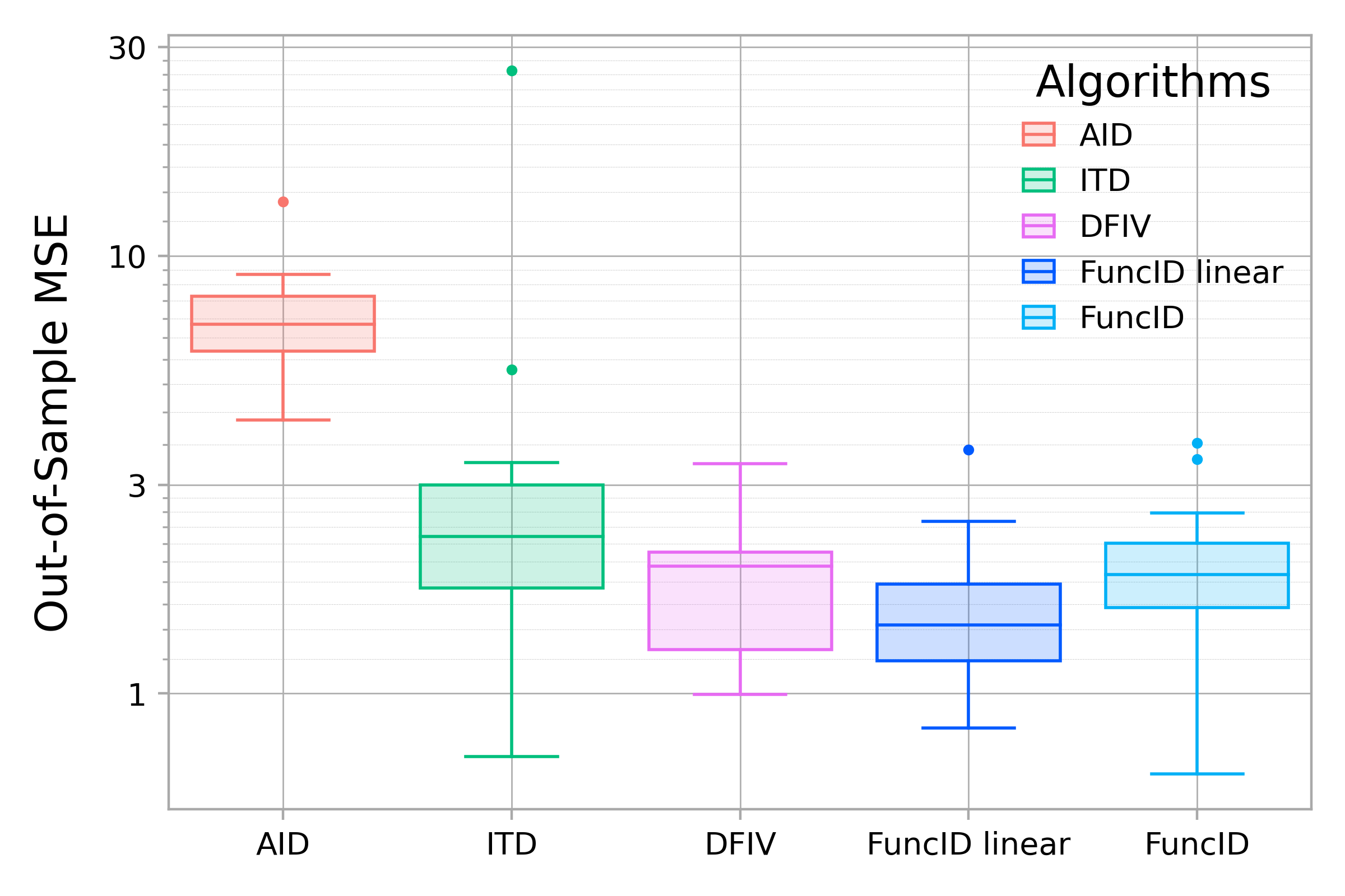
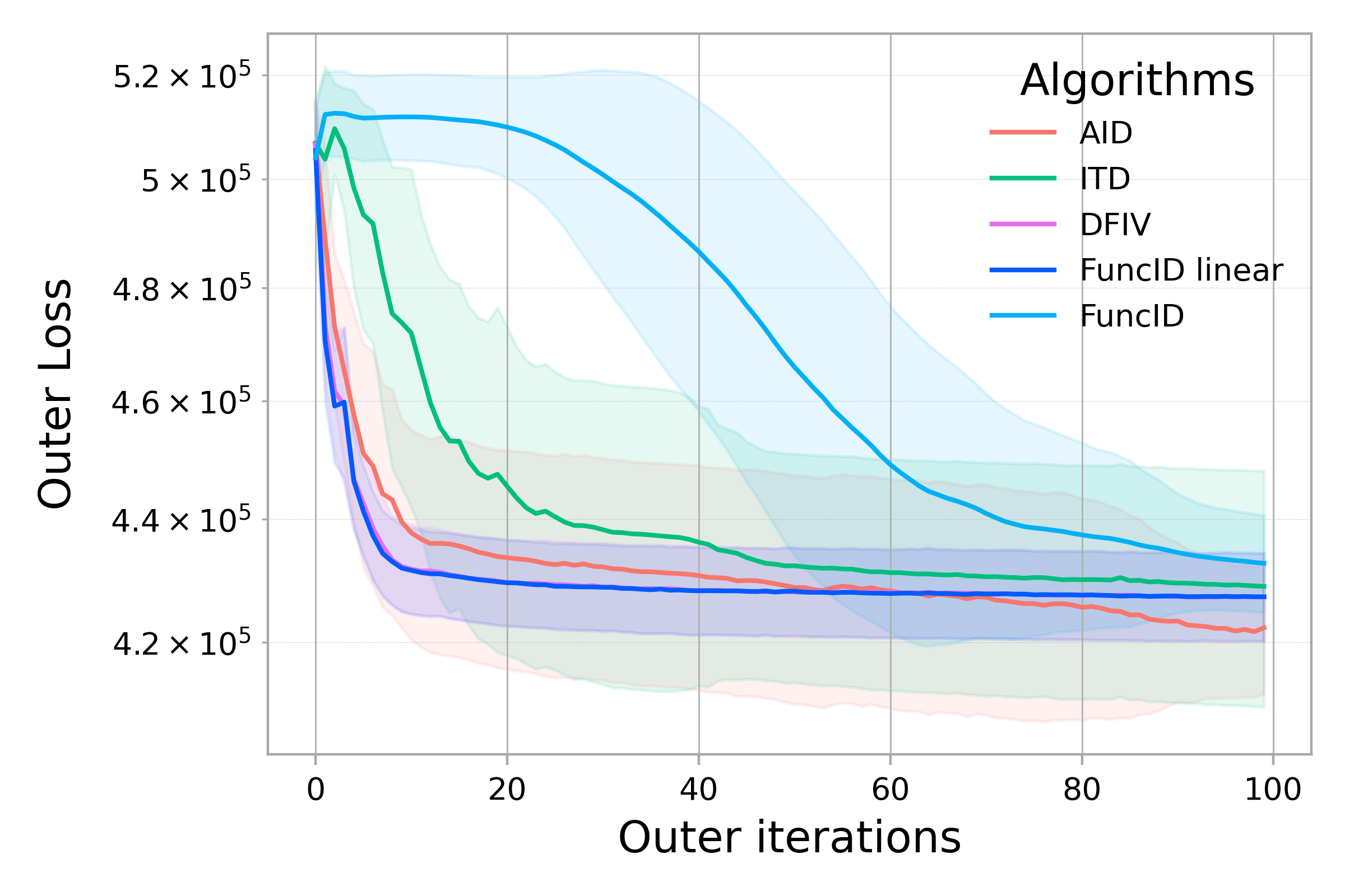
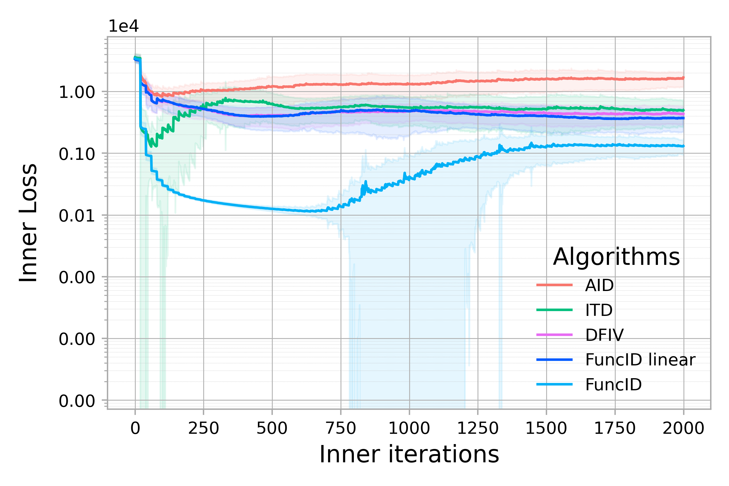
Figure 5: Performance metrics for Instrumental Variable (IV) regression. (Right) final test loss. (Middle) outer loss vs training iterations, (Right) inner loss vs training iterations, All results are averaged over 20 runs with 10000 training samples and 588 test samples.

Appendix F Model-based RL Experiments

F.1 Closed-form expression for the adjoint function

For the FuncID method, we exploit the structure of the adjoint objective to obtain a closed-form expression of the adjoint function $a_{\omega}^{\star}$. In the model-based RL setting, the unregularized adjoint objective has a simple expression of the form:

$$\hat{L}_{adj}(\omega,a,\hat{h}_{\omega},\mathcal{B})= \frac{1}{2\left\lvert\mathcal{B}_{in}\right\rvert}\sum_{(x,y)\in\mathcal{B}_{in}}\left\lVert a(x)\right\rVert^{2}$$ (53)

$$+\frac{1}{\left\lvert\mathcal{B}_{out}\right\rvert}a(x)^{\top}\partial_{v}f(\hat{h}_{\omega}(x),y).$$ (54)

The key observation here is that the same batches of data are used for both the inner and outer problems, i.e. $\mathcal{B}_{in}=\mathcal{B}_{out}$. Therefore, we only need to evaluate the function $a$ on a finite set of points $x$ where $(x,y)\in\mathcal{B}_{in}$. Without restricting the solution set of $a$ or adding regularization to $\hat{L}_{adj}$, the optimal solution $a_{\omega}^{\star}$ simply matches $-\partial_{v}f(\hat{h}_{\omega}(x),y)$ on the set of points $x$ s.t. $(x,y)\in\mathcal{B}_{in}$. Our implementation directly exploits this observation and uses the following expression for the total gradient estimation:

$$g_{out}=-\sum_{(x,y)\in\mathcal{B}_{in}}\partial_{\omega,v}f(\hat{h}_{\omega}(x),r_{\omega}(x),s_{\omega}(x))\partial_{v}f(\hat{h}_{\omega}(x),y).$$ (55)

F.2 Experimental details

As in the experiments of Nikishin et al. [2022], we use the CartPole environment with 2 actions, 4-dimensional continuous state space, and optimal returns of 500. For evaluation, we use a separate copy of the environment. The reported return is an average of 10 runs with different seeds.

Networks.

We us the same neural network architectures that are used in the CartPole experiment of Nikishin et al. [2022, Appendix D]. All networks have two hidden layers and ReLU activations. Both hidden layers in all networks have dimension 32. In the misspecified setting with the limited model class capacity, we set the hidden layer dimension to 3 for the dynamics and reward networks.

Hyper-parameters.

We perform 200000 environment steps (outer-level steps) and set the number of inner-level iterations to $M=1$ for both OMD and funcID. for MLE, we perform a single update to the state-value function for each update to the model. For training, we use a replay buffer with a batch size of 256, and set the discount factor $\gamma$ to $0.99$. When sampling actions, we use a temperature parameter $\alpha=0.01$ as in Nikishin et al. [2022]. The learning rate for outer parameters $\omega$ is set to $10^{-3}$. For the learning rate of the inner neural network and the moving average coefficient $\tau$, we perform a grid search over $\left\{10^{-4},10^{-3},3\cdot 10^{-3}\right\}$ and $\{5\cdot 10^{-3},10^{-2}\}$ as in Nikishin et al. [2022].

F.3 Additional results

Time comparison.

Figure 6 shows the average reward on the evaluation environment as a function of training time in seconds. We observe that our model is the fastest to reach best performance both in the well-specified and misspecified settings.

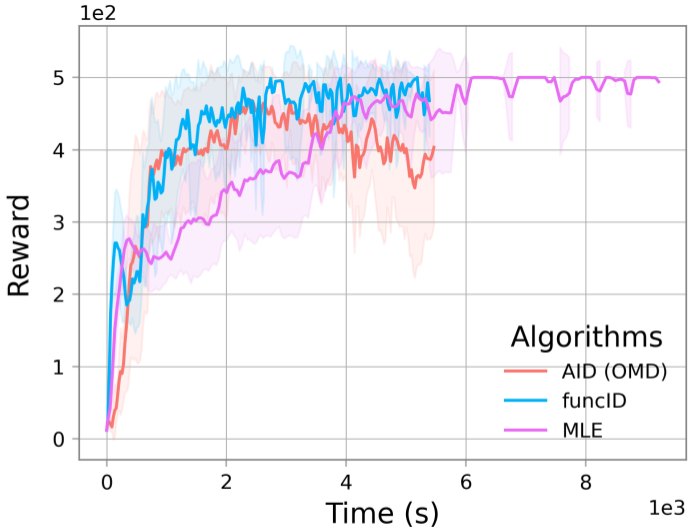
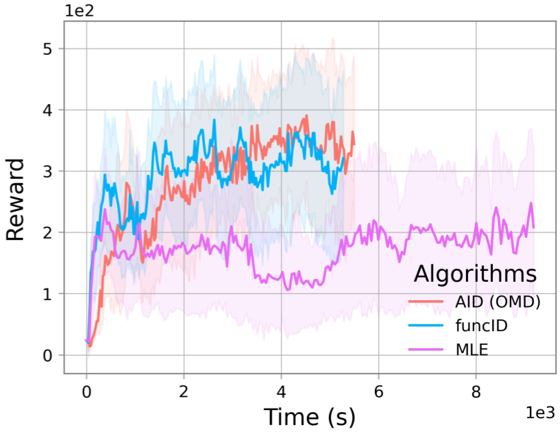
Figure 6: Average Reward on an evaluation environment vs. time in seconds on the CartPole task. (Left) Well-specified predictive model with 32 hidden units to capture the variability in the states dynamics. (Right) misspecified predictive model with only 3 hidden states.

MDP model comparison.

Figure 7 shows the average prediction error of different methods during training. The differences in average prediction error between the bilevel approaches (OMD, FuncID) and MLE reflect their distinct optimization objectives and trade-offs. OMD and FuncID focus on maximizing performance in the task environment, while MLE emphasizes accurate representation of all aspects of the environment, which can lead to smaller prediction errors but may not necessarily correlate with superior evaluation performance. We also observe that FuncID has a stable prediction error in both settings meanwhile OMD and MLE exhibit some instability.

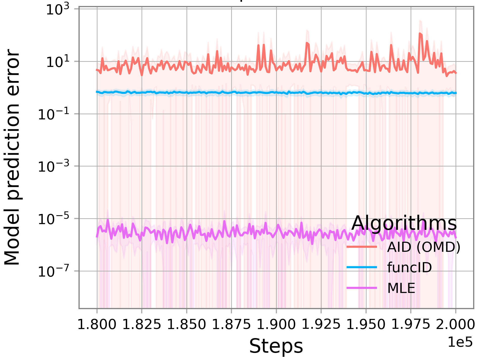
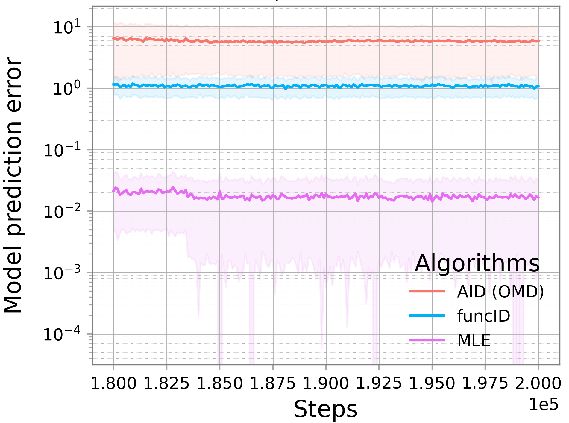
Figure 7: Average MDP model prediction error in the training environment vs. inner optimization steps on the CartPole task. (Left) Well-specified predictive model with 32 hidden units to capture the variability in the states dynamics. (Right) misspecified predictive model with only 3 hidden states.

References

• Ablin et al. [2020] P. Ablin, G. Peyré, and T. Moreau. Super-efficiency of automatic differentiation for functions defined as a minimum. International Conference on Machine Learning (ICML), 2020.
• Ahuja et al. [2020] K. Ahuja, K. Shanmugam, K. Varshney, and A. Dhurandhar. Invariant risk minimization games. International Conference on Machine Learning (ICML), 2020.
• Amos et al. [2023] B. Amos et al. Tutorial on amortized optimization. Foundations and Trends® in Machine Learning, 16(5):592–732, 2023.
• Arbel and Mairal [2022a] M. Arbel and J. Mairal. Amortized implicit differentiation for stochastic bilevel optimization. International Conference on Learning Representations (ICLR), 2022a.
• Arbel and Mairal [2022b] M. Arbel and J. Mairal. Non-convex bilevel games with critical point selection maps. Advances in Neural Information Processing Systems (NeurIPS), 2022b.
• Arjovsky et al. [2019] M. Arjovsky, L. Bottou, I. Gulrajani, and D. Lopez-Paz. Invariant risk minimization. arXiv preprint 1907.02893, 2019.
• Bae and Grosse [2020] J. Bae and R. B. Grosse. Delta-stn: Efficient bilevel optimization for neural networks using structured response jacobians. Advances in Neural Information Processing Systems (NeurIPS), 2020.
• Bansal et al. [2023] D. Bansal, R. T. Chen, M. Mukadam, and B. Amos. Taskmet: Task-driven metric learning for model learning. Advances in Neural Information Processing Systems (NeurIPS), 2023.
• Bauschke and Combettes [2011] H. H. Bauschke and P. L. Combettes. Convex Analysis and Monotone Operator Theory in Hilbert Spaces. Springer Publishing Company, Incorporated, 1st edition, 2011. ISBN 1441994661.
• Baydin et al. [2017] A. G. Baydin, B. A. Pearlmutter, A. A. Radul, and J. M. Siskind. Automatic differentiation in machine learning: A survey. Journal of Machine Learning Research (JMLR), 18(153):1–43, 2017.
• Bengio et al. [1994] Y. Bengio, P. Simard, and P. Frasconi. Learning long-term dependencies with gradient descent is difficult. IEEE Transactions on Neural Networks, 5(2):157–166, 1994.
• Bennett et al. [2006] K. P. Bennett, J. Hu, X. Ji, G. Kunapuli, and J.-S. Pang. Model selection via bilevel optimization. IEEE International Joint Conference on Neural Network Proceedings, 2006.
• Bertinetto et al. [2019] L. Bertinetto, J. F. Henriques, P. H. Torr, and A. Vedaldi. Meta-learning with differentiable closed-form solvers. International Conference on Learning Representations (ICLR), 2019.
• Bińkowski et al. [2018] M. Bińkowski, D. J. Sutherland, M. Arbel, and A. Gretton. Demystifying mmd gans. arXiv preprint arXiv:1801.01401, 2018.
• Blondel et al. [2022] M. Blondel, Q. Berthet, M. Cuturi, R. Frostig, S. Hoyer, F. Llinares-López, F. Pedregosa, and J.-P. Vert. Efficient and modular implicit differentiation. Advances in Neural Information Processing Systems (NeurIPS), 2022.
• Blundell et al. [2007] R. Blundell, X. Chen, and D. Kristensen. Semi-nonparametric iv estimation of shape-invariant engel curves. Econometrica, 75(6):1613–1669, 2007.
• Blundell et al. [2012] R. Blundell, J. L. Horowitz, and M. Parey. Measuring the price responsiveness of gasoline demand: Economic shape restrictions and nonparametric demand estimation. Quantitative Economics, 3(1):29–51, 2012.
• Bollen [2012] K. A. Bollen. Instrumental variables in sociology and the social sciences. Annual Review of Sociology, 38:37–72, 2012.
• Bolte et al. [2021] J. Bolte, T. Le, E. Pauwels, and T. Silveti-Falls. Nonsmooth implicit differentiation for machine-learning and optimization. Advances in Neural Information Processing Systems (NeurIPS), 2021.
• Bolte et al. [2024] J. Bolte, E. Pauwels, and S. Vaiter. One-step differentiation of iterative algorithms. Advances in Neural Information Processing Systems (NeurIPS), 2024.
• Bottou [2010] L. Bottou. Large-scale machine learning with stochastic gradient descent. International Conference on Computational Statistics (COMPSTAT), 2010.
• Bradbury et al. [2018] J. Bradbury, R. Frostig, P. Hawkins, M. J. Johnson, C. Leary, D. Maclaurin, G. Necula, A. Paszke, J. VanderPlas, S. Wanderman-Milne, and Q. Zhang. JAX: composable transformations of Python+NumPy programs, 2018. URL http://github.com/google/jax.
• Brock et al. [2018] A. Brock, T. Lim, J. Ritchie, and N. Weston. SMASH: One-shot model architecture search through hypernetworks. International Conference on Learning Representations (ICLR), 2018.
• Brockman et al. [2016] G. Brockman, V. Cheung, L. Pettersson, J. Schneider, J. Schulman, J. Tang, and W. Zaremba. Openai gym. arXiv preprint 1606.01540, 2016.
• Cawley and Meyerhoefer [2012] J. Cawley and C. Meyerhoefer. The medical care costs of obesity: an instrumental variables approach. Journal of Health Economics, 31(1):219–230, 2012.
• Chen et al. [2018] R. T. Chen, Y. Rubanova, J. Bettencourt, and D. K. Duvenaud. Neural ordinary differential equations. Advances in Neural Information Processing Systems (NeurIPS), 2018.
• Debnath and Mikusinski [2005] L. Debnath and P. Mikusinski. Introduction to Hilbert spaces with applications. Academic press, 2005.
• Dempe et al. [2007] S. Dempe, J. Dutta, and B. Mordukhovich. New necessary optimality conditions in optimistic bilevel programming. Optimization, 56(5-6):577–604, 2007.
• Domke [2012] J. Domke. Generic methods for optimization-based modeling. International Conference on Artificial Intelligence and Statistics (AISTATS), 2012.
• Fang and Santos [2018] Z. Fang and A. Santos. Inference on Directionally Differentiable Functions. The Review of Economic Studies, 86(1):377–412, 2018.
• Feurer and Hutter [2019] M. Feurer and F. Hutter. Hyperparameter optimization. Springer International Publishing, 2019.
• Franceschi et al. [2017] L. Franceschi, M. Donini, P. Frasconi, and M. Pontil. Forward and reverse gradient-based hyperparameter optimization. International Conference on Machine Learning (ICML), 2017.
• Fu et al. [2022] Z. Fu, Z. Qi, Z. Wang, Z. Yang, Y. Xu, and M. R. Kosorok. Offline reinforcement learning with instrumental variables in confounded markov decision processes. arXiv preprint 2209.08666, 2022.
• Ghadimi and Wang [2018] S. Ghadimi and M. Wang. Approximation methods for bilevel programming. Optimization and Control, 2018.
• Goodman [1971] V. Goodman. Quasi-differentiable functions of banach spaces. Proceedings of the American Mathematical Society, 30(2):367–370, 1971.
• Gould et al. [2016] S. Gould, B. Fernando, A. Cherian, P. Anderson, R. S. Cruz, and E. Guo. On differentiating parameterized argmin and argmax problems with application to bi-level optimization. arXiv preprint 1607.05447, 2016.
• Grazzi et al. [2020] R. Grazzi, L. Franceschi, M. Pontil, and S. Salzo. On the iteration complexity of hypergradient computation. International Conference on Machine Learning (ICML), 2020.
• Ha et al. [2017] D. Ha, A. M. Dai, and Q. V. Le. Hypernetworks. International Conference on Learning Representations (ICLR), 2017.
• Holler et al. [2018] G. Holler, K. Kunisch, and R. C. Barnard. A bilevel approach for parameter learning in inverse problems. Inverse Problems, 34(11):115012, 2018.
• Hong et al. [2023] M. Hong, H. Wai, Z. Wang, and Z. Yang. A two-timescale stochastic algorithm framework for bilevel optimization: Complexity analysis and application to actor-critic. SIAM Journal on Optimization, 33(1):147–180, 2023.
• Hu et al. [2023] Y. Hu, J. Wang, Y. Xie, A. Krause, and D. Kuhn. Contextual stochastic bilevel optimization. Advances in Neural Information Processing Systems (NeurIPS), 2023.
• Ioffe and Tihomirov [1979] A. D. Ioffe and V. M. Tihomirov. Theory of Extremal Problems. Series: Studies in Mathematics and its Applications 6. Elsevier, 1979.
• Ji et al. [2021] K. Ji, J. Yang, and Y. Liang. Bilevel optimization: Convergence analysis and enhanced design. International Conference on Machine Learning (ICML), 2021.
• Jia and Benson [2019] J. Jia and A. R. Benson. Neural jump stochastic differential equations. Advances in Neural Information Processing Systems (NeurIPS), 2019.
• Kingma and Ba [2015] D. P. Kingma and J. Ba. Adam: A method for stochastic optimization. International Conference on Learning Representations (ICLR), 2015.
• Kingma and Welling [2014] D. P. Kingma and M. Welling. Auto-encoding variational bayes. International Conference on Learning Representations (ICLR), 2014.
• Kunapuli et al. [2008] G. Kunapuli, K. Bennett, J. Hu, and J.-S. Pang. Bilevel model selection for support vector machines. CRM Proceedings and Lecture Notes, 45:129–158, 2008.
• Kwon et al. [2024] J. Kwon, D. Kwon, S. Wright, and R. D. Nowak. On penalty methods for nonconvex bilevel optimization and first-order stochastic approximation. International Conference on Learning Representations (ICLR), 2024.
• Li et al. [2023] S. Li, Z. Wang, A. Narayan, R. Kirby, and S. Zhe. Meta-learning with adjoint methods. International Conference on Artificial Intelligence and Statistics (AISTATS), 2023.
• Li et al. [2020] X. Li, T.-K. L. Wong, R. T. Chen, and D. Duvenaud. Scalable gradients for stochastic differential equations. International Conference on Artificial Intelligence and Statistics (AISTATS), 2020.
• Liao et al. [2018] R. Liao, Y. Xiong, E. Fetaya, L. Zhang, K. Yoon, X. Pitkow, R. Urtasun, and R. Zemel. Reviving and improving recurrent back-propagation. International Conference on Machine Learning (ICML), 2018.
• Liu et al. [2021a] R. Liu, X. Liu, S. Zeng, J. Zhang, and Y. Zhang. Value-function-based sequential minimization for bi-level optimization. IEEE Transactions on Pattern Analysis and Machine Intelligence (PAMI), 45:15930–15948, 2021a.
• Liu et al. [2021b] R. Liu, Y. Liu, S. Zeng, and J. Zhang. Towards gradient-based bilevel optimization with non-convex followers and beyond. Advances in Neural Information Processing Systems (NeurIPS), 2021b.
• Liu et al. [2022] R. Liu, J. Gao, J. Zhang, D. Meng, and Z. Lin. Investigating bi-level optimization for learning and vision from a unified perspective: a survey and beyond. IEEE Transactions on Pattern Analysis and Machine Intelligence (PAMI), 44:10045–10067, 2022.
• Liu et al. [2023] R. Liu, Y. Liu, W. Yao, S. Zeng, and J. Zhang. Averaged method of multipliers for bi-level optimization without lower-level strong convexity. International Conference on Machine Learning (ICML), 2023.
• Lorraine et al. [2019] J. Lorraine, P. Vicol, and D. K. Duvenaud. Optimizing millions of hyperparameters by implicit differentiation. International Conference on Artificial Intelligence and Statistics (AISTATS), 2019.
• MacKay et al. [2019] M. MacKay, P. Vicol, J. Lorraine, D. Duvenaud, and R. B. Grosse. Self-tuning networks: Bilevel optimization of hyperparameters using structured best-response functions. International Conference on Learning Representations (ICLR), 2019.
• Mairal et al. [2012] J. Mairal, F. Bach, and J. Ponce. Task-driven dictionary learning. IEEE Transactions on Pattern Analysis and Machine Intelligence (PAMI), 34(4):791–804, 2012.
• Margossian and Betancourt [2021] C. C. Margossian and M. Betancourt. Efficient automatic differentiation of implicit functions. arXiv preprint 2112.14217, 2021.
• Marrie et al. [2023] J. Marrie, M. Arbel, D. Larlus, and J. Mairal. Slack: Stable learning of augmentations with cold-start and kl regularization. Conference on Computer Vision and Pattern Recognition (CVPR), 2023.
• Matthey et al. [2017] L. Matthey, I. Higgins, D. Hassabis, and A. Lerchner. dsprites: Disentanglement testing sprites dataset, 2017.
• Nagendra et al. [2017] S. Nagendra, N. Podila, R. Ugarakhod, and K. George. Comparison of reinforcement learning algorithms applied to the cart-pole problem. International Conference on Advances in Computing, Communications and Informatics (ICACCI), 2017.
• Navon et al. [2021] A. Navon, I. Achituve, H. Maron, G. Chechik, and E. Fetaya. Auxiliary learning by implicit differentiation. International Conference on Learning Representations (ICLR), 2021.
• Nemirovski and Semenov [1973] A. Nemirovski and S. Semenov. On polynomial approximation of functions on hilbert space. Mathematics of the USSR-Sbornik, 21(2):255, 1973.
• Nikishin et al. [2022] E. Nikishin, R. Abachi, R. Agarwal, and P.-L. Bacon. Control-oriented model-based reinforcement learning with implicit differentiation. AAAI Conference on Artificial Intelligence, 2022.
• Noll [1993] D. Noll. Second order differentiability of integral functionals on Sobolev spaces and L2-spaces. Walter de Gruyter, Berlin/New York Berlin, New York, 1993.
• Pascanu et al. [2013] R. Pascanu, T. Mikolov, and Y. Bengio. On the difficulty of training recurrent neural networks. International Conference on Machine Learning (ICML), 2013.
• Paszke et al. [2019] A. Paszke, S. Gross, F. Massa, A. Lerer, J. Bradbury, G. Chanan, T. Killeen, Z. Lin, N. Gimelshein, L. Antiga, A. Desmaison, A. Kopf, E. Yang, Z. DeVito, M. Raison, A. Tejani, S. Chilamkurthy, B. Steiner, L. Fang, J. Bai, and S. Chintala. Pytorch: An imperative style, high-performance deep learning library. Advances in Neural Information Processing Systems (NeurIPS), 2019.
• Pedregosa [2016] F. Pedregosa. Hyperparameter optimization with approximate gradient. International Conference on Machine Learning (ICML), 2016.
• Pontryagin [2018] L. S. Pontryagin. Mathematical Theory of Optimal Processes. Routledge, 2018.
• Rezende et al. [2014] D. J. Rezende, S. Mohamed, and D. Wierstra. Stochastic backpropagation and approximate inference in deep generative models. International Conference on Machine Learning (ICML), 2014.
• Robbins and Monro [1951] H. Robbins and S. Monro. A stochastic approximation method. The Annals of Mathematical Statistics, pages 400–407, 1951.
• Rosset [2008] S. Rosset. Bi-level path following for cross validated solution of kernel quantile regression. International Conference on Machine Learning (ICML), 2008.
• Shaban et al. [2019] A. Shaban, C.-A. Cheng, N. Hatch, and B. Boots. Truncated back-propagation for bilevel optimization. International Conference on Artificial Intelligence and Statistics (AISTATS), 2019.
• Singh et al. [2019] R. Singh, M. Sahani, and A. Gretton. Kernel instrumental variable regression. Advances in Neural Information Processing Systems (NIPS), 2019.
• Stock and Trebbi [2003] J. H. Stock and F. Trebbi. Retrospectives: Who invented instrumental variable regression? Journal of Economic Perspectives, 17(3):177–194, 2003.
• Suonperä and Valkonen [2024] E. Suonperä and T. Valkonen. Linearly convergent bilevel optimization with single-step inner methods. Computational Optimization and Applications, 87(2):571–610, 2024.
• Sutton [1991] R. S. Sutton. Dyna, an integrated architecture for learning, planning, and reacting. ACM Sigart Bulletin, 2(4):160–163, 1991.
• van der Vaart [1991] A. van der Vaart. Efficiency and hadamard differentiability. Scandinavian Journal of Statistics, 18(1):63–75, 1991.
• van der Vaart and Wellner [1996] A. W. van der Vaart and J. A. Wellner. Weak Convergence and Empirical Processes with Applications to Statistics, pages 16–28. Springer New York, 1996.
• Vicol et al. [2021] P. Vicol, J. Lorraine, D. Duvenaud, and R. Grosse. Implicit regularization in overparameterized bilevel optimization. International Conference on Machine Learning (ICML), 2022.
• Von Stackelberg [2010] H. Von Stackelberg. Market Structure and Equilibrium. Springer Science & Business Media, 2010.
• Williams and Seeger [2000] C. Williams and M. Seeger. Using the nyström method to speed up kernel machines. Advances in Neural Information Processing Systems (NIPS), 2000.
• Williams and Peng [1990] R. J. Williams and J. Peng. An efficient gradient-based algorithm for on-line training of recurrent network trajectories. Neural Computation, 2(4):490–501, 1990.
• Xu et al. [2021a] L. Xu, Y. Chen, S. Srinivasan, N. de Freitas, A. Doucet, and A. Gretton. Learning deep features in instrumental variable regression. International Conference on Learning Representations (ICLR), 2021a.
• Xu et al. [2021b] L. Xu, H. Kanagawa, and A. Gretton. Deep proxy causal learning and its application to confounded bandit policy evaluation. Advances in Neural Information Processing Systems (NeurIPS), 2021b.
• Ye and Ye [1997] J. Ye and X. Ye. Necessary optimality conditions for optimization problems with variational inequality constraints. Mathematics of Operations Research, 22(4):977–997, 1997.
• Ye and Zhu [1995] J. Ye and D. Zhu. Optimality conditions for bilevel programming problems. Optimization, 33(1):9–27, 1995.
• Ye et al. [1997] J. Ye, D. Zhu, and Q. J. Zhu. Exact penalization and necessary optimality conditions for generalized bilevel programming problems. SIAM Journal on Optimization, 7(2):481–507, 1997.
• Zhang et al. [2019] C. Zhang, M. Ren, and R. Urtasun. Graph hypernetworks for neural architecture search. International Conference on Learning Representations (ICLR), 2019.
• Zhong et al. [2019] Y. D. Zhong, B. Dey, and A. Chakraborty. Symplectic ode-net: Learning hamiltonian dynamics with control. arXiv preprint 1909.12077, 2019.