High-dimensional analysis of ridge regression for non-identically distributed data with a variance profile

Abstract

High-dimensional linear regression has been thoroughly studied in the context of independent and identically distributed data. We propose to investigate high-dimensional regression models for independent but non-identically distributed data. To this end, we suppose that the set of observed predictors (or features) is a random matrix with a variance profile and with dimensions growing at a proportional rate. Assuming a random effect model, we study the predictive risk of the ridge estimator for linear regression with such a variance profile. In this setting, we provide deterministic equivalents of this risk and of the degree of freedom of the ridge estimator. For certain class of variance profile, our work highlights the emergence of the well-known double descent phenomenon in high-dimensional regression for the minimum norm least-squares estimator when the ridge regularization parameter goes to zero. We also exhibit variance profiles for which the shape of this predictive risk differs from double descent. The proofs of our results are based on tools from random matrix theory in the presence of a variance profile that have not been considered so far to study regression models. Numerical experiments are provided to show the accuracy of the aforementioned deterministic equivalents on the computation of the predictive risk of ridge regression. We also investigate the similarities and differences that exist with the standard setting of independent and identically distributed data.

Keywords: High-dimensional linear ridge regression; Non-identically distributed data; Degrees of freedom; Double descent; Variance profile; Heteroscedasticity; Random Matrices; Deterministic equivalents.

1 Introduction

High-dimensionality is a subject of interest in the field of statistics, especially in regression problems, driven by the advent of massive data sets. This context gives rise to unexpected phenomena and contradictions with established statistical heuristics when the dimension $p$ of the predictors is fixed and the number $n$ of observations tends to infinity. These phenomena particularly appear in the context of linear regression. Indeed, as the sample size and dimension of acquired data increase, the study of this model is different from the classical framework. In the asymptotic regime where $\min(n,p)\to+\infty$ and $\frac{p}{n}\to c>0$, one can notably mention the occurrence of the double descent phenomenon corresponding to estimators that both interpolates the data and show good generalization performances [BHMM19]. In this asymptotic setting, using tools from random matrix theory (RMT), many authors have therefore focused on the consequences of high-dimensionality on linear regression, see e.g. [DW18, Bac24, HMRT22, LC18] and references therein. In this paper, we focus on the linear regression model

$$Y_{n}=X_{n}\theta_{\ast}+\varepsilon_{n},$$ (1.1)

where $X_{n}$ is $n\times p$ matrix of random predictors, $\varepsilon_{n}\in{\mathbb{R}}^{n}$ is a noise vector independent of $X_{n}$ with $\mathbb{E}[\varepsilon_{n}]=0$ and $\mathbb{E}[\varepsilon_{n}\varepsilon_{n}^{t}]=\sigma^{2}I_{n}$, $\theta_{\ast}\in{\mathbb{R}}^{p}$ is a vector of unknown parameters, and $Y_{n}\in{\mathbb{R}}^{n}$ is the vector of observed responses.

Classically, the predictors are assumed to be independent and identically distributed (iid) data, meaning that the rows of the matrix $X_{n}$ are independent vectors sampled from the same probability distribution. In this paper, we propose to depart from this assumption by considering the setting where the rows of $X_{n}$ are independent but non-identically distributed. To this end, we suppose that $X_{n}$ is expressed in the following form

$$X_{n}=\Upsilon_{n}\circ Z_{n},$$

where $\circ$ denotes the Hadamard product between two matrices, $Z_{n}=(Z_{ij})$ has iid centered entries with variance one, and $\Upsilon_{n}=(\gamma_{ij}^{(n)})$ is a deterministic matrix. To simplify the notation, we shall sometimes write $\gamma_{ij}^{(n)}=\gamma_{ij}$ and thus drop the (possibly) dependence of $\gamma_{ij}$ on $n$. The matrix

$$\Gamma_{n}=(\gamma_{ij}^{2})\in{\mathbb{R}}^{n\times p}$$

governs the variance of the entries of $X_{n}$, and it is called a variance profile.

In the RMT literature, there exist various works on the analysis of the spectrum of large random matrices with a variance profile [Shl96, HLN07, ACD⁺21, BM20, EYY12, AEK17a]. In particular, we rely on results from [HLN07] to obtain a deterministic equivalent of the spectral distribution of a data matrix $X_{n}=\Upsilon_{n}\circ Z_{n}$ with a variance profile matrix $\Gamma_{n}$. The motivation for studying linear regression using such a variance profile is to consider the setting where one has $n$ independent pairs of observations $(Y_{i},X_{i})_{1\leq i\leq n}$ (with $X_{i}=(X_{ij})_{1\leq j\leq p}$) that are not necessarily identically distributed. Note that in the standard setting of iid data, one that

$$\gamma_{ij}=\gamma_{j}\quad\mbox{for all}\quad 1\leq i\leq n,\mbox{ and }1\leq j\leq p.$$

The main goal of this paper is then to understand how assuming such a variance profile for $X_{n}$ influences the statistical properties of ridge regression in the linear model (1.1) when compared to the standard assumption of iid observations. In this setting, our approach also allows to analyze the performances of the minimum norm least-squares estimator when the ridge regularization parameter goes to zero.

We consider the high-dimensional context (with $p$ growing to infinity at a rate proportional to $n$) for which the least squares estimator is possibly not uniquely defined. Thus, we focus our analysis on the ridge regression estimator that is the minimizer of the following loss function

$$\hat{\theta}_{\lambda}=\operatorname*{arg\,min}_{\theta\in{\mathbb{R}}^{p}}\frac{1}{n}\|Y_{n}-X_{n}\theta\|^{2}+\lambda\|\theta\|^{2},$$

for some regularization parameter $\lambda>0$. Regardless of the ratio between $n$ and $p$, this estimator has the following explicit expression

$$\hat{\theta}_{\lambda}=(X^{t}_{n}X_{n}+n\lambda I_{p})^{-1}X_{n}^{t}Y_{n}=X_{n}^{t}(X_{n}X_{n}^{t}+n\lambda I_{n})^{-1}Y_{n}.$$ (1.2)

Our analysis also includes the study of the minimum least-square estimator defined as

$$\hat{\theta}=\operatorname*{arg\,min}_{\theta\in{\mathbb{R}}^{p}}\left\{\|\theta\|\;:\;\theta\mbox{ minimizes }\frac{1}{n}\|Y_{n}-X_{n}\theta\|^{2}\right\},$$

to which the ridge regression estimator converges when $\lambda$ tends to zero. The estimator $\hat{\theta}$ is also known to be the solution found by gradient descent when initialized to zero, see e.g. [HMRT22][Proposition 1].

To study the statistical performances of the ridge regression estimator, we analyse its predictive risk defined as

$$\hat{r}_{\lambda}(X_{n})=\mathbb{E}[(\widetilde{Y}-\widetilde{X}^{t}\hat{\theta}_{\lambda})^{2}|X_{n}],$$ (1.3)

where $(\widetilde{Y},\widetilde{X})\in{\mathbb{R}}\times{\mathbb{R}}^{p}$ is independent from $(Y_{n},X_{n})$ and satisfies

$$\widetilde{Y}=\widetilde{X}^{t}\theta_{\ast}+\tilde{\varepsilon},\mbox{ with }\mathbb{E}[\tilde{\varepsilon}]=0,\;\mathbb{E}[\tilde{\varepsilon}^{2}]=\sigma^{2}\ \mathrm{and}\ \widetilde{X},\ \tilde{\varepsilon}\ \mathrm{independent}.$$

In the above formula, $\widetilde{X}=\widetilde{S}_{p}^{1/2}\widetilde{Z}$ with $\widetilde{Z}\in{\mathbb{R}}^{p}$ a random vector with iid centered entries and variance one, and

$$\widetilde{S}_{p}=\mathbb{E}[\widetilde{X}\widetilde{X}^{t}]=\mathop{\rm diag}\nolimits(\tilde{\gamma}_{1}^{2},\ldots,\tilde{\gamma}_{p}^{2})$$

denotes the variance profile of $\widetilde{X}$. Note that the risk $\hat{r}_{\lambda}(X_{n})$ is conditioned on the predictors $X_{n}$, and it is thus a random variable.

Following [DW18], we focus on a random-effect hypothesis by assuming that the components of the vector $\theta_{\ast}$ are drawn independently at random. As argued in [DW18], this assumption corresponds to an average case analysis over a set of dense regression coefficients as opposed to the “sparsity hypothesis” [HTW15] or the “manifold hypothesis” [LHT23] that are other popular assumptions in high-dimensional linear regression. More precisely, the following random coefficients assumption is made throughout the paper.

Assumption 1.1.

The vector $\theta_{\ast}$ of regression coefficients is random, independent from $X_{n}$, $\widetilde{X}$, $\varepsilon_{n}$ and $\tilde{\varepsilon}$, with $\mathbb{E}[\theta_{\ast}]=0$ and

$$\mathbb{E}[\theta_{\ast}\theta_{\ast}^{t}]=\frac{\alpha^{2}}{p}I_{p}.$$

The above coefficient $\alpha>0$ represents the average amount of signal strength in model (1.1). Under Assumption 1.1, the expectation in (1.3) used to define the predictive risk is thus taken with respect to both the randomness of the vector of coefficients $\theta_{\ast}$, the vector $\widetilde{X}$ and the additive noise $\varepsilon_{n}$ and $\tilde{\varepsilon}$.

1.1 Main contributions

Recall that the estimation of $Y_{n}$ by ridge regression is

$$\hat{Y}_{\lambda}=X_{n}\hat{\theta}_{\lambda}=A_{\lambda}Y_{n},\quad\mbox{where}\quad A_{\lambda}=X_{n}(X^{t}_{n}X_{n}+n\lambda I_{p})^{-1}X_{n}^{t}.$$

Then, the so-called degrees of freedom (DOF) of the estimator $\hat{\theta}_{\lambda}$ that is defined as

$$\widehat{df}_{1}(\lambda)=\operatorname{Tr}[A_{\lambda}]=\operatorname{Tr}[\widehat{\Sigma}_{n}(\widehat{\Sigma}_{n}+\lambda I_{p})^{-1}],\mbox{ where }\widehat{\Sigma}_{n}=\frac{1}{n}X_{n}^{t}X_{n},$$

represents the so-called effective dimension of the linear estimator $\hat{Y}_{\lambda}$. The DOF is widely used in statistics to define various criteria for model selection among a collection of estimators, see e.g. [Efr04].

Inspired by recent results from [Bac24] in the setting of iid data, a first contribution of this work is to prove the following deterministic equivalence of the DOF

$$\widehat{df}_{1}(\lambda)\sim df_{1}(\lambda),\quad\mbox{where}\quad df_{1}(\lambda)=\operatorname{Tr}[\Sigma_{n}(\Sigma_{n}+\kappa(\lambda))^{-1}],$$ (1.4)

where

$$\Sigma_{n}=\mathbb{E}[\widehat{\Sigma}_{n}]=\frac{1}{n}\mathop{\rm diag}\nolimits\left(\sum_{i=1}^{n}\gamma^{2}_{i1},\ldots,\sum_{i=1}^{n}\gamma^{2}_{ip}\right),$$

and $\kappa(\lambda)$ is diagonal matrix that depends upon the regularization parameter $\lambda$ and the variance profile matrix $\Gamma_{n}$.

Throughout the paper, the meaning of the equivalence notation $A_{n}\sim B_{n}$ between two random variables is

$$\lim_{n\to\infty,\;p/n\to c}|A_{n}-B_{n}|=0,\;\mbox{almost surely}.$$

Hence, the equivalence relation (1.4) indicates that the DOF of the ridge regression estimator for the empirical covariance matrix $\widehat{\Sigma}_{n}$ corresponds to the DOF computed with its expected version $\Sigma_{n}$ (the usual population covariance matrix for iid data), and another additive regularization structure than $\lambda I_{p}$ that is given by the diagonal matrix $\kappa(\lambda)$ whose explicit expression is given in Section 3.

Then, the second and main contribution of the paper is to derive a deterministic equivalent of the predictive risk $\hat{r}_{\lambda}(X_{n})$ in the case where the number of samples $n$ and the dimension $p$ tend to infinity at a proportional rate, that is $\lim\limits_{n\to+\infty}\frac{p}{n}=c>0$. This deterministic equivalent allows us to understand the influence of the ratio $c$ on the predictive risk and to also analyze the effect of the signal strength $\alpha$. We also study the convergence of the predictive risk as $\lambda$ tends to $0$ to analyze the statistical properties the minimum norm least square estimator. In this setting, it appears a phenomenon arising from the curse of dimensionality that is commonly known as double descent for iid data. This phenomenon contradicts the consensus heuristic that, when a model becomes over-parameterized, then the predictive risk increases due to overfitting of the training data and the model is no longer capable of generalizing. This double descent has been thoroughly studied in the case of high-dimensional linear regression using tool from RMT, see e.g. [HMRT22, Bac24, BHX20] and references therein. In this paper, we show that it also occurs for non iid data with a variance profile. Our deterministic equivalent of the predictive risk also allows to derive the asymptotic behavior of an optimal choice for the regularization parameter and to compare it to the one obtained for iid data in [DW18].

As a third contribution, using synthetic data and various illustrative examples of variance profile, we conduct numerical experiments to verify the accuracy of our deterministic equivalent of the predictive risk using finite samples. We also investigate the similarities and differences that exist between the standard setting of iid data and the one of non-identically distributed data with a variance profile.

For example, if the variance profile is assumed to be quasi doubly stochastic in the sense that

$$\frac{1}{n}\sum_{j=1}^{p}\gamma_{ij}^{2}=\frac{p}{n},\mbox{ for all }1\leq i\leq n,\quad\mbox{and}\quad\frac{1}{n}\sum_{i=1}^{n}\gamma_{ij}^{2}=1,\mbox{ for all }1\leq j\leq p,$$

then, we prove in this paper that

$$\lim_{n\to\infty,\;p/n\to c}\hat{r}_{0}(X_{n})=\left\{\begin{array}[]{ccc}\sigma^{2}\frac{c}{1-c}+\sigma^{2}&\mbox{if}&c<1\\ \alpha^{2}\left(1-\frac{1}{c}\right)+\sigma^{2}\frac{1}{c-1}&\mbox{if}&c>1\end{array}\right.,\;\mbox{almost surely}.$$ (1.5)

The above result corresponds to the known asymptotic limit of the predictive risk of the minimum norm least squares estimator for iid data when the entries of $X_{n}$ are independent centered random variables with variance $1$, see e.g. [HMRT22], which is referred to as a constant variance profile in this paper (that is $\gamma_{ij}=1$). In this setting, the predictive risk of $\hat{\theta}$ is thus increasing with $p$ up to $p/n<1$ and then decreasing for $p>n$ (that is beyond the interpolation threshold $p=n$) which is classically referred to as the double descent phenomenon as illustrated in Figure 1(a).

By going beyond the quasi doubly stochastic assumption (1.5), the results of this paper, on the asymptotic limit of the predictive risk, also allow to exhibit variance profiles for which the predictive risk has a shape that differs from double descent. This is illustrated in Figure 1(b), where the deterministic equivalent of the predictive risk has a triple descent behavior (as a function of $p/n$) for the following piecewise constant variance profile

$$\Gamma_{n}=\left[\begin{array}[]{cc}\gamma_{1}^{2}\mathbbm{1}_{n/4}\mathbbm{1}_{p/4}^{t}&\gamma_{2}^{2}\mathbbm{1}_{n/4}\mathbbm{1}_{3p/4}^{t}\\ \gamma_{2}^{2}\mathbbm{1}_{3n/4}\mathbbm{1}_{p/4}^{t}&\gamma_{1}^{2}\mathbbm{1}_{3n/4}\mathbbm{1}_{3p/4}^{t}\end{array}\right],$$

where $\mathbbm{1}_{q}$ denotes the vector of length $q$ with all entries equal to one, and $\gamma_{1},\gamma_{2}$ are positive constant such that $\gamma_{2}\gg\gamma_{1}$. Note that Figure 1(b) also illustrates the accuracy of the deterministic equivalent of the predictive risk that is proposed in this paper.

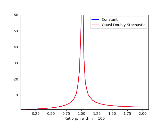
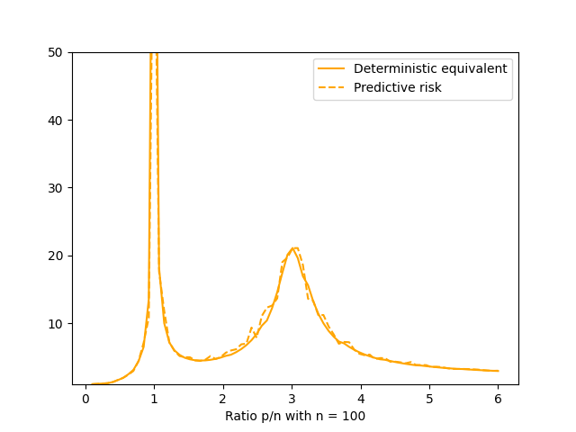
Figure 1: Predictive risk for several variance profiles with $\lambda=0$. (a) Comparison of constant and quasi doubly stochastic variance profiles with $\alpha=\sigma=1$, $n=100$ and $p$ varying from $10$ to $200$. (b) Piecewise constant variance profile with $\gamma_{1}^{2}=0.0005$, $\gamma_{2}^{2}=1$, $\alpha=\sigma=1$, $n=100$ and $p$ varying from $10$ to $600$.

1.2 Organisation of the paper

In Section 2, we review various works related to the analysis of high-dimensional linear regression and the study of random matrices with a variance profile. The main results are presented and discussed in Section 3. Numerical experiments are then reported in Section 4. A conclusion and some perspectives are proposed in Section 5. All proofs using tools from the theory of random matrices and operator-valued Stieltjes transforms are deferred to an Appendix where we also discuss the use of random matrices with a variance profile in free probability.

1.3 Publicly available source code

For the sake of reproducible research, a Python code is available at the following address:

https://github.com/Issoudab/RidgeRegressionVarianceProfile

to implement the experiments carried out in this paper.

2 Related works

In this section, we review the literature on the analysis of high-dimensional regression using tools from RMT. We also discuss existing works on linear regression for non-iid data, and the use of random matrices with a variance profile in statistics and RMT.

2.1 High-dimensional linear regression from the random matrix perspective

When the sample size is comparable to the dimensionality of the observations, recent advances in RMT have been successfully applied to various inference problems in high-dimensional multivariate statistics, see e.g. [NPW21] for a recent overview. Many works have considered the high-dimensional analysis of the linear model using tools from RMT for iid data with a general covariance structure $\Sigma\in{\mathbb{R}}^{p\times p}$ (assumed to be a positive semi-definite matrix) that is for

$$X_{n}=Z_{n}\Sigma^{1/2},\mbox{ for an $n\times p$ matrix $Z_{n}$ with iid centered entries having variance one.}$$

In particular, for such data, the study of the minimum norm least-square estimator and the double descent behavior of the predictive risk has been considered in [HMRT22, Bac24, BHX20, RMR21]. The analysis of the predictive risk of ridge regression using iid data with a general covariance structure has been studied in [DW18, Bac24], while previous works on the statistical analysis of ridge regression from the RMT perspective include [EK18, Dic16] and [CD11, TV04] for applications in wireless communication.

2.2 Linear regression for independent but non-identically distributed data

While the statistical analysis of linear regression for iid data with a general covariance structure is very well understood, the literature on the study of the linear model for non-identically distributed predictors appears to be scarcer. A first analysis of maximum likelihood estimation in standard models (including linear regression) for independent but non-identically distributed data dates back to [Ber82]. More recent works [BBK⁺19, KBB⁺20], on statistical inference in linear regression in the so-called model-free framework, allow to consider the setting on non-identically distributed predictors. However, to the best of our knowledge, the high-dimensional analysis of the linear model using non-identically distributed data has not considered so far.

2.3 The use of variance profile in RMT

RMT allows to describe the asymptotic distribution of the eigenvalues of large matrices with random entries, see e.g. [BS10]. In particular, the well-known Marchenko-Pastur theorem characterizes the limiting spectral distribution of the covariance matrix $\widehat{\Sigma}_{n}=\frac{1}{n}X_{n}^{t}X_{n}$ for a data matrix $X_{n}=Z_{n}\Sigma^{1/2}$ with iid rows in the asymptotic setting $\lim\limits_{n\to+\infty}\frac{p}{n}=c>0$.

However, in many applications, such as photon imaging [SHDW14], network traffic analysis [BMG13], ecology [AGB⁺15, AT15], neurosciences [ASS15, ARS15] or genomics for microbiome studies [CZL19], the amount of variance in the observed data matrix may significantly change from one sample to the other, that is between the rows of $X_{n}$. The literature on statistical inference from high-dimension matrices with heteroscedasticity has thus recently been growing [BM20, BDF17, LDS18, UHZB16, ZCW22, JFL22]. Modeling data as a random matrix $X_{n}=\Upsilon_{n}\circ Z_{n}$ with a variance profile to handle the setting of non-iid data has also found applications in the analysis of the performances of wireless digital communication channels [HLN07]. In the RMT literature, Hermitian random matrices with centered entries but non-equal distribution are referred to as generalized Wigner matrices for which many asymptotic properties are now well understood. For example, for Hermitian random matrices with a variance profile that is doubly stochastic (namely its rows and columns elements sump up to one), bulk universality at optimal spectral resolution for local spectral statistics have been established in [EYY12] and they are shown to converge to those of a standard Wigner matrix (that is with iid sub-diagonal entries). The case of a generalized Wigner matrix with a variance profile that is not necessarily doubly stochastic has been studied in [AEK17a], and non-herminitian random matrices with a variance profile have been considered in [CHNR18, HLN07, HLN06] using the notion of deterministic equivalent that consists in approximating the spectral distribution of a random matrix by a deterministic function.

Let us now recall the key notion of Stieltjes transform.

Definition 2.1.

Let $\mu$ be a probability measure supported on ${\mathbb{R}}$. Then, its Stieltjes transform is defined as

$$g_{\mu}(z)=\int_{{\mathbb{R}}}\frac{1}{t-z}d\mu(t),\quad\mbox{for}\quad t\in\mathbb{C}^{+},$$

where $\mathbb{C}^{+}=\{z\in\mathbb{C},\Im(z)>0\}$ and $\Im(\cdot)$ denotes the imaginary part of a complex number.

Then, we build upon results from [HLN07] to construct deterministic equivalents (when $\lim_{n\to+\infty}p/n\to c>0$) of the Stieltjes transforms

$$g_{\hat{\mu}_{n}}(z)=\frac{1}{p}\operatorname{Tr}[(\widehat{\Sigma}_{n}-zI_{p})^{-1}],\quad\mbox{for}\quad z\in\mathbb{C}\setminus{\mathbb{R}}^{+},$$

and

$$g_{\tilde{\mu}_{n}}(z)=\frac{1}{n}\operatorname{Tr}[(\widetilde{\Sigma}_{n}-zI_{n})^{-1}],\quad\mbox{for}\quad z\in\mathbb{C}\setminus{\mathbb{R}}^{+},$$

of the empirical eigenvalue distribution $\hat{\mu}_{n}$ of $\widehat{\Sigma}_{n}$, and the empirical eigenvalue distribution $\tilde{\mu}_{n}$ of $\widetilde{\Sigma}_{n}=\frac{1}{n}X_{n}X_{n}^{t}$ respectively.

To obtain these deterministic equivalents, the following assumptions will be needed, on mild moment conditions on the $Z_{ij}$’s and boundedness hypotheses on the entries of the variance profile matrix.

Assumption 2.1.

There exists $\delta>0$ such that, $\mathbb{E}[|Z_{ij}|^{4+\delta}]<+\infty,$ for all $1\leq i\leq n$ and $1\leq j\leq p$.

Assumption 2.2.

There exists $\gamma_{\mathrm{max}}>0$ such that, $\underset{n\geq 1}{\mathrm{sup}}\underset{\begin{subarray}{c}1\leq i\leq n\\ 1\leq j\leq p\end{subarray}}{\mathrm{max}}|\gamma_{ij}^{(n)}|<\gamma_{\mathrm{max}}.$

Assumption 2.3.

There exists $\gamma_{\mathrm{min}}>0$ such that, $\forall n\geq 1,\underset{\begin{subarray}{c}1\leq i\leq n\\ 1\leq j\leq n\end{subarray}}{\mathrm{min}}|\gamma_{ij}^{(n)}|\geq\gamma_{\mathrm{min}}.$

Assumption 2.4.

There exists $d_{\ast}>0$ such that, $|\frac{p}{n}-1|\geq d_{\ast}$ for all values of $n$ and $p$.

Throughout the paper, we also assume that $\widetilde{X}=\widetilde{S}_{p}^{1/2}\widetilde{Z}$ with

$$\mathbb{E}[|\widetilde{Z}_{j}|^{4+\delta}]<+\infty,\quad\underset{\begin{subarray}{c}1\leq j\leq p\end{subarray}}{\mathrm{max}}|\tilde{\gamma}_{j}^{(n)}|\leq\gamma_{\mathrm{max}}\;\mbox{and}\;\underset{\begin{subarray}{c}1\leq j\leq n\end{subarray}}{\mathrm{min}}|\tilde{\gamma}_{j}^{(n)}|\geq\gamma_{\mathrm{min}}$$

and for all $n\geq 1$. Then, using [HLN07][Theorem 2.5], the following result holds.

Proposition 2.1.

Under Assumptions 2.1-2.4, the following limit holds true almost surely

$$\lim_{n\to\infty,\;p/n\to c}\left(g_{\hat{\mu}_{n}}(z)-\frac{1}{p}\operatorname{Tr}[T_{p}(z)]\right)=0,\quad\mbox{for all}\quad z\in\mathbb{C}\setminus{\mathbb{R}}^{+},$$

$$\lim_{n\to\infty,\;p/n\to c}\left(g_{\tilde{\mu}_{n}}(z)-\frac{1}{n}\operatorname{Tr}[\widetilde{T}_{n}(z)]\right)=0,\quad\mbox{for all}\quad z\in\mathbb{C}\setminus{\mathbb{R}}^{+},$$

where

$$T_{p}(z)=\mathop{\rm diag}\nolimits(T_{p}^{(1)}(z),\ldots,T_{p}^{(p)}(z))\quad\mbox{and}\quad\widetilde{T}_{n}(z)=\mathop{\rm diag}\nolimits(\widetilde{T}_{n}^{(1)}(z),\ldots,\widetilde{T}_{n}^{(n)}(z)),$$

are diagonal matrices of size $p\times p$ and $n\times n$ respectively, whose diagonal elements are the unique solutions of the deterministic system of $p+n$ equations

$$T_{p}^{(j)}(z) = \frac{-1}{z(1+(1/n)\operatorname{Tr}[\widetilde{D}_{j}\widetilde{T}_{n}(z)])}\quad\mbox{for}\quad 1\leq j\leq p,$$ (2.1)

$$\widetilde{T}_{n}^{(i)}(z) = \frac{-1}{z(1+(1/n)\operatorname{Tr}[D_{i}T_{p}(z)])}\quad\mbox{for}\quad 1\leq i\leq n,$$ (2.2)

where

$$\widetilde{D}_{j}=\mathop{\rm diag}\nolimits(\gamma^{2}_{1j},\ldots,\gamma^{2}_{nj})\quad\mbox{and}\quad D_{i}=\mathop{\rm diag}\nolimits(\gamma^{2}_{i1},\ldots,\gamma^{2}_{ip}).$$

Moreover, $\frac{1}{p}\operatorname{Tr}[T_{p}(z)]$ and $\frac{1}{n}\operatorname{Tr}[\widetilde{T}_{n}(z)]$ are the Stieltjes transforms of probability measures denoted as $\nu_{n}$ and $\tilde{\nu}_{n}$ respectively.

The measures $\nu_{n}$ and $\tilde{\nu}_{n}$, defined in Proposition 2.1, are called the deterministic equivalents of the empirical eigenvalue distributions $\hat{\mu}_{n}$ and $\tilde{\mu}_{n}$ respectively. By a slight abuse of notation, we may also denote by $T_{p}(z)$ the vector of size $p$ whose entries are the coefficients $T_{p}^{(j)}(z)$ for $1\leq j\leq p$ solutions of the fixed point equations (2.1). Currently, a classical method to numerically approximate the value of $T_{p}(z)$ is to solve the nonlinear system of deterministic equations (2.1) written in a vector form that is referred to as the Dyson equation in [AEK17a, AEK19, AEK17b, AEK18]. Indeed, as stated in [AEK17b][Theorem 2.1], the vector $T_{p}(z)$ is known to be the unique solution of the Dyson equation

$$\frac{1}{T_{p}(z)}=-zI_{p}+\frac{1}{n}\Gamma_{n}^{t}\frac{1}{1+\frac{1}{n}\Gamma_{n}T_{p}(z)},$$ (2.3)

that corresponds to equations (2.1) and (2.2) written in a vector form, where $1/v$ has to be understood as taking the inverse of the elements of the vector $v$ entrywise. Similarly, the vector $\widetilde{T}_{n}(z)=(\widetilde{T}_{n}^{(i)}(z))_{1\leq i\leq n}$ satisfies the Dyson equation

$$\frac{1}{\widetilde{T}_{n}(z)}=-zI_{n}+\frac{1}{n}\Gamma_{n}\frac{1}{1+\frac{1}{n}\Gamma_{n}^{t}\widetilde{T}_{n}(z)}.$$

In this paper, we sometimes consider, as an illustrative example, a specific class of variance profiles said to be quasi doubly stochastic in the following sense.

Definition 2.2.

The variance profile $\Gamma_{n}$ is called quasi doubly stochastic when its rows and columns sum up to constant values (that are necessarily different when $n\neq p$), namely

$$\frac{1}{n}\sum_{j=1}^{p}\gamma_{ij}^{2}=\frac{p}{n},\mbox{ for all }1\leq i\leq n,\quad\mbox{and}\quad\frac{1}{n}\sum_{i=1}^{n}\gamma_{ij}^{2}=1,\mbox{ for all }1\leq j\leq p.$$

The fixed point equation (2.3) typically does not have an explicit expression, and one has to rely on numerical methods to solve it as done in Section 4. Nevertheless, when the variance profile is quasi doubly stochastic, the solution of the Dyson equation is a vector $T_{p}(z)$ having constant entries equal to $m_{p}(z)\in\mathbb{C}$ (or equivalently $T_{p}(z)=m_{p}(z)I_{p}$ is a scalar matrix) that satisfies

$$\frac{1}{m_{p}(z)}=-z+\frac{1}{1+\frac{p}{n}m_{p}(z)},\quad\mbox{for all}\quad z\in\mathbb{C}\setminus{\mathbb{R}}^{+}.$$ (2.4)

The above equality corresponds to the well-known fixed point equation satisfied by the Stieltjes transform $m_{p}(z)$ of the Marchenko-Pastur distribution [BS10]. One also has that $\widetilde{T}_{n}(z)=\tilde{m}_{n}(z)I_{n}$ with $\tilde{m}_{n}(z)$ satisfying

$$\frac{1}{\tilde{m}_{n}(z)}=-z+\frac{p/n}{1+\tilde{m}_{n}(z)},\quad\mbox{for all}\quad z\in\mathbb{C}\setminus{\mathbb{R}}^{+}.$$

3 Main results

In this section, we derive deterministic equivalents for the DOF and the predictive risk of ridge regression. We also obtain a deterministic equivalent of the predictive risk of minimum norm least square estimation when the ridge regularization parameter tends to zero. We compare these results to those that are already known in the standard setting of iid data, and we highlight the emergence of the double descent phenomenon for non-iid data. Throughout this section, it is supposed that Assumptions 2.1-2.4 hold true.

3.1 Degrees of freedom

In this section, we prove that the quantity $df_{1}(\lambda)$ introduced in Section 1.1 is a deterministic equivalent of the DOF $\widehat{df}_{1}(\lambda)$ .

Proposition 3.1.

For any $\lambda>0$, the following holds

$$\lim_{n\to\infty,\;p/n\to c}|\widehat{df}_{1}(\lambda)-df_{1}(\lambda)|=0,\;\mbox{almost surely},$$ (3.1)

with $df_{1}(\lambda)=\operatorname{Tr}[\Sigma_{n}(\Sigma_{n}+\kappa(\lambda))^{-1}]$, and

$$\kappa(\lambda) = \mathop{\rm diag}\nolimits(\kappa_{1}(\lambda),\ldots,\kappa_{p}(\lambda)),\quad\mbox{where}\quad\kappa_{j}(\lambda)=\frac{\operatorname{Tr}[\widetilde{D}_{j}]}{\operatorname{Tr}[\widetilde{D}_{j}\widetilde{T}_{n}(-\lambda)]},\quad\mbox{for}\quad 1\leq j\leq p.$$ (3.2)

When the variance profile is quasi doubly stochastic, one has that $\operatorname{Tr}[\widetilde{D}_{j}]=n$. Moreover, as remarked in Section 2.3, the matrix $\widetilde{T}_{n}(-\lambda)=\tilde{m}_{n}(-\lambda)I_{n}$ is scalar, implying that

$$\operatorname{Tr}[\widetilde{D}_{j}\widetilde{T}_{n}(-\lambda)]=n\tilde{m}_{n}(-\lambda),\quad\mbox{for all}\quad 1\leq j\leq p.$$

Moreover, in this setting, $\Sigma_{n}=I_{p}$. Consequently, if $\Gamma_{n}$ is quasi doubly stochastic, one has that

$$\kappa(\lambda)=\frac{1}{\tilde{m}_{n}(-\lambda)}I_{p},$$

and the deterministic equivalent of the DOF is

$$df_{1}(\lambda)=\operatorname{Tr}\left[\Sigma_{n}\left(\Sigma_{n}+\kappa(\lambda)\right)^{-1}\right]=p\left(1+\frac{1}{\tilde{m}_{n}(-\lambda)}\right)^{-1}.$$

The above equality corresponds to the formula of a deterministic equivalent of the DOF derived in [Bac24] for iid data when the entries of the features matrix $X_{n}$ are made of iid centered random variables with variances equal to $1$.

3.2 Predictive risk

We first express the predictive risk in a more convenient way. To this end, for any square matrix $A$, we denote by $\Delta[A]$ the diagonal matrix whose diagonal entries are those of $A$.

Lemma 3.1.

For any $\lambda>0$, the predicitive risk $\hat{r}_{\lambda}(X_{n})=\mathbb{E}[(\widetilde{Y}-\widetilde{X}^{t}\hat{\theta}_{\lambda})^{2}|X_{n}]$ has the following expression

$$\hat{r}_{\lambda}(X_{n}) = \sigma^{2}+\frac{\sigma^{2}}{n}\mathrm{Tr}\big{[}\widetilde{S}_{p}\Delta[Q_{p}(-\lambda)]\big{]}+\lambda\left(\frac{\lambda\alpha^{2}}{p}-\frac{\sigma^{2}}{n}\right)\mathrm{Tr}\big{[}\widetilde{S}_{p}\Delta[Q_{p}^{\prime}(-\lambda)]\big{]}.$$ (3.3)

Moreover, we can exhibit the following Bias-Variance decomposition for $\hat{r}_{\lambda}(X_{n})$ :

$$\hat{r}_{\lambda}(X_{n}) = \sigma^{2}+\mathrm{Bias}(\hat{\theta}_{\lambda})+\mathrm{Var}(\hat{\theta}_{\lambda}),$$

with

$$\mathop{\rm Bias}\nolimits(\hat{\theta}_{\lambda}) = \mathbb{E}\big{[}(\mathbb{E}[\hat{\theta}_{\lambda}|X_{n},\theta_{\ast}]-\theta_{\ast})^{t}\widetilde{S}_{p}(\mathbb{E}[\hat{\theta}_{\lambda}|X_{n},\theta_{\ast}]-\theta_{\ast})\big{|}X_{n}\big{]}$$

$$= \frac{\lambda^{2}\alpha^{2}}{p}\mathrm{Tr}\big{[}\widetilde{S}_{p}\Delta[Q_{p}^{\prime}(-\lambda)]\big{]},$$

and

$$\mathop{\rm Var}(\hat{\theta}_{\lambda}) = \mathbb{E}\big{[}(\hat{\theta}_{\lambda}-\mathbb{E}[\hat{\theta}_{\lambda}|X_{n},\theta_{\ast}])^{t}\widetilde{S}_{p}(\hat{\theta}_{\lambda}-\mathbb{E}[\hat{\theta}_{\lambda}|X_{n},\theta_{\ast}])\big{|}X_{n}\big{]}$$

$$= \frac{\sigma^{2}}{n}\mathrm{Tr}\big{[}\widetilde{S}_{p}\Delta[Q_{p}(-\lambda)]-\lambda\widetilde{S}_{p}\Delta[Q_{p}^{\prime}(-\lambda)]\big{]},$$

where

$$Q_{p}(z)=(\widehat{\Sigma}_{n}-zI_{p})^{-1}\quad\mbox{for}\quad z\in\mathbb{C}\setminus{\mathbb{R}}^{+},$$

is the resolvent of the matrix $\widehat{\Sigma}_{n}$, and $Q_{p}^{\prime}$ denotes the derivative of $Q_{p}$ with respect to $z$.

We can now give a deterministic equivalent of the predictive risk $\hat{r}_{\lambda}(X_{n})$ that is obtained in a simple way by replacing the diagonal matrix $\Delta[Q_{p}(z)]$ with the deterministic matrix $T_{p}(z)$ in the expression (3.3) of the predictive risk. All proofs of the following results are given in Appendix A.3.

Theorem 3.1.

A deterministic equivalent of the predictive risk is

$$r_{\lambda}(\Upsilon_{n})=\sigma^{2}+\frac{\sigma^{2}}{n}\mathrm{Tr}[\widetilde{S}_{p}T_{p}(-\lambda)]+\lambda\left(\frac{\lambda\alpha^{2}}{p}-\frac{\sigma^{2}}{n}\right)\mathrm{Tr}[\widetilde{S}_{p}T_{p}^{\prime}(-\lambda)],$$ (3.4)

in the sense that it satisfies

$$\lim_{n\to\infty,\;p/n\to c}|\hat{r}_{\lambda}(X_{n})-r_{\lambda}(\Upsilon_{n})|=0,\;\mbox{almost surely},$$

where $T_{p}^{\prime}(z)$ denotes the derivative of $T_{p}(z)$ with respect to $z$.

A key argument to derive the computation of $r_{\lambda}(\Upsilon_{n})$ is to prove that the matrix $T_{p}(z)$ is a relevant deterministic equivalent of the diagonal matrix $\Delta[Q_{p}(z)]$ for an appropriate notion of asympotic equivalence between matrices of growing size. This is the purpose of Apppendix A.2 where we derive a stronger convergence result than the one stated in Proposition 2.1 which only shows that $\frac{1}{p}\operatorname{Tr}[T_{p}(z)]$ is a deterministic equivalent of $g_{\hat{\mu}_{n}}(z)=\frac{1}{p}\operatorname{Tr}[Q_{p}(z)]$.

Lemma 3.2.

If $\frac{p}{n}<1$ then $T_{p}(-\lambda)$ and its derivative, $T_{p}^{\prime}(-\lambda)$ admit a limit when $\lambda$ tends to $0$. Indeed, there exists a constant $\tau>0$ such that

$$\lim_{\lambda\rightarrow 0,\;\lambda>0}T_{p}(-\lambda)=\int_{\tau}^{+\infty}\frac{\mu(dw)}{w}\quad\mathrm{and}\quad\lim_{\lambda\rightarrow 0,\;\lambda>0}T_{p}^{\prime}(-\lambda)=\int_{\tau}^{+\infty}\frac{\mu(dw)}{w^{2}},$$

where $\mu=(\mu_{ij})$ is a positive $p\times p$ matrix valued-measure such that $\mu_{ii}$ is a probability measure and $\mu_{ij}$ is a null measure if $i\neq j$. We denote these limits by $T_{p}(0^{-})=\lim\limits_{\lambda\rightarrow 0}T_{p}(-\lambda)$ and $T_{p}^{\prime}(0^{-})=\lim\limits_{\lambda\rightarrow 0}T_{p}^{\prime}(-\lambda)$.

On the other hand, if $\frac{p}{n}>1$ then $\kappa(\lambda)$ and its derivative $\kappa^{\prime}(\lambda)$ also admit a limit when $\lambda$ tends to $0$ and we denote these limits by

$$\kappa(0^{+})=\lim_{\lambda\rightarrow 0,\;\lambda>0}\kappa(\lambda)\quad\mathrm{and}\quad\kappa^{\prime}(0^{+})=\lim_{\lambda\rightarrow 0,\;\lambda>0}\kappa^{\prime}(\lambda),$$

were $\kappa(\lambda)$ is the diagonal matrix defined in Equation (3.2).

Corollary 3.1.

Suppose that the variance profile $\Gamma_{n}$ is quasi doubly stochastic. Then, if $\frac{p}{n}<1$, one has that

$$T_{p}(0^{-})=m_{p}(0)I_{p},$$

and, if $\frac{p}{n}>1$,

$$\kappa(0^{+})=\frac{1}{\tilde{m}_{n}(0)}I_{p}\quad\mathrm{and}\quad\kappa^{\prime}(0^{+})=\frac{\tilde{m}_{n}^{\prime}(0)}{\tilde{m}_{n}^{2}(0)}I_{p},$$

where $m_{p}(.)$, resp. $\tilde{m}_{n}(.)$, is the Stieltjes transform of the Marchenko-Pastur distribution with parameter $p/n$, resp. $n/p$.

Then, Theorem 3.1 allows us to understand the behavior of $r_{\lambda}(\Upsilon_{n})$ when $\lambda\rightarrow 0$ and $\lambda\rightarrow+\infty$ through the following corollary.

Corollary 3.2.

As $\lambda\rightarrow+\infty$, the limit of the deterministic equivalent $r_{\lambda}(\Upsilon_{n})$ of the predictive risk is

$$\lim_{\lambda\rightarrow+\infty}r_{\lambda}(\Upsilon_{n})=\frac{\alpha^{2}}{p}\mathrm{Tr}[\widetilde{S}_{p}]+\sigma^{2}.$$

Moreover, as $\lambda\rightarrow 0$, the limit of the deterministic equivalent $r_{\lambda}(\Upsilon_{n})$ is as follows

-

if $\frac{p}{n}<1$ then

$$\lim_{\lambda\rightarrow 0,\;\lambda>0}r_{\lambda}(\Upsilon_{n})=\frac{\sigma^{2}}{n}\mathrm{Tr}[\widetilde{S}_{p}T_{p}(0^{-})]+\sigma^{2},$$

-

if $\frac{p}{n}>1$ then

$$\lim_{\lambda\rightarrow 0,\;\lambda>0}r_{\lambda}(\Upsilon_{n})=\frac{\alpha^{2}}{p}\mathrm{Tr}[\widetilde{S}_{p}\kappa(0^{+})(\Sigma_{n}+\kappa(0^{+}))^{-1}]+\frac{\sigma^{2}}{n}\mathrm{Tr}[\kappa^{\prime}(0^{+})\widetilde{S}_{p}\Sigma_{n}(\Sigma_{n}+\kappa(0^{+}))^{-2}]+\sigma^{2},$$

where $\kappa^{\prime}(\lambda)$ denotes the derivative with respecto to $\lambda$ of the diagonal matrix $\kappa(\lambda)$ defined in Equation (3.2).

In the case $\lambda\rightarrow 0$, Corollary 3.2 yields a deterministic equivalent of the predicitve risk of the mininum norm least-square estimator $\hat{\theta}$. Then, it can be seen that the risk $r_{0}(\Upsilon_{n})$ exhibit two different behaviors depending on the value of the ratio $p/n$ with respect to one.

If $p/n<1$, then $\hat{\theta}$ is equivalent to the ordinary least-square estimator $(X_{n}^{t}X_{n})^{-1}X_{n}^{t}Y_{n}$ which is known to be unbiased, and the risk $r_{0}(\Upsilon_{n})$ is thus only composed of a variance term. Moreover, if the variance profile is assumed to be quasi-bistochastic, then, given that

$$T_{p}(0^{-})=m_{p}(0)I_{p}\quad\mbox{and}\quad m_{p}(0)=\frac{1}{1-p/n},$$

it follows that

$$r_{0}(\Upsilon_{n})=\frac{\sigma^{2}}{1-p/n}\times\frac{1}{n}\mathrm{Tr}[\widetilde{S}_{p}]+\sigma^{2}=\sigma^{2}\frac{p/n}{1-p/n}+\sigma^{2}\rightarrow\sigma^{2}\frac{c}{1-c}+\sigma^{2},\;\mbox{as}\;n\to\infty,\;p/n\to c,$$

which corresponds, when $c<1$, to the known asymptotic limit of the predictive risk of least squares estimation for iid data when the entries of the features matrix $X_{n}$ are iid centered random variables with variances equal to $1$, see e.g. [HMRT22][Proposition 2].

If $p/n>1$, then the deterministic equivalent of the predictive risk is composed of a bias term and a variance term. If the variance profile is assumed to be quasi-bistochastic, the values of these two terms can be made more explicity as follows. In this setting, given that $\Sigma_{n}=I_{p}$, $\tilde{m}_{p}(0)=\frac{1}{p/n-1}$ and $\tilde{m}^{\prime}_{p}(0)=\frac{p/n}{(p/n-1)^{3}}$, one has that

$$\kappa(0^{+})=(p/n-1)I_{p}\quad\mathrm{and}\quad\kappa^{\prime}(0^{+})=\frac{p/n}{p/n-1}I_{p}.$$

Hence, using that $\frac{1}{n}\mathrm{Tr}[\widetilde{S}_{p}]=p/n$, we finally obtain that

$$r_{0}(\Upsilon_{n})=\alpha^{2}\left(1-\frac{n}{p}\right)+\sigma^{2}\frac{1}{p/n-1}\rightarrow\alpha^{2}\left(1-\frac{1}{c}\right)+\sigma^{2}\frac{1}{c-1},\;\mbox{as}\;n\to\infty,\;p/n\to c,$$

which corresponds, when $c>1$, to known results on the bias-variance decomposition of the asymotitic limit of the predictive risk of the minimum norm least squares estimator for iid data when the entries of $X_{n}$ are iid centered random variables with variance $1$, see e.g. [HMRT22][Theorem 1].

Beyond the assumption of a quasi-stochastic variance profile, it is difficult to analytically determine the shape of the preditive risk $r_{0}(\Upsilon_{n})$ as a function of the ratio $p/n$. Indeed, this requires to at least know upper and lower bounds on the magnitude of the diagonal elements of $T_{p}(0^{-})$ and $\kappa(0^{+})$ (and its derivative). As shown by Lemma 3.2 when $p/n<1$, this issue amounts to finding upper and lower bounds of the support of the matrix-valued measure $\mu$ satisfying

$$T_{p}(-0)=\int_{\tau}^{+\infty}\frac{\mu(dw)}{w}.$$

Hence, upper and lower bounding $T_{p}(-0)$ is related to understanding the value of the constant $\tau$ and the size of the support of the limiting spectral distribution of the covariance matrice $\Sigma_{n}$ which remains (to the best of our knowledge) an open problem for random matrices with an arbitrary variance profile.

Nevertheless, in Section 4, we use Corollary 3.2 and computational methods to evaluate $T_{p}(0^{-})$ and $\kappa(0^{+})$ to report numerical experiments illustrating that the double descent phenomemum for the predictive risk of $\hat{\theta}$ also holds in the high-dimensional model (1.1) with more general variance profile than a quasi-bistochastic one. In Section 4, we also exhibit variance profiles for which the predictive risk has a shape that differs from double descent.

Corollary 3.3.

The function $\lambda\mapsto\hat{r}_{\lambda}(X_{n})$ reaches its minimium at $\lambda_{\ast}=\frac{\sigma^{2}p}{\alpha^{2}n}$ meaning that

$$\hat{r}_{\lambda_{\ast}}(X_{n})\leq\hat{r}_{\lambda}(X_{n}),$$ (3.5)

for any $\lambda>0$.

Note that although $\hat{r}_{\lambda}(X_{n})$ depends on the variance profile, this is not the case of the optimal value of $\lambda_{\ast}$ that minimizes the predictive risk as shown by Corollary 3.3. Moreover, the optimal value $\lambda_{\ast}$ is also the one minimizing $\lambda\mapsto\hat{r}_{\lambda}(X_{n})$ in the framework of [DW18] with a matrix $X_{n}$ of features made of iid rows.

4 Numerical experiments

In this section, we illustrate the results of this paper with numerical experiments. Although we do not have an explicit formula for $T_{p}(z)$, this matrix-valued function satisfies the fixed-point equation (2.3). This allows us to approximate $T_{p}(z)$ numerically using a fixed-point algorithm. In this manner, we are thus able to obtain a numerical approximation of the deterministic equivalent $r_{\lambda}(\Upsilon_{n})$ of the predictive risk. In this section, we consider several variance profiles that we normalize such that

$$\frac{1}{n}\sum_{i=1}^{n}\sum_{j=1}^{p}\frac{\gamma^{2}_{ij}}{p}=1.$$

Apart from the constant, quasi doubly stochastic, and piecewise constant variance profiles mentioned earlier, we will use the following examples of variance profiles:

-

The alternated columns variance profile satisfying $\gamma_{ij}=\gamma_{1}$ if $j$ is even and $\gamma_{ij}=\gamma_{2}$ if $j$ is odd.

-

The polynomial variance profile satisfying $\gamma_{ij}^{2}=|i-j|^{6}+\tau$ for some $\tau>0$.

-

The block variance profile

$$\Gamma_{n}=\left[\begin{array}[]{ccc}\gamma_{1}^{2}\mathbbm{1}_{n/4}\mathbbm{1}_{p/4}^{t}&\gamma_{2}^{2}\mathbbm{1}_{n/4}\mathbbm{1}_{p/3}^{t}&\mathbbm{1}_{n/4}\mathbbm{1}_{5p/12}^{t}\\ \gamma_{2}^{2}\mathbbm{1}_{n/3}\mathbbm{1}_{p/4}^{t}&\gamma_{1}^{2}\mathbbm{1}_{n/3}\mathbbm{1}_{p/3}^{t}&\gamma_{3}^{2}\mathbbm{1}_{n/3}\mathbbm{1}_{5p/12}^{t}\\ \mathbbm{1}_{5n/12}\mathbbm{1}_{p/4}^{t}&\gamma_{3}^{2}\mathbbm{1}_{5n/12}\mathbbm{1}_{p/3}^{t}&\gamma_{1}^{2}\mathbbm{1}_{5n/12}\mathbbm{1}_{5p/12}^{t}\end{array}\right],$$

for some sufficiently different constants $\gamma_{1},\gamma_{2},\gamma_{3}$.

-

A variance profile referred to as the Berlin Photo for which $\gamma_{ij}$ is equal to the value of the coordinate $(i,j)$ of the pixel of the image depicted in Figure 2. The original image being of size $1250\times 850$, it is rescaled according to the values of $n$ and $p$ used in the numercial experiments thanks to the function resize from the Python module PIL.Image.

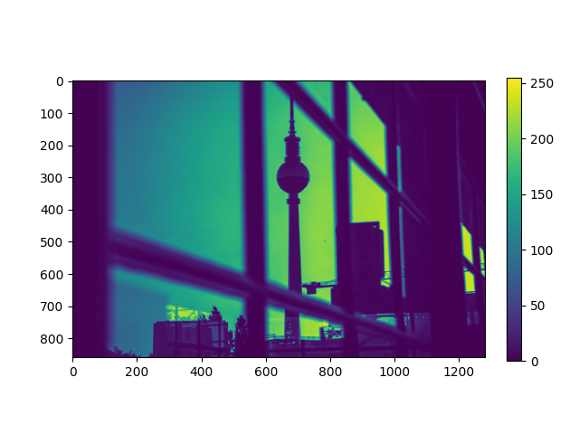
Figure 2: The Berlin Photo variance profile whose entries correspond to the the green channel of the pixels of a RGB picture taken in Berlin.

The values of the predictive risk and its deterministic equivalent are compared for various variance profiles in Figure 3 with $\lambda$ ranging from 0.1 to 10, $n=400$ and $p=600$. The curves displayed in Figure 3 confirm that $r_{\lambda}(\Upsilon_{n})$ is a very accurate estimator of $\hat{r}_{\lambda}(X_{n})$ in high-dimension since the dashed and solid lines coincide. These variance profiles also provide curves of predictive risks having similar shapes (up to a vertical translation). The curves representing the cases of constant and quasi doubly stochastic variance profile coincide, confirming the comment made in Section 1.1 on the doubly stochastic profile and its similarities with the setting of iid data. Moreover, the minimum of $r_{\lambda}(\Upsilon_{n})$ is indeed reached at the optimal value $\lambda_{\ast}$ for any variance profile as shown by Corollary 3.3.

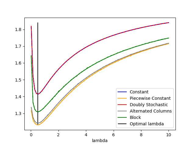
Figure 3: Comparison of $\hat{r}_{\lambda}(X_{n})$ and $r_{\lambda}(\Upsilon_{n})$ for several variance profiles , $\alpha=1$, $\sigma=1$, $n=400$ and $p=600$. The dashed lines correspond to the predictive risk while the solid lines correspond to the deterministic equivalent.

We illustrate the appearance of a double or triple descent phenomenon for several variance profiles in Figure 4 (a), (c) and (e). These figures represent the predictive risk and its approximation by a deterministic equivalent for various values of the ratio $p/n$ with $\lambda=0$. The solid lines depicts $r_{0}(\Upsilon_{n})$ whereas the dashed lines represent $\hat{r}_{0}(X_{n})$. For every variance profile, the solid and dashed lines coincide which confirms that $r_{0}(\Upsilon_{n})$ is a relevant deterministic equivalent of $\hat{r}_{0}(X_{n})$. For the constant and quasi doubly stochastic variance profiles, we observe the well known double descent phenomenon as illustrated by Figure 4 (a) since the curves are increasing for $p/n<1$ and decreasing for $p/n>1$. This is related to Corollary 3.2 which states that the expression of $\lim_{\lambda\rightarrow 0}r_{\lambda}(\Upsilon_{n})$ depends upon the value of the ratio $p/n$ with respect to one. Nevertheless, for other variance profiles, the shape of the predictive risk can be very different from one variance profile to another, and it differs from the usual double descent. For some variance profiles a phenomenon of triple descent arises, notably for the piecewise constant and block cases, as shown in Figure 4 (c) and (e). We also remark the appearance of a quadruple descent in the case of the polynomial profile, as shown in Figure 4 (e).

As already remarked at the end of Section 3, it is difficult to analytically explain these phenomenon for an arbitrary variance profile since we do not have an explicit formula for $T_{p}(z)$ in the general case. Nevertheless, as nicely discussed in [SKR⁺23], the double descent phenomenon is very much related to the distance from zero of the smallest non-negative eigenvalue of $\widehat{\Sigma}_{n}$. Having this eigenvalue close to zero causes double descent. In Figure 4 (b), (d) and (f), we thus represent the smallest non-zero eigenvalue $\tau_{\min}(\widehat{\Sigma}_{n})$ of $\widehat{\Sigma}_{n}$ for many variance profiles as a function of $p/n$. It can be observed that all the curves $p/n\to\tau_{\min}(\widehat{\Sigma}_{n})$ reach their minima at a value close to zero when $p=n$ where the double descent occurs, which is consistent with previous assertions in [SKR⁺23]. These curves in the constant and quasi doubly stochastic cases behave in a similar same way. However, one can remark from Figure 4 (f) that, for the piecewise constant and polynomial variance profiles, the value of $\tau_{\min}(\widehat{\Sigma}_{n})$ stay much closer to $0$ when $p/n$ is between $0.25$ and $3$ than in the constant or quasi doubly stochastic cases. The fact that these curves have a plateau near zero for $p/n\in[0.25,3]$ may be related to the appearance of the triple and quadruple descent phenomenon that is observed in Figure 4 (e).

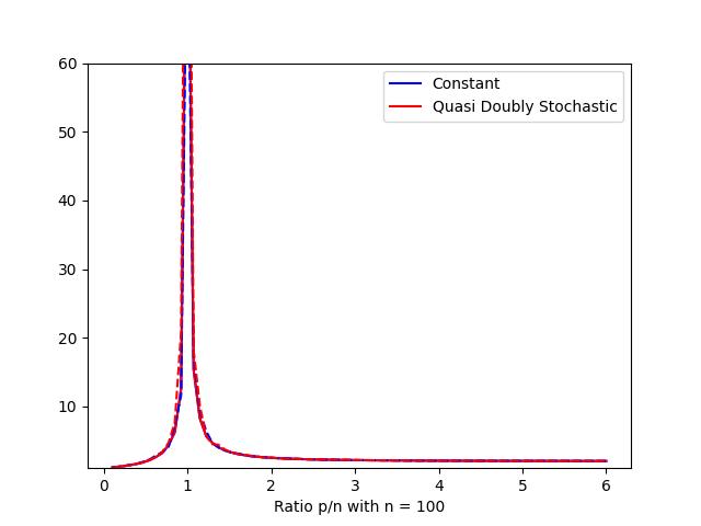
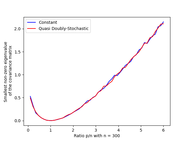
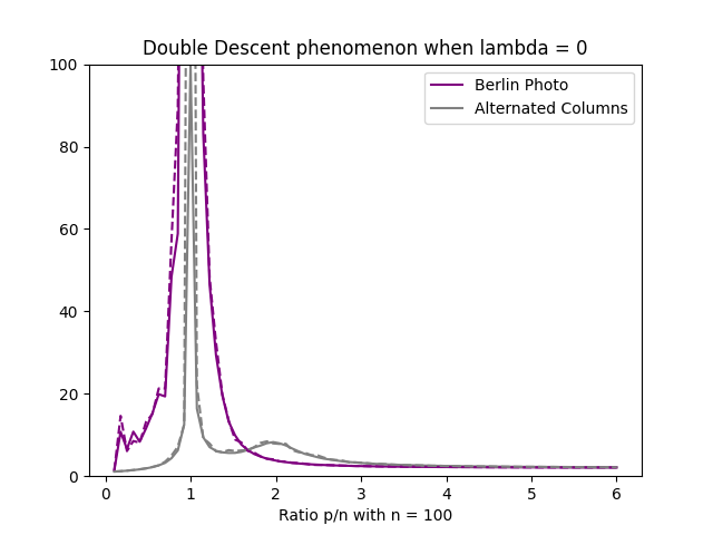
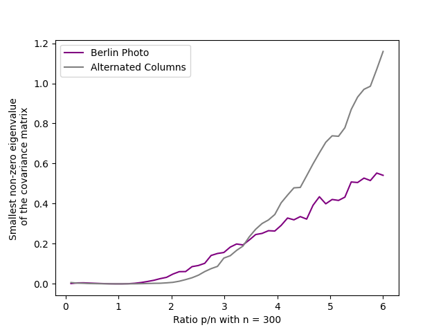
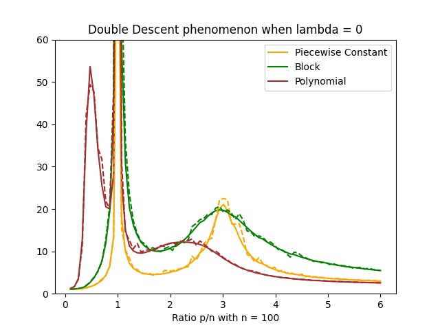
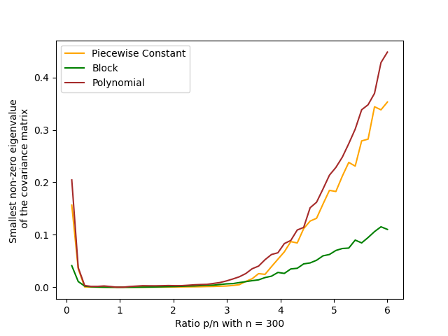
Figure 4: Left : Double descent phenomenon for several variance profiles with $\alpha=\sigma=1$, $n=100$ and $p$ varying from $10$ to $600$. Right : Smallest non-zero eigenvalue of $\widehat{\Sigma}_{n}$ for several variance profiles with $\alpha=\sigma=1$, $n=300$ and $p$ varying from $30$ to $1800$.

5 Conclusion

In this paper, we have derived a deterministic equivalent of the DOF and the predictive risk of ridge (less) regression in a high-dimensional framework with a variance profile to handle the setting of non-iid data. In order to achieve this result, we had to use ingredients from RMT to determine a deterministic equivalent of the diagonal of $Q_{p}(z)$. We have shown that results on the values of the DOF and the predictive that are already known for a constant variance profile, notably those of [DW18] and [Bac24], also hold in the case of a quasi doubly stochastic profile. However, there are variance profiles that cause a behavior of the predictive risk of the minimum norm least square estimator that differs from the double descent phenomenon as classically observed in the case of a constant variance profile. The numerical experiments that we have conducted confirm that our deterministic equivalent accurately estimates the predictive risk in high-dimension. Our results also allow to understand how assuming such a variance profile for the data influences the statistical properties of ridge regression when compared to the standard assumption of iid observations. We hope that our approach on the use of variance profiles may lead to further research works on the statistical analysis of other estimators than ridge regression in more complex models with non-iid data.

Appendix

In this appendix, we give all the proofs of the results of the paper. We also discuss the link between random matrices with a variance profile and the notion of $\mathcal{R}$-transform in free probability.

A.1 Proofs of Proposition 3.1 and Lemma 3.1

Proof of Proposition 3.1.

Recall that $\frac{1}{p}\widehat{df}_{1}(\lambda)=\frac{1}{p}\operatorname{Tr}[\widehat{\Sigma}_{n}(\widehat{\Sigma}_{n}+\lambda I_{p})^{-1}]$, for $\lambda>0$. Thus by using $\hat{\mu}_{n}$ the empirical eigenvalue distribution of $\widehat{\Sigma}_{n}$ we have this new expression of the degree of freedom

$$\frac{1}{p}\widehat{df}_{1}(\lambda)=\int_{{\mathbb{R}}}\frac{t}{t+\lambda}d\hat{\mu}_{n}(t).$$

Moreover, $\hat{\mu}_{n}$ being a probability measure one can notice from Definition 2.1 that

$$\frac{1}{p}\widehat{df}_{1}(\lambda)=\int_{{\mathbb{R}}}1-\frac{\lambda}{t+\lambda}d\hat{\mu}_{n}(t)=1-\lambda g_{\hat{\mu}_{n}}(-\lambda).$$

Thanks to Proposition 2.1, one has that

$$\frac{1}{p}\widehat{df}_{1}(\lambda)\sim 1-\lambda g_{\nu_{n}}(-\lambda).$$ (A.1)

Let us now remark that, by Proposition 2.1, one has that

$$g_{\nu_{n}}(z)=\frac{1}{p}\operatorname{Tr}[T_{p}(z)]=-\frac{1}{p}\sum_{j=1}^{p}\frac{1}{z\left(1+(1/n)\operatorname{Tr}[\widetilde{D}_{j}\widetilde{T}_{n}(z)]\right)},$$

implying that

$$1-\lambda g_{\nu_{n}}(-\lambda) = 1-\frac{1}{p}\sum_{j=1}^{p}\frac{1}{\left(1+(1/n)\operatorname{Tr}[\widetilde{D}_{j}\widetilde{T}_{n}(-\lambda)]\right)}$$

$$= \frac{1}{p}\sum_{j=1}^{p}\frac{(1/n)\operatorname{Tr}[\widetilde{D}_{j}\widetilde{T}_{n}(-\lambda)]}{\left(1+(1/n)\operatorname{Tr}[\widetilde{D}_{j}\widetilde{T}_{n}(-\lambda)]\right)}.$$

Then, recall that $\Sigma_{n}=\frac{1}{n}\mathop{\rm diag}\nolimits(\operatorname{Tr}[\widetilde{D}_{1}],\ldots,\operatorname{Tr}[\widetilde{D}_{p}]),$ which implies that

$$1-\lambda g_{\nu_{n}}(-\lambda)=\frac{1}{p}\sum_{j=1}^{p}\frac{(1/n)\operatorname{Tr}[\widetilde{D}_{j}]}{(1/n)\operatorname{Tr}[\widetilde{D}_{j}]+\kappa_{j}(\lambda)}=\frac{1}{p}\operatorname{Tr}[\Sigma_{n}(\Sigma_{n}+\kappa(\lambda))^{-1}],$$ (A.2)

where

$$\kappa_{j}(\lambda)=\frac{\operatorname{Tr}[\widetilde{D}_{j}]}{\operatorname{Tr}[\widetilde{D}_{j}\widetilde{T}_{n}(-\lambda)]},\quad\mbox{for}\quad 1\leq j\leq p,$$

and

$$\kappa(\lambda)=\mathop{\rm diag}\nolimits(\kappa_{1}(\lambda),\ldots,\kappa_{p}(\lambda)).$$

Consequently, by combining Equations (A.1) and (A.2), we obtain the deterministic equivalent for the DOF stated in Equation (3.1), which completes the proof of Proposition 3.1. ∎

Proof of Lemma 3.1.

Let us consider the following decomposition of the predictive risk. Since $\widetilde{X}$ and $\widetilde{\varepsilon}$ are independent from $X_{n}$, we can pursue the following computations to get a new expression for $\hat{r}_{\lambda}(X_{n})$ :

$$\hat{r}_{\lambda}(X_{n}) = \mathbb{E}[(\widetilde{X}^{t}\hat{\theta}_{\lambda}-\widetilde{X}^{t}\theta_{\ast}-\tilde{\varepsilon})^{2}|X_{n}]$$

$$= \mathbb{E}[\mathrm{Tr}[\hat{\theta}_{\lambda}\hat{\theta}_{\lambda}^{t}\widetilde{X}\widetilde{X}^{t}+\theta_{\ast}\theta_{\ast}^{t}\widetilde{X}\widetilde{X}^{t}+\tilde{\varepsilon}^{2}-2\theta_{\ast}\hat{\theta}_{\lambda}^{t}\widetilde{X}\widetilde{X}^{t}-2\tilde{\varepsilon}\hat{\theta}_{\lambda}^{t}\widetilde{X}+2\tilde{\varepsilon}\theta_{\ast}^{t}\widetilde{X}]|X_{n}]$$

$$= \sigma^{2}+\mathrm{Tr}[\mathbb{E}[(\hat{\theta}_{\lambda}\hat{\theta}_{\lambda}^{t}+\theta_{\ast}\theta_{\ast}^{t}-2\theta_{\ast}\hat{\theta}_{\lambda}^{t})|X_{n}]\widetilde{S}_{p}]$$

$$= \sigma^{2}+\mathbb{E}[\mathrm{Tr}[(\hat{\theta}_{\lambda}-\theta_{\ast})(\hat{\theta}_{\lambda}-\theta_{\ast})^{t}\widetilde{S}_{p}]|X_{n}]$$

$$= \sigma^{2}+\mathbb{E}[(\hat{\theta}_{\lambda}-\theta_{\ast})^{t}\widetilde{S}_{p}(\hat{\theta}_{\lambda}-\theta_{\ast})|X_{n}]=\sigma^{2}+\hat{R}(\hat{\theta}_{\lambda},\theta_{\ast}),$$

with $\hat{R}(\hat{\theta}_{\lambda},\theta_{\ast})=\mathbb{E}[(\hat{\theta}_{\lambda}-\theta_{\ast})^{t}\widetilde{S}_{p}(\hat{\theta}_{\lambda}-\theta_{\ast})|X_{n}]$. Then by using (1.1) and (1.2), we get

$$\hat{\theta}_{\lambda}-\theta_{\ast}=-\lambda(\widehat{\Sigma}_{n}+\lambda I_{p})^{-1}\theta_{\ast}+(\widehat{\Sigma}_{n}+\lambda I_{p})^{-1}\frac{X_{n}^{t}\varepsilon_{n}}{n}.$$

Therefore, we can rewrite

$$\hat{R}(\hat{\theta}_{\lambda},\theta_{\ast}) = \mathbb{E}[\lambda^{2}\theta_{\ast}^{t}Q_{p}(-\lambda)\widetilde{S}_{p}Q_{p}(-\lambda)\theta_{\ast}+\frac{\varepsilon_{n}^{t}X_{n}}{n}Q_{p}(-\lambda)\widetilde{S}_{p}Q_{p}(-\lambda)\frac{X_{n}^{t}\varepsilon_{n}}{n}$$

$$-2\lambda\theta_{\ast}^{t}Q_{p}(-\lambda)\widetilde{S}_{p}Q_{p}(-\lambda)\frac{X_{n}^{t}\varepsilon_{n}}{n}|X_{n}]$$

$$= \lambda^{2}\mathrm{Tr}[Q_{p}(-\lambda)\widetilde{S}_{p}Q_{p}(-\lambda)\mathbb{E}[\theta_{\ast}\theta_{\ast}^{t}]]$$

$$+\frac{1}{n^{2}}\mathrm{Tr}[\widetilde{S}_{p}Q_{p}(-\lambda)X_{n}^{t}\mathbb{E}[\varepsilon_{n}\varepsilon_{n}^{t}]X_{n}Q_{p}(-\lambda)]$$

$$= \frac{\lambda^{2}\alpha^{2}}{p}\mathrm{Tr}[Q_{p}(-\lambda)\widetilde{S}_{p}Q_{p}(-\lambda)]+\frac{\sigma^{2}}{n}\operatorname{Tr}[\widetilde{S}_{p}Q_{p}(-\lambda)\widehat{\Sigma}_{n}Q_{p}(-\lambda)]$$

$$= \frac{\lambda^{2}\alpha^{2}}{p}\mathrm{Tr}[Q_{p}(-\lambda)\widetilde{S}_{p}Q_{p}(-\lambda)]+\frac{\sigma^{2}}{n}\operatorname{Tr}[\widetilde{S}_{p}\widehat{\Sigma}_{n}Q_{p}^{\prime}(-\lambda)].$$

Note that $\widehat{\Sigma}_{n}$ and $Q_{p}(-\lambda)$ are commuting, one has that $Q_{p}^{2}(-\lambda)=Q_{p}^{\prime}(-\lambda)$, and moreover, $\widehat{\Sigma}_{n}Q_{p}^{\prime}(-\lambda)=Q_{p}(-\lambda)-\lambda Q_{p}^{\prime}(\lambda)$. Then we get the following Bias-Variance decomposition of the predictive risk

$$\hat{R}(\hat{\theta}_{\lambda},\theta_{\ast}) = \mathrm{Bias}(\hat{\theta}_{\lambda})+\mathrm{Var}(\hat{\theta}_{\lambda}),$$

where

$$\mathop{\rm Bias}\nolimits(\hat{\theta}_{\lambda})=\frac{\lambda^{2}\alpha^{2}}{p}\mathrm{Tr}[Q_{p}(-\lambda)\widetilde{S}_{p}Q_{p}(-\lambda)]=\frac{\lambda^{2}\alpha^{2}}{p}\mathrm{Tr}[\widetilde{S}_{p}Q_{p}^{\prime}(-\lambda)]$$

and

$$\mathop{\rm Var}(\hat{\theta}_{\lambda})=\frac{\sigma^{2}}{n}\operatorname{Tr}[\widetilde{S}_{p}\widehat{\Sigma}_{n}Q_{p}^{\prime}(-\lambda)]=\frac{\sigma^{2}}{n}\mathrm{Tr}[\widetilde{S}_{p}(Q_{p}(-\lambda)-\lambda Q_{p}^{\prime}(-\lambda))].$$

From these computations, we finally deduce the following formula of the predictive risk

$$\hat{r}_{\lambda}(X_{n})=\sigma^{2}+\frac{\sigma^{2}}{n}\mathrm{Tr}[\widetilde{S}_{p}Q_{p}(-\lambda)]+\lambda\left(\frac{\lambda\alpha^{2}}{p}-\frac{\sigma^{2}}{n}\right)\mathrm{Tr}[\widetilde{S}_{p}Q_{p}^{\prime}(-\lambda)],$$

Then, Equation (3.3) directly follows from these computations since $\widetilde{S}_{p}$ is a diagonal matrix, which completes the proof of Lemma 3.1. ∎

A.2 Deterministic equivalents of operator-valued Stieltjes transforms

One can remark that the deterministic equivalent given in Equation (3.4) is obtained by replacing $\Delta[Q_{p}(-\lambda)]$ with $T_{p}(-\lambda)$ in Equation (3.3). As argued in Section 3.2, even though Proposition 2.1 states that $\frac{1}{n}\operatorname{Tr}[Q_{p}(-\lambda)]\sim\frac{1}{n}\operatorname{Tr}[T_{p}(-\lambda)]$, this equivalence is not sufficient to prove Theorem 3.1. We need to find a deterministic matrix that is a good approximation of the diagonal of the resolvent $\Delta[Q_{p}(z)]$ in a high-dimensional sense. To this end, we first define the following equivalence relation in order to specify an appropriate notion of deterministic equivalent for the matrix $\Delta[Q_{p}(-\lambda)]$.

Definition A.1.

Let $\mathbf{A}=(A_{p})_{p\geq 1}$ and $\mathbf{B}=(B_{p})_{p\geq 1}$ be a family of square complex random matrices such that for all $p\geq 1$, $A_{p},B_{p}\in\mathbb{C}^{p\times p}$. Then, the two families of matrices $\mathbf{A}$ and $\mathbf{B}$ are said to be equivalent, denoted by $\mathbf{A}\sim\mathbf{B}$, if

$$\lim_{n\to\infty,\;p/n\to c}\left|\frac{1}{p}\mathrm{Tr}[A_{p}U_{p}]-\frac{1}{p}\mathrm{Tr}[B_{p}U_{p}]\right|=0,\;\mbox{almost surely},$$

for all family of deterministic matrices $(U_{p})_{p\geq 1}$ satisfying :

$$\forall p\geq 1,\ \ \ U_{p}\in\mathbb{R}^{p\times p} \mathrm{and} \exists K>0,\ \sup_{p\geq 1}\max_{i\in[p]}|U_{p}^{(i)}|\leq K,$$ (A.3)

where $U_{p}^{(i)}$ denotes the i-th diagonal entry of $U_{p}$.

Then, using Definition A.1, we prove that $T_{p}(z)$ is a relevant deterministic equivalent of $Q_{p}(z)$ in the following sense.

Theorem A.1.

Let us define the following families of matrices $\Delta[\mathbf{Q}(z)]=(\Delta[Q_{p}(z)])_{p\geq 1}$, $\Delta[\mathbf{Q^{\prime}}(z)]=(\Delta[Q^{\prime}_{p}(z)])_{p\geq 1}$, $\mathbf{T}(z)=(T_{p}(z))_{p\geq 1}$ and $\mathbf{T^{\prime}}(z)=(T^{\prime}_{p}(z))_{p\geq 1}$. Then, the following equivalences hold:

$$\Delta[\mathbf{Q}(z)]\sim\mathbf{T}(z)\quad\mathrm{and}\quad\Delta[\mathbf{Q^{\prime}}(z)]\sim\mathbf{T^{\prime}}(z),\quad\mbox{for all}\quad z\in\mathbb{C}\setminus\mathbb{R}^{+}.$$

Theorem A.1 is inspired by results from [HLN07], and it constitutes a key element in the proof of Theorem 3.1. In order to prove Theorem A.1, we introduce the diagonal matrices $R_{p}(z)=\underset{1\leq j\leq p}{\mathop{\rm diag}\nolimits}(R^{(j)}_{p}(z))$ defined by

$$R^{(j)}_{p}(z)=\frac{-1}{z\left((1+(1/n)\operatorname{Tr}[\widetilde{D}_{j}\widetilde{Q}_{n}(z)]\right)}\quad\mbox{for }z\in\mathbb{C}\setminus\mathbb{R}^{+},$$

with $\widetilde{Q}_{n}(z)=\Big{(}\widetilde{\Sigma}_{n}-zI_{n}\Big{)}^{-1}$ is the resolvent matrix of $\widetilde{\Sigma}_{n}=\frac{1}{n}X_{n}X_{n}^{t}$.

Lemma A.1.

Let us define $\Delta[\mathbf{Q}(z)]$ as in Theorem A.1 and denote by $\mathbf{R}(z)$ the family of matrices $(R_{p}(z))_{p\geq 1}$. Then, the following equivalences hold:

$$\Delta[\mathbf{Q}(z)]\sim\mathbf{R}(z),$$

for all $z\in\mathbb{C}^{+}=\{z\in\mathbb{C},\Im(z)>0\}$.

Proof of Lemma A.1.

This proof is based on [HLN07][Lemma 6.1] which asserts that there exists a constant $K_{1}>0$ such that $\mathbb{E}\left[\left|\frac{1}{p}\operatorname{Tr}[(Q_{p}(z)-R_{p}(z))U_{p}]\right|^{2+\delta/2}\right]\leq\frac{K_{1}}{p^{1+\delta/4}}$, where $(U_{p})_{p\geq 1}$ denotes a family of deterministic matrices satisfying (A.3). We deduce from this inequality that

$$\mathbb{E}\left[\sum_{p\geq 1}\left|\frac{1}{p}\operatorname{Tr}[(Q_{p}(z)-R_{p}(z))U_{p}]\right|^{2+\delta/2}\right]\leq\sum_{p\geq 1}\frac{K_{1}}{p^{1+\delta/4}}<+\infty.$$

The serie being finite, we obtain that $\mathbb{P}\left[\sum\limits_{p\geq 1}\left|\frac{1}{p}\operatorname{Tr}[(Q_{p}(z)-R_{p}(z))U_{p}]\right|^{2+\varepsilon/2}<+\infty\right]=1$, which finally gives us :

$$\mathbb{P}\left[\frac{1}{p}\operatorname{Tr}[(Q_{p}(z)-R_{p}(z))U_{p}]\xrightarrow[n\rightarrow+\infty]{}0\right]\geq\mathbb{P}\left[\sum_{p\geq 1}\left|\frac{1}{p}\operatorname{Tr}[(Q_{p}(z)-R_{p}(z))U_{p}]\right|^{2+\varepsilon/2}<+\infty\right]=1.$$

This concludes the proof of Lemma A.1. ∎

Then, Lemma A.1 needs to be combined with the following one in order to prove Theorem A.1.

Lemma A.2.

Let us define $\mathbf{T}(z)$ and $\mathbf{R}(z)$ as in Theorem A.1 and Lemma A.1. Then, the following equivalences hold:

$$\mathbf{R}(z)\sim\mathbf{T}(z),$$

for all $z\in\mathcal{D}=\{z\in\mathbb{C}^{+},\frac{|z|}{|\Im(z)|}<2,|\Im(z)|>4d\gamma_{max}^{2}\}$.

Proof of Lemma A.2.

Since $T_{p}(z)$ and $R_{p}(z)$ are diagonal matrices, the following equations hold true

$$\mathrm{Tr}[(R_{p}(z)-T_{p}(z))U_{p}]=\sum_{i=1}^{p}(R_{p}^{(i)}(z)-T_{p}^{(i)}(z))U_{p}^{(i)},$$

where $(U_{p})_{p\geq 1}$ denotes a family of deterministic matrices satisfying (A.3), and

$$(R_{p}^{(i)}(z)-T_{p}^{(i)}(z))=R_{p}^{(i)}(z)T_{p}^{(i)}(z)(1/R_{p}^{(i)}(z)-1/T_{p}^{(i)}(z)).$$

We know from [HLN07][Proposition 5.1], that $|R_{p}^{(i)}(z)T_{p}^{(i)}(z)|\leq\frac{1}{|\Im(z)|^{2}}$. Moreover [HLN07][Equation (6.15)] states that

$$\sup\limits_{1\leq i\leq p}\mathbb{E}[|(1/R_{p}^{(i)}(z)-1/T_{p}^{(i)}(z))|^{2+\delta/2}]\leq\frac{K_{2}}{n^{1+\delta/4}}.$$

Therefore, we obtain from these inequalities and (A.3) that

$$\mathbb{E}\left[\sum_{p\geq 1}\left|\frac{1}{p}\operatorname{Tr}[(T_{p}(z)-R_{p}(z))U_{p}]\right|^{2+\delta/2}\right] \leq \sum_{p\geq 1}\frac{1}{p}\sum_{i=1}^{p}|U_{p}^{(i)}|^{2+\delta/2}\mathbb{E}\left[|T_{p}^{(i)}(z)-R_{p}^{(i)}(z)|^{2+\delta/2}\right]$$

$$\leq \sum_{p\geq 1}\frac{K^{2+\delta/2}K_{2}}{|\Im(z)|^{2}p^{1+\delta/4}}$$

$$\leq \sum_{p\geq 1}\frac{\widetilde{K}}{p^{1+\delta/4}}$$

$$< +\infty,$$

with $\widetilde{K}=\frac{K^{2+\delta/2}K_{2}}{16d^{2}\gamma_{max}^{4}}$, since $z\in\mathcal{D}$. Therefore, arguing as in the proof of Lemma A.1, we obtain that

$$\mathbb{P}\left[\frac{1}{p}\operatorname{Tr}[(T_{p}(z)-R_{p}(z))U_{p}]\xrightarrow[n\rightarrow+\infty]{}0\right]=1,$$

and this concludes the proof of Lemma A.2. ∎

Proof of Theorem A.1.

Since the equivalence relation introduced in Definition A.1 is transitive, we deduce from Lemma A.1 and Lemma A.2 that

$$\frac{1}{p}\operatorname{Tr}[Q_{p}(z)U_{p}]\sim\frac{1}{p}\operatorname{Tr}[T_{p}(z)U_{p}],$$ (A.4)

for $z\in\mathcal{D}$. It remains to prove that this equivalence is true for $z\in\mathbb{C}\setminus\mathbb{R}^{+}$. To this end, let us define the function

$$f_{p}(z)=\frac{1}{p}\operatorname{Tr}[Q_{p}(z)U_{p}]-\frac{1}{p}\operatorname{Tr}[T_{p}(z)U_{p}]$$

for $z\in\mathbb{C}\setminus\mathbb{R}^{+}$. Proving that (A.4) holds for $z\in\mathbb{C}\setminus\mathbb{R}^{+}$ is equivalent to prove that $f_{p}(z)$ converges uniformly to zero. This function is analytic on $z\in\mathbb{C}\setminus\mathbb{R}^{+}$ since $Q_{p}(z)$ and $T_{p}(z)$ are analytic [HLN07][Proposition 5.1]. For $1\leq i\leq p$, $T_{p}^{(i)}(z)$ is a Stieltjes transforms [HLN07][Theorem 2.4], then we can state that $|T_{p}^{(i)}(z)|\leq\frac{1}{\mathrm{dist}(z,\mathbb{R}^{+})}$ with $z\in\mathbb{C}\setminus\mathbb{R}^{+}$, according to [HLN07][Proposition 2.2]. Moreover, we deduce from [HLN07][Proposition 2.3] and [HS12][Theorem 5.8] that $|Q_{p}^{(i)}(z)|\leq\parallel Q_{p}(z)\parallel_{sp}\leq\frac{1}{\mathrm{dist}(z,\mathbb{R}^{+})}$, where $\parallel.\parallel_{sp}$ is the spectral norm, $Q_{p}^{(i)}(z)$ denotes the i-th diagonal entry of $Q_{p}(z)$ and $z\in\mathbb{C}\setminus\mathbb{R}^{+}$. Thus, using (A.3), we have proved that

$$|\frac{1}{p}\operatorname{Tr}[Q_{p}(z)U_{p}]|\leq\frac{K}{\mathrm{dist}(z,\mathbb{R}^{+})}\quad\mathrm{and}\quad|\frac{1}{p}\operatorname{Tr}[T_{p}(z)U_{p}]|\leq\frac{K}{\mathrm{dist}(z,\mathbb{R}^{+})}.$$ (A.5)

Hence, for each compact subset $C\subset\mathbb{C}\setminus\mathbb{R}^{+}$, $f_{p}$ is uniformly bounded on $C$,

$$|f_{n}(z)|\leq\frac{2K}{\delta_{C}},$$

where $\delta_{C}$ is the distance between $C$ and $\mathbb{R}^{+}$. Then, by the normal family Theorem [Rud87][Theorem 14.6] there exists a sub-sequence $f_{p_{k}}$ which uniformly converges to $f^{\ast}$ that is an analytical function on $\mathbb{C}\setminus\mathbb{R}^{+}$. Let $(z_{k})_{k\in\mathbb{N}}$ be a sequence with an accumulation point in $\mathcal{D}$. Then, for each $k$, $f_{p}(z_{k})\rightarrow 0$ with probability one as $p$ tends to $+\infty$. This implies that $f^{\ast}(z_{k})=0$ for each $k$. We finally obtain that $f^{\ast}$ is identically zero on $\mathbb{C}\setminus\mathbb{R}^{+}$. Therefore $f_{p}$ converges uniformly to zero which proves that (A.4) holds for $z\in\mathbb{C}\setminus\mathbb{R}^{+}$.

Now, it remains to prove that

$$\frac{1}{p}\operatorname{Tr}[Q_{p}^{\prime}(z)U_{p}]\sim\frac{1}{p}\operatorname{Tr}[T^{\prime}(z)U_{p}].$$ (A.6)

The functions $Q_{p}(z)$ and $T_{p}(z)$ being analytic on $\mathbb{C}\setminus\mathbb{R}^{+}$ [HS12][Theorem 1.2],[HLN07][Proposition 5.1], the Cauchy integral formula yields that

$$T_{p}^{\prime}(z)=\frac{1}{2\pi i}\int_{\rho}\frac{T_{p}(w)}{(w-z)^{2}}dw\quad\mathrm{and}\quad Q_{p}^{\prime}(z)=\frac{1}{2\pi i}\int_{\rho}\frac{Q_{p}(w)}{(w-z)^{2}}dw,$$

where $\rho$ is a path around $z$ in $\mathbb{C}\setminus\mathbb{R}^{+}$. Hence, we have that

$$\frac{1}{p}\operatorname{Tr}[Q_{p}^{\prime}(z)U_{p}]-\frac{1}{p}\operatorname{Tr}[T_{p}^{\prime}(z)U_{p}] = \frac{1}{p}\mathrm{Tr}\Bigg{[}\int_{\rho}\frac{Q_{p}(w)-T_{p}(w)}{(w-z)^{2}}dw\ U_{p}\Bigg{]}$$

$$= \int_{\rho}\frac{1}{p}\frac{\mathrm{Tr}[(Q_{p}(w)-T_{p}(w))U_{p}]}{(w-z)^{2}}dw.$$

Since we have proved that (A.4) holds on $\mathbb{C}\setminus\mathbb{R}^{+}$, we obtain that for all $w\in\rho$

$$\lim_{n\to\infty,\;p/n\to c}\frac{1}{p}\mathrm{Tr}[(Q_{p}(w)-T_{p}(w))U_{p}]=0.$$

Moreover, for $w\in\mathbb{C}\setminus\mathbb{R}^{+}$, we have from (A.5) that

$$\frac{1}{p}\frac{|\mathrm{Tr}[(Q_{p}(w)-T_{p}(w))U_{p}]|}{|w-z|^{2}}\leq\frac{2K}{\mathrm{dist}(z,\mathbb{R}^{+})|w-z|^{2}}\leq\frac{2K}{\mathrm{dist}(\rho,\mathbb{R}^{+})|w-z|^{2}}.$$

As $\frac{2K}{\mathrm{dist}(\rho,\mathbb{R}^{+})|w-z|^{2}}$ is integrable on $\rho$, using the dominated convergence theorem, we obtain that (A.6) holds for $z\in\mathbb{C}\setminus\mathbb{R}^{+}$ which completes the proof of Theorem A.1. ∎

A.3 Proof of the main results

We have now all the ingredients needed to prove Theorem 3.1.

Proof of Theorem 3.1.

Since Assumption 2.2 hold true for the variance profile $\widetilde{S}_{p}$, it follows that $(\widetilde{S}_{p})_{p\geq 1}$ satisfy (A.3). Thus, we deduce from Theorem A.1 that

$$\frac{1}{p}\operatorname{Tr}[Q_{p}(z)\widetilde{S}_{p}]\sim\frac{1}{p}\operatorname{Tr}[T_{p}(z)\widetilde{S}_{p}]\quad\mathrm{and}\quad\frac{1}{p}\operatorname{Tr}[Q_{p}^{\prime}(z)\widetilde{S}_{p}]\sim\frac{1}{p}\operatorname{Tr}[T^{\prime}(z)\widetilde{S}_{p}].$$ (A.7)

Hence Equation (3.4) directly follows from (A.7) and (3.3) which concludes the proof of Theorem 3.1. ∎

Proof of Lemma 3.2.

We assume that Assumptions 2.1 and 2.2 hold true in all this proof. According to [HLN07][Theorem 2.4], $T_{p}(-\lambda)$ can be expressed as follows for $\lambda>0$

$$T_{p}(-\lambda)=\int_{\mathbb{R}^{+}}\frac{\mu(dw)}{w+\lambda},$$ (A.8)

where $\mu=(\mu_{ij})$ is a positive $p\times p$ matrix valued measure such that $\mu_{ij}(\mathbb{R}^{+})=\delta_{ij}$. Moreover, $\lambda\mapsto\frac{1}{w/\lambda+1}$ is differentiable for $w\in\mathbb{R}^{+}$, its derivative $w\mapsto\frac{w}{(w+\lambda)^{2}}$ is mesurable for $\lambda>0$ and $|\frac{w}{(w+\lambda)^{2}}|\leq 1$, thus $T_{p}(-\lambda)$ is differentiable and

$$T_{p}^{\prime}(-\lambda)=\int_{\mathbb{R}^{+}}\frac{\mu(dw)}{(w+\lambda)^{2}}.$$

As stated in Proposition 2.1 $\frac{1}{p}\mathrm{Tr}[T_{p}(z)]$ is a Stieltjes transform

$$\frac{1}{p}\mathrm{Tr}[T_{p}(z)]=\int_{\mathbb{R}^{+}}\frac{\nu_{p}(dw)}{w+\lambda},$$ (A.9)

where there exists $\pi_{\ast}\in[0,1]$ and $\pi:(0,+\infty)\rightarrow[0,+\infty)$ a locally Hölder-continuous function such that $\nu_{p}(dw)=\pi_{\ast}\delta_{0}(dw)+\pi(dw)\mathbf{1}_{w>0}dw$ [AEK17b][Theorem 2.1].

Under the additional Assumptions 2.3 and 2.4, [AEK17b][Theorem 2.9] asserts that there exists $\tau>0$ such that $\pi((0,\tau])=0$ and if $p<n$ then $\pi_{\ast}=0$. Hence we get from Equation (A.8) that

$$\int_{0}^{\tau}\frac{\frac{1}{p}\mathrm{Tr}(\mu(dw))}{w+\lambda}=\int_{0}^{\tau}\frac{\nu_{p}(dw)}{w+\lambda}=0.$$ (A.10)

Since $\frac{1}{w+\lambda}>0$ for $\lambda>0$ and $w\geq 0$, we deduce from Equation (A.10) that $\frac{1}{p}\sum_{i=1}^{p}\mu_{ii}((0,\tau])=0$. Which gives us $\mu_{ii}((0,\tau])=0$ for $1\leq i\leq p$ because $(\mu_{ii})_{1\leq i\leq p}$ are positive measures. Hence

$$T_{p}(-\lambda)=\frac{\pi_{\ast}}{\lambda}+\int_{\tau}^{+\infty}\frac{\mu(dw)}{w+\lambda}.$$

Let’s focus on the case $p<n$, we then have

$$T_{p}(-\lambda)=\int_{\tau}^{+\infty}\frac{\mu(dw)}{w+\lambda}.$$

Moreover, $|\frac{1}{w+\lambda}|\leq\frac{1}{\tau}$ for $\lambda>0$ and $w\geq\tau$, thus by the dominated convergence theorem $T_{p}(-\lambda)$ admits a limit when $\lambda$ tends to $0$, we denote $T_{p}(0^{-})=\int_{\tau}^{+\infty}\frac{\mu(dw)}{w}$ this limit. A similar proof allows us to state that $T_{p}^{\prime}(-\lambda)$ admits a limits when $\lambda$ tends to $0$, we denote $T^{\prime}(0^{-})=\int_{\tau}^{+\infty}\frac{\mu(dw)}{w^{2}}$ this limit. ∎

Proof of Corollary 3.1.

As stated in Section 2.3, in the case of a quasi doubly stochastic variance profile, $T_{p}(z)$ is a scalar matrix. Especially, $T_{p}(z)=m_{p}(z)I_{p}$ where $m_{p}(z)$ is the Stieltjes transform of the Marchenko-Pastur distribution. Moreover, following Equation (A.9) we get

$$m_{p}(z)=\int_{\mathbb{R}^{+}}\frac{\nu_{p}(dw)}{w+\lambda},$$

with $\nu_{p}(dw)=\pi_{\ast}\delta_{0}(dw)+\pi(dw)\mathbf{1}_{w>0}dw$. We have seen in the previous proof that there exists $\tau>0$ such that $\nu_{p}((0,\tau])=0$ and if $p<n$ then $\pi_{\ast}=0$. This implies that $0$ belongs to the domain of definition of $m_{p}(.)$. Hence $\lim\limits_{\lambda\rightarrow 0}T_{p}(-\lambda)=\lim\limits_{\lambda\rightarrow 0}m_{p}(-\lambda)=m_{p}(0)$ and consequently $T_{p}(0^{-})=m_{p}(0)$.

We prove symmetrically that if $p>n$ then $0$ belongs to the domain of definition of $\tilde{m}_{n}(.)$. Moreover, we have seen in Section 3.1 that in the case of a quasi doubly stochastic variance profile $\kappa(z)=\frac{1}{\tilde{m}_{n}(z)}I_{n}$. Note that $\tilde{m}_{n}(0)=\int_{\tilde{\tau}}^{+\infty}\frac{\tilde{\nu}_{n}(dw)}{w}$ is positive. Hence we conclude that $\kappa(0^{+})=\frac{1}{\tilde{m}_{n}(0)}I_{n}$. We prove $\kappa^{\prime}(0^{+})=\frac{\tilde{m}_{n}^{\prime}(0)}{\tilde{m}_{n}^{2}(0)}I_{n}$ the same way. ∎

Proof of Corollary 3.2.

We assume that Assumptions 2.1 and 2.2 hold true in all this proof. We first focus on the limit with $\lambda\rightarrow+\infty$. According to [HLN07][Theorem 2.4], $T_{p}(-\lambda)$ can be expressed as follows for $\lambda>0$

$$T_{p}(-\lambda)=\int_{\mathbb{R}^{+}}\frac{\mu(dw)}{w+\lambda}=\frac{1}{\lambda}\int_{\mathbb{R}^{+}}\frac{\mu(dw)}{w/\lambda+1},$$

where $\mu=(\mu_{ij})$ is a $p\times p$ matrix valued measure such that $\mu(\mathbb{R}^{+})=I_{p}$. Since $w\mapsto\frac{1}{w/\lambda+1}$ is a measurable function for $\lambda>0$,$\lim\limits_{\lambda\rightarrow+\infty}\frac{1}{w/\lambda+1}=1$ for $w\in\mathbb{R}^{+}$ and $|\frac{1}{w/\lambda+1}|\leq 1$, we deduce from the dominated convergence theorem that

$$\int_{\mathbb{R}^{+}}\frac{\mu(dw)}{w/\lambda+1}\xrightarrow[\lambda\rightarrow+\infty]{}I_{p}.$$

Which finally gives us

$$T_{p}(-\lambda)\xrightarrow[\lambda\rightarrow+\infty]{}0_{p}.$$ (A.11)

Moreover, $\lambda\mapsto\frac{1}{w/\lambda+1}$ is differentiable for $w\in\mathbb{R}^{+}$, its derivative $w\mapsto\frac{w}{(w+\lambda)^{2}}$ is measurable for $\lambda>0$ and $|\frac{w}{(w+\lambda)^{2}}|\leq 1$, thus $T_{p}(-\lambda)$ is differentiable and

$$T_{p}^{\prime}(-\lambda)=\int_{\mathbb{R}^{+}}\frac{\mu(dw)}{(w+\lambda)^{2}}.$$

We can prove the following limits the same way we proved (A.11)

$$\lambda T_{p}^{\prime}(-\lambda)\xrightarrow[\lambda\rightarrow+\infty]{}0_{p}\quad\mathrm{and}\quad\lambda^{2}T_{p}^{\prime}(-\lambda)\xrightarrow[\lambda\rightarrow+\infty]{}I_{p}.$$ (A.12)

Hence by combining (A.11) and (A.12), we get the limit of the predictive risk for large $\lambda$:

$$\lim\limits_{\lambda\rightarrow+\infty}r_{\lambda}(\Upsilon_{n})=\frac{\alpha^{2}}{p}\mathrm{Tr}[\widetilde{S}_{p}]+\sigma^{2}.$$

Let’s now compute the limit of the predictive risk for small $\lambda$. Considering the definition of $T_{p}(0^{-})$ and $T_{p}^{\prime}(0^{-})$ given in Lemma 3.2, we directly get the limit of $r_{\lambda}(\Upsilon_{n})$ when $p<n$

$$\lim_{\lambda\rightarrow 0,\;\lambda>0}r_{\lambda}(\Upsilon_{n})=\sigma^{2}+\frac{\sigma^{2}}{n}\mathrm{Tr}[\widetilde{S}_{p}T_{p}(0^{-})].$$

Let’s now suppose that $p>n$. We have from (2.1) that

$$T_{p}^{(j)}(-\lambda)=\frac{\kappa_{j}(\lambda)}{\lambda(\frac{1}{n}\mathrm{Tr}[\widetilde{D}_{j}]+\kappa_{j}(\lambda))},\quad\mathrm{for}\quad 1\leq j\leq p,$$

with $\kappa_{j}(\lambda)=\frac{\mathrm{Tr}[\widetilde{D}_{j}]}{\mathrm{Tr}[\widetilde{D}_{j}\widetilde{T}_{n}(-\lambda)]}$. Let’s denote $\kappa(\lambda)=\underset{1\leq j\leq p}{\mathop{\rm diag}\nolimits(\kappa_{j}(\lambda))}$, we then have a new expression of $T_{p}(-\lambda)$

$$T_{p}(-\lambda)=\frac{1}{\lambda}\kappa(\lambda)(\Sigma_{n}+\kappa(\lambda))^{-1}.$$ (A.13)

This equation allows us to derive a new formula for the predictive risk

$$r_{\lambda}(\Upsilon_{n})=\sigma^{2}+\frac{\alpha^{2}}{p}\operatorname{Tr}[\widetilde{S}_{p}\kappa(\lambda)(\Sigma_{n}+\kappa(\lambda))^{-1}]+\left(\frac{\sigma^{2}}{n}-\frac{\lambda\alpha^{2}}{p}\right)Tr[\kappa^{\prime}(\lambda)\widetilde{S}_{p}\Sigma_{n}(\Sigma_{n}+\kappa(\lambda))^{-2}].$$

Moreover, according to Lemma 3.2 $\kappa(\lambda)$ and $\kappa^{\prime}(\lambda)$ admit limits when $\lambda$ tends to $0$. Thus we finish this proof by getting considering the definitions of $\kappa(0^{+})$ and $\kappa^{\prime}(0^{+})$ from Lemma 3.2.

$$\lim_{\lambda\rightarrow 0,\;\lambda>0}r_{\lambda}(\Upsilon_{n})=\frac{\alpha^{2}}{p}\mathrm{Tr}[\widetilde{S}_{p}\kappa(0^{+})(\Sigma_{n}+\kappa(0^{+}))^{-1}]+\frac{\sigma^{2}}{n}\mathrm{Tr}[\kappa^{\prime}(0^{+})\widetilde{S}_{p}\Sigma_{n}(\Sigma_{n}+\kappa(0^{+}))^{-2}]+\sigma^{2}.$$

∎

Proof of Corollary 3.3.

Let us prove Equation (3.5). The function $g:\lambda\mapsto\hat{r}_{\lambda}(X_{n})$ is differentiable for $\lambda>0$, with

$$g^{\prime}(\lambda)=2\Big{(}\frac{\lambda\alpha^{2}}{p}-\frac{\sigma^{2}}{n}\Big{)}\mathrm{Tr}[\Sigma_{n}\widehat{\Sigma}_{n}Q_{p}(\lambda)^{3}]$$

Since the symmetric and positive semi-definite matrices $\widehat{\Sigma}_{n}$ and $Q_{p}(\lambda)^{3}$ are commuting, then $\Sigma_{n}\hat{\Sigma}_{n}Q_{p}(\lambda)^{3}$ is also symmetric positive semi-definite.

Thus $\mathrm{Tr}[\Sigma_{n}\widehat{\Sigma}_{n}Q_{p}(\lambda)^{3}]\geq 0$ which means that the sign of $g^{\prime}(\lambda)$ only depends on $\Big{(}\frac{\lambda\alpha^{2}}{p}-\frac{\sigma^{2}}{n}\Big{)}$. Indeed, if $\lambda\leq\lambda_{\ast}$ then $g^{\prime}(\lambda)\leq 0$, and if $\lambda\geq\lambda_{\ast}$ then $g^{\prime}(\lambda)\geq 0$. This proves that Equation (3.5) holds true, and this concludes the proof of Corollary 3.3. ∎

A.4 Random matrices with a variance profile in free probability

We conclude this section by relating the computation of $T_{p}(z)$ to the notion of $\mathcal{R}$-transform in operator-valued free probability. The study of the spectral distribution of a generalized Wigner matrix (that is with a variance profile) dates back to [Shl96], where, using Voiculescu’s notion of asymptotic freeness [VDN92], Shlyakhtenko proved that independent generalized Wigner matrices are asymptotically free with amalgamation over the diagonal. This property has then further been studied in [ACD⁺21, Mal20] for independendent permutation invariant matrices with variance profiles.

More formally, let $\mathbb{D}_{p}(\mathbb{C})^{+}$ (resp. $\mathbb{D}_{p}(\mathbb{C})^{-}$) denotes the set of diagonal matrices $\mathcal{Z}$ of size $p$ with diagonal complex entries having positive (resp. negative) imaginary parts. Recall that, for any square matrix $A$, we denote by $\Delta[A]$ the diagonal matrix whose diagonal entries are those of $A$. The operator-valued Stieltjes transform $\mathcal{G}_{A}$ of a Hermitian matrix $A$ is then defined as the map

$$\begin{array}[]{cccc}\mathcal{G}_{A}:&\mathbb{D}_{p}(\mathbb{C})^{-}&\to&\mathbb{D}_{p}(\mathbb{C})^{+}\\ &\mathcal{Z}&\mapsto&\Delta\big{[}(A-\mathcal{Z})^{-1}\big{]},\end{array}$$ (A.14)

and it is sometimes defined as $-\mathcal{G}_{A}$. The operator-valued $\mathcal{R}$-transform $\mathcal{R}_{A}$ of a Hermitian matrix $A$ is the unique analytic map satisfying,

$$\mathcal{G}_{A}(\mathcal{Z})=\Big{(}-\mathcal{Z}+\mathcal{R}_{A}\big{(}-\mathcal{G}_{A}(\mathcal{Z})\big{)}\Big{)}^{-1},$$ (A.15)

for all $\mathcal{Z}$ in $\mathbb{D}_{p}(\mathbb{C})^{-}$ whose diagonal entries have imaginary parts large enough in absolute value. An efficient way to produce a deterministic equivalent for a random matrix $A$ is then to find a simple approximation $\mathcal{R}_{A}^{\square}$ of $\mathcal{R}_{A}$. In this manner, one can then approximate the operator-valued Stieltjes transform of $A$ by the solution of the fixed point equation (A.15) where $\mathcal{R}_{A}$ is replaced by $\mathcal{R}_{A}^{\square}$. This method also allows us to compute the spectrum of perturbations of $A$ by independent matrices, see for instance [BM20].

For a generalized Wigner matrix $W_{p}$ of size $p\times p$ with a symmetric variance profile $\Gamma_{p}$, Shlyakhtenko proves [Shl96] that a good approximation of $\mathcal{R}_{W_{p}}$ is the deterministic linear map

$$\mathcal{R}_{W_{p}}^{\square}(\mathcal{Z})=\mathrm{deg}\left(\frac{1}{p}\Gamma_{p}\mathcal{Z}\right),\quad\mbox{for all}\quad\mathcal{Z}\in\mathbb{D}_{p}(\mathbb{C})^{-},$$

where for a matrix $A$, we denote by $\mathrm{deg}(A)$ the diagonal matrix, whose $k$-diagonal element is the sum of the entries of the $k$-row of $A$.

To the best of our knowledge, appart from generalized Wigner matrices, there does not exist any other class of random matrices for which a simple approximation of the diagonal-valued $\mathcal{R}$-transform is known yet. Nevertheless, we ca now remark that, for $\mathcal{Z}=zI_{p}$ with $z\in\mathbb{C}\setminus{\mathbb{R}}^{+}$, the diagonal matrix $T_{p}(z)$ solution of the Dyson equation (2.3) can be written as satisfying the fixed-point equation

$$T_{p}(z)=\left(-zI_{p}+\mathcal{R}_{\Sigma_{n}}^{\square}(-T_{p}(z))\right)^{-1},$$

where $\mathcal{R}_{\Sigma_{n}}^{\square}$ is the non-linear map

$$\mathcal{R}_{\Sigma_{n}}^{\square}(\mathcal{Z})=\mathrm{deg}\left(\frac{1}{n}\Gamma_{n}^{t}\left[I_{n}-\mathrm{deg}\left(\frac{1}{n}\Gamma_{n}\mathcal{Z}\right)\right]^{-1}\right),\quad\mbox{for all}\quad\mathcal{Z}\in\mathbb{D}_{p}(\mathbb{C})^{-}.$$

This suggests that $\mathcal{R}_{\Sigma_{n}}^{\square}$ is indeed a simple approximation of the operator-valued $\mathcal{R}$-transform of $\Sigma_{n}$.

References

• [ACD+21] Benson Au, Guillaume Cébron, Antoine Dahlqvist, Franck Gabriel, and Camille Male. Freeness over the diagonal for large random matrices. The Annals of Probability, 49(1):157 – 179, 2021.
• [AEK17a] Oskari H. Ajanki, László Erdős, and Torben Krüger. Universality for general Wigner-type matrices. Probability Theory and Related Fields, 169(3):667–727, 2017.
• [AEK17b] Johannes Alt, László Erdős, and Torben Krüger. Local law for random Gram matrices. Electron. J. Probab., 22:41 pp., 2017.
• [AEK18] Johannes Alt, László Erdős, and Torben Krüger. Local inhomogeneous circular law. Ann. Appl. Probab., 28(1):148–203, 02 2018.
• [AEK19] Oskari H. Ajanki, László Erdős, and Torben Krüger. Stability of the matrix Dyson equation and random matrices with correlations. Probability Theory and Related Fields, 173(1):293–373, 2019.
• [AGB+15] Stefano Allesina, Jacopo Grilli, György Barabás, Si Tang, Johnatan Aljadeff, and Amos Maritan. Predicting the stability of large structured food webs. Nature communications, 6(1):7842, 2015.
• [ARS15] Johnatan Aljadeff, David Renfrew, and Merav Stern. Eigenvalues of block structured asymmetric random matrices. Journal of Mathematical Physics, 56(10), 2015.
• [ASS15] Johnatan Aljadeff, Merav Stern, and Tatyana Sharpee. Transition to chaos in random networks with cell-type-specific connectivity. Physical review letters, 114(8):088101, 2015.
• [AT15] Stefano Allesina and Si Tang. The stability–complexity relationship at age 40: a random matrix perspective. Population Ecology, 57(1):63–75, 2015.
• [Bac24] Francis Bach. High-dimensional analysis of double descent for linear regression with random projections. SIAM Journal on Mathematics of Data Science, 6(1):26–50, 2024.
• [BBK+19] Andreas Buja, Lawrence Brown, Arun Kumar Kuchibhotla, Richard Berk, Edward George, and Linda Zhao. Models as Approximations II: A Model-Free Theory of Parametric Regression. Statistical Science, 34(4):545 – 565, 2019.
• [BDF17] J. Bigot, C. Deledalle, and D. Féral. Generalized sure for optimal shrinkage of singular values in low-rank matrix denoising. Journal of Machine Learning Research, 18(137):1–50, 2017.
• [Ber82] Rudolf Beran. Robust Estimation in Models for Independent Non-Identically Distributed Data. The Annals of Statistics, 10(2):415 – 428, 1982.
• [BHMM19] Mikhail Belkin, Daniel Hsu, Siyuan Ma, and Soumik Mandal. Reconciling modern machine-learning practice and the classical bias–variance trade-off. Proceedings of the National Academy of Sciences, 116(32):15849–15854, 2019.
• [BHX20] Mikhail Belkin, Daniel Hsu, and Ji Xu. Two models of double descent for weak features. SIAM Journal on Mathematics of Data Science, 2(4):1167–1180, 2020.
• [BM20] Jérémie Bigot and Camille Male. Freeness over the diagonal and outliers detection in deformed random matrices with a variance profile. Information and Inference: A Journal of the IMA, 10(3):863–919, 07 2020.
• [BMG13] Juan Andres Bazerque, Gonzalo Mateos, and Georgios B. Giannakis. Inference of Poisson count processes using low-rank tensor data, pages 5989–5993. ICASSP, IEEE International Conference on Acoustics, Speech and Signal Processing - Proceedings, 10 2013.
• [BS10] Zhidong Bai and Jack W. Silverstein. Spectral analysis of large dimensional random matrices. Springer Series in Statistics. Springer, New York, second edition, 2010.
• [CD11] Romain Couillet and Mérouane Debbah. Random Matrix Methods for Wireless Communications. Cambridge University Press, 2011.
• [CHNR18] Nicholas Cook, Walid Hachem, Jamal Najim, and David Renfrew. Non-hermitian random matrices with a variance profile (i): deterministic equivalents and limiting esds. Electron. J. Probab., 23:61 pp., 2018.
• [CZL19] Yuanpei Cao, Anru Zhang, and Hongzhe Li. Multisample estimation of bacterial composition matrices in metagenomics data. Biometrika, 107(1):75–92, 12 2019.
• [Dic16] Lee H. Dicker. Ridge regression and asymptotic minimax estimation over spheres of growing dimension. Bernoulli, 22(1):1 – 37, 2016.
• [DW18] Edgar Dobriban and Stefan Wager. High-dimensional asymptotics of prediction: Ridge regression and classification. The Annals of Statistics, 46(1):247 – 279, 2018.
• [Efr04] Bradley Efron. The estimation of prediction error. Journal of the American Statistical Association, 99(467):619–632, 2004.
• [EK18] Noureddine El Karoui. On the impact of predictor geometry on the performance on high-dimensional ridge-regularized generalized robust regression estimators. Probability Theory and Related Fields, 170:95–175, 02 2018.
• [EYY12] László Erdös, Horng-Tzer Yau, and Jun Yin. Bulk universality for generalized Wigner matrices. Probability Theory and Related Fields, 154(1-2):341–407, 2012.
• [HLN06] W. Hachem, P. Loubaton, and J. Najim. The empirical distribution of the eigenvalues of a gram matrix with a given variance profile. Annales de l’Institut Henri Poincare (B) Probability and Statistics, 42(6):649 – 670, 2006.
• [HLN07] Walid Hachem, Philippe Loubaton, and Jamal Najim. Deterministic equivalents for certain functionals of large random matrices. The Annals of Applied Probability, 17(3):875 – 930, 2007.
• [HMRT22] Trevor Hastie, Andrea Montanari, Saharon Rosset, and Ryan J. Tibshirani. Surprises in high-dimensional ridgeless least squares interpolation. The Annals of Statistics, 50(2):949 – 986, 2022.
• [HS12] Peter D. Hislop and Israel Michael Sigal. Introduction to spectral theory: With applications to Schrödinger operators, volume 113. Springer Science & Business Media, 2012.
• [HTW15] Trevor Hastie, Robert Tibshirani, and Martin Wainwright. Statistical Learning with Sparsity: The Lasso and Generalizations. Chapman & Hall/CRC, 2015.
• [JFL22] Xiao Han Jianqing Fan, Yingying Fan and Jinchi Lv. Asymptotic theory of eigenvectors for random matrices with diverging spikes. Journal of the American Statistical Association, 117(538):996–1009, 2022.
• [KBB+20] Arun K. Kuchibhotla, Lawrence D. Brown, Andreas Buja, Junhui Cai, Edward I. George, and Linda H. Zhao. Valid post-selection inference in model-free linear regression. The Annals of Statistics, 48(5):2953 – 2981, 2020.
• [LC18] Zhenyu Liao and Romain Couillet. The dynamics of learning: A random matrix approach. In International Conference on Machine Learning, pages 3072–3081. PMLR, 2018.
• [LDS18] Lydia T. Liu, Edgar Dobriban, and Amit Singer. $e$pca: High dimensional exponential family pca. Ann. Appl. Stat., 12(4):2121–2150, 12 2018.
• [LHT23] Liangchen Liu, Juncai He, and Richard Tsai. Linear regression on manifold structured data: the impact of extrinsic geometry on solutions, 2023.
• [Mal20] Camille Male. Traffic distributions and independence: permutation invariant random matrices and the three notions of independence. Mem. Amer. Math. Soc., 267(1300):v+88, 2020.
• [NPW21] Jamshid Namdari, Debashis Paul, and Lili Wang. High-dimensional linear models: A random matrix perspective. Sankhya A: The Indian Journal of Statistics, 83(2):645–695, 2021.
• [RMR21] Dominic Richards, Jaouad Mourtada, and Lorenzo Rosasco. Asymptotics of ridge(less) regression under general source condition. In Arindam Banerjee and Kenji Fukumizu, editors, The 24th International Conference on Artificial Intelligence and Statistics, AISTATS 2021, April 13-15, 2021, Virtual Event, volume 130 of Proceedings of Machine Learning Research, pages 3889–3897. PMLR, 2021.
• [Rud87] Walter Rudin. Real and complex analysis. McGraw-Hill Book Co., New York, third edition, 1987.
• [SHDW14] Joseph Salmon, Zachary T. Harmany, Charles-Alban Deledalle, and Rebecca Willett. Poisson noise reduction with non-local PCA. Journal of Mathematical Imaging and Vision, 48(2):279–294, 2014.
• [Shl96] Dimitri Shlyakhtenko. Random gaussian band matrices and freeness with amalgamation. International Mathematics Research Notices, 1996(20):1013–1025, 1996.
• [SKR+23] Rylan Schaeffer, Mikail Khona, Zachary Robertson, Akhilan Boopathy, Kateryna Pistunova, Jason W Rocks, Ila Rani Fiete, and Oluwasanmi Koyejo. Double descent demystified: Identifying, interpreting & ablating the sources of a deep learning puzzle. arXiv preprint arXiv:2303.14151, 2023.
• [TV04] Antonia Maria Tulino and Sergio Verdú. Random matrix theory and wireless communications. Found. Trends Commun. Inf. Theory, 1(1), 2004.
• [UHZB16] Madeleine Udell, Corinne Horn, Reza Zadeh, and Stephen Boyd. Generalized low rank models. Foundations and Trends in Machine Learning, 9(1):1–118, 2016.
• [VDN92] D. V. Voiculescu, K. J. Dykema, and A. Nica. Free random variables, volume 1 of CRM Monograph Series. American Mathematical Society, Providence, RI, 1992. A noncommutative probability approach to free products with applications to random matrices, operator algebras and harmonic analysis on free groups.
• [ZCW22] Anru R. Zhang, T. Tony Cai, and Yihong Wu. Heteroskedastic PCA: Algorithm, optimality, and applications. The Annals of Statistics, 50(1):53 – 80, 2022.