A Simple and Efficient Algorithm for
Sorting Signed Permutations by Reversals

Abstract

In 1937, biologists Sturtevant and Tan posed a computational question: transform a chromosome represented by a permutation of genes, into a second permutation, using a minimum-length sequence of reversals, each inverting the order of a contiguous subset of elements. Solutions to this problem, applied to Drosophila chromosomes, were computed by hand. The first algorithmic result was a heuristic that was published in 1982. In the 1990s a more biologically relevant version of the problem, where the elements have signs that are also inverted by a reversal, finally received serious attention by the computer science community. This effort eventually resulted in the first polynomial time algorithm for Signed Sorting by Reversals. Since then, a dozen more articles have been dedicated to simplifying the theory and developing algorithms with improved running times. The current best algorithm, which runs in $O(n\log^{2}n/\log\log n)$ time, fails to meet what some consider to be the likely lower bound of $O(n\log n)$. In this article, we present the first algorithm that runs in $O(n\log n)$ time in the worst case. The algorithm is fairly simple to implement, and the running time hides very low constants.

1 Introduction

A century ago Alfred Sturtevant initiated the study of genome rearrangements [22], eventually discovering and using “inversions” in Drosophila chromosomes to reconstruct phylogenetic histories [25, 23]. A computational problem was posed by Sturtevant and Tan [26] in 1937: transform one gene order represented by a permutation of elements $1,2,\dots,n$, into a second, using a minimum-length sequence of reversals that each inverts the order of a contiguous set of elements. Solutions were computed by hand [24], which was an error-prone process that lead to confusion [28]. The first algorithmic work on the subject was a heuristic by Watterson et al. [30] published in 1982.

The computer science community remained unaware of the problem until a decade later when Sankoff [19] addressed a more biologically relevant variant, where each element possesses a sign representing the direction in which the corresponding gene is transcribed. In this model, a reversal inverts both the order of contiguous elements, as well as their signs. In the last 30 years this signed sorting by reversals problem has received a significant amount of attention; we say “sorting” since any pair of permutations can be renamed to make one of them the identity permutation $(1~{}2~{}\cdots~{}n)$, and thus the problem can be stated in terms of a single input.

After initial explorations [19, 16], efficient approximation algorithms were developed by Kececioglu and Sankoff [15] and Bafna and Pevzner [2]. The first breakthrough was the famous result of Hannenhalli and Pevzner [12], which was an $O(n^{4})$ algorithm based on the characterization and classification of hard-to-sort combinatorial structures in the permutations, relying on complicated transformations and an exhaustive search through all possible reversals at each step.

Hannenhalli and Pevzner call certain combinatorial structures of a permutation components, and classify them into those that are oriented and easier to sort, and into those that are unoriented and are harder to sort. In this article we choose the terminology of Setubal and Meidanis [20], using good and bad in place of oriented and unoriented. This classification into good and bad components is the first of the two essential tasks for sorting by reversals, while the second is the online maintenance of the components, whereby one can avoid choosing a reversal that creates a new bad component.

Improving the classification into good and bad, was the focus of two studies. First, Berman and Hannenhalli [6] achieved an $O(n\alpha(n))$ running time for the classification of components, leading to an $O(n^{2}\alpha(n))$ algorithm for Signed Sorting by Reversals, where $\alpha(n)$ is the inverse Ackermann function. Bader, Moret, and Yan [1] then met the linear-time lower bound for classification, yielding an optimal algorithm for computing the signed reversal distance, without calculating a sorting sequence.

All running time improvements for finding a sorting sequence required advances in the online update of the permutation and its components through each reversal. A quadratic bound was reached by Kaplan, Shamir, and Tarjan [14], based on a linear-time update. Their key tool was the overlap graph for a permutation, along with its implicit, and therefor efficient, representation. A simplified presentation of the theory on the graph, and an algorithm based on bit-vector operations, was presented by Bergeron [4], but this algorithm was shown to have running time limitations due to its explicit representation of the overlap graph [17]. For a more complete treatment of early developments in Signed Sorting by Reversals, along with a historical perspective, we refer the interested reader to the chapter of Bergeron et al. [5].

Kaplan and Verbin [13] adopted a datastructure from the travelling salesman literature to finding a sorting sequence in subquadratic time, although there exist permutations on which they got “stuck” and could not provide a solution. Tannier, Bergeron, and Sagot [29] remedied this by developing a clever recovery scheme once stuck, yielding an $O(n\sqrt{n\log n})$ algorithm that works on any input permutation. Han [11] used B-Trees to improve the update of a permutation through reversal, from $O(\sqrt{n\log n})$ to $O(\sqrt{n})$. Rusu [18] introduced a datastructure for online update based on subset distinguishing sets, yielding a running time of $O(n(\frac{n}{b}\log b))$, where $b$ must be limited to the computer word size in order to ensure that the basic operations of the algorithm can be done in constant time. We gave an algorithm that ran in $O(n\log n+kn)$ time, where $k$ is the number of times we got stuck [27]. Recently Dudek, Gawrychowski, and Starikovskaya [9] devised an algorithm with running time $O(n\log^{2}n/\log\log n)$, based on the efficient maintenance of connectivity information on a newly conceived graph.

While these polynomial time results for Signed Sorting by Reversals shine on the backdrop of the NP-hardness result of Caprara [7] for the unsigned version of the problem, the question remained open as to whether there exists an algorithm that runs in $O(n\log n)$ time.

In this article we provide an affirmative answer to the question, with an algorithm that is relatively easy to implement, while having low hidden constants. We achieve the $O(n\log n)$ running time by re-adapting our binary search tree of [27] to an efficient use of the recovery scheme devised by Tannier et al. [29].

1.1 Basic definitions and notation

Consider a permutation $(\pi_{1}~{}\pi_{2}~{}\cdots~{}\pi_{n})$ of the set $\{1,2,\ldots,n\}$, where each element may be positive or negative. To simplify the exposition we adopt the usual extension by adding $\pi_{0}=0$ and $\pi_{n+1}=n+1$ to the permutation, resulting in $\pi=(0~{}\pi_{1}~{}\pi_{2}~{}\cdots~{}\pi_{n}~{}n+1).$ A reversal $\rho(i,j)$, for $1\leq i<j\leq n$, on a permutation

$$\pi=(0~{}\pi_{1}~{}\cdots~{}\pi_{i}~{}\cdots~{}\pi_{j}~{}\cdots~{}\pi_{n}~{}n+1)$$

reverses all elements between $\pi_{i}$ and $\pi_{j}$ while changing their signs, yielding

$$\pi\rho(i,j)=(0~{}\pi_{1}~{}\cdots~{}\pi_{i-1}~{}\raisebox{1.70717pt}{\text{\tiny\boldmath$-$}}\pi_{j}~{}\cdots~{}\raisebox{1.70717pt}{\text{\tiny\boldmath$-$}}\pi_{i}~{}\pi_{j+1}~{}\cdots~{}\pi_{n}~{}n+1).$$

We denote the application of a sequence of reversals $S=\rho_{1}\rho_{2}\cdots\rho_{m}$ to $\pi$ as $\pi\cdot S=(\pi\cdot\rho_{1}\cdots\rho_{m-1})\rho_{m}$, and the concatenation of two reversal sequences $S$ and $S^{\prime}$ as $S\cdot S^{\prime}$. The Signed Sorting by Reversals problem calls for minimum-length sequence $S$ such that $\pi\cdot S$ is the identity. Figure 1 depicts such a sequence for $\pi=(0~{}\raisebox{1.70717pt}{\text{\tiny\boldmath$-$}}2~{}3~{}1~{}4)$.

A pair of elements $(\pi_{i},\pi_{j})$, for $i,j\in\{0\dots n+1\}$, is an identity pair if $\big{|}|\pi_{i}|-|\pi_{j}|\big{|}=1$, i.e., they appear consecutively in the identity permutation. An identity pair is good if $\pi_{i}$ and $\pi_{j}$ have opposite signs, otherwise it is bad. Two consecutive elements $\pi_{i}$ and $\pi_{i+1}$ are called an adjacency if $\pi_{i+1}-\pi_{i}=1$, otherwise it is a breakpoint. In the example of Figure 1, the permutation in the top right has a single adjacency ($\raisebox{1.70717pt}{\text{\tiny\boldmath$-$}}2$ $\raisebox{1.70717pt}{\text{\tiny\boldmath$-$}}1$), while all other consecutive elements form breakpoints. The good pairs for this permutation are $(0,\raisebox{1.70717pt}{\text{\tiny\boldmath$-$}}1)$ and $(\raisebox{1.70717pt}{\text{\tiny\boldmath$-$}}3,4)$. For Figure 2, the permutation $\pi^{\prime}$ has adjacencies ($\raisebox{1.70717pt}{\text{\tiny\boldmath$-$}}4$ $\raisebox{1.70717pt}{\text{\tiny\boldmath$-$}}3$) and ($7$ $8$). The good pairs of $\pi^{\prime}$ are $(\raisebox{1.70717pt}{\text{\tiny\boldmath$-$}}5,6)$ and $(0,\raisebox{1.70717pt}{\text{\tiny\boldmath$-$}}1)$, while all other identity pairs are bad.

The reversal induced by a good pair $(\pi_{i},\pi_{j})$ is called a good reversal, and is written as

$$\mu(\pi_{i},\pi_{j})=\begin{cases}\rho(i,j-1)&\text{if }\pi_{i}+\pi_{j}=1,\\ \rho(i+1,j)&\text{if }\pi_{i}+\pi_{j}=\raisebox{1.70717pt}{\text{\tiny\boldmath$-$}}1.\end{cases}$$

A good reversal creates one or two adjacencies, two being created when two different good pairs imply the same reversal $\mu(\pi_{i},\pi_{j-1})=\mu(\pi_{i+1},\pi_{j})=\rho(i+1,j-1)$. The good pair $(\raisebox{1.70717pt}{\text{\tiny\boldmath$-$}}2,1)$ in $(0~{}\raisebox{1.70717pt}{\text{\tiny\boldmath$-$}}2~{}3~{}1~{}4)$ from Figure 1 induces the reversal $\rho(3,4)$. The good pair $(3,\raisebox{1.70717pt}{\text{\tiny\boldmath$-$}}4)$ in $\pi$ from Figure 2 induces the reversal $\rho(5,10)$ that transforms $\pi$ into $\pi^{\prime}$. Note that a reversal will change some pairs from bad to good, and vice versa. Thus, when we refer to a good reversal $\rho_{i}$ in a reversal sequence $\rho_{1}\rho_{2}\cdots\rho_{m}$ on $\pi$, it means that $\rho_{i}$ is a good reversal on permutation $\pi\cdot\rho_{1}\rho_{2}\cdots\rho_{i-1}$. By extension, a good sequence contains only good reversals.

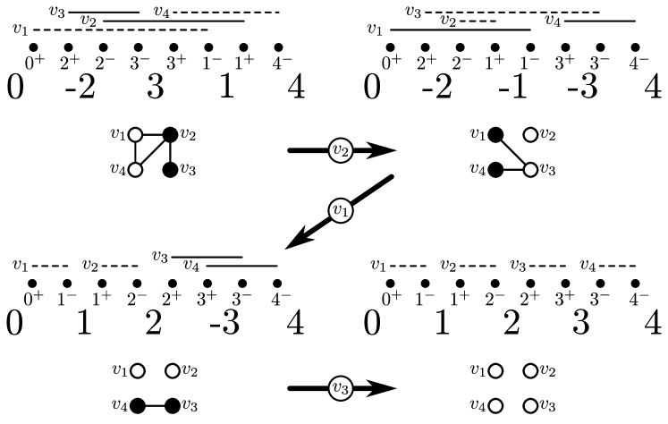
Figure 1: A reversal sequence transforming $(0~{}\raisebox{1.70717pt}{\text{\tiny\boldmath$-$}}2~{}3~{}1~{}4)$ into the identity permutation. At the top, $(0~{}\raisebox{1.70717pt}{\text{\tiny\boldmath$-$}}2~{}3~{}1~{}4)$ is transformed into $(0~{}\raisebox{1.70717pt}{\text{\tiny\boldmath$-$}}2~{}\raisebox{1.70717pt}{\text{\tiny\boldmath$-$}}1~{}\raisebox{1.70717pt}{\text{\tiny\boldmath$-$}}3~{}4)$ by the first reversal $\rho(2,3)=\mu(\raisebox{1.70717pt}{\text{\tiny\boldmath$-$}}2,1)$. The pairs of points for the elements of a permutation appear in a line above the permutation, and an interval for each identity pair is indicated above those points by a black line; lines are solid for good pairs and dashed for bad pairs. The overlap graph for each permutation appears below it; good vertices are colored black and bad are colored white. The sequence of reversals on permutations can be represented by the sequence of vertex complementations indicated by arrows, yielding a graph with only isolated white vertices.

A subpermutation of $\pi$ is an ordered set of consecutive elements in $\pi$. Roughly speaking a framed common interval (FCI) of $\pi$ is a subpermutation that is framed by a smallest integer $a$ and largest integer $b$ while containing a (possibly empty) signed permutation $\pi_{i}~{}\pi_{i+1}\cdots\pi_{j}$ of all integers greater than $a$ and smaller than $b$ [3]. It is “common” with the identity permutation, since it also appears there. Formally, an FCI is a subpermutation $(a~{}\pi_{i}~{}\pi_{i+1}~{}\cdots~{}\pi_{j}~{}b)$ or $(\raisebox{1.70717pt}{\text{\tiny\boldmath$-$}}b~{}\pi_{i}~{}\pi_{i+1}~{}\cdots~{}\pi_{j}~{}\raisebox{1.70717pt}{\text{\tiny\boldmath$-$}}a)$ of $\pi$, such that

1. $a<b$,

2. $(\pi_{i}~{}\pi_{i+1}~{}\cdots~{}\pi_{j})$ is a (possibly empty) signed permutation of the integers $\{a+1,a+2,\dots,b-2,b-1\}$,

3. it is not a union of shorter subpermutations with the first two properties.

Integers $a$ and $b$ are the frame elements and $\{\pi_{i},\pi_{i+1},\ldots,\pi_{j}\}$ are called the internal elements of the FCI. An FCI $B$ is nested in an FCI $A$ if and only if the left and right frame elements of $A$ occur, respectively, before and after the frame elements of $B$. The permutation $\pi$ in Figure 2 has a single FCI, whereas $\pi^{\prime}=(0~{}\raisebox{1.70717pt}{\text{\tiny\boldmath$-$}}5~{}\raisebox{1.70717pt}{\text{\tiny\boldmath$-$}}2~{}\raisebox{1.70717pt}{\text{\tiny\boldmath$-$}}4~{}\raisebox{1.70717pt}{\text{\tiny\boldmath$-$}}3~{}\raisebox{1.70717pt}{\text{\tiny\boldmath$-$}}1~{}6~{}10~{}9~{}7~{}8~{}11)$ has five FCIs, three of which are nested inside at least one other FCI. For example, FCI $(\raisebox{1.70717pt}{\text{\tiny\boldmath$-$}}4~{}\raisebox{1.70717pt}{\text{\tiny\boldmath$-$}}3)$ is nested inside $(\raisebox{1.70717pt}{\text{\tiny\boldmath$-$}}5~{}\raisebox{1.70717pt}{\text{\tiny\boldmath$-$}}2~{}\raisebox{1.70717pt}{\text{\tiny\boldmath$-$}}4~{}\raisebox{1.70717pt}{\text{\tiny\boldmath$-$}}3~{}\raisebox{1.70717pt}{\text{\tiny\boldmath$-$}}1)$, which is in turn nested in $(0~{}\raisebox{1.70717pt}{\text{\tiny\boldmath$-$}}5~{}\raisebox{1.70717pt}{\text{\tiny\boldmath$-$}}2~{}\raisebox{1.70717pt}{\text{\tiny\boldmath$-$}}4~{}\raisebox{1.70717pt}{\text{\tiny\boldmath$-$}}3~{}\raisebox{1.70717pt}{\text{\tiny\boldmath$-$}}1~{}6)$.

A component of $\pi$ is a set containing the frame elements of an FCI along with all internal elements of the FCI that are not an internal element of a nested FCI. As components with less than four elements represent suites of adjacencies, we are interested in non-trivial components with at least four elements. A component is bad if it is non-trivial, and all of its elements have the same sign, otherwise it is good. Note that two components can intersect only at their frame elements. For example, $\pi^{\prime}$ has components $\{\raisebox{1.70717pt}{\text{\tiny\boldmath$-$}}4,\raisebox{1.70717pt}{\text{\tiny\boldmath$-$}}3\}$, $\{\raisebox{1.70717pt}{\text{\tiny\boldmath$-$}}5,\raisebox{1.70717pt}{\text{\tiny\boldmath$-$}}2,\raisebox{1.70717pt}{\text{\tiny\boldmath$-$}}4,\raisebox{1.70717pt}{\text{\tiny\boldmath$-$}}3,\raisebox{1.70717pt}{\text{\tiny\boldmath$-$}}1\}$, $\{0,\raisebox{1.70717pt}{\text{\tiny\boldmath$-$}}5,\raisebox{1.70717pt}{\text{\tiny\boldmath$-$}}1,6\}$, $\{7,8\}$, and $\{6,10,9,7,8,11\}$. Two of the components of $\pi^{\prime}$ are trivial, one is good, and two are bad.

A reversal is called unsafe if it creates a bad component, otherwise it is safe. Reversal $\rho(5,10)$ in Figure 2 is an unsafe reversal on $\pi$, since it creates bad component $\{6,10,9,7,8,11\}$, having elements that are all of the same sign. Working with unsafe reversals is the main obstacle when sorting by reversals, as they must first be detected before being carefully transformed.

1.2 Overview

The task is to construct a minimum length sequence of reversals that sorts a permutation $\pi$. Hannenhalli and Pevzner proved that this can be reduced to the problem of constructing a good sequence of reversals.

Theorem 1 (Hannenhalli and Pevzner [12]).

A reversal sequence $S$ transforming a permutation into the identity is of minimum length if $S$ contains only good reversals.

Each good reversal corresponds to at least one good pair, and it turns out that it is convenient to build a sequence of good pairs, rather than a sequence of reversals. Thus, we refer to good reversals and good pairs synonymously throughout the text.

We work in three domains. Reversals on permutations are related to local complementations of vertex neighborhoods on a particular type of graph. Certain proofs are easier to articulate in this realm, and Algorithm 1 works on graphs but is difficult to make efficient. In order to rapidly compute sequences of good pairs we must operate in the realm of balanced binary search trees. The algorithm presented in Section 5 mimics Algorithm 1, while using the tree as the object to be transformed. The results of Section 4 are most easily stated directly on the permutations themselves.

We assume that $\pi$ does not contain any bad components, since any permutation can be transformed into one without a bad component in linear time, without effecting optimality. Say that $\pi$ contains at least one bad component. There exists a minimum-length sequence $S=S^{\prime}\cdot S^{\prime\prime}$ where $\pi\cdot S$ is the identity permutation, $\pi\cdot S^{\prime}$ has no bad components, and $S^{\prime}$ can be calculated in linear time [1, 3].

The general overview of the algorithm is that we continue building a sequence $S$ of reversals, until there is no good pair in $\pi\cdot S$. At this point, if $\pi\cdot S$ is the identity permutation, then $S$ is of minimum length and we are done. Otherwise, there must have been a bad component created by an unsafe reversal.

If we are stuck without a good pair, we recover by backtracking through reversals until just before the most recent bad reversal, at which point there must exist good pairs in the bad components created by that reversal. With care, some of these good pairs can then be inserted into the sequence; the subsequent reversals that we undid in the backtracking will change, but their corresponding good pairs will not. Section 2 revisits this framework of Tannier et al. [29] by explicitly detailing lemmas that they implicitly used, while adding lemmas that interface more easily with our results. In this section it is most convenient to prove lemmas about vertex complementations on graphs.

Section 3 presents an evolution of the previously used balanced binary search tree from [27], adapted to the recovery scheme. Section 4 proves that the datastructure can perform the backtracking and bad reversal detection efficiently.

While Section 2 presents a new recursive version of the Tannier et al. [29] algorithm along with a proof of correctness, it is not obvious how to directly make this algorithm efficient. Section 5 presents the efficient version of the same algorithm, which operates on the search tree of Section 3, rather than on permutations or on graphs.

In the rest of the section, we finish developing the basic definitions and notions that will be used throughout rest of the article.

1.3 A note on shared notation

In the following section we will define the overlap graph for a permutation, relating vertex complementations on the graph to reversals on permutations. When concepts from the two domains relate to each other, we will share terminology, and sometimes notation. Good and bad pairs in permutations correspond to good (black) and bad (white) vertices in the overlap graph, good and bad components in the permutation correspond to good and bad components in the overlap graph, and good reversals correspond to local complementations of good vertices. An unsafe reversal is, then, a complementation of a good vertex that creates a new all-white component.

The notion of “restriction” will be used for graphs and for permutations alike. In the overlap graph, a restriction is simply an induced subgraph; for a set of vertices $W\subseteq V$ of a graph $H=(V,E)$, the restriction $H[W]$ of $H$ to $W$ is the graph on vertices $W$, having exactly the edges in $E$ with both endpoints in $W$. For a permutation $\pi$ and a set of elements $Q\subseteq\{1,\dots,n\}$, the restriction $\pi[Q]$ of $\pi$ to $Q$ is the permutation $\pi$ with elements not in $Q$ removed. For $\pi$ in Figure 2 and $Q=\{6,7,8,9,10,11\}$, we have $\pi[Q]=(6~{}10~{}9~{}7~{}8~{}11)$.

1.4 The overlap graph

While in Section 4 we work directly on permutations, in the next section the results are most easily articulated in the domain of graphs. Kaplan et al. [14] associated to a permutation $\pi$ a specific type of circle graph [10], called an overlap graph. Roughly speaking, an overlap graph is an intersection graph of the intervals defined by the identity pairs.

Given a permutation $\pi=(0~{}\pi_{1}~{}\cdots~{}\pi_{n}~{}n+1)$, we embed a set of $2n+2$ points on a line, ordered according to the permutation. There is a pair of adjacent points $\pi_{i}^{-}$ and $\pi_{i}^{+}$ for each element $\pi_{i}$, and the points for $\pi_{i}$ come before the points for $\pi_{j}$ if and only if $i<j$. Point $\pi_{i}^{-}$ appears before $\pi_{i}^{+}$ if $\pi_{i}$ is positive, but after it if $\pi_{i}$ is negative. For element $0$ there is the first point $0^{+}$ on the line, and for $n+1$ there is the last point $(n+1)^{-}$. Each pair of points $(q^{+},(q+1)^{-})$ corresponds to an interval on the line. In Figure 1 the points $\{0^{+},1^{-},1^{+},2^{-},2^{+},3^{-},3^{+},4^{-}\}$ are aligned above each of the four genomes. Above the points we have a line for each of the $4$ intervals $(q^{+},(q+1)^{-})$, for $0\leq q<4$.

The overlap graph $OV(\pi)$ for permutation $\pi$ has a vertex for each of the intervals $(q^{+},(q+1)^{-})$, for $0\leq q\leq n$. There is an edge $(u,v)$ if the interval $u$ overlaps with interval $v$, without one interval being contained within the other. A vertex $(q^{+},(q+1)^{-})$ is good if the pair $(q,q+1)$ is good, otherwise it is bad. Below each permutation in Figure 1 appears its overlap graph.

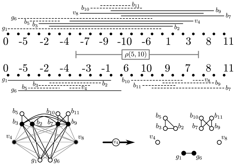
Figure 2: The upper permutation $\pi=(0~{}\raisebox{1.70717pt}{\text{\tiny\boldmath$-$}}5~{}\raisebox{1.70717pt}{\text{\tiny\boldmath$-$}}2~{}\raisebox{1.70717pt}{\text{\tiny\boldmath$-$}}4~{}\raisebox{1.70717pt}{\text{\tiny\boldmath$-$}}7~{}\raisebox{1.70717pt}{\text{\tiny\boldmath$-$}}9~{}\raisebox{1.70717pt}{\text{\tiny\boldmath$-$}}10~{}\raisebox{1.70717pt}{\text{\tiny\boldmath$-$}}6~{}1~{}3~{}8~{}11)$ is transformed into $\pi^{\prime}=\pi\rho(5,10)=(0~{}\raisebox{1.70717pt}{\text{\tiny\boldmath$-$}}5~{}\raisebox{1.70717pt}{\text{\tiny\boldmath$-$}}2~{}\raisebox{1.70717pt}{\text{\tiny\boldmath$-$}}4~{}\raisebox{1.70717pt}{\text{\tiny\boldmath$-$}}3~{}\raisebox{1.70717pt}{\text{\tiny\boldmath$-$}}1~{}6~{}10~{}9~{}7~{}8~{}11)$ through the unsafe reversal $\rho(5,10)=\mu(3,\raisebox{1.70717pt}{\text{\tiny\boldmath$-$}}4)=\mu(\raisebox{1.70717pt}{\text{\tiny\boldmath$-$}}7,8)$. The overlap graph for $\pi$ is on the bottom-left, and the overlap graph for $\pi^{\prime}$ is on the bottom-right. Vertices from the bad components of $OV(\pi^{\prime})$ are labeled by $b$ and vertices from the good components are labeled by $g$. See the caption of Figure 1 for a more detailed description.

The overlap graph construction implicates a bijection between the components of a permutation $\pi$ and the connected components of $OV(\pi)$ [3]. Reversals on permutations, then, correspond to an operation called a local complementation of a vertex in the graph.

The local complementation operation is defined on a graph $H=(V,E)$, where each vertex is colored either black or white, corresponding in our case to a vertex that is good or bad, respectively. The neighborhood of a vertex $v\in V$, denoted $N(v)$, is the set of vertices adjacent to $v$ in $H$.

Definition.

The local complementation of a good vertex $v\in V$, denoted $H/v$, complements the neighborhood $W=N(v)\cup\{v\}$, while toggling all vertices in $W$ from good to bad, or vice versa. That is, there is an edge $e$ in $H/v$ if and only if $e$ is not in $H[W]$ or $e$ is in $H[V\setminus W]$.

Note, then, that $v$ is always isolated and bad in $H/v$.

The task of sorting by reversal can be reduced to that of “sorting” a graph, by finding a sequence of complementations of good vertices $v_{1}v_{2}\cdots v_{m}$ that yields only isolated vertices in $H/v_{1}v_{2}\cdots v_{m}$.

2 Tannier, Bergeron, and Sagot’s approach

The main contribution of Tannier et al. [29] was a clever technique for recovering from an unsafe reversal. They construct a sequence of reversals $S=\rho_{1}\rho_{2}\ldots\rho_{m}$ by always choosing a good reversal as long as one exists, knowing that the absence of such a reversal implies that either the permutation is sorted, or that an unsafe reversal exists somewhere in $S$. The key observation they make is that all of the reversals after the most recent unsafe reversal $\rho_{i}$ can be applied at the end of the sorting sequence, when the proper precautions are made. To that end, they presented the following theorem.

Theorem 2 (Tannier et al. [29]).

For any sequence $S$ of good reversals such that $\pi\cdot S$ has all positive elements, there exists a nonempty reversal sequence $S^{\prime}$ such that $S$ can be split into two $S=S_{1}\cdot S_{2}$, and $S_{1}\cdot S^{\prime}\cdot S_{2}$ is a good sequence on $\pi$.

While the algorithm that they developed is inspired by this theorem, some of the elements of the algorithm’s correctness are hidden in the proof of the theorem, and some are left implicit, making it difficult for us to use their results directly. Therefore, in this section we motivate a new recursive variant of the algorithm, while providing a thorough proof of correctness. The general structure of these results is then used in our algorithm presented in Section 5.

2.1 Sorting by complementation

In [29], Theorem 2 is actually stated in a more general form that applies to local complementations on a bi-colored graph. Their approach is based on the observation that an overlap graph has a particular structure, just before a bad component is created by an unsafe complementation of a vertex $v$. Due to this structure, the complementation of $v$ can be made safe by inserting vertices before it in the already computed complementation sequence.

We first outline the structure in two remarks, before exploring the consequences. The general idea is to focus on the state of a graph just before an unsafe complementation. In this section, we will call a graph in this state $H$, and the unsafe complementation $v$. The vertices of $H$ can be partitioned into the set $B$ containing the bad components of $H/v$, and the set $G$ containing the good components. We show that the sequence of vertices that sorts the induced subgraph $H[B]$ can always be done before the sequence of vertices that sorts $H[G]$. This allows us to iteratively proceed until we get stuck, having no good vertices to act on, before “recovering” by undoing the sequence on $H[G]$ and inserting a new sequence on $H[B]$ before $v$.

The following remark is a simple consequence of the definition of local vertex complementation. See Figure 3 for an illustration.

Remark 1.

The complementation of a vertex $v$ will split a single component into $\ell$ new components $C_{1},C_{2},\ldots,C_{\ell}$ if and only if for all $1\leq i<j\leq\ell$

1. there are all possible edges between $C_{i}\cap N(v)$ and $C_{j}\cap N(v)$, and

2. there is no edge between $C_{i}\setminus N(v)$ and $C_{j}\setminus N(v)$.

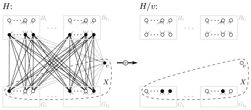
Figure 3: On the left, a graph $H$ has a single connected component, before being split into graph $H/v$ having bad components $B_{1},B_{2},\ldots,B_{\ell_{1}}$ and good components $G_{1},G_{2},\ldots,G_{\ell_{2}}$, on the right. Good vertices are filled in black. Note that, due to the definition of vertex complementation, all vertices from $B=\cup_{i=1}^{\ell_{1}}B_{i}$ that are adjacent to $v$ must be good, while the others from $B$ must be bad. If, instead of $v$, a good vertex $u$ from $B$ is applied to $H$, then any good vertex in $H/u[B]$ will be adjacent to all the vertices of $X$.

Consider a graph $H$ with a single connected component, where the complementation of vertex $v$ creates the graph $H/v$ with bad components $B_{1},B_{2},\ldots,B_{\ell_{1}}$ and good components $G_{1},G_{2},\ldots,G_{\ell_{2}}$. Call $B=\cup_{i=1}^{\ell_{1}}B_{i}$ the set of vertices that are in bad components of $H/v$, and $G=\cup_{i=1}^{\ell_{2}}G_{i}$ the set of vertices that are in good components of $H/v$. The properties of Remark 1 impose strong constraints on the colors of vertices in $B$, just before the unsafe complementation of vertex $v$ in $H$ (see Figure 3).

Remark 2.

All vertices from $B$ that are adjacent to $v$ in $H$ are good, while the other vertices from $B$ are bad.

The following lemma guarantees that, if instead of complementing $v$, we choose a vertex $u$ from $B$ to complement, we are guaranteed to have additional good vertices in $B$. This is useful since it means we can build a complementation sequence of at least two good vertices, when recovering from the unsafe complementation of $v$.

Lemma 1.

For any good vertex $u\in B$ in $H$, there exists at least one good vertex in $H/u[B]$.

Proof.

If $u$ is adjacent to a bad vertex in $H[B]$, then the lemma is clearly true. If $u$ is not adjacent to a bad vertex in $H[B]$, then there must exist some other vertex $u^{\prime}\in B$ that is adjacent to $u$ in $H/v[B]$, otherwise $u$ would be isolated in $H/v[B]$, contradicting its membership in $B$. Vertex $u^{\prime}$, then, is not adjacent to $u$ in $H$ and is good in $H/u$. ∎

The following lemmas delineate the pertinent properties of the vertices that are adjacent to every member of $B\cap N(v)$ in $H$. Call these vertices $X=(G\cap N(v))\cup\{v\}$, as indicated in Figure 3. The objective is to eventually show that any vertex sequence sorting the components of $B$ can be placed before any vertex sequence sorting the components of $G$.

Lemma 2.

Consider a good vertex sequence $v_{1}v_{2}\cdots v_{m}$ on $H$, composed from a subset of vertices in $B$. Any good vertex in $H/v_{1}\cdots v_{m}[B]$, has each of the vertices of $X$ in its neighborhood, and none of the vertices of $G\setminus X$.

Proof.

Remarks 1 and 2 demonstrate that the statement is true in $H$ (when $m=0$). Say the property holds for $H/v_{1}\cdots v_{i-1}$. Then when we complement good vertex $v_{i}$, any good neighbor of $v_{i}$ will become disconnected from the vertices of $X$ and bad, while any bad neighbor of $v_{i}$ will become connected to $X$ and good. ∎

The following is a corollary of Lemma 2 and Remark 1.2, as each complementation in $v_{1}v_{2}\cdots v_{m}$ will complement connectivity in $X$ while leaving the rest of $G$ unchanged.

Corollary 1.

Consider a good vertex sequence $v_{1}v_{2}\cdots v_{m}$ on $H$ of even length, composed from a subset of vertices in $B$. Then $H/v_{1}\cdots v_{m}[G\cup\{v\}]=H[G\cup\{v\}]$.

Lemma 3.

Consider a good vertex sequence $v_{1}v_{2}\cdots v_{m}$, composed from a subset of vertices in $B$, such that $H/v_{1}\cdots v_{m}[B]$ has no good vertex. If $m$ is even then $H/v[G\cup\{v\}]=H/v_{1}\cdots v_{m}v[G\cup\{v\}]$, otherwise $H/v[G\cup\{v\}]=H/v_{1}\cdots v_{m}[G\cup\{v\}]$ if $m$ is odd.

Proof.

When the length $m$ of the sequence is even, Corollary 1 implies that $v$ is good in $H/v_{1}\cdots v_{m}[G\cup\{v\}]$, and that $H/v[G\cup\{v\}]=H/v_{1}\cdots v_{m}v[G\cup\{v\}]$.

If $m$ is odd, then $H[G\cup\{v\}]=H/v_{1}\cdots v_{m-1}[G\cup\{v\}]$ by Corollary 1. Since $v_{m}$ is good in $H/v_{1}\cdots v_{m-1}$, Lemma 2 implies that $v_{m}$ has exactly the vertices of $X$ in its neighborhood in $H/v_{1}\cdots v_{m-1}$. By the definition of $v$, it is adjacent to vertices $\{v_{m}\}\cup X\setminus\{v\}$ in $H[G]$. Thus, the same adjacencies are complemented by $v$ in $H[G\cup\{v\}]$ as are complemented by $v_{m}$ in $H/v_{1}\cdots v_{m-1}[G\cup\{v\}]$, and we have $H/v[G\cup\{v\}]=H/v_{1}\cdots v_{m}[G\cup\{v\}]$. ∎

2.2 Sorting overlap graphs

Lemma 3 inspires the following recursive algorithm for sorting an overlap graph with good components.

Algorithm 1 Sort a good component by vertex complementation.

$\triangleright$ Compute sorting sequence for good components of $H[Q]$.

procedure SortGraph($H,Q$)

     $S_{f},Q$ $\leftarrow$ DoGood($H,Q$)

     $S_{b}$ is an empty sequence $\triangleright$ $f$ for “front” and $b$ for “back”

     while $S_{f}$ is not empty do

         $S_{1},S_{2}$ $\leftarrow$ Recover($H,S_{f},Q$) $\triangleright$ $S_{1}\cdot S_{2}=S_{f}$

         $S^{\prime},Q$ $\leftarrow$ SortGraph($H/S_{1},Q$)

         if $even(|S^{\prime}|)$ then

              $S_{b}$ $\leftarrow$ $S^{\prime}\cdot S_{2}\cdot S_{b}$

         else

              $S_{b}$ $\leftarrow$ $S^{\prime}\cdot S_{2}^{-}\cdot S_{b}$ $\triangleright$ $S_{2}^{-}$ is $S_{2}$ without the first vertex          

         $S_{f}$ $\leftarrow$ $S_{1}$      

     return $S_{b},Q$

$\triangleright$ Complement good vertices in $H[Q]$ until there are none.

procedure DoGood($H,Q$)

     $S$ is an empty sequence

     while $H/S[Q]$ has a good vertex do

         $v$ $\leftarrow$ GetGood($H/S[Q]$) $\triangleright$ any good vertex in $H/S[Q]$

         $Q$ $\leftarrow$ $Q\setminus\textsc{Isolated}(H/Sv[Q])$ $\triangleright$ remove newly isolated vertices

         $S$ $\leftarrow$ $Sv$      

     return $S,Q$

$\triangleright$ Get largest prefix $S_{1}$ of $S$ such that $H/S_{1}[Q]$ has a good vertex.

procedure Recover($H,S,Q$)

     $S_{2}$ is an empty sequence $\triangleright$ $S_{1}\cdot S_{2}=S$

     $S_{1}$ $\leftarrow$ S

     while $S_{1}$ is nonempty and $H/S_{1}[Q]$ has no good vertex do

         $v$ $\leftarrow$ $pop(S_{1})$ $\triangleright$ $pop()$ removes $v$ from the end

         $S_{2}$ $\leftarrow$ $v\cdot S_{2}$      

     return $S_{1},S_{2}$

In the following, we show that Algorithm 1 builds a sequence of good vertices, which is guaranteed to be of minimum length due to Theorem 1.

Focus first on the $H$ and $Q$ within DoGood. Clearly, DoGood returns a sequence $S$ of good vertices on $H[Q]$, and the $Q$ that is returned contains only vertices that are bad and unisolated in $H/S[Q]$.

Now focus on the $H$, $S$, and $Q$ within Recover. Clearly, Recover returns the $S_{1}$ and $S_{2}$ such that $S=S_{1}\cdot S_{2}$, the graph $H/S_{1}[Q]$ has a good vertex, and $S_{2}$ is of minimum length.

We now argue that a call to SortGraph($H,Q$) computes a sorting sequence for $H[Q]$. Sequence $S_{f}$ is first build from good vertices in $H$. The while loop iteratively backtracks through $S_{f}$ using calls to Recover; suffixes of $S_{f}$ are moved to $S_{b}$.

If $S_{1}$ is not empty after a call to Recover, this indicates that there were bad components $B_{1},B_{2},\dots,B_{\ell_{1}}$ in $H/S_{f}[Q]$. According to Remark 2, the graph $H/S_{1}[Q]$ has good vertices, which come from the bad components that we will call $B_{1},\dots,B_{k}$, for $1\leq k\leq\ell_{1}$. Lemma 3 ensures that, after the recursive call to SortGraph($H/S_{1},Q$), the sequence $S^{\prime}$ that sorts components $B_{1},\dots,B_{k}$ can safely be inserted between $S_{1}$ and $S_{2}$.

At the end of an iteration of the while loop, there are no good vertices; this is obviously true when $|S^{\prime}|$ is even, but is also true when $|S^{\prime}|$ is odd due to similar reasoning as the proof of Lemma 3 (i.e. complementation of the final vertex of $S^{\prime}$ has the same effect on the graph as complementation of the first vertex of $S_{2}$). The next iteration backtracks to find another vertex complementation that created some bad components, and when $S_{f}$ is empty, $Q$ is also empty and the graph $H$ has no remaining nontrivial components. Each call to SortGraph is independent from the previous, since each of them works on a disjoint subset of the bad components $B_{1},\dots,B_{\ell_{1}}$.

The recursive call to SortGraph is performed at most $n$ times, since by Lemma 1 it will return a sequence with at least two vertices, and since each of the calls to SortGraph works on an independent set of good components from the previous calls. The running time of the algorithm, therefore, depends on the cost of the GetGood call, the cost of doing or undoing a vertex complementation on the graph, and the cost of removing a vertex from $Q$; it is clear that each of these are done at most once for each vertex in the graph.

In the following sections we present a datastructure, along with the other necessary formalities, showing that each these steps can be performed in $O(\log n)$ amortized time.

3 Maximum and minimum pairs

Previous approaches maintained datastructures containing the complete complement of good pairs which, as yet, has made it difficult to obtain an $O(n\log n)$ running time. In [27], however, we ensured that we could always efficiently retrieve two specific good pairs of $\pi$: the pair that contains the maximum negative integer $\mathsf{M}^{-}(\pi)$, and the pair that contains the minimum negative integer $\mathsf{m}^{-}(\pi)$. In Figure 2 we have $\mathsf{M}^{-}(\pi)=2$, $\mathsf{m}^{-}(\pi)=10$, $\mathsf{M}^{-}(\pi^{\prime})=1$, and $\mathsf{m}^{-}(\pi^{\prime})=5$.

Since sorting by reversals is an iterative process, it is natural to speak in reference to an implied “current” permutation. When it is clear from the context, we will drop the $\pi$ and just speak of the (“maximum negative”) $\mathsf{M}^{-}$ element in the current permutation, along with its $\mathsf{M}^{-}$ pair.

The use of $\mathsf{M}^{-}$ and $\mathsf{m}^{-}$ pairs in [27] enabled us to find a good reversal in logarithmic time, yet had the drawback of requiring convoluted and inefficient recovery steps when no good reversal remained. In this section we supplement the datastructure with subsets of the unsigned integers in $\pi$ that are still “eligible” to be a maximum/minimum negative element in a good pair, ensuring that, when recovering we can ignore pairs that have already been repaired by a reversal. Call $Q_{\mathsf{M}}$ the set containing every element $q\in\{1,\dots,n+1\}$ such that the adjacency ($(q-1)$ $q$) does not exist in the current permutation, and call $Q_{\mathsf{m}}$ the set of elements containing $q\in\{0,\dots,n\}$, such that the adjacency ($q$ $(q+1)$) does not exist. Thus, any possible good pair $(\pi_{i},\pi_{j})$ that does not yet form an adjacency, is represented by one element of $Q_{\mathsf{M}}$ and one element of $Q_{\mathsf{m}}$. For example when $|\pi_{i}|<|\pi_{j}|$ we have $|\pi_{i}|\in Q_{\mathsf{m}}$ and $|\pi_{j}|\in Q_{\mathsf{M}}$.

Maintaining these sets allows us to use simpler recovery steps within the framework of a modified version of the Tannier et al. [29] algorithm; we prove in the next section that during recovery either the $\mathsf{M}^{-}$ element must be in $Q_{\mathsf{M}}$, or the $\mathsf{m}^{-}$ element must be in $Q_{\mathsf{m}}$. To simplify the exposition we use a splay tree, but other balanced binary search trees based on rotations (e.g. AVL trees and Red-black trees) could be used to similar effect, thereby avoiding amortized running times.

3.1 The datastructure

Consider an ordered binary tree where each node $v$ represents an element $\pi_{i}$ of a signed permutation $\pi$, noting that throughout this section we will refer to $v$ and $\pi_{i}$ interchangeably. The initial conditions of the tree ensure that an in-order traversal visits vertices in the order that the elements appear in the permutation. Thus, each subtree represents a subset of contiguous elements of $\pi$.

Along with subtree size, we associate to each node several values specific to our application. The extremal values for the subtree rooted at $v$ are the

• $\mathsf{M}^{-}(v)$ and $\mathsf{M}^{+}(v)$ integers equal to the maximum negative/positive elements from $Q_{\mathsf{M}}$ that appear in the subtree rooted at $v$, set to $\raisebox{1.70717pt}{\text{\tiny\boldmath$-$}}\infty$/zero if none exist, and the

• $\mathsf{m}^{-}(v)$ and $\mathsf{m}^{+}(v)$ integers equal to the minimum negative/positive elements from $Q_{\mathsf{m}}$ that appear in the subtree rooted at $v$, set to zero/$\infty$ if none exist.

A $rev(v)$ boolean flag indicates the subtree rooted at $v$ is in reverse order. The $Q$ membership values for a vertex $v$ are the

• $inQ_{\mathsf{M}}(v)$ boolean flag to indicate the element at $v$ is in $Q_{\mathsf{M}}$, and the

• $inQ_{\mathsf{m}}(v)$ boolean flag to indicate the element at $v$ is in $Q_{\mathsf{m}}$.

Note that a node $v$ has an implicit parity based on the number of $rev$ flags on the path from $v$ to the root. Say that the left child of $v$ is the first child of $v$, and that the right child is the last child, if the parity of $v$ is even. Otherwise, the right child is the first, and the left child is the last. An in-order traversal of a tree, then, recursively visits before $v$ all nodes in the subtree rooted at the first child, and visits after $v$ all nodes in the subtree rooted at the last child. Before any reversals have been done, the parity of every vertex is even since all $rev$ flags are initialized to false.

Similar to the in-order traversal we just described, the $rev$ flags act on the extremal values. Since reversals flip the signs of the elements that are reversed, the maximum negative element from $Q_{\mathsf{M}}$ in the subtree rooted at $v$ is $\mathsf{M}^{-}(v)$ if the parity of $v$ is even, and $\mathsf{M}^{+}(v)$ otherwise.

Definition.

Call $\mathcal{T}(\pi,Q)$ the set of ordered trees, for a signed permutation $\pi$ and integer subsets $(Q_{\mathsf{M}},Q_{\mathsf{m}})=Q$, such that any tree $T\in\mathcal{T}(\pi,Q)$ has the following properties:

1. $\pi$ can be retrieved by an in-order traversal of $T$, and

2. extremal values $\mathsf{M}^{-}(v)$ and $\mathsf{m}^{-}(v)$ can be retrieved by traversing $T$ from the root to any node $v$.

Figure 4 shows splay trees for $\pi$ and $\pi^{\prime}$ from Figure 2.

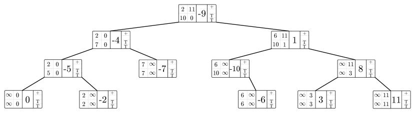
(a) A tree from $\mathcal{T}(\pi,Q)$ where $\pi=(0~{}\raisebox{1.70717pt}{\text{\tiny\boldmath$-$}}5~{}\raisebox{1.70717pt}{\text{\tiny\boldmath$-$}}2~{}\raisebox{1.70717pt}{\text{\tiny\boldmath$-$}}4~{}\raisebox{1.70717pt}{\text{\tiny\boldmath$-$}}7~{}\raisebox{1.70717pt}{\text{\tiny\boldmath$-$}}9~{}\raisebox{1.70717pt}{\text{\tiny\boldmath$-$}}10~{}\raisebox{1.70717pt}{\text{\tiny\boldmath$-$}}6~{}1~{}3~{}8~{}11)$, and $Q=(\{0,\dots,11\},\{0,\dots,11\})$.

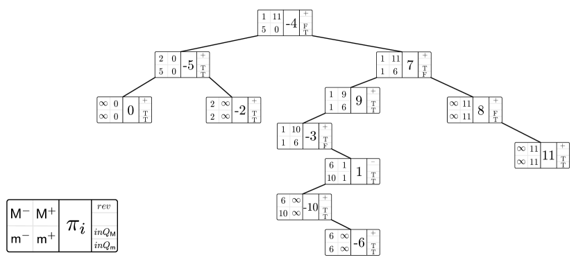
(b) A tree from $\mathcal{T}(\pi^{\prime},Q^{\prime})$ where $\pi^{\prime}=\pi\mu(\raisebox{1.70717pt}{\text{\tiny\boldmath$-$}}7,8)=(0~{}\raisebox{1.70717pt}{\text{\tiny\boldmath$-$}}5~{}\raisebox{1.70717pt}{\text{\tiny\boldmath$-$}}2~{}\raisebox{1.70717pt}{\text{\tiny\boldmath$-$}}4~{}\raisebox{1.70717pt}{\text{\tiny\boldmath$-$}}3~{}\raisebox{1.70717pt}{\text{\tiny\boldmath$-$}}1~{}6~{}10~{}9~{}7~{}8~{}11)$, and $Q^{\prime}=(\{0,1,2,3,5,6,7,9,10,11\},\{0,1,2,4,5,6,8,9,10,11\})$. Note that the $rev$ flag in the node for element $1$ is set to true, indicated by the ‘$-$’ in its corner.

Figure 4: A splay tree a) before, and b) after the reversal $\mu(\raisebox{1.70717pt}{\text{\tiny\boldmath$-$}}7,8)$ of Figure 2. Nodes are labeled by the values indicated in the bottom-left corner of the figure.

3.2 Reversals on trees

The operation $splay(\pi_{i})$, on a tree $T\in\mathcal{T}(\pi,Q)$, moves the non-root vertex $\pi_{i}$ to the root, producing a new tree in $\mathcal{T}(\pi,Q)$ having the $rev$ flag at the root set to false. A splay is done through a series of rotate operations, which are carefully chosen to make the tree self-balancing, so that $n$ splays will take $O(n\log n)$ time to perform [21]. Consider a node $x$ with parent $y$, as depicted in the left panel of Figure 5.

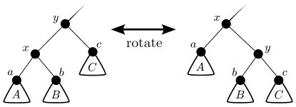
Figure 5: A rotation promotes a node above its parent, while keeping the in-order traversal intact.

The $rotate(x)$ operation promotes $x$ above its parent, while maintaining the order of the nodes visited by an in-order traversal.

The skeleton of the following lemma was implicit in our previous work, which we augment with information related to $Q=(Q_{\mathsf{M}},Q_{\mathsf{m}})$.

Lemma 4.

A rotate operation can be performed on a tree from $\mathcal{T}(\pi,Q)$ in constant time, yielding another tree from $\mathcal{T}(\pi,Q)$.

Proof.

Without loss of generality, consider the $rotate(x)$ operation on the subtree in the left panel of Figure 5, creating the subtree in the right panel.

Before performing $rotate(x)$, we ensure that nodes $x$ and $y$ do not have $rev$ flags set to true. If $rev(y)=\texttt{true}$, we swap the order of children $x$ and $c$ while flipping the $rev(x)$ and $rev(c)$ values, and then we swap $\mathsf{M}^{-}(y)$ with $\mathsf{m}^{+}(y)$ and swap $\mathsf{m}^{-}(y)$ with $\mathsf{M}^{+}(y)$. The product of this transformation is a tree in $\mathcal{T}(\pi,Q)$ since, while there is one fewer $rev$ flag from $y$ to the root, the order of the children have been swapped, along with the extremal values. Further, the parity of $x$ (and $c$) is even after the modification, if and only if the parity of $x$ (and $c$) was even before the modification. If $rev(x)=\texttt{true}$, then do the analogous modifications to node $x$ and its children, yielding another tree in $\mathcal{T}(\pi,Q)$.

Now we perform the rotate operation on a tree with $rev(x)$ and $rev(y)$ set to false by removing two edges and adding two edges, as depicted in Figure 5. Note that the only extremal values that will change during this rotation are the values at nodes $x$ and $y$. We set

$$\mathsf{M}^{-}(y)=\begin{cases}\max(\mathsf{M}^{-}(b),\mathsf{M}^{-}(c),y)&\text{if }y<0\land inQ_{\mathsf{M}}(|y|),\\ \max(\mathsf{M}^{-}(b),\mathsf{M}^{-}(c))&\text{otherwise}.\end{cases}$$

The other extremal values for nodes $y$ and $x$ are updated in similar ways. ∎

Kaplan and Verbin [13] noticed that the datastructure used by Chrobak et al. [8] to reverse suffixes of travelling salesman paths could be easily adapted to reversals on permutations, by using a sequence of splay operations. Lemma 4 assures us that these splay operations produce a tree from the same set. Splitting and joining splay trees at their roots are efficient for similar reasons as the rotate operation.

Remark 3 (Kaplan and Verbin [13]).

A series of splay operations can update a tree $T\in\mathcal{T}(\pi,Q)$ through a reversal $\rho(i,j)$ to obtain a tree in $\mathcal{T}(\pi\rho(i,j),Q)$, in (amortized) logarithmic time.

The process works in five steps. First we

1. $splay(\pi_{i-1})$ and split the right child from the root, yielding trees $T_{<i}$ and $T_{\geq i}$ (i.e. $T_{<i}$ contains the elements in $\pi_{0}\,\,\pi_{1}\,\cdots\,\pi_{i-1}$),

2. $splay(\pi_{j})$ in $T_{\geq i}$ and split the right child from the root, yielding trees $T_{i..j}$ and $T_{>j}$ (i.e. $T_{>j}$ contains the elements in $\pi_{j+1}\,\pi_{j+2}\,\cdots\,\pi_{n+1}$),

3. set the $rev$ flag at the root of $T_{i..j}$,

4. $splay(last(T_{i..j}))$ so that there is no right child of the root, and join $T_{>j}$ as the right child to create $T_{\geq i}^{\prime}$,

5. join $T_{\geq i}^{\prime}$ as the right child of the root of $T_{<i}$,

where $last(T_{i..j})$ is the node corresponding to the last element in the permutation represented by $T_{i..j}$. For an example see Figure 6, which describes the intermediate states between the trees from Figure 4 during the reversal process.

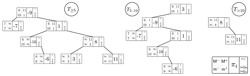
Figure 6: Subtrees created during the process of the reversal $\mu(\raisebox{1.70717pt}{\text{\tiny\boldmath$-$}}7,8)=\rho(5,10)$ on the tree from Figure 4(a), eventually resulting in the tree of Figure 4(b). $T_{\geq 5}$ is the right subtree of the root, after $splay(\raisebox{1.70717pt}{\text{\tiny\boldmath$-$}}4)$ is done on the tree of Figure 4(a). $T_{5..10}$ is then obtained from $T_{\geq 5}$ by doing $splay(3)$ and then splitting the right child of the root $T_{>10}$. The tree of Figure 4(b) is obtained by doing $splay(7)$ on $T_{5..10}$ before joining the trees back together.

Note that, in order to make a reversal efficient, we maintain a vector of pointers from elements to their corresponding nodes. Thus, for a good pair $(\pi_{i},\pi_{j})$, the node $\pi_{i}$ can be accessed using the vector, even when the index $i$ is not known. To access $\pi_{i-1}$, the position $i$ can be found using the node $\pi_{i}$ in the search tree, before re-descending from the root to find the element at position $i-1$. When performing a reversal for a good pair, we remove the appropriate values from $Q_{\mathsf{M}}$ and $Q_{\mathsf{m}}$, thereby ignoring the corresponding breakpoints when choosing future good pairs.

Theorem 3.

Reversal $\mu(\pi_{i},\pi_{j})$ can be performed on a tree from $\mathcal{T}(\pi,Q)$, producing a tree from $\mathcal{T}(\pi\mu(\pi_{i},\pi_{j}),Q^{\prime})$ in (amortized) logarithmic time, where

$$Q^{\prime}=\big{(} Q_{\mathsf{M}}\setminus\{\max(|\pi_{i}|,|\pi_{j}|)\},$$

$$Q_{\mathsf{m}}\setminus\{\min(|\pi_{i}|,|\pi_{j}|)\}\big{)}$$

Proof.

First, note that the extremal values are trivial to maintain when a tree is split at the root, and when trees are joined by making one root the child of the other.

Say $\pi_{i}$ is negative. After the first splay of Remark 3, $\pi_{i}$ is the root, and we mark $inQ_{\mathsf{M}}(\pi_{i})=\texttt{false}$ when $|\pi_{i}|>|\pi_{j}|$ and $inQ_{\mathsf{m}}(\pi_{i})=\texttt{false}$ otherwise, before updating the extremal values at the root in the obvious way. After the second splay we mark $inQ_{\mathsf{M}}(\pi_{j})=\texttt{false}$ when $|\pi_{i}|<|\pi_{j}|$ and $inQ_{\mathsf{m}}(\pi_{j})=\texttt{false}$ otherwise, and then we update the extremal values at the root in the obvious way. Lemma 4 ensures that $T_{i..j}$ is now a tree from $\mathcal{T}((\pi_{i}~{}\pi_{i+1}~{}\cdots~{}\pi_{j}),Q^{\prime})$, and that the subsequent splaying and joining of trees yields a tree in $\mathcal{T}(\pi\mu(\pi_{i},\pi_{j}),Q^{\prime})$.

A similar argument applies to the symmetric case of a negative $\pi_{j}$. ∎

4 Recovery

Recall from Section 2 that when we get stuck at a permutation $\pi\cdot S$ having only positive elements, we backtrack until we find the most recent unsafe reversal $\rho_{k}$. This partitions the sequence $S$ into $S_{1}=\rho_{1}\cdots\rho_{k-1}$ and $S_{2}=\rho_{k}\cdots\rho_{|S|}$. Also recall from Section 3 that, after performing a $\mathsf{M}^{-}$ reversal, which creates an adjacency ($q$ $(q+1)$) (or equivalently ($\raisebox{1.70717pt}{\text{\tiny\boldmath$-$}}(q+1)$ $\raisebox{1.70717pt}{\text{\tiny\boldmath$-$}}q$)), we are guaranteed that $\raisebox{1.70717pt}{\text{\tiny\boldmath$-$}}(q+1)$ will never be the $\mathsf{M}^{-}$ element and $\raisebox{1.70717pt}{\text{\tiny\boldmath$-$}}q$ will never be the $\mathsf{m}^{-}$ element in later sorting steps, so we remove $q+1$ from $Q_{\mathsf{M}}$ and $q$ from $Q_{\mathsf{m}}$. In this section, we motivate an efficient strategy for finding $\rho_{k}$, based on undoing reversals from $S$ until certain conditions appear on the eligible negative elements of a permutation.

When we get stuck at a permutation with all positive elements, there exist bad non-trivial components $B_{1},B_{2},\ldots,B_{\ell}$ with internal elements $I=\cup_{i=1}^{\ell}I_{i}$ framed by smallest elements $A=\cup_{i=1}^{\ell}a_{i}$ and greatest elements $B=\cup_{i=1}^{\ell}b_{i}$. At this point, sets $Q_{\mathsf{M}}$ and $Q_{\mathsf{m}}$ are related to these components in the following ways:

1. $Q_{\mathsf{M}}=I\cup B$, and

2. $Q_{\mathsf{m}}=I\cup A$.

For example, say we continue sorting the $\pi$ of Figure 2 by doing the reversals on $\pi^{\prime}$ that sort the component $\{0,\raisebox{1.70717pt}{\text{\tiny\boldmath$-$}}5,\raisebox{1.70717pt}{\text{\tiny\boldmath$-$}}2,\raisebox{1.70717pt}{\text{\tiny\boldmath$-$}}4,\raisebox{1.70717pt}{\text{\tiny\boldmath$-$}}3,\raisebox{1.70717pt}{\text{\tiny\boldmath$-$}}1,6\}$. The remaining bad component is $\{6,10,9,7,8,11\}$, with frame elements $6$ and $11$, implying $Q_{\mathsf{M}}=\{10,9,7,8,11\}$ and $Q_{\mathsf{m}}=\{6,10,9,7,8\}$.

Denote $p_{0}=\pi$, and the permutations visited in sequence $S$ as $p_{j}=p_{j-1}\rho_{j}$, for $1\leq j\leq|S|$, so that $p_{k}$ is the first permutation after the most recent unsafe reversal $\rho_{k}$ (i.e. $k$ is maximum such that $\rho_{k}$ is unsafe).

The following results concern the states of $Q_{\mathsf{M}}$ and $Q_{\mathsf{m}}$ that exist after applying $S$ to $\pi$. We call these sets $Q_{\mathsf{M}}^{S}$ and $Q_{\mathsf{m}}^{S}$. Lemma 5 establishes an easy way to check that all of the bad components remain intact, when backtracking through the permutations $p_{|S|},p_{|S|-1},\dots,p_{k}$. Lemma 6 states that one element from the bad components of $\pi\cdot S$ must be negative in $p_{k-1}=\pi\cdot S_{1}$, while Lemma 7 ensures that we can find a good pair by looking at the $\mathsf{M}^{-}$ and $\mathsf{m}^{-}$ elements of the permutation $\pi\cdot S_{1}[Q_{\mathsf{M}}^{S}\cup Q_{\mathsf{m}}^{S}]$.

Lemma 5.

Consider a permutation $p_{j}$ for $k\leq j\leq|S|$. It either has no elements from $Q_{\mathsf{M}}^{S}$ that are negative, or $q-1$ is negative in $p_{j}$ when $\raisebox{1.70717pt}{\text{\tiny\boldmath$-$}}q$ is the $\mathsf{M}^{-}$ element in $p_{j}[Q_{\mathsf{M}}^{S}]$. Symmetrically, $p_{j}$ either has no elements from $Q_{\mathsf{m}}^{S}$ that are negative, or $q+1$ is also negative in $p_{j}$ when $\raisebox{1.70717pt}{\text{\tiny\boldmath$-$}}q$ is the $\mathsf{m}^{-}$ element in $p_{j}[Q_{\mathsf{m}}^{S}]$.

Proof.

By definition, $Q_{\mathsf{M}}^{S}$ contains all elements from each bad component in $\pi\cdot S$ except for the one in each component with smallest absolute value. So if there is a $\mathsf{M}^{-}$ element $\raisebox{1.70717pt}{\text{\tiny\boldmath$-$}}q$ in $p_{j}[Q_{\mathsf{M}}^{S}]$, then the smallest element of the component is $q-1$. Since $\rho_{k}$ is the most recent unsafe reversal, any bad component in $p_{|S|}$ is bad in $p_{j}$, and all elements of such a component have the same sign, including element $q-1$. By symmetry, the same is true for the $\mathsf{m}^{-}$ element and $Q_{\mathsf{m}}^{S}$. ∎

Lemma 6.

There is at least one element from $Q_{\mathsf{M}}^{S}\cup Q_{\mathsf{m}}^{S}$ that is negative in the permutation $\pi\cdot S_{1}=p_{k-1}=p_{k}\rho_{k}$.

Proof.

Since $\rho_{k}$ is unsafe, permutation $p_{k}$ has a bad component that is modified by applying $\rho_{k}$ to it, yielding a component in $p_{k-1}$ with at least one negative element from the bad component. The elements of the bad components of $\pi\cdot S$ are exactly $Q_{\mathsf{M}}^{S}\cup Q_{\mathsf{m}}^{S}$, so this set contains at least one negative element. ∎

Lemma 7.

At least one of the $\mathsf{M}^{-}$ and $\mathsf{m}^{-}$ elements from the permutation $\pi\cdot S_{1}[Q_{\mathsf{M}}^{S}\cup Q_{\mathsf{m}}^{S}]$ is in a good pair for $\pi\cdot S_{1}$.

Proof.

Lemma 6 states that at least one of the $\mathsf{M}^{-}$ and $\mathsf{m}^{-}$ elements must exist in $\pi\cdot S_{1}[Q_{\mathsf{M}}^{S}\cup Q_{\mathsf{m}}^{S}]$. Say that the $\mathsf{M}^{-}$ element $\raisebox{1.70717pt}{\text{\tiny\boldmath$-$}}q$ exists. Then by definition $\raisebox{1.70717pt}{\text{\tiny\boldmath$-$}}q$ is an element from a bad component $B_{i}$ of $\pi\cdot S$ other than the frame element $a_{i}$, and the element $q-1\geq a_{i}$ must be positive. Thus, $(q-1,\raisebox{1.70717pt}{\text{\tiny\boldmath$-$}}q)$ is a good pair. By symmetry the same holds for the $\mathsf{m}^{-}$ element, when it exists. ∎

These lemmas point to a strategy for efficient detection of the most recent unsafe reversal, once stuck at permutation $\pi\cdot S$ with allowed pair $Q^{S}=(Q_{\mathsf{M}}^{S},Q_{\mathsf{m}}^{S})$. Start with a tree in $\mathcal{T}(\pi\cdot S,Q^{S})$, and undo reversals $\rho_{|S|}\rho_{|S|-1}\cdots\rho_{k}$ until the following check (or the symmetric check on the $\mathsf{m}^{-}$ element) passes: $\mathsf{M}^{-}(r)=q\neq-\infty$ for the root $r$ of a tree from the set $\mathcal{T}(\pi\cdot\rho_{|S|}\rho_{|S|-1}\cdots\rho_{k},Q^{S})$, and $q-1$ is positive.

5 The algorithm

We present Algorithm 2, which is a version of Algorithm 1 that uses the tree from Section 3 to find and detect good reversals. The structure of the algorithms are almost identical, the only difference being that identity pairs that have yet to form an adjacency are maintained in the $inQ_{\mathsf{M}}$ and $inQ_{\mathsf{m}}$ values on the tree, rather than in the set $Q$.

AllBad tests if there exists a good pair in $T$. It is implemented by checking the $\mathsf{M}^{-}$ and $\mathsf{m}^{-}$ values at the root according to the reasoning of Lemmas 5 and 6: if the $\mathsf{M}^{-}$ value at the root is $\raisebox{1.70717pt}{\text{\tiny\boldmath$-$}}q$ and the sign of element $q-1$ is positive, or if the $\mathsf{m}^{-}$ value is $\raisebox{1.70717pt}{\text{\tiny\boldmath$-$}}q$ and the sign of element $q+1$ is positive, then we return false. Otherwise we return true.

Lemma 7 ensures that FindGood($T$) can use the $\mathsf{M}^{-}$ and $\mathsf{m}^{-}$ value at the root of $T$ in each successive call to DoGood.

The recursive call to SortGoodTree is performed at most $n$ times for the same reasons that SortGraph is called at most $n$ times in Section 2.2. By Theorem 3 each reversal takes $O(\log n)$ time to perform, and each identity pair is associated to at most two reversals; one the applies the reversal, and one that may undo it. The running time of the algorithm, therefore, is $O(n\log n)$.

Algorithm 2 Sort a signed permutation $\pi$.

$\triangleright$ Compute sequence of reversals that sorts permutation $\pi$.

procedure SortSignedPermutation($\pi$)

     $\pi,R$ $\leftarrow$ TransformBad($\pi$) $\triangleright$ make bad components good [1, 3]

     Q $\leftarrow$ GetGoodPairs($\pi$) $\triangleright$ $Q=(Q_{\mathsf{M}},Q_{\mathsf{m}})$

     T $\leftarrow$ MakeTree($\pi,Q$)

     $T,S$ $\leftarrow$ SortGoodTree($T$)

     return $R\cdot S$

$\triangleright$ Find an order of good pairs that sorts $T$.

procedure SortGoodTree($T$)

     $T,S_{f}$ $\leftarrow$ DoGood($T$)

     $S_{b}$ is an empty sequence $\triangleright$ $f$ for “front” and $b$ for “back”

     while $S_{f}$ is not empty do $\triangleright$ good pairs remain

         $T,S_{1},S_{2}$ $\leftarrow$ Recover($T,S_{f}$) $\triangleright$ $S_{1}\cdot S_{2}=S_{f}$

         $S_{f}$ $\leftarrow$ $S_{1}$

         if $S_{f}$ is empty then $\triangleright$ Recover found no good pairs

              return $T,S_{2}\cdot S_{b}$          

         $T,S^{\prime}$ $\leftarrow$ SortGoodTree($T$)

         if $even(|S^{\prime}|)$ then

              $S_{b}$ $\leftarrow$ $S^{\prime}\cdot S_{2}\cdot S_{b}$

         else

              $S_{b}$ $\leftarrow$ $S^{\prime}\cdot S_{2}^{-}\cdot S_{b}$ $\triangleright$ $S_{2}^{-}$ is $S_{2}$ without the first vertex               

     return $T,S_{f}\cdot S_{b}$

$\triangleright$ Do $\mathsf{M}^{-}$ or $\mathsf{m}^{-}$ reversals for elements still in $Q_{\mathsf{M}}$ or $Q_{\mathsf{m}}$.

procedure DoGood($T$)

     $S$ is an empty sequence

     while HasNegative($T$) do $\triangleright$ $\mathsf{M}^{-}$ or $\mathsf{m}^{-}$ exists at root

         $\rho$ $\leftarrow$ FindGood($T$) $\triangleright$ via the $\mathsf{M}^{-}$ or $\mathsf{m}^{-}$ value at root

         $T$ $\leftarrow$ $T\rho$ $\triangleright$ via Theorem 3, updating $Q$ values

         $append(S,\rho)$      

     return $T,S$

$\triangleright$ Get longest prefix of $S$ such that $T$ has good pair (by undoing reversals).

procedure Recover($T,S$)

     $S_{2}$ is an empty sequence

     while AllBad($T$) do

         $\rho$ $\leftarrow$ $pop(S)$ $\triangleright$ $pop()$ removes from the end

         $S_{2}$ $\leftarrow$ $\rho\cdot S_{2}$

         $T$ $\leftarrow$ $T\rho$ $\triangleright$ via Remark 3, without updating $Q$ values      

     return $T,S,S_{2}$

6 Conclusion

Our algorithm is the product of adapting our previous datastructure, suitable for finding the maximum and minimum negative elements of a permutation, to the framework of Tannier et al. [29]. The first adaptation was the addition of the notion of “eligible” elements to our datastructure. The second was the proof that maximum and minimum negative elements can be used to detect bad reversals. In order to effectively use these adaptations, it required a re-imagining of the Tannier et al. [29] results.

While the discovery of a faster algorithm for Signed Sorting by Reversals might be surprising, the gap between our upper bound and the trivial lower bound remains open. Eliminating the gap would likely require a fresh perspective, and a dose of ingenuity.

References

- Bader et al. [2001] David A. Bader, Bernard M.E. Moret, and Mi Yan. A Linear-Time Algorithm for Computing Inversion Distance between Signed Permutations with an Experimental Study. Journal of Computational Biology, 8(5):483–491, October 2001. doi: 10.1089/106652701753216503.
- Bafna and Pevzner [1996] Vineet Bafna and Pavel A. Pevzner. Genome Rearrangements and Sorting by Reversals. SIAM Journal on Computing, 25(2):272–289, April 1996. ISSN 0097-5397. doi: 10.1137/S0097539793250627.
- Bergeron et al. [2002] A. Bergeron, S. Heber, and J. Stoye. Common intervals and sorting by reversals: A marriage of necessity. Bioinformatics, 18(suppl2):S54–S63, October 2002. ISSN 1367-4803. doi: 10.1093/bioinformatics/18.suppl˙2.S54.
- Bergeron [2005] Anne Bergeron. A very elementary presentation of the Hannenhalli–Pevzner theory. Discrete Applied Mathematics, 146(2):134–145, March 2005. ISSN 0166-218X. doi: 10.1016/j.dam.2004.04.010.
- Bergeron et al. [2005] Anne Bergeron, Julia Mixtacki, and Jens Stoye. The Inversion Distance Problem. In Oliver Gascuel, editor, Mathematics of Evolution and Phylogeny, pages 262–290. Oxford University Press, February 2005. ISBN 978-0-19-856610-6. doi: 10.1093/oso/9780198566106.003.0010.
- Berman and Hannenhalli [1996] Piotr Berman and Sridhar Hannenhalli. Fast sorting by reversal. In Dan Hirschberg and Gene Myers, editors, Combinatorial Pattern Matching, Lecture Notes in Computer Science, pages 168–185, Berlin, Heidelberg, 1996. Springer. ISBN 978-3-540-68390-2. doi: 10.1007/3-540-61258-0˙14.
- Caprara [1997] A. Caprara. Sorting by reversals is difficult. In Proceedings of the 1st Annual International Conference on Computational Molecular Biology (RECOMB’97), pages 75–83. ACM Press, New York, 1997.
- Chrobak et al. [1990] M. Chrobak, T. Szymacha, and A. Krawczyk. A data structure useful for finding Hamiltonian cycles. Theoretical Computer Science, 71(3):419–424, April 1990. ISSN 0304-3975. doi: 10.1016/0304-3975(90)90053-K.
- Dudek et al. [2024] Bartłomiej Dudek, Paweł Gawrychowski, and Tatiana Starikovskaya. Sorting Signed Permutations by Reversals in Nearly-Linear Time. In 2024 Symposium on Simplicity in Algorithms (SOSA), Proceedings, pages 199–214. Society for Industrial and Applied Mathematics, January 2024. doi: 10.1137/1.9781611977936.19.
- Gavril [1973] F. Gavril. Algorithms for a maximum clique and a maximum independent set of a circle graph. Networks, 3(3):261–273, 1973. ISSN 1097-0037. doi: 10.1002/net.3230030305.
- Han [2006] Yijie Han. Improving the efficiency of sorting by reversals. In Hamid R. Arabnia and Homayoun Valafar, editors, Proceedings of the 2006 International Conference on Bioinformatics & Computational Biology, BIOCOMP 06, Las Vegas, Nevada, USA, June 26-29, 2006, pages 406–409. CSREA Press, 2006. ISBN 1-60132-002-7.