Stripe 82X Data Release 3: Multiwavelength Catalog with New Spectroscopic Redshifts and Black Hole Masses

Abstract

We present the third catalog release of the wide-area (31.3 deg²) Stripe 82 X-ray survey. This catalog combines previously published X-ray source properties with multiwavelength counterparts and photometric redshifts, presents 343 new spectroscopic redshifts, and provides black hole masses for 1396 Type 1 Active Galactic Nuclei (AGN). With spectroscopic redshifts for 3457 out of 6181 Stripe 82X sources, the survey has a spectroscopic completeness of 56%. This completeness rises to 90% when considering the contiguous portions of the Stripe 82X survey with homogeneous X-ray coverage at an optical magnitude limit of $r<22$. Within that portion of the survey, 23% of AGN can be considered obscured by being either a Type 2 AGN, reddened ($R-K>4$, Vega), or X-ray obscured with a column density $N_{\rm H}>10^{22}$ cm^-2. Unlike other surveys, there is only a 18% overlap between Type 2 and X-ray obscured AGN. We calculated black hole masses for Type 1 AGN that have SDSS spectra using virial mass estimators calibrated on the H$\beta$, Mg II, H$\alpha$, and C IV emission lines. We find systematic differences in these black hole mass estimates, indicating that statiscal analyses should use black hole masses calculated from the same formula to minimize systematic bias. We find that the highest luminosity AGN are accreting at the highest Eddington ratios, consistent with the picture that most mass accretion happens in the phase when the AGN is luminous ($L_{\rm 2-10keV}>10^{45}$ erg s^-1).

1 Introduction

Multi-wavelength surveys give us a view into the cosmic evolution of supermassive black holes and the galaxes in which they live. When a steady supply of material accretes onto a supermassive black hole, the centers of these galaxies shine brightly as Active Galactic Nuclei (AGN). Studying AGN from the early Universe to the present day via surveys allows us to measure the growth history of supermassive black holes (Soltan, 1982).

AGN emit across the electromagnetic spectrum and can thus be identified in surveys at any wavelength (see Hickox & Alexander, 2018, for a review). Over three-quarters of a million AGN have been discovered in optical surveys like the Sloan Digital Sky Survey (SDSS; Hao et al., 2005; Lyke et al., 2020), though optical selection favors unobscured Type 1 AGN where we have a direct view of the bright ultraviolet and optical emission from the accretion disk and broad line region. Most AGN are obscured (Ueda et al., 2014; Aird et al., 2015; Buchner et al., 2015; Ananna et al., 2019) where our line-of-sight to the AGN central engine is blocked by dust and gas (Antonucci, 1993; Urry & Padovani, 1995; Netzer, 2015), causing the ultraviolet and optical light to be attenuated or extinguished, leaving only narrow lines visible in the spectrum (Type 2 AGN). Infrared selection is a powerful probe to identify obscured AGN (Donley et al., 2012; Mateos et al., 2012), but it is challenging to differentiate infrared emission caused by accretion disk heated dust versus vigorous star formation (e.g., Mendez et al., 2013; Ichikawa et al., 2017). X-rays, produced by inverse Compton scattering of accretion disk photons to X-ray energies, provide the cleanest probe to identify AGN as star-forming processes do not produce X-ray emission as luminous as AGN (Brandt & Hasinger, 2005). However, the most heavily obscured AGN (i.e., the Compton-thick population) suppresses the observed X-ray emission, making this population challenging to identify in X-ray surveys that are flux limited (see, e.g., Figure 2 of Koss et al., 2016). Additionally, X-ray surveys are biased against low luminosity AGN, including those in low mass, low metallicity galaxies (e.g., Cann et al., 2020). Since any one selection method has both strengths and weaknesses, combining data from multi-wavelength surveys is essential to reveal the full AGN population across the Universe.

In addition, different survey strategies preferentially identify different AGN populations. Deep, pencil-beam surveys that cover areas under one square degree, like the Great Observatories Origins Deep Survey (GOODS, Giavalisco et al., 2004) within the Chandra Deep Field South field (Giacconi et al., 2002; Lehmer et al., 2005; Luo et al., 2008, 2017; Xue et al., 2011), unveil the faintest objects but do not adequately sample objects that have a low space density. They are also subject to cosmic variance. Such deep surveys have returned an impressive array of the most distant galaxies identified to date with the $\sim 0.0125$ deg² JWST Deep Extragalactic Survey ($z\sim 10-13$; Rieke et al., 2023; Eisenstein et al., 2023; Curtis-Lake et al., 2023; Bunker et al., 2023) and $\sim 0.01$ deg² JWST Cosmic Evolution Early Release Science (CEERS) survey ($z\sim 7-10$; Finkelstein et al., 2023; Arrabal Haro et al., 2023; Fujimoto et al., 2023). However, the deepest X-ray survey (the 7 Ms Chandra Deep Field South) detects AGN only as distant as $z\sim 5$ (Luo et al., 2017), though more distant AGN ($z>6$), that were first discovered in optical surveys, have been detected in wide-field X-ray surveys like the all-sky eROSITA survey (Predehl et al., 2021; Medvedev et al., 2020, 2021; Wolf et al., 2021, 2023). The most distant X-ray AGN identified thus far at $z=10.3$ was a serendipitous discovery from the Abell 2744 cluster field observed with JWST (Goulding et al., 2023), leveraging gravitational lensing of the cluster to boost the X-ray signal from the background AGN to make it detectable (Bogdan et al., 2023).

Moderate-area, moderate-depth surveys of several square degrees sacrifice depth to cover a greater area and better sample the typical AGN population compared with deeper surveys. For instance, from surveys like Chandra COSMOS Legacy covering 2.2 deg² (Civano et al., 2016; Marchesi et al., 2016a), we can measure how the space density of moderate luminosity (10⁴³ erg s${}^{-1}<L_{\rm 2-10keV}<10^{44}$ erg s^-1) evolves from $z\sim 4$ to the current Universe (Marchesi et al., 2016b). However, rare objects, like high luminosity AGN (i.e., quasars, $L_{\rm 2-10keV}>10^{45}$ erg s^-1) are still under represented in moderate-area, moderate-depth surveys. Though rare, these objects are important as they represent a relatively short-lived phase where the bulk of mass accretion onto supermassive black holes occur (Hopkins & Hernquist, 2009; Treister et al., 2012). The obscured quasar phase may also represent a critical time in the co-evolution of galaxies and black holes when the central engine is temporarily encased in dust and gas just prior to the expulsion of this material from AGN accretion disk winds (Sanders et al., 1988; Hopkins et al., 2006).

Stripe 82X is a wide-area X-ray survey designed to discover obscured quasars that had previously been missing from the global census of black hole growth. Chosen to overlap the Stripe 82 legacy field in SDSS(Frieman et al., 2008), Stripe 82X combines rich multi-wavelength coverage from the ultraviolet (GALEX; Morrissey et al., 2007), optical (coadded SDSS catalogs; Annis et al., 2014; Jiang et al., 2014; Fliri & Trujillo, 2016), near-infrared (UKIDSS and VSH; Hewett et al., 2006; Casali et al., 2007; Lawrence et al., 2007), mid-infrared (WISE and Spitzer; Wright et al., 2010; Cutri et al., 2021; Timlin et al., 2016; Papovich et al., 2016), far-infrared (Herschel; Viero et al., 2014), and radio (FIRST; Becker et al., 1995; Hodge et al., 2011; Helfand et al., 2015) with X-ray data from archival Chandra (LaMassa et al., 2013a) and XMM-Newton observations (LaMassa et al., 2013b) and dedicated XMM-Newton observing campaigns in AO-10 and AO-13 (PI: C. M. Urry; LaMassa et al., 2013b, 2016a).

The archival X-ray data in Stripe 82 are by nature heterogeneous in areal coverage and depth, while more homogeneous coverage is obtained with the dedicated XMM-AO10 and XMM-AO13 observing campaigns. The XMM-AO10 data consists of two $\sim$2.3 deg² patches of sky (LaMassa et al., 2013b), reaching an X-ray full band flux limit of $F_{\rm 0.5-10keV}\sim 9\times 10^{-15}$ erg cm^-2 s^-1, with a half-area survey flux limit of $1.7\times 10^{-14}$ erg cm^-2 s^-1. The XMM-AO13 data represents the largest contiguous X-ray area in Stripe 82, with $\sim$15.6 deg² chosen to overlap pre-existing Spitzer and Herschel coverage. Stripe 82 XMM-AO13 has a flux limit of $F_{\rm 0.5-10keV}=6.7\times 10^{-15}$ erg cm^-2 s^-1 and a half-area survey flux limit of $1.5\times 10^{-14}$ erg cm^-2 s^-1. Combining the archival X-ray, XMM AO10, and XMM AO13 data, Stripe 82X covers 31.3 deg², with 6181 unique X-ray sources detected. It had an initial spectroscopic completeness of $\sim$30% (i.e., 1842 X-ray sources had spectroscopic redshifts; LaMassa et al., 2016a) from SDSS and other spectroscopic surveys (see the Appendix for a full list). Of these 6181 X-ray sources, secure multi-walvength counterparts were identified for 6053, with photometric redshifts calculated for 5971 (Ananna et al., 2017). A special SDSS-IV (Gunn et al., 2006; Blanton et al., 2017) eBOSS (Smee et al., 2013; Dawson et al., 2016) program targeted the Stripe 82X AO-13 field, providing spectroscopic redshifts for an additional 616 sources (LaMassa et al., 2019).

In this third data release of the Stripe 82X catalog, we combine the catalogs from previous releases to produce a comprehensive user-friendly catalog, including updates to SDSS spectroscopic classifications when warranted (Section 2.1), and report an additional 343 spectroscopic redshifts obtained from our dedicated ground-based observing campaigns with Palomar and Keck that have not been previously published (Section 2.2). We identify an X-ray flux - optical magnitude parameter space where Stripe 82X is $>90\%$ spectoscropically complete ($F_{\rm 0.5-10keV}\gtrsim 6\times 10^{-15}$ erg/s^-1/cm²; $r<$22 AB) and comment on the obscured AGN demographics in this sector (Section 3). We fit the SDSS spectra of Stripe 82X Type 1 AGN to measure black hole masses where possible (Section 4) to include in this catalog and estimate the Eddington ratios of these objects. A forthcoming Stripe 82X catalog will be published that will include new archival Chandra and XMM-Newton observations within the Stripe 82 field, for a total Stripe 82 X-ray coverage of $\sim$57 deg² with $\sim$23000 objects detected (Stripe 82-XL; Peca et al., in prep.).

2 Creating the Stripe 82X Data Release 3 Catalog

The current release of the Stripe 82X catalog combines the X-ray information in the LaMassa et al. (2016a) catalog (Data Release 1) with the multi-wavelength counterpart identification and photometric redshifts released in the Ananna et al. (2017) catalog (Data Release 2), as well as pre-existing spectrocopic redshifts from independent surveys, spectroscopic redshifts obtained through the special SDSS-IV eBOSS program (LaMassa et al., 2019), and spectroscopic redshifts determined from dedicated ground-based observing campaigns with Palomar and Keck. This catalog also contains black hole masses calculated from fitting the SDSS spectra of Type 1 AGN in Stripe 82X which we discuss below in greater detail.

While a full description of the columns in this catalog is presented in the Appendix, we summarize here two additional columns not included in previous catalog releases. These columns facilitate identifying which sources are X-ray AGN, defined by having a 2-10 keV X-ray luminosity greater than 10⁴² erg s^-1 (Brandt & Hasinger, 2005). First, we use the observed X-ray count rate to estimate the $k$-corrected X-ray hard band (2-10 keV) luminosity ($L_{\rm X,observed}$) for all extragalactic objects with a spectroscopic redshift. The $k$-corrected luminosity is calculated as $L_{k-\rm corr}=L\times(1+z)^{\Gamma-2}$, where $\Gamma$ is the spectral slope of the power law model used to convert X-ray count rates to fluxes. As discussed in LaMassa et al. (2013a, 2016a), we assumed a model where $\Gamma$ = 2 for the soft band (0.5-2 keV) and $\Gamma$=1.7 for the hard and full (0.5-10 keV) bands to convert the X-ray count rate to flux.

In order for an X-ray source to be included in the Stripe 82X catalog, it had to be detected at the 4.5$\sigma$ level (Chandra; LaMassa et al., 2013a) or the 5$\sigma$ level (XMM-Newton; LaMassa et al., 2013b, 2016a) in at least one of the X-ray energy bands and to be included in the Log$N$-Log$S$ distribution for that band. Thus the flux measurement reported in the hard energy band is not necessarily significant and there may be no hard X-ray dection for some sources. We follow the procedure discussed in LaMassa et al. (2019) to estimate $L_{\rm X,observed}$. If an X-ray source is detected at a signficance level $\geq 4\sigma$ in the hard band, $L_{\rm X,observed}$ is the $k$-corrected hard X-ray luminosity. If an X-ray source is not detected at that significance in the hard band, then the rest-frame 2-10 keV luminosity is estimated based on scaling the full band or soft band X-ray luminosity according to the X-ray spectral model cited above. If a source is detected at $\geq 4\sigma$ in the full band, the $k$-corrected full band luminosity is scaled by a factor of 0.665 to estimate $L_{\rm X,observed}$. If an X-ray source is not detected at $\geq 4\sigma$ in the hard nor full band, then $L_{\rm X,observed}$ represents the soft band flux multiplied by 1.27. $L_{\rm X,observed}$ is reported as “X-ray_Lum” in the catalog. If this value exceeds $10^{42}$ erg s^-1, the “X-ray_AGN” column in the catalog is set to “True.” For intrinsic (absorption-corrected) X-ray luminosities based on fitting the X-ray spectra of the Stripe 82X AGN, we refer the reader to Peca et al. (2023).

In the analysis presented here, we use the X-ray luminosities estimated via their observed X-ray counts and assuming a spectral model as described above. While the X-ray luminosities derived via spectral modeling are more accurate, this information is only available for a subset of the full Stripe 82X sample. However, when calculating Eddington ratios in Section 5, we limit our analysis to the subset of AGN with intrinsic X-ray luminosities calculated via spectral fitting and presented in Peca et al. (2023).

2.1 Vetting SDSS Spectroscopic Classification

Visual inspection of the SDSS spectra of Stripe 82X sources reveals that sometimes objects spectroscopically identified as “GALAXY” by the SDSS pipeline have broad lines that are not fitted by the spectral templates. Such objects are better classified as broadline AGN, or, following the SDSS naming convention, “QSO.” To systematically check for such mis-identified objects, we fitted the spectra of all 573 X-ray sources that the SDSS spectroscopic pipeline classified as a “GALAXY.” We used the Galaxy/AGN Emission-Line Analysis TOol (GELATO; Hviding, 2022a; Hviding et al., 2022b) to perform the spectral fitting and test whether significant broad lines are detected for the H$\alpha$, H$\beta$, Mg II, or C III lines. We performed this fitting regardless of whether the source is an X-ray AGN (i.e., $L_{\rm X}>10^{42}$ erg s^-1) or not.

GELATO attempts to fit broad Gaussian components to these emission lines with a lower bound on the dispersion constrained to 500 km s^-1 (corresponding to FWHM = 1200 km s^-1, which is the empirical dividing line between Type 1 and Type 2 AGN; Hao et al., 2005) and a higher bound constrained to 6500 km s^-1. If a broad Gaussian component is found, GELATO returns the fitted parameters for that component.

We perform some additional checks to vet these results to distinguish between true broad lines and spurious detections where noise in the spectrum could be fitted by a broadened Gaussian line. First, we require that the fitted dispersion values not be at the limits of 500 km s^-1 or 6500 km s^-1 because such values indicate that noise is being fitted. We confirmed via visual inspection that these values at the allowed limits of the fitting were cases where GELATO indeed was fitting noise in the spectrum. We also require that the signal-to-noise ratio (S/N) in the line flux and line equivalent width exceed 3. We then calculate the Amplitude-over-Noise (AoN) ratio for each line, which is the Amplitude of the Gaussian divided by the 3-sigma-clipped root-mean-square (RMS) of the model fit to the spectrum in the continuum on either side of the emisison line. We define the local continuum to start 5$\sigma$ away from the fitted line center (where $\sigma$ is the fitted Gaussian dispersion) with a 100 Å window (50 Å for H$\beta$ due to the nearby [O III] doublet) on either side of the emission line. We consider a broad line to be detected if AoN $\geq$ 3. Finally, we visually inspect the results to identify any broad line detections that look spurious and any sources where we found that GELATO did not fit a broad component that is visible in the spectrum, leaving residuals between the fitted line and spectrum that are identifiable by eye. In total, we find that 39 objects out of 573 originally identified as a “GALAXY” from the SDSS pipeline have a significant broad line detection, so we reclassify these objects as a “QSO” in the Stripe 82X Data Release 3 catalog.

2.2 Spectroscopic Follow-up Campaigns of Stripe 82X Sources

Since 2012, we have been undertaking ground-based observing campaigns to increase the spectroscopic completeness of the survey using optical telescopes and to target obscured AGN candidates using near-infrared telescopes (e.g. LaMassa et al., 2017). A special SDSS-IV eBOSS spectroscopic program targeted the XMM-AO13 survey area, identifying 616 X-ray sources which increased the spectroscopic completeness of this portion of the survey to 63% (LaMassa et al., 2019). Over the past several years, we have focused our follow-up optical spectroscopic campaigns on the remaining XMM-AO13 sources and XMM-AO10 sources due to the homogeneous X-ray flux and areal coverage in this portion of the Stripe 82X survey. We used DoubleSpec on the 5-meter Palomar telescope to target optical counterparts brighter than $r=22$ (AB; Oke & Gunn, 1982; Rahmer et al., 2012) and the Low Resolution Imaging Spectrometer (LRIS; Oke et al., 1995; Rockosi et al., 2010) and DEep Imaging Multi-Object Spectrograph (DEIMOS; Faber et al., 2003) on the 10-meter Keck telescopes to target optical sources fainter than $r>22$. In the 2022 autumn observing run, we reached the milestone of observing every optical counterpart to an X-ray source from XMM-AO10 and XMM-AO13 brighter than $r=22$.

This catalog release includes 343 new spectroscopic redshifts and classifications of Stripe 82X sources from both our optical and near-infrared campaigns that have not been previously published. As summarized in Table 1, we have spectroscopic redshifts for 3457 of the 6181 X-ray sources in Stripe 82X, or 56% of the sample. Of these sources, 3211 (93%) are X-ray AGN ($L_{\rm X}>10^{42}$ erg s^-1), 94 (3%) are galaxies ($L_{\rm X}<10^{42}$ erg s^-1), and 142 (4%) are stars. Of the X-ray AGN, 20% are Type 2 (i.e., narrow line) AGN. There are 6 X-ray sources that are optically classified as AGN (i.e., they have broad lines in their spectra) but X-ray luminosities below the L_X = 10⁴² erg s^-1 AGN definition threshold. These sources are listed as “Optical, X-ray weak AGN” in Table 1. Eighteen objects with redshifts did not have spectroscopic classifications in the archival databases we queried.

When considering the XMM-AO10 and XMM-AO13 sectors of the Stripe 82X survey, 3613 X-ray sources are detected. Of these sources, 2194 are detected in the optical and are brighter than $r=22$ (AB). We have spectroscopic redshifts and classifications for 1969 of these sources, or 90% of this subsample. Of these, 1836 are X-ray AGN (93%), 50 are galaxies (3%), 76 are stars (4%), and 5 are optical, X-ray weak AGN ($<0.3$%).

2.3 Accuracy of Stripe 82X Photometric Redshifts

In Figure 1, we test the accuracy of the Stripe 82X photometric redshifts ($z_{\rm phot}$) by comparing them with the 1589 spectroscopic redshifts ($z_{\rm spec}$) obtained following the publication of the photometric redshifts in the Stripe 82X DR2 catalog (Ananna et al., 2017). The new spectroscopic redshifts are garnered from SDSS data releases that occurred after the publication of the Stripe 82X DR2 catalog, the special SDSS eBOSS program to target Stripe 82X (LaMassa et al., 2019), and from our ground-based following up campaigns with Palomar and Keck (see Appendix). Similar to the procedure outlined in Ananna et al. (2017), we quantify the accuracy of the photometric redshifts using the normalized median absolute deviation ($\sigma_{\rm nmad}$):

$$\sigma_{\rm nmad}=1.48\times{\rm median}\left(\frac{|z_{\rm spec}-z_{\rm phot}|}{1+z_{\rm spec}}\right),$$ (1)

and outlier fraction by identifying the fraction of sources that exceed the following threshold:

$$\frac{|z_{\rm spec}-z_{\rm phot}|}{1+z_{\rm spec}}>0.15$$ (2)

The overall accuracy for this sample is 0.08 with an outlier fraction of 24%. This accuracy and outlier fraction are a bit worse than the the sample used to train and test the photometric redshifts in Ananna et al. (2017), where $\sigma_{\rm nmad}$ = 0.06 and the outlier fraction is 14%. This trend could be due to the sources for which we have new spectroscopic redshifts being fainter (median $r=21.3$, AB) than those used to train and test the photometric redshift sample (median $r=19.9$, AB).

For the Type 1 AGN, there is a sequence of incorrect photometric redshifts from $0.3\lesssim z_{\rm phot}\lesssim 0.85$ and $0.8\lesssim z_{\rm spec}\lesssim 2$ which can be explained by features that are misidentified during the SED template fitting procedure, e.g., H$\beta$ emission at higher redshift ($0.8<z<1.5$) was misconstrued as H$\alpha$ emission at lower redshift ($0.3<z<0.85$), and does not indicate a systematic error due to the quality of the photometric data points. We also find that some high-redshift AGN candidates based on their photometric redshifts have stellar spectra.

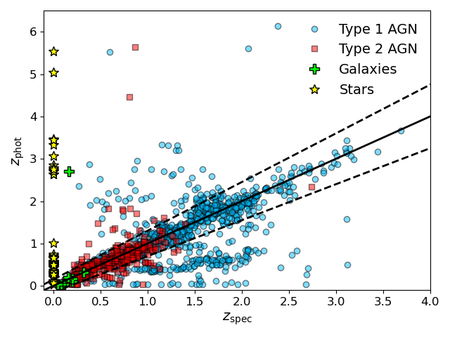
Figure 1: Stripe 82X photometric redshifts ($z_{\rm phot}$) compared with spectroscopic redshifts ($z_{\rm spec}$) for sources with spectroscopic redshifts obtained after the publication of the Stripe 82X DR2 photometric redshift catalog (Ananna et al., 2017). Subclasses of sources, identified by spectroscopic classification, are plotted separately as indicated by the legend. The solid line is the one-to-one relation while the dashed lines delineate the $|(z_{\rm spec}-z_{\rm phot})|/(1+z_{\rm spec})>0.15$ boundaries used to define significant outliers. Overall, the accuracy of the photometric redshifts (defined by the normalized median absolute deviation) is 0.08 with an outlier fraction of 24%.

Table 1: Stripe 82X Demographics

Category	Full Survey	XMM-AO10 & XMM-AO13
		($r<22$, AB)
X-ray Sources	6181	2194
Spectroscopic Redshifts	3457	1969
Spectroscopic Completeness	56%	90%
X-ray AGN	3211	1836
Type 1 AGN	2569	1490
Type 2 AGN	628	342
Optical, X-ray weak AGN	6	5
Galaxies	94	50
Stars	142	76
Area	31.3 deg2	20.2 deg2

3 Obscured AGN Demographics from Stripe 82X XMM-AO10 and XMM-AO13 at $r<22$

3.1 Defining Obscured AGN

Due to the homogeneous X-ray coverage and high level of spectroscopic completeness at $r<22$ (AB) in the XMM-AO10 and XMM-A013 portions of Stripe 82X, we explore the obscured AGN demographics within this subset of the survey. We focus on the 1836 X-ray AGN as the parent sample and consider three flavors of obscured AGN:

1. Optically obscured/Type 2 AGN (i.e., those that do no have broad lines in their spectra);

2. Reddened AGN ($R-K>4$, Vega), including both Type 1 and Type 2 AGN, though we caution that red $R-K$ colors for low-redshift AGN could be due to starlight rather than dust extinction (see, e.g., Glikman et al., 2022) and distinguishing between these scenarios is beyond the scope of this paper;

3. X-ray obscured AGN ($N_{\rm H}>10^{22}$ cm^-2).

We note that 6 X-ray AGN have spectroscopic redshifts but not classifications in the archival catalogs we queried, so we are we are therefore unable to classify them as optically unobscured or optically obscured. We thus can classify 1830 AGN as Type 1 or Type 2 based on the presence or absence of broad lines in their optical spectra in Table 2.

We follow the prescription in LaMassa et al. (2016b) and LaMassa et al. (2017) to convert the SDSS $r^{\prime}$ (AB) magnitude to the Bessell $R$ magnitude (Vega), using an $r-i$ color correction, to allow a more direct comparison with $R-K$-selected reddened AGN from the literature (e.g., Glikman et al., 2007, 2013; Brusa et al., 2010). As discussed in LaMassa et al. (2016b), the SDSS magnitudes are measured assuming a PSF model for point sources, or with an exponential profile or de Vaucoulers profile for extended sources, while the near-infrared magnitudes are measured through a larger 2.8^′′ or 5.6^′′ aperture for point and extended sources, respectively. Different portions of the host galaxy can thus be contributing to the optical and infrared magnitude measurements. However, as illustrated in LaMassa et al. (2016b), there are not signficant differences between the SDSS model magnitudes and a larger aperture “auto” magnitude measured via Source Extractor (Bertin & Arnouts, 1996) and published in the SDSS coadded catalog of (Jiang et al., 2014). The convention followed here is also consistent with precedent in the literature (e.g., Urrutia et al., 2009; Glikman et al., 2013).

There are two near-infrared surveys that cover Stripe 82: the VISTA Hemisphere Survey (VHS; McMahon et al., 2013) and the UKIRT Infrared Deep Sky Survey (UKIDSS; Lawrence et al., 2007). The VHS survey is slightly deeper than UKIDSS, with a 5$\sigma$ depth of $K=20.3$ (AB) compared with a 5$\sigma$ depth of $K=20.1$, respectively, and the VHS photometry has smaller errors than UKIDSS (see Figure 7 in Ananna et al., 2017). Similar to Ananna et al. (2017), we choose the VHS $K$-band photometry if available, but otherwise use the UKIDSS photometry. Since the magnitudes in the Stripe 82X catalog are reported in the AB system, we convert the $K$-band magnitude to Vega using $K_{\rm Vega}=K_{\rm AB}-1.9$. There are 1645 X-ray AGN that have available optical and infrared photometry to identify reddened AGN.

We use the X-ray spectral fitting catalog from Peca et al. (2023) for the $N_{\rm H}$ measurements to identify which AGN are X-ray obscured. For the spectral fitting to be performed, at least 20 net counts were required, though the minimum number of counts needed for a spectral fit varies as a function of AGN redshift and X-ray spectal model complexity (see Peca et al., 2023, for details). 1168 AGN have column density measurements from X-ray spectral fitting and can thus be classified as X-ray obscured ($N_{\rm H}>10^{22}$ cm^-2) or unboscured.

In Table 2, we list the number of AGN from the “parent” sample for each subclass, i.e., the number of sources where we have information to classify an AGN as “obscured” according to the metric considered, and the number of obscured AGN in each category. We find that 417 AGN (23%) are considered obscured by at least one of these metrics. The largest category of obscured AGN are Type 2 AGN, making up 19% of the population.

We note that the X-ray obscured AGN fraction reported here (10%) is likely a lower limit since heavily obscured AGN will have X-ray spectra of low quality or too few counts to permit spectral modeling to measure an obscuring column density. Indeed, after correcting for Stripe 82X survey biases, Peca et al. (2023) find an intrinsic X-ray obscured AGN fraction of $\sim$57% for X-ray luminosities above 10⁴³ erg s^-1. Our analysis is complementary to that of Peca et al. (2023) as they consider only X-ray obscured AGN while we include Type 2 and reddened AGN in this analysis. Additionally, we focus on just the XMM-AO10 and XMM-AO13 portions of the Stripe 82X survey at $r<22$ (AB) while Peca et al. (2023) consider the full Stripe 82X survey.

3.2 (Dis)Agreement Among Obscured AGN Classifications

In Figure 2 (left), we show a Venn diagram of these obscured AGN classifications, highlighting the population that is unqiue to one metric and where there is agreement among the definitions. We find that more than half of the X-ray obscured AGN are optically unobscured suggesting a distinction between the gas that attenuates X-ray photons and the more distant dust that obscures the broad line region, perhaps related to the radiation environment around the black hole (e.g., Merloni et al., 2014). Evidence of such high column density clouds within the broad line region dust sublimation zone have been observed in so called X-ray “changing-look” AGN (e.g., McKernan & Yaqoob, 1998; Risaliti et al., 2009; Marinucci et al., 2016)

When we limit this comparison to just the AGN that have both spectroscopic classifications and $N_{\rm H}$ measurements from X-ray spectral fitting (Figure 2, right), we see that only 18% of AGN are both obscured optically and in X-rays. This is a much lower fraction than reported in previous X-ray surveys. Samples of hard X-ray selected AGN (E $>$ 10 keV) in the local Universe from INTEGRAL (predominantly $z<0.1$; Bird et al., 2010) and Swift-BAT (mostly $z<0.4$; Baumgartner et al., 2013; Oh et al., 2018) find a 12% disrepancy and $\sim$2% discrepancy, respectively between optically and X-ray obscured AGN (Malizia et al., 2012; Koss et al., 2017). From the moderate-area, moderate-depth XMM-COSMOS survey (Hasinger et al., 2007; Cappelluti et al., 2009), spanning a similar redshift range as Stripe 82X ($0.3<z<3.5$) though sampling the moderate-luminosity AGN population, Merloni et al. (2014) find a 30% disagreement between optical and X-ray obscured AGN classifications. The most direct comparison to Stripe 82X is from the XMM-XXL-N field which covers a comparable area ($\sim$25 deg²) at a comparable depth (Pierre et al., 2016; Menzel et al., 2016). Compared with the other X-ray surveys, there is a larger discrepancy between X-ray and optically obscured AGN (Liu et al., 2016), but this fraction of 40% is still well below the $\sim$80% fraction we find in Stripe 82X. We note that the dividing column density between X-ray obscured and unobscured varies from $N_{\rm H}=10^{21.5}$ cm^-2 (Merloni et al., 2014; Liu et al., 2016) to $N_{\rm H}=10^{21.9}$ cm^-2 (Koss et al., 2017). However, when we experiment with a threshold of $N_{\rm H}\geq 10^{21}$ cm^-2 to classify an AGN as obscured, the fraction of overlapping Type 2 and X-ray obscured AGN only increases to $\sim$23% meaning that the larger disagreement in the overlap of obscured AGN between Stripe 82X and other surveys is not driven by the obscured AGN column density threshold. We also considered AGN whose upper limit on the fitted column density exceeds 10²² cm^-2: while this more expansive definition of X-ray obscured AGN increased the overall number to 596, the overlap between Type 2 and X-ray obscured AGN was only 19%.

Table 2: Stripe 82 XMM-AO10 & XMM-AO13 Obscured AGN Summary ($r<22$, AB)

Category	Parent sample	Number of Obscured AGN	Obscured AGN Fraction
Optically Obscured	1830	342	19%
(Type 2 AGN)
Reddened AGN	1645	39	2.4%
($R-K>4$)
X-ray Obscured	1168	111	10%
($N_{\rm H}>10^{22}$ cm-2)

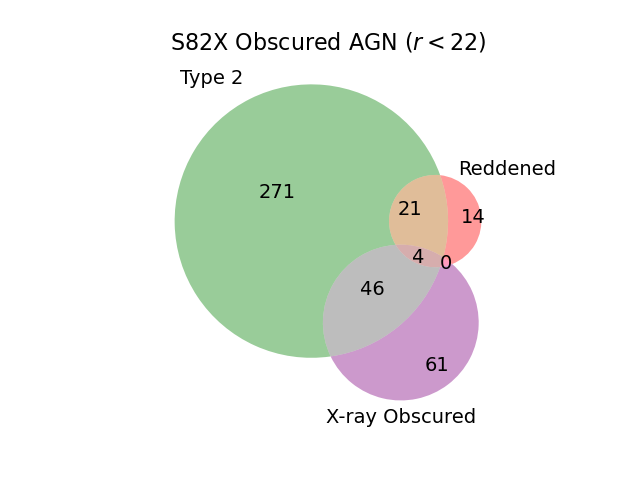
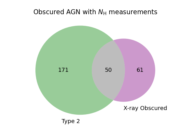
Figure 2: (Left:) Venn diagram showing classes of obscured AGN for all Stripe 82X AGN at $r<22$ with spectroscopic redshifts for the XMM-AO10 and XMM-AO13 portions of the survey. We distinguish among the following categories of obscured AGN: Type 2 AGN (i.e., no broad lines in optical spectra), reddened ($R-K>4$, Vega), and X-ray obscured ($N_{\rm H}>10^{22}$ cm^-2). (Right): Subset of obscured AGN that have both spectroscopic classifications and measured $N_{\rm H}$ values from X-ray spectral fitting; 121 of the Type 2 AGN shown in the left diagram do not have $N_{\rm H}$ measurements and are thus omitted from this figure. Of the 282 obscured AGN in this subset, only 18% are both Type 2 and X-ray obscured.

3.3 Luminosity - Redshift Distribution of Obscured AGN

We explore the luminosity-redshift parameter space inhabited by the spectroscopically identified Stripe 82X AGN at $r<22$ from XMM-AO10 and XMM-AO13 in Figure 3. We use the $k$-corrected, observed 2-10 keV luminosity ($L_{\rm X,observed}$) as a proxy of the AGN luminosity. We note that the intrinsic X-ray luminosity can be higher, but we only have $N_{\rm H}$ measurements and thereby intrinsic X-ray luminosities for a subset of the sample so we focus on the observed luminosity to not limit this analysis.

By design, Stripe 82X samples the high-luminosity AGN population. The top left panel of Figure 3 shows that, consistent with previous surveys and intrinsic X-ray luminosity functions that probe AGN beyond the local Universe (e.g., Merloni et al., 2014; Ueda et al., 2014; Buchner et al., 2015; Liu et al., 2017), the obscured AGN fraction dominates the population at lower luminosities and then decreases as luminosity increases (see Table 3 for a summary). These results are consistent with the “receding torus” model where increased radiation from higher luminosity AGN reduces the torus covering factor (Lawrence, 1991; Hönig & Beckert, 2007).

However, about a quarter of obscured AGN emit at the highest X-ray luminosities ($L_{\rm X}>10^{44}$ erg s^-1). Furthermore, as X-ray selection is biased against the Compton-thick population, heavily obscured AGN at higher luminosities can be altogether missing from Stripe 82X, neccesitating AGN samples selected at other wavelengths for a more comprehensive determination of the evolution of the intrinsic obscured AGN fraction with luminosity (e.g., Lusso et al., 2013; Mateos et al., 2017).

In the right hand panel of Figure 3, we consider the obscured AGN subpopulations separately. We find that the Type 2 AGN are predominantly at $z<1$ and luminosities below $L_{\rm X}<10^{44}$ erg s^-1, though there is a tail of the distribution at higher luminosities and up to redshifts of $z\sim 1.5$. The reddened AGN lie at redshifts $0.25<z<1.25$ and are at moderate to high X-ray luminosities ($L_{\rm X}\geq 10^{43.5}$ erg s^-1), though the number of Type 2 AGN at these luminosities is comparable to the number of reddened AGN. The most luminous ($L_{\rm X,observed}>10^{44.5}$ erg s^-1) obscured AGN are predominantly X-ray obscured: these AGN are Type 1 and are mostly not reddened, but based on X-ray spectral modeling, are attenuated by column densities $N_{\rm H}>10^{22}$ cm^-2.

In the bottom panel of Figure 3, we explore the luminosity-redshift space of AGN that are classified as obscured according to multiple metrics. The Type 2 + X-ray obscured AGN span the largest range in redshift ($0<z<1.25$) and luminosity ($10^{42}$ erg s${}^{-1}<L_{\rm X,observed}<10^{44.5}$ erg s^-1) while the reddened AGN + Type 2 and reddened AGN + Type 2 + X-ray obscured are at higher redshift ($z>0.25$) and luminosity ($L_{\rm X,observed}>10^{43}$ erg s^-1). Still, we see that the AGN that are only X-ray obscured (top right panel of Figure 3) extend to higher redshifts ($z>1.25$) and luminosities ($L_{\rm X,observed}>10^{44.5}$ erg s^-1) than those that are also reddened.

These results are consistent with the trends reported in Merloni et al. (2014) and summarized in Hickox & Alexander (2018) that Type 2 AGN tend to be at lower X-ray luminosities while the fraction of X-ray obscured and optically unobscured AGN increases with luminosity. These results are also consistent with those reported by Glikman et al. (2018) who found that, using a sample of mid-infrared color selected AGN, the fraction of reddened Type 1 AGN increases with luminosity while the opposite trend is seen for Type 2 AGN.

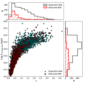
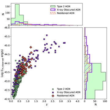
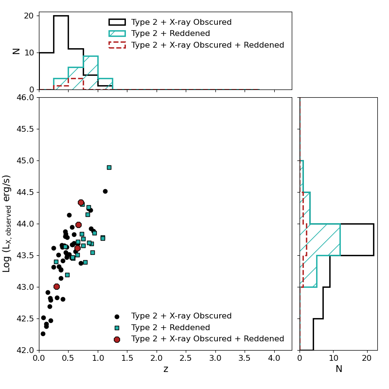
Figure 3: Observed, rest-frame 2-10 keV X-ray luminosity as a function of redshift for all spectroscopically identified AGN from Stripe 82 XMM-AO10 and XMM-AO13 at $r<22$. At these X-ray and optical flux limits, the Stripe 82X survey is 90% spectroscopically complete. (Left): Since Stripe 82X is a shallow, wide-area survey, it largely samples the high-luminosity AGN parameter space. The obscured AGN (Type 2 AGN, reddened AGN, and X-ray obscured AGN; red stars) are predominantly at lower luminosities and redshifts and make up the majority of low-luminosity ($L_{\rm X}<10^{43}$ erg s^-1) Stripe 82X AGN (see also Table 3). (Right): Of the obscured AGN population, the Type 2 AGN (green circles) are at the lowest luminosities and redshifts. The X-ray obscured AGN (where $N_{\rm H}>10^{22}$ cm^-2; purple squares) extend to high luminosities ($L_{\rm X}>10^{44.5}$ erg s^-1) and high redshifts ($z>1$). The reddened AGN (red crosses) are found at moderate-to-high X-ray luminosities, overlapping the tail of the Type 2 AGN $L-z$ distribution. There is some overlap in these sub-populations of obscured AGN (see Figure 2) (Bottom): Luminosity-redshift distribution for AGN that are classified as obscured based on multiple metrics (as indicated in the legend). The Type 2 + X-ray obscured AGN span a range of redshifts and luminosities, while the AGN that are reddened and also Type 2 and/or X-ray obscured are at higher luminosities ($L_{\rm X}=10^{43}$ erg s^-1 and mostly above $z>0.5$), but they do not extend to as high redshift or luminosity as the AGN that are only X-ray obscured.

Table 3: Observed Obscured AGN Fraction

$L_{\rm X,observed}$ Bin	Obscured AGN #	Obscured Fraction
Log (erg s-1)
42.0 - 42.5	51	84%
42.5 - 43.0	91	66%
43.0 - 43.5	110	47%
43.5 - 44.0	100	25%
44.0 - 44.5	37	6.9%
44.5 - 45.0	18	4.6%
$>$45.0	10	14%

4 Measuring Black Hole Masses for Type 1 AGN

We measure the black hole masses ($M_{\rm BH}$) of Type 1 AGN in Stripe 82X from SDSS single epoch spectroscopy using virial relations that were calibrated on results from reverberation mapping campaigns (see Peterson, 2014, for a review). These relations rely on measuring the continuum luminosity and width of broad emission lines in Type 1 AGN and take the form of:

$$\rm{Log}\left(\frac{M_{\rm BH,vir}}{M_{\rm\sun}}\right)=a+b\times\rm{Log}\left(\frac{L}{10^{44}\,\rm{erg}\rm{s}\,^{-1}}\right)+$$

$$c\times\rm{Log}\left(\frac{\rm{FWHM}}{{\rm km}\,{\rm s}^{-1}}\right),$$ (3)

where $L$ refers to the wavelength at which the AGN continuum luminosity is driving the line emission, FWHM is the measured full width half maximum of the broad emission line, and $a$, $b$, and $c$ are fitted constants from extrapolating reverberation mapping results to scaling relationships. Table 4 summarizes the scaling relations we used in this work. The uncertainties in black hole mass measurements is on the order of 0.4 dex for these relations (Shen & Liu, 2012). More information about each of the single epoch relations is given in Section 4.1 to motivate the preference we gave in selecting the reference $M_{\rm BH}$ value in the catalog.

Table 4: Single epoch $M_{\rm BH}$ formula parameters^a

Line	$L^{b}$	a	b	c	Reference
H$\beta$	$L_{\rm 5100\text{\AA}}$	0.91	0.50	2.0	Vestergaard & Peterson (2006)
H$\alpha$	$L_{\rm 5100\text{\AA}}$	0.807	0.519	2.06	Greene et al. (2010)
Mg II	$L_{\rm 3000\text{\AA}}$	0.74	0.62	2.0	Shen et al. (2011)
C IV	$L_{\rm 1350\text{\AA}}$	0.66	0.53	2.0	Vestergaard & Peterson (2006)
aParameters used in Equation 4 to calculate black hole masses.
bThe wavelength at which the AGN continuum luminosity that powers
the line emission is calculated.

4.1 Virial Mass Scaling Relations for Single Epoch Spectroscopy

Reverberation mapping campaigns have historically been restricted to nearby ($z<0.3$) AGN to allow for high signal-to-noise spectra (S/N $\sim$ 100) to be observed over the span of months to years to measure variability. As a result, most AGN with black hole masses measured from reverberation mapping campaigns are based on the response of the H$\beta$ line to the variability in the continuum (e.g., Peterson et al., 2002; Denney et al., 2010; Grier et al., 2012, 2017; Bentz & Katz, 2015). As H$\beta$ is the most common line used for reverberation mapped black hole masses, this single epoch spectroscopy scaling relation from Vestergaard & Peterson (2006) is the most reliable of the four we consider in this analysis.

The next most reliable single epoch spectroscopy scaling relation is that based on the ultraviolet Mg II line (Shen et al., 2011). At modest redshifts ($z>$0.9), H$\beta$ is no longer accessible in observed-frame optical spectra, making ultraviolet emission lines a useful diagnostic for measuring black hole masses at this redshift regime from spectra in large ground based optical surveys like SDSS. McLure & Jarvis (2002) pointed out that Mg II is a fair substitute for the H$\beta$ line as a virial black hole mass estimator due to their similar ionization potentials, indicating that the gas responsible for these emission lines lie at the same radius in the broad line region.

The H$\alpha$ scaling relation from Greene et al. (2010) is based on the radius-luminosity calibration in Bentz et al. (2009) which was defined using the H$\beta$ line. To derive black hole mass from H$\alpha$, Greene et al. (2010) converted the FWHM of H$\beta$ to H$\alpha$ using the formulism in Greene & Ho (2005). Most of the Type 1 AGN in Stripe 82X are at too high a redshift for H$\alpha$ to be observed, and we defer to the H$\beta$ scaling relation when possible since this calibration is based directly on reverberation mapped black hole measurements.

Finally, the ultraviolet C IV line can be used as a black hole estimator for higher redshift AGN ($z>$1.5) observed by SDSS. The C IV line mass estimator is controversial since asymmetries and blueshifts in the line profile (Marziani et al., 1996) and disagreements between C IV-based masses and those calculated from H$\beta$, H$\alpha$ and MgII (Netzer et al., 2007; Shen et al., 2008; Shen & Liu, 2012; Trakhtenbrot & Netzer, 2012) indicate that the gas producing C IV has significant contributions from non-virialized motion (Baskin & Laor, 2005; Shen et al., 2008), likely due to outflows for AGN exceeding $\sim$10% Eddington (Temple et al., 2023). However, monitoring campaigns of high redshift AGN show that the C IV line does reverberate in response to the AGN continuum variability (Kaspi et al., 2007; De Rosa et al., 2015; Grier et al., 2019), allowing C IV-based black hole masses to be calculated via reverberation mapping campaigns. We use the C IV viral mass estimator derived in Vestergaard & Peterson (2006), and note that a comparison between C IV reverberation mapped black hole masses and those from single epoch spectroscopy show that the latter values are systematically larger than the former (Lira et al., 2018), perhaps due to contributions from non-virial motion to the C IV line profile (Denney, 2012; Lira et al., 2018).

4.2 Spectral Decomposition of Stripe 82X Type 1 AGN

To derive the spectroscopic parameters needed to calculate $M_{\rm BH}$, we fitted the SDSS spectra of the 2235 Stripe 82X Type 1 AGN with PyQSOFit (Guo et al., 2018). This fitting package is the python version of the IDL codes used to calculate black hole masses in previous large SDSS quasar catalogs (e.g., Shen et al., 2011), so it is well trained on SDSS spectra and produces results that are directly comparable to published catalogs.

To perform the spectral decomposition, PyQSOFit fits a continuum that consists of powerlaw emission from the accretion disk, optical Fe II templates (Boroson & Green, 1992) and ultraviolet Fe II templates (Vestergaard & Wilkes, 2001) that produce a pseudo-continuum, a Balmer Continuum from 1000Å-3646Å (Dietrich et al., 2002), and a host galaxy that is fit by doing a principle component analysis (PCA) using eigenspectra derived from SDSS galaxy spectra (Yip et al., 2004). We modify this routine to replace the PCA method and to instead fit galaxy spectral templates from the E-MILES library (Vazdekis et al., 2016). However, in most cases the continuum was dominated by the AGN and the host galaxy was not detected, meaning that the host galaxy decomposition was not applied. The continuum is subtracted in windows around each emission line of interest, with the lines then fitted by broad and narrow components. PyQSOFit reports the fitted parameters on the continuum components, emission lines, and continuum luminosities ($L_{\rm 5100\text{\AA}}$, $L_{\rm 3000\text{\AA}}$, and $L_{\rm 1350\text{\AA}}$), with errors on fit parameters calculated via Monte Carlo resampling.

After fitting the SDSS spectra of Stripe 82X Type 1 AGN, we vetted the results. We rejected an emission line or continuum measurement if the:

• Fit parameter or error is non-finite (e.g., NaN);

• Error on a fit parameter (FWHM, $\sigma$, equivalent width, central wavelength of emission line, line flux) is greater than the fitted value of that parameter;

• FWHM is 0;

• Continuum luminosity is 0;

• FWHM $>$ 15,000 km/s which indicates that the Gaussian model is fitting residuals in the continuum and not the emission line.

For the line and continuum measurements that passed these checks, we then calculated black hole masses using Eq. 4 and the parameters in Table 4. We rejected any $M_{\rm BH}$ measurements where the error on the black hole mass exceeded the measured mass of the black hole.

We then visually inspected the fits to the remaining sources and discarded any $M_{\rm BH}$ value where the relevant emission line fit was poor. In these cases, the measured “line” was actually noise in the continuum or the continuum near the line was poorly measured which would bias both the continuum luminosity and the ability to accurately measure the emission line FWHM. We stress that within a spectrum, a fit can be discarded for one emission line but acceptable for another emission line.

4.3 Black Hole Masses of Stripe 82X Type 1 AGN

Of the 2235 SDSS spectra we fitted, we obtained an acceptable black hole measurement from at least 1 emission line for 1396 sources, representing 62% of the Type 1 Stripe 82X AGN with SDSS spectra. The number of AGN with black hole masses measured from each emission line single epoch formula are listed in Table 5. In our published catalog, we report the values for each of these measurements, as well as a reference M_BH value based on the ranking system described above (i.e., M_BH = 1. M_BH,Hβ; 2. M_BH,MgII; 3. M_BH,Hα; 4. M_BH,CIV). In Table 5, we list the number of sources for each line estimator that are reported as M_BH, as well as the redshift range and median redshift for the AGN in each subsample. We plot in Figure 4 the redshift distribution of all Stripe 82X Type 1 AGN, and those for which we calculated black hole masses, to illustrate that our measurements fully sample the spectroscopic redshift parameter space of Type 1 AGN in Stripe 82X.

Table 5: Black Hole Mass Tally

Line	Individual	MBH	$z$ range	Median $z$
	Measurements
H$\beta$	312	312	0.03 - 1.00	0.52
MgII	828	696	0.37 - 2.31	1.26
H$\alpha$	113	38	0.05 - 0.42	0.31
CIV	426	350	1.64 - 3.44	2.23

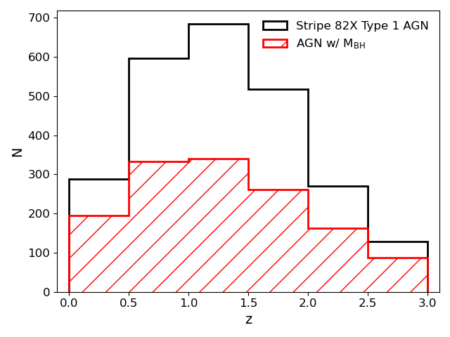
Figure 4: Redshift distribution of all Type 1 AGN in Stripe 82X with those that have black hole masses measured shown in the hatched region. The distributions are similar, indicating that our black hole mass subsample is not biased in redshift space relative to broad line AGN in Stripe 82X.

4.4 Comparison of Emission Line Single Epoch Mass Estimators

We compared the agreement of the black hole mass measurements for the AGN in which we have these results from more than one emission line. As shown in Figure 5, there are systematic differences when doing these pair-wise comparisons. We quantified these differences by calculating $\Delta$ = Log(M_BH,1) - Log(M_BH,2) and finding the average difference and dispersion in this residual, which we report in Table 6. In all cases, the dispersion ranges from a factor of 2 - 3, consistent with the systematic uncertainties in black hole mass measurements reported in the literature (e.g., Shen & Liu, 2012). We find the best agreement between the Balmer-derived black hole masses (average offset of $\sim$1.2), while the other values show average offsets of at least a factor of 2. We find that the black hole masses derived by the Balmer lines are a factor of two higher than those calculated from the Mg II line. Conversely, the Mg II-derived black hole mass is a factor of two higher than that calculated from the C IV line. Due to these systematic differences, we recommend that statistical analyses using these black hole mass measurements focus on black hole masses measured using the same emission line single epoch formula. We note that a comparable study was done on moderate luminosity ($10^{43}$ erg s${}^{1}<L_{\rm 2-10keV}<10^{45}$ eg s^-1) AGN from the COSMOS survey, and no systematic offsets between black hole masses from different emission lines was found: the black hole masses derived from the Balmer lines and the Mg II line were consistent within factors of 0.01 - 0.06 dex and dispersions of 0.27 - 0.42 dex (Schulze et al., 2018), though higher discrepancies were found when comparing black hole masses from the C IV line with those calculated from the H$\alpha$ and H$\beta$ lines (dispersions of 0.43 - 0.58 dex).

In the Appendix, we compare our black hole measurements with those published in Shen et al. (2011) for objects we have in common, demonstrating that we obtain roughly consistent results within an average factor of $<$1.1 for H$\beta$, $<$1.2 for Mg II, and $<$1.4 for C IV .

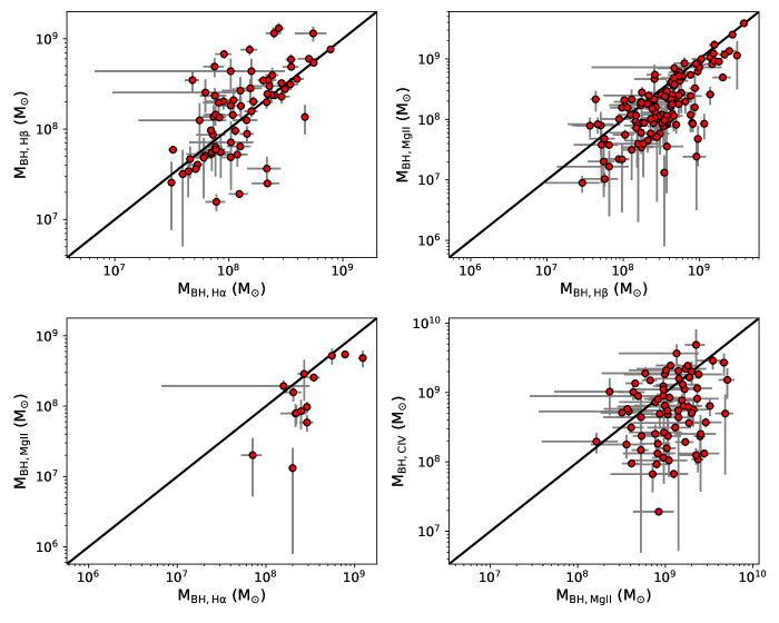
Figure 5: Intercomparison of black hole masses calculated from the various emission line single epoch formulas. We find systematic differences between these estimators. While this offset is lower for the Balmer lines (factor of $\sim$1.2), it it about a factor of 2 when comparing the Mg II-derived black hole mass with that calculating from the Balmer lines and between the Mg II and C IV derived black hole masses.

Table 6: Offsets in Black Hole Mass Measurements

$M_{\rm BH}$ Residual	Mean Residual	Dispersion
Log($M_{\rm BH,1}$) - Log($M_{\rm BH,2}$)	(dex)	(dex)
H$\beta$ - H$\alpha$	0.07	0.36
Mg II - H$\beta$	-0.30	0.36
Mg II - H$\alpha$	-0.35	0.32
C IV - Mg II	-0.33	0.51

In Figure 6 (left), we plot the distribution of the reference black hole masses (M_BH) for the Stripe 82X Type 1 AGN, and highlight the subsets of measurements that are derived via the various emission line single epoch formulas used in this analysis. Though we find that there are systematic differences when comparing black hole mass measurements for the same source using different emission line formulas (Figure 5 and Table 6), the opposite trends are apparent when we consider the full sample. That is, though the Balmer-derived black hole masses are a factor of two higher than the Mg II- derived black hole masses, the AGN with more massive black holes are those calculated from the Mg II and C IV emission lines. As we show in the right hand panel of Figure 6, the AGN with more massive black holes are more luminous (see Section 5 for $L_{\rm bol}$ calculation) and at higher redshift which is a more dominant effect than the systematic differences between Balmer- and Mg II-derived black hole mass measurement. Such a result is consistent with the previously reported trends of AGN cosmic downsizing where more massive black holes power higher luminosity AGN at earlier times in the Universe ($z\gtrsim 1$) than in the present day ($z\sim 0$; e.g., Barger et al., 2005; Ueda et al., 2014).

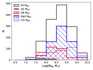
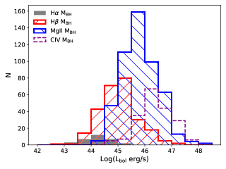
Figure 6: (Left): Distribution of black hole masses for Type 1 AGN where the individual emission line single epoch calculations that are chosen as the reference $M_{\rm BH}$ are plotted separately. Though the intercomparison of single epoch formulations show that the Balmer derived masses are on average a factor of two higher than the MgII masses, the higher mass black holes are found from the Mg II- and C IV-derived black hole mass measurements. (Right): Distribution of the AGN bolometric luminosity for the various black hole mass formulations, showing that the AGN with Mg II- and C IV-derived black hole masses are associated with more luminous AGN, which are also at higher redshift (see Table 5). This association explains why the Mg II- and C IV-derived black hole masses are larger than those calculated from the Balmer lines, despite the opposite systematic offsets observed in Figure 5.

5 Eddington Luminosity and Ratios

From the black hole mass, we calculate the Eddington Luminosity ($L_{\rm Edd}$), which is the luminosity at which radiation from the accretion disk balances gravity, with:

$$L_{\rm Edd}=1.26\times 10^{38}\ \frac{M_{\rm BH}}{{\rm M_{\rm\odot}}}.$$ (4)

The value of $L_{\rm Edd}$ in the published catalog is based on the reference black hole mass ($M_{\rm BH}$).

We can calculate the Eddington parameter, which serves as a proxy of the accretion rate, by dividing the bolometric AGN luminosity ($L_{\rm bol}$) by the Eddington luminosity:

$$\lambda_{\rm Edd}=L_{\rm bol}/L_{\rm Edd}$$ (5)

We use the intrinsic X-ray luminosity calculated via spectral fitting in Peca et al. (2023) to calculate $L_{\rm bol}$ using a bolometric luminosity dependent bolometric correction derived on a set of AGN that span almost 7 orders of magnitude in luminosity space (Duras et al., 2020).

From Duras et al. (2020), the bolometric luminosity for Type 1 AGN is given as:

$$\frac{L_{\rm bol}}{L_{\rm 2-10keV}}=12.76\left[1+\left(\frac{{\rm Log(L_{\rm bol}/L_{\rm\odot})}}{12.15}\right)^{18.87}\right].$$ (6)

Out of our sample of 1396 Stripe 82X Type 1 AGN with measured black hole masses, 998 have measured intrinsic X-ray luminosity values from Peca et al. (2023), and thus $L_{\rm bol}$ values. We solved the above equation numerically to calculate $L_{\rm bol}$ for each AGN and use these values in the right hand panel of Figure 6.

To explore Eddington ratio trends, we are cognizant of the systematic differences in Type 1 AGN black hole masses between the single epoch formulas. We thus calculate the Eddington ratios separately for all AGN whose reference black hole mass is from the H$\beta$ formula ($\lambda_{\rm Edd,H\beta}$; 265 sources) and those derived from the Mg II emission line ($\lambda_{\rm Edd,MgII}$; 506 sources). We choose both of these emission line single epoch measurements since as shown in Figure 6, these proxies span the full range of AGN luminosity and black hole mass values in this sample.

As shown in Figure 7, there is a range of Eddington ratios, though most of the Stripe 82X Type 1 AGN are accreting at rates below 10-30% Eddington. We find that AGN with the highest Eddington ratios are those with black hole masses derived from the MgII line. As we showed in Figure 6, these AGN are at higher luminosities, but they also have larger black hole masses: these effects do not cancel out in the Eddington ratio. The right hand panel of Figure 7 demonstrates that these more rapidly accreting black holes ($\lambda_{\rm Edd}>$ 0.3) are in more luminous AGN, consistent with the framework that a bulk of mass accretion occurs in a phase when the AGN is luminous (e.g., Kollmeier et al., 2006; Hopkins & Hernquist, 2009; Lusso et al., 2012). We see no strong trends of Eddington ratio with AGN redshift (Figure 7, bottom panel), though almost all super-Eddington AGN ($\lambda_{\rm Edd}>1$) are at higher redshift ($z>1$).

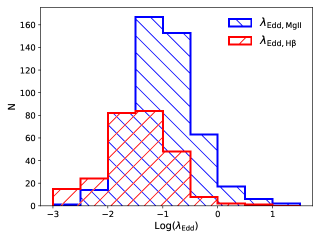
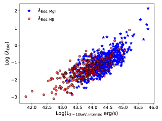
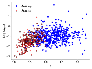
Figure 7: (Left): Distribution of the Eddington ratio ($\lambda_{\rm Edd}$) for Stripe 82X AGN that have intrinsic X-ray luminosities calculated via spectral fitting (Peca et al., 2023). Due to systematic differences in black hole mass measurements from the broad emission line single epoch formulas, we consider separately Type 1 AGN with reference black hole mass measurements derived from the Mg II line ($\lambda_{\rm Edd,MgII}$) and those derived from the H$\beta$ line ($\lambda_{\rm Edd,H\beta}$). The more rapidly accreting black holes ($\lambda_{\rm Edd}>0.3$) are those with Mg II-derived black hole masses. (Right): Eddington ratio plotted as a function of the intrinsic X-ray luminosity (L_{2-10keV,intrinsic}) demonstrating that luminous AGN ($>10^{45}$ erg s^-1) are associated with higher accretion rates. (Bottom): Eddington ratio as a function of redshift, showing no strong trends with cosmic time.

6 Conclusions

In this third data release of the 31.3 deg² Stripe 82X survey, we provide one comprehensive catalog that combines the X-ray, multiwavelength, and spectroscopic information published in previous releases (LaMassa et al., 2013a, b, 2016a, 2019; Ananna et al., 2017) with 343 new spectroscopic redshifts. We also calculated black hole masses for 1396 Type 1 AGN.

Stripe 82X is 56% spectroscopically complete: 3457 out of 6181 X-ray sources have secure spectroscopic redshifts. 93% of the X-ray sources with redshifts are AGN, with $L_{\rm X}>10^{42}$ erg s^-1. When considering the 20.2 deg² portion of the survey with homogenous X-ray coverage from XMM-Newton AO10 and AO13 (PI: Urry) that is brighter than $r=22$, this completeness rises to 90%. Focusing on this nearly complete portion of Stripe 82X, we find an obscured AGN fraction of 23%, most of which are Type 2 AGN (i.e., they lack broad lines in their optical spectra). Unlike other surveys, we find only 18% overlap between optically obscured and X-ray obscured ($N_{\rm H}>10^{22}$ cm^-2) AGN.

Using single epoch spectroscopy virial mass formulas, we calculated black hole masses for 1396 Type 1 AGN. There are systematic differences in $M_{\rm BH}$ for the same AGN depending on the emission line formula used. We encourage future statistical studies using Stripe 82X $M_{\rm BH}$ values to use black hole masses derived with the same formula. We found that most Stripe 82X AGN are accreting at sub-Eddington levels, and, consistent with previous studies, found that the most actively accreting black holes ($\lambda_{\rm Edd}>1$) are hosted in the most luminous AGN ($L_{\rm 2-10keV,intrinsic}>10^{45}$ erg s^-1) at $z>1$.

An upcoming Stripe 82X data release, Stripe 82-XL, will include additional archival X-ray observations and multi-wavelength counterparts, expanding the survey area to 57 deg² and totaling $\sim$23000 objects (Peca et al., on prep.). We are currently in the process of releasing a morphological catalog for AGN host galaxies in Stripe 82X using the Galaxy Morphology Posterior Estimation Network (GaMPEN; Ghosh et al., 2022) and PSFGAN (Tian et al., 2023).

Stripe 82X, the forthcoming $\sim$57 deg² Stripe 82-XL (Peca et al., in prep.) and other dedicted wide-area X-ray surveys like the 50 deg² XMM-XXL (Pierre et al., 2016; Liu et al., 2016; Menzel et al., 2016), 13.1 deg² XMM- Spitzer Extragalactic Representative Volume Survey (Chen et al., 2018; Ni et al., 2021, XMM-SERVS;), and 9.3 deg² Chandra Boötes survey (Masini et al., 2020), reveal the tip of the iceberg of luminous obscured black hole growth that can only be revealed by wide-area X-ray surveys. The eROSITA mission surveys the full sky in X-rays, with greatest sensivity in the soft 0.3-3.5 keV band (Predehl et al., 2021), and can leverage lessons learned from dedicated surveys like Stripe 82X to more fully probe high redshift obscured AGN at high luminosity, which is a population we are only beginning to understand. Already, the eROSITA Final Equatorial Depth Survey (eFEDS), completed during the eROSITA performance verification phase, covered $\sim$140 deg² and detected over 27,000 significant X-ray sources (Brunner et al., 2022), where 91% were associated with a secure multiwavelength counterpart (Salvato et al., 2022) and 80% were identied as AGN ($\sim$22,000 sources) based on their extragalactic spectroscopic or photometric redshifts (Liu et al., 2022). While the obscured AGN fraction is modest (8%, assuming a column density threshold of $N_{\rm H}=10^{21.5}$ cm^-2 to differentiate between obscured and unobscured), eFEDS and the subsequent eROSITA All-Sky Survey (eRASS1; Merloni et al., 2024), culminating in a 4-year survey catalog (Predehl et al., 2021), will provide valuable insight into obscured black hole growth at the highest luminosities.

Appendix A Stripe 82X Catalog Description

This Stripe 82X catalog release combines elements of Stripe 82X Data Release 1 (X-ray source properties, far-infrared and radio counterparts to X-ray sources; LaMassa et al., 2016a), Stripe 82X Data Release 2 (multiwavelength counterpart coordinates and photometry, and photometric redshifts; Ananna et al., 2017), spectroscopic redshifts from Stripe 82X SDSS-IV eBOSS (LaMassa et al., 2019), new spectroscopic redshifts and classifications, and the black hole masses calculated in this paper. We utilize data from the Chandra Source Catalog (Evans et al., 2010) for the archival Chandra sources in Stripe 82X (LaMassa et al., 2013a), where we required that a source be detected at $\geq$4.5$\sigma$ in at least one X-ray energy band (soft, hard, or full) for inclusion in the catalog. We performed source detection on all the XMM-Newton observations in Stripe 82X, both archival sources (LaMassa et al., 2013b) and the observations awarded to us in AO10 (LaMassa et al., 2013b) and AO13 (LaMassa et al., 2016a). We quantified the significance of an X-ray source detection using a minimum likelihood threshold: det_ml = -ln$P_{\rm random}$, where $P_{\rm random}$ is the Poissonian probability that an X-ray source detection is due to chance. To include an XMM source in the catalog, it had to be detected at a det_ml $\geq$ 15 (i.e., $>5\sigma$) level in at least one X-ray band.

When independently matching multiwavelength catalogs to the X-ray source list using a maximum likelihood estimator approach (Sutherland & Saunders, 1992), Ananna et al. (2017) defined a threshold likelihood ratio (LR) for each wavelength band above which they consider a match reliable. They also calculated a reliability value for each association following the procedure in Marchesi et al. (2016a). They found that different multiwavelength bands chose different counterparts for 12% of X-ray sources. In their analysis, they identified the most likely counterpart to each X-ray source and included the alternate counterparts as a reference, defining a quality flag (“QF”) to describe the conflicts. In this catalog, we chose the most likely counterpart and report the “QF” value for reference so users can assess the reliability of the association. All magnitudes are reported in the AB system. Ananna et al. (2017) used this multiwavelength catalog to generate spectral energy distributions (SEDs) that they fitted with LePhare (Arnouts & Ilbert, 2011) using a range of input SED templates to calculate photometric redshifts.

We describe the contents of the Stripe 82X catalog in Table 7. In Table 8, we list the number of Stripe 82X sources whose spectroscopic redshifts were collected from surveys and archival catalogs.

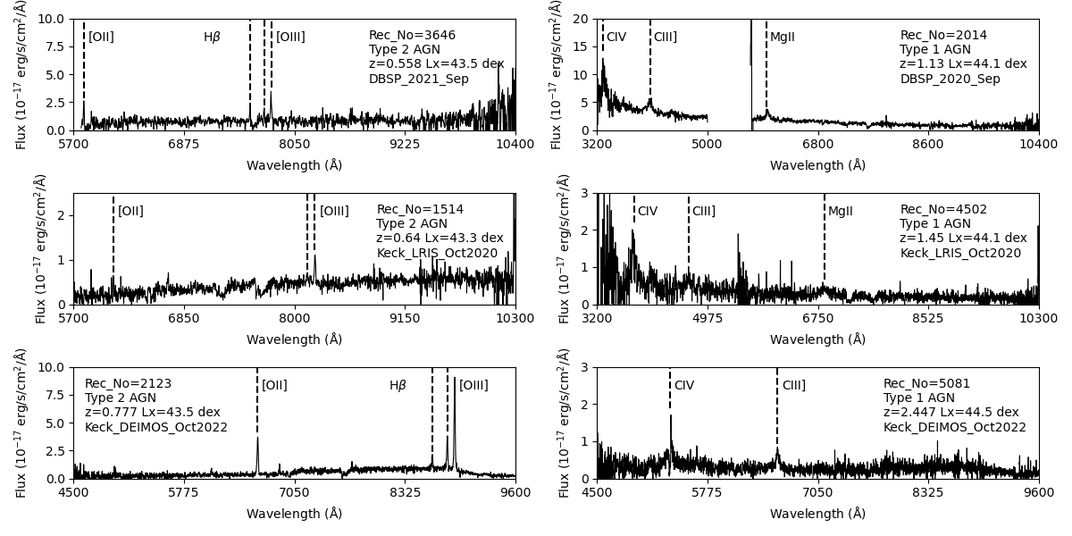
Figure 8: Example of spectra from our follow-up campaign with (top) Palomar DoubleSpec, (middle) Keck LRIS, and (bottom) Keck DEIMOS, illustrating both (left) Type 2 AGN and (right) Type 1 AGN. Identifying information is given in the legend of each plot, including estimated 2-10 keV luminosity and observing run in which spectrum was taken. Emission lines used to determine spectroscopic redshift are marked. Spectra from the red (blue) arm are Gaussian smoothed with a $\sigma$=1.0 ($\sigma$=1.5) kernel. The spectra are not telluric corrected nor do they have an absolute flux calibration applied.

In Table 9, we list the number of Stripe 82X sources with redshifts and classifications from our follow-up spectroscopic campaign. Details about the observing set-ups for our ground-based campaign are given in Table 10. Spectra obtained prior to 2018 were reduced with IRAF or SPEXTOOL (for Palomar TripleSpec spectra; Cushing et al., 2004; LaMassa et al., 2017) while infrared (optical) spectra obtained after 2018 (2020) were reduced with PypeIt (Prochaska et al., 2020a, b). The spectroscopic redshifts published here for the first time are those obtained after 2015 September, with the exception of the infrared spectra from Gemini GNIRS (2015) and Palomar TripleSpec (2015) which were published in LaMassa et al. (2017). A handful of optical spectra from our follow-up are shown in Figure 8 for illustrative purposes.

Table 7: Descripton of Stripe 82X Catalog Columns

Column Name	Description
MSID	Chandra Source Catalog (Evans et al., 2010) identifier; set to 0 for XMM sources.
REC_No	Stripe 82X identifier number for archival and AO10 and AO13 XMM sources; set to 0 for Chandra sources.
ObsID	XMM or Chandra Observation ID number for observation in which source is detected
Xray_Src	Provenance of X-ray source. Possible values are “Chandra”, “XMM_archive”, “XMM_AO10”, or “XMM_AO13”.
Xray_RA, Xray_Dec	Right Ascension and Declination of X-ray source.
Xray_RADec_Err	Astrometric error on the X-ray source coordinates.
Soft_Flux, Hard_Flux, Full_Flux	Observed flux (erg s-1 cm2) in the soft (0.5-2 keV), hard (2-10 keV for XMM; 2-7 keV for Chandra), and full (0.5-10 keV for XMM; 0.5-7 keV for Chandra) bands. A powerlaw model with $\Gamma=2.0$ ($\Gamma=1.7$) is assumed to convert count rates to flux for the soft (hard and full) bands. Users are advised to check det_ml for significance of flux measurement.
Soft_Flux_Error, Hard_Flux_Error, Full_Flux_Error	Error on the soft, hard, and full band fluxes (erg s-1 cm2). Values are for XMM sources only.
Soft_Flux_Error_High, Hard_Flux_Error_High, Full_Flux_Error_High	Higher bound on the soft, hard, and full band fluxes (erg s-1 cm2). If corresponding flux measurements are zero, these values represent the upper limit. Values are for Chandra sources only.
Soft_Flux_Error_Low, Hard_Flux_Error_Low, Full_Flux_Error_Low	Lower bound on the soft, hard, and full band fluxes (erg s-1 cm2). Values are for Chandra sources only.
Soft_Counts, Hard_Counts, Full_Counts	Net counts in the soft, hard, and full bands.
Soft_DetML, Hard_DetML, Full_DetML	Significance of detection in soft, hard, and full band, given by ${\it det\_ml}=-{\rm ln}P_{\rm random}$. For all significant Chandra detections, det_ml is set to a fiducial value of 11.0439, representing a 4.5$\sigma$ detection which we required to include a source in the LogN-LogS analysis in LaMassa et al. (2013a, 2016a). For the XMM sources, we required det_ml $\geq$15 to include a source in the LogN-LogS analysis of LaMassa et al. (2013b, 2016a).
Soft_Lum, Hard_Lum, Full_Lum	$k$-corrected luminosity in the soft, hard, and full bands, calculated for sources with a spectroscopic redshift and where det_ml $>$10 in that band. Units are in erg s-1. Luminosities are reported in log space.
CP_RA, CP_Dec	Coordinates of multiwavelength counterpart to X-ray source. Coordinates may be from SDSS, then VHS, then Spitzer. See Ananna et al. (2017) for details.
QF	Quality flag of multiwavelength counterpart (see Ananna et al. (2017) for details):
	0 No association found, or counterpart is from the LaMassa et al. (2016a) catalog.
	1 Unambiguous association.
	1.5 Conflicting associations, but a secure match in one band helps to resolve ambiguity.
	2 Counterparts disagree among multiwavelength bands matched to X-ray source, but the counterpart in one band exceeds the LR threshold to accept the association as the true counterpart, while the LR value was below the threshold in the other band.
	3 Counterparts disagree among multiwavelength bands and the LR values are comparable. The association with the greater reliability value is chosen as the counterpart.
	4 A counterpart is found in only one multiwavelength band.
mag_FUV, magerr_FUV, mag_NUV, magerr_NUV	GALEX far ultraviolet (FUV) and near ultraviolet (NUV) magnitudes and errors (AB; Morrissey et al., 2007). Extinction-corrected.
u, u_err, g, g_err, r, r_err, i, i_err, z, z_err	Optical SDSS magnitudes and errors (AB) from the coadded catalogs of Fliri & Trujillo (2016) (if available), otherwise from Jiang et al. (2014). Extintion-corrected when extinction information is available.
JVHS, JVHS_err, HVS, HVHS_err, HVHS_err, KVHS, KVHS_err	Near-infrared magnitudes and errors (AB) from the VISTA VHS survey in the $J$, $H$, and $K$ bands, using a 2.8′′ (5.6′′) radius aperture for point (extended) sources (McMahon et al., 2013). Extinction-corrected.
JUK, JUK_err, HUK, HUK_err, HUK_err, KUK, KUK_err	Near-infrared magnitudes and errors (AB) from the UKIDSS Large Area Survey survey in the $J$, $H$, and $K$ bands, using a 2.8′′ (5.6′′) radius aperture for point (extended) sources (Lawrence et al., 2007). Extinction-corrected.
CH1_SpIES, CH1_SpIES_err, CH2_SpIES, CH2_SpIES_err	Spitzer IRAC channel 1 (3.6 $\mu$m) and channel 2 (4.5 $\mu$m) magnitudes and error (AB) from the SpIES survey (Timlin et al., 2016). Not extinction-corrected.
CH1_SHELA, CH1_SHELA_err, CH2_SHELA, CH2_SHELA_err	Spitzer IRAC channel 1 (3.6 $\mu$m) and channel 2 (4.5 $\mu$m) magnitudes and error (AB) from the SHELA survey (Papovich et al., 2016). Not extinction-corrected.
W1, W1_err, W2, W2_err, W3, W3_err, W4, W4_err	AllWISE (Cutri et al., 2021) instrumental profile-fit photometry (w$n$mpro, where $n$ refers to band number) and error for point sources or elliptical aperture magnitude and error (w$n$gmag) for extended sources (where WISE_Ext is set to “YES”). W1, W2, W3, and W4 refer to magnitudes at 3.4$\mu$m, 4.6$\mu$m, 12$\mu$m, and 22$\mu$m, respectively. Reported magnitudes in this catalog are in AB system. Not extinction-corrected.
W1_SNR, W2_SNR, W3_SNR, W4_SNR	Signal-to-noise ratio for each WISE band. WISE magnitudes with S/N $<$ 2 should be considered an upper limit.
W1_Sat, W2_Sat, W3_Sat, W4_Sat	Fraction of pixels affected by saturation in each WISE band.
WISE_Ext	Flag to indicate if WISE source is extended. Reported magnitudes refer to elliptical magnitudes if set to “YES.”
FIRST_RA, FIRST_Dec	Coordinates of radio counterpart from FIRST survey (White et al., 1997).
FIRST_Dist	Distance (in arcseconds) between X-ray source and FIRST counterparts. Due to the low space density of FIRST sources, counterparts were found using nearest neighbor matching in LaMassa et al. (2016a).
FIRST_Flux, FIRST_Flux_Err	Integrated flux density and error at 1.4 GHz (mJy) from FIRST survey (White et al., 1997).
HERS_RA, HERS_Dec	Coordinates of far-infrared Herschel counterpart to X-ray source (Viero et al., 2014).
HERS_Dist	Distance (in arcseconds) between X-ray source and Herschel counterparts. Due to the low space density of Herschel sources, counterparts were found using nearest neighbor matching in LaMassa et al. (2016a).
F250, F250_Err, F350, F350_Err, F500, F500_Err	Flux density and $1\sigma$ error at 250$\mu$m, 350$\mu$m, and 500$\mu$m (mJy) from Herschel HeRS survey (Viero et al., 2014).
spec_z	Spectroscopic redshift.
spec_class	Spectroscopic classification.
z_src	Source of spectroscopic redshift and classification. See Table 8 for spectroscopic information from surveys and archival catalogs and Tables 9 - 10 for spectroscopic information from our ground-based follow-up campaign.
photo_z	Best-fit photometric redshift (see Ananna et al. (2017) for details).
PDZ_best	Confidence on photometric redshift.
Photo_z_sec	Secondary photometric redshift with a fit quality close to that of photo_z.
PDZ_sec	Confidence on secondary photometric redshift.
SED_morphology	Morphology of source according to SED template fitting for calculating photo_z with LePhare (Arnouts & Ilbert, 2011): 1. Star 2. Elliptical galaxy 3. Spiral galaxy 4. Type 2 AGN 5. Starburst galaxy 6. Type 1 AGN 7. QSO
Morphology	Source morphology according to optical or NIR photometry: point-like, extended, or uncertain (see Ananna et al., 2017).
M_BH, M_BH_err	Reference black hole mass and error in units of M⊙.
M_BH_Src	Emission line single epoch formula used to derive M_BH. We used the following ranked ordering as described in the main text: 1. H$\beta$ emission line formula from Vestergaard & Peterson (2006); 2. MgII emission line formula from Shen et al. (2011); 3. H$\alpha$ emission line formula from Greene et al. (2010); 4. CIV emission line formula from Vestergaard & Peterson (2006);
L_Edd, L_Edd_err	Eddington luminosity and error calculated from reference M_BH.
M_BH_HB, M_BH_HB_err, M_BH_MgII, M_BH_MgII_err, M_BH_Ha, M_BH_Ha_err, M_BH_CIV, M_BH_CIV_err	Black hole masses and errors derived from the H$\beta$ (Vestergaard & Peterson, 2006), MgII (Shen et al., 2011), H$\alpha$ (Greene et al., 2010), and CIV (Vestergaard & Peterson, 2006) formulas, respectively, in units of M⊙. Due to sysystematic offsets between the relations, we recommend that statistical analyses use black hole masses calculated using the same formula.
Xray_Lum	Estimate of the observed $k$-corrected hard band (2-10 keV) X-ray luminosity from the X-ray count rate. This value represents the hard band X-ray luminosity if there is a significant detection in the hard band. Otherwise, the X-ray luminosity in the full or soft band is scaled to derive $L_{\rm X}$, as described in the main text. This value is only calculated for sources with spectroscopic redshifts that are extragalactic. Luminosity is in units of erg s-1 and is reported in log space. For intrinsic X-ray luminosities derived via X-ray spctral fitting, see Peca et al. (2023).
Xray_AGN	If Xray_Lum exceeds 1042 erg s-1, this flag is set to “True.”

Table 8: Spectroscopic Redshifts from Surveys and Archival Catalogs

Catalog ID	Number	Reference
2SLAQ	67	2dF-SDSS QSO survey Croom et al. (2009)
6dF	6	6dF Galaxy Survey Jones et al. (2004, 2009)
DEEP2	9	Newman et al. (2013)
eBOSS_S82X	616	SDSS-IV eBOSS survey of Stripe 82X LaMassa et al. (2019)
Jiang2006	4	Spectroscopic survey of faint quasars in Stripe 82 (Jiang et al., 2006)
pre-BOSS	6	pre-SDSS BOSS survey (Ross et al., 2012)
PRIMUS	12	Coil et al. (2011)
SDSS_DR7Q	46	SDSS Quasar Catalog, Seventh Data Release (Schneider et al., 2010)
SDSS_DR8	4	Eighth Data Release of SDSS (Aihara et al., 2011)
SDSS_DR9	4	Ninth Data Release of SDSS (Ahn et al., 2012)
SDSS_DR12	43	Eleventh and Twelfth Data Releases of SDSS (Alam et al., 2015)
SDSS_DR12Q	511	SDSS Quasar Catalog, Twelfth Data Release (Pâris et al., 2017)
SDSS_DR13	975	Thirteenth Data Release of SDSS (Albareti et al., 2017)
SDSS_DR14	33	Fourteenth Data Release of SDSS (Abolfathi et al., 2018)
SDSS_DR14Q	490	SDSS Quasar Catalog, Fourteenth Data Release (Pâris et al., 2018)
SDSS_DR16	107	Sixteenth Data Release of SDSS (Ahumada et al., 2020)
sdss_correction	2	SDSS spectra where the reported redshift was incorrect and we report the correct redshift based on an independent calculation
SDSS_zwarning_verified_by_eye	13	SDSS spectra where the z_warning flag was set but we verified via visual inspection that the redshift and classification are acceptable
VVDS	24	Vimos VLT Deep Survey (Le Fèvre et al., 2004, 2005, 2013; Garilli et al., 2008)
WiggleZ	7	Drinkwater et al. (2010)

Table 9: Spectroscopic Redshifts from Dedicated Follow-up Campaigns

Catalog ID	Number	UT Observing Date
HYDRA_2012_Dec	14	2012 Dec 12 - Dec 13; 2012 Dec 17
HYDRA_2013_Aug_Sep	22	2013 Aug 31 - Sep 2
HYDRA_2014_Jan	44	2014 Jan 5 - Jan 7
HYDRA_2014_Jun	12	2014 Jun 21 - Jun 22
HYDRA_2014_Jul	29	2014 Jul 24 - Jul 28
DBSP_2014_Jul	4	2024 Jul 23 - Jul 24
Keck_NIRSPEC_2014	1	2014 Sep 7
DBSP_2014_Dec	1	2014 Dec 23
HYDRA_2015_Jan	1	2015 Jan 15 - Jan 16
DBSP_2015_Sep	22	2015 Sep 8 - Sep 11
DBSP_2015_Oct	7	2015 Oct 13 - Oct 17
Gemini_GNIRS_2015	3	2015 Dec 10; 2016 Jan 2; 2016 Jan 5; 2016 Jan 7; 2016 Jan 8
Palomar_TSpec_2015	4	2015 Oct 27
DBSP_2016_Aug	25	2016 Aug 28 - Aug 31
DBSP_2016_Sep	42	2017 Sep 24 - Sep 28
DBSP_2017_Jul	2	2017 Jul 27 - Jul 28
DBSP_2017_Aug	18	2017 Aug 27 - Aug 28
DBSP_2017_Sep	1	2017 Sep 1
Keck_LRIS_Sep2017	1	2017 Sep 16
Keck_LRIS_Oct2017	16	2017 Oct 17 - Oct 18
DBSP_2017_Oct	17	2017 Oct 27 - 28
Keck_NIRES_Sep2018	6	2018 Sep 17; 2018 Sep 19
Gemini_GNIRS_2019	1	2019 Sep 11; 2019 Oct 25
Keck_NIRES_Oct2019	8	2019 Oct 15
Palomar_TSpec_Oct2019	3	2019 Oct 16 - Oct 21
DBSP_2020_Sep	18	2020 Sep 23 - Sep 24
Keck_NIRES_Oct2020	5	2020 Oct 7
Keck_LRIS_Oct2020	17	2020 Oct 11
DBSP_2021_Jul	23	2021 Jul 7 - Jul 8; 2021 Jul 16 - Jul 18
DBSP_2021_Sep	30	2021 Sep 28 - Oct 1
KECK_DEIMOS_Oct2022	15	2022 Oct 3 - Oct 4
Keck_NIRES_Oct2022	1	2022 Oct 5
DBSP_2022_Oct	65	2022 Oct 4 - Oct 5; 2022 Oct 17 - Oct 20

Table 10: Instrument Set-up for Follow-up Observing Campaign

“z_src” prefix	Observatory	Instrument	Wavelength Coverage	Notes	References
Optical Instruments
HYDRA	WIYN	HYDRA	3000 - 8000 $\rm{\AA}$	Multi-object spectrograph	Barden & Armandroff (1995)
DBSP	Palomar	DoubleSpec	3200 - 5500 $\rm{\AA}$ (blue)	Single slit;	Oke & Gunn (1982)
			4700 - 10500 $\rm{\AA}$ (red)	separate blue and red arms	Rahmer et al. (2012)
KECK_LRIS	Keck	Low Resolution	3150 - 5400 $\rm{\AA}$ (blue)	Single slit;	Oke et al. (1995)
		Imaging Spectrometer	5650 - 10300 $\rm{\AA}$ (red)	separate blue & red arms	Rockosi et al. (2010)
KECK_DEIMOS	Keck	DEep Imaging Multi-	4500 - 6990 $\rm{\AA}$ (blue)	Used in single slit mode;	Faber et al. (2003)
		Object Spectrograph	7000 - 9630 $\rm{\AA}$ (red)	separate blue & red arms
Infrared Instruments
Keck_NIRSPEC	Keck	NIRSPEC	1.95 - 2.3 $\mu$m	Echelle	McLean et al. (1998)
Palomar_TSpec	Palomar	Triple Spectrograph	1.0 - 2.4 $\mu$m	Echelle	Herter et al. (2008)
Gemini_GNIRS	Gemini	Gemini Near-	0.8 - 2.5 $\mu$m	Echelle	Elias et al. (1998)
		Infrared Spectrograph
Keck_NIRES	Keck	Near-Infrared Echellete	0.94 - 2.45 $\mu$m	Echelle	Wilson et al. (2004)
		Spectrometer			Kassis et al. (2018)

Appendix B Comparing Stripe 82X Type 1 AGN with SDSS Type 1 AGN

Due to the systematic differences found in black hole masses for the same AGN when using different broad emission line single epoch formulas, we compare our measurements with those derived in Shen et al. (2011). Shen et al. (2011) fit the SDSS spectra of over a hundred thousand Type 1 quasars from the SDSS Data Release 7 (DR7; Abazajian et al., 2009) quasar catalog (Schneider et al., 2010). We cross matched the Type 1 AGN from Stripe 82X that have black hole measurements with those from the Shen et al. (2011) catalog that have black hole measurements using the same formulas we used. The results are shown in Figure 9, indicating that our measurements agree to within an average value of 10-40%, albeit with a spread of up to a factor of 2. The largest discrepancy is with the C IV black hole mass measurements which could be due to complexities with fitting a line profile that is often asymmetric. Still, we do not see systematic offsets observed in the Stripe 82X Type 1 AGN intercomparisons.

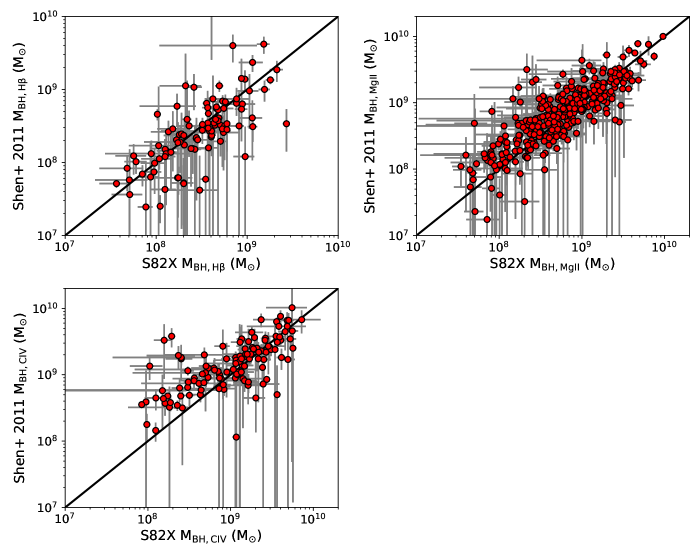
Figure 9: Comparison of black hole masses for Stripe 82X Type 1 AGN with those that have black hole mass measurements in Shen et al. (2011) using the same formulas. The values are roughly consistent, with residual values (i.e., Log($M_{\rm BH,S82X}$) - Log($M_{\rm BH,Shen2011}$)) of: $M_{\rm BH,H\beta}$ = 0.04 $\pm$ 0.36 dex, $M_{\rm BH,MgII}$ = -0.08 $\pm$ 0.28 dex, $M_{\rm BH,CIV}$ = -0.14 $\pm$ 0.35 dex.

Since we obtain on average consistent black hole measurements for the same AGN using the same formulas as the Shen et al. (2011) catalog, we propose that intrinsic reddening of the AGN host galaxy can be driving the Stripe 82X discrepancies. Photometrically blue sources were targeted as quasar candidates for spectroscopy in SDSS (Richards et al., 2002), while X-ray selection in Stripe 82X selects both blue and reddened AGN. As we show in Figure 10, the Type 1 AGN in Stripe 82X with SDSS spectra have on average redder colors than the Type 1 AGN in SDSS (Shen et al., 2011), with a median ($i-z$) color of 0.16 for Stripe 82X compared with 0.05 for SDSS Type 1 quasars. PyQSOFit corrects for Galactic reddening but does not model reddening in the host galaxy, meaning that the ultraviolet part of the spectrum, where the Mg II and C IV emission lines form, will be attenuated compared with the redder part of the spectrum containing the Balmer lines. We would then expect that the black hole masses derived from the ultraviolet lines would be systematically lower than those derived from the Balmer lines, which we observe in Figure 5.

However, when we inspect the intercomparison of black hole masses for Type 1 AGN in Stripe 82X in bins of ($i-z$) color (Figure 11), we see that optical reddening does not fully explain these offsets. We would expect the effects of reddening to be most pronounced when comparing black hole masses derived from the Mg II line and H$\beta$ line and from the C IV line and Mg II line. When comparing the Mg II-derived black hole masses with those calculated from the H$\beta$ line, we find that the redder sources ($0.25<$($i-z$)$<0.5$) are more offset (-0.40 dex) than the bluer sources ($0.0<$($i-z$)$<0.25$), but these blue sources still show an average offset of -0.21 dex. Furthermore, the AGN with both Mg II and C IV black hole masses are mostly blue (($i-z$) $<0.25$) though there is still a systematic offset with $M_{\rm BH,MgII}$ on average 0.33 dex larger than $M_{\rm BH,CIV}$.

Figure 10: Comparison of $(i-z)$ colors for Stripe 82X Type 1 AGN for which we calculated black hole masses from the SDSS spectra and all SDSS Type 1 quasars from the Shen et al. (2011) catalog, selected from the SDSS DR7 quasar catalog (Schneider et al., 2010). The Stripe 82X Type 1 AGN are on average redder (median ($i-z$) = 0.16) than the optically selected SDSS quasars (median ($i-z$) = 0.05). For both samples, we used SDSS magnitudes that were corrected for Galactic extinction to calculate the ($i-z$) color.

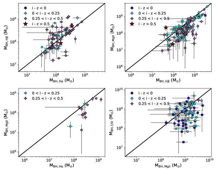
Figure 11: Comparison of Stripe 82X Type 1 AGN black hole masses in bins of ($i-z$) color. Systematic offsets between black hole masses can not be solely explained by optical reddening.

References

- Abazajian et al. (2009) Abazajian, K. N., Adelman-McCarthy, J. K., Agüeros, M. A., et al. 2009, ApJS, 182, 543. doi:10.1088/0067-0049/182/2/543
- Abolfathi et al. (2018) Abolfathi, B., Aguado, D. S., Aguilar, G., et al. 2018, ApJS, 235, 42. doi:10.3847/1538-4365/aa9e8a
- Ahn et al. (2012) Ahn, C. P., Alexandroff, R., Allende Prieto, C., et al. 2012, ApJS, 203, 21. doi:10.1088/0067-0049/203/2/21
- Ahumada et al. (2020) Ahumada, R., Allende Prieto, C., Almeida, A., et al. 2020, ApJS, 249, 3. doi:10.3847/1538-4365/ab929e
- Aihara et al. (2011) Aihara, H., Allende Prieto, C., An, D., et al. 2011, ApJS, 193, 29. doi:10.1088/0067-0049/193/2/29
- Aird et al. (2015) Aird, J., Coil, A. L., Georgakakis, A., et al. 2015, MNRAS, 451, 1892. doi:10.1093/mnras/stv1062
- Alam et al. (2015) Alam, S., Albareti, F. D., Allende Prieto, C., et al. 2015, ApJS, 219, 12. doi:10.1088/0067-0049/219/1/12
- Albareti et al. (2017) Albareti, F. D., Allende Prieto, C., Almeida, A., et al. 2017, ApJS, 233, 25. doi:10.3847/1538-4365/aa8992
- Antonucci (1993) Antonucci, R. 1993, ARA&A, 31, 473. doi:10.1146/annurev.aa.31.090193.002353
- Ananna et al. (2017) Ananna, T. T., Salvato, M., LaMassa, S., et al. 2017, ApJ, 850, 66. doi:10.3847/1538-4357/aa937d
- Ananna et al. (2019) Ananna, T. T., Treister, E., Urry, C. M., et al. 2019, ApJ, 871, 240. doi:10.3847/1538-4357/aafb77
- Annis et al. (2014) Annis, J., Soares-Santos, M., Strauss, M. A., et al. 2014, ApJ, 794, 120. doi:10.1088/0004-637X/794/2/120
- Arnouts & Ilbert (2011) Arnouts, S. & Ilbert, O. 2011, Astrophysics Source Code Library. ascl:1108.009
- Arrabal Haro et al. (2023) Arrabal Haro, P., Dickinson, M., Finkelstein, S. L., et al. 2023, ApJ, 951, L22. doi:10.3847/2041-8213/acdd54
- Astropy Collaboration et al. (2013) Astropy Collaboration, Robitaille, T. P., Tollerud, E. J., et al. 2013, A&A, 558, A33. doi:10.1051/0004-6361/201322068
- Astropy Collaboration et al. (2018) Astropy Collaboration, Price-Whelan, A. M., Sipőcz, B. M., et al. 2018, AJ, 156, 123. doi:10.3847/1538-3881/aabc4f
- Astropy Collaboration et al. (2022) Astropy Collaboration, Price-Whelan, A. M., Lim, P. L., et al. 2022, ApJ, 935, 167. doi:10.3847/1538-4357/ac7c74
- Barden & Armandroff (1995) Barden, S. C. & Armandroff, T. 1995, Proc. SPIE, 2476, 56. doi:10.1117/12.211839
- Baron & Ménard (2019) Baron, D. & Ménard, B. 2019, MNRAS, 487, 3404. doi:10.1093/mnras/stz1546
- Barger et al. (2005) Barger, A. J., Cowie, L. L., Mushotzky, R. F., et al. 2005, AJ, 129, 578. doi:10.1086/426915
- Baskin & Laor (2005) Baskin, A. & Laor, A. 2005, MNRAS, 356, 1029. doi:10.1111/j.1365-2966.2004.08525.x
- Baumgartner et al. (2013) Baumgartner, W. H., Tueller, J., Markwardt, C. B., et al. 2013, ApJS, 207, 19. doi:10.1088/0067-0049/207/2/19
- Becker et al. (1995) Becker, R. H., White, R. L., & Helfand, D. J. 1995, ApJ, 450, 559. doi:10.1086/176166
- Bentz et al. (2009) Bentz, M. C., Peterson, B. M., Netzer, H., et al. 2009, ApJ, 697, 160. doi:10.1088/0004-637X/697/1/160
- Bentz et al. (2013) Bentz, M. C., Denney, K. D., Grier, C. J., et al. 2013, ApJ, 767, 149. doi:10.1088/0004-637X/767/2/149
- Bentz & Katz (2015) Bentz, M. C. & Katz, S. 2015, PASP, 127, 67. doi:10.1086/679601
- Bertin & Arnouts (1996) Bertin, E. & Arnouts, S. 1996, A&AS, 117, 393. doi:10.1051/aas:1996164
- Bird et al. (2010) Bird, A. J., Bazzano, A., Bassani, L., et al. 2010, ApJS, 186, 1. doi:10.1088/0067-0049/186/1/1
- Blanton et al. (2017) Blanton, M. R., Bershady, M. A., Abolfathi, B., et al. 2017, AJ, 154, 28. doi:10.3847/1538-3881/aa7567
- Bogdan et al. (2023) Bogdan, A., Goulding, A., Natarajan, P., et al. 2023, arXiv:2305.15458. doi:10.48550/arXiv.2305.15458
- Boroson & Green (1992) Boroson, T. A. & Green, R. F. 1992, ApJS, 80, 109. doi:10.1086/191661
- Brandt & Hasinger (2005) Brandt, W. N. & Hasinger, G. 2005, ARA&A, 43, 827. doi:10.1146/annurev.astro.43.051804.102213
- Brunner et al. (2022) Brunner, H., Liu, T., Lamer, G., et al. 2022, A&A, 661, A1. doi:10.1051/0004-6361/202141266
- Brusa et al. (2010) Brusa, M., Civano, F., Comastri, A., et al. 2010, ApJ, 716, 348. doi:10.1088/0004-637X/716/1/348
- Buchner et al. (2015) Buchner, J., Georgakakis, A., Nandra, K., et al. 2015, ApJ, 802, 89. doi:10.1088/0004-637X/802/2/89
- Bunker et al. (2023) Bunker, A. J., Cameron, A. J., Curtis-Lake, E., et al. 2023, arXiv:2306.02467. doi:10.48550/arXiv.2306.02467
- Cappelluti et al. (2009) Cappelluti, N., Brusa, M., Hasinger, G., et al. 2009, A&A, 497, 635. doi:10.1051/0004-6361/200810794
- Cann et al. (2020) Cann, J. M., Satyapal, S., Bohn, T., et al. 2020, ApJ, 895, 147. doi:10.3847/1538-4357/ab8b64
- Casali et al. (2007) Casali, M., Adamson, A., Alves de Oliveira, C., et al. 2007, A&A, 467, 777. doi:10.1051/0004-6361:20066514
- Chen et al. (2018) Chen, C.-T. J., Brandt, W. N., Luo, B., et al. 2018, MNRAS, 478, 2132. doi:10.1093/mnras/sty1036
- Civano et al. (2016) Civano, F., Marchesi, S., Comastri, A., et al. 2016, ApJ, 819, 62. doi:10.3847/0004-637X/819/1/62
- Coil et al. (2011) Coil, A. L., Blanton, M. R., Burles, S. M., et al. 2011, ApJ, 741, 8. doi:10.1088/0004-637X/741/1/8
- Croom et al. (2009) Croom, S. M., Richards, G. T., Shanks, T., et al. 2009, MNRAS, 392, 19. doi:10.1111/j.1365-2966.2008.14052.x
- Curtis-Lake et al. (2023) Curtis-Lake, E., Carniani, S., Cameron, A., et al. 2023, Nature Astronomy, 7, 622. doi:10.1038/s41550-023-01918-w
- Cushing et al. (2004) Cushing, M. C., Vacca, W. D., & Rayner, J. T. 2004, PASP, 116, 362. doi:10.1086/382907
- Cutri et al. (2021) Cutri, R. M., Wright, E. L., Conrow, T., et al. 2021, VizieR Online Data Catalog, II/328
- Dawson et al. (2016) Dawson, K. S., Kneib, J.-P., Percival, W. J., et al. 2016, AJ, 151, 44. doi:10.3847/0004-6256/151/2/44
- Denney et al. (2010) Denney, K. D., Peterson, B. M., Pogge, R. W., et al. 2010, ApJ, 721, 715. doi:10.1088/0004-637X/721/1/715
- Denney (2012) Denney, K. D. 2012, ApJ, 759, 44. doi:10.1088/0004-637X/759/1/44
- De Rosa et al. (2015) De Rosa, G., Peterson, B. M., Ely, J., et al. 2015, ApJ, 806, 128. doi:10.1088/0004-637X/806/1/128
- Dietrich et al. (2002) Dietrich, M., Hamann, F., Shields, J. C., et al. 2002, ApJ, 581, 912. doi:10.1086/344410
- Donley et al. (2012) Donley, J. L., Koekemoer, A. M., Brusa, M., et al. 2012, ApJ, 748, 142. doi:10.1088/0004-637X/748/2/142
- Drinkwater et al. (2010) Drinkwater, M. J., Jurek, R. J., Blake, C., et al. 2010, MNRAS, 401, 1429. doi:10.1111/j.1365-2966.2009.15754.x
- Duras et al. (2020) Duras, F., Bongiorno, A., Ricci, F., et al. 2020, A&A, 636, A73. doi:10.1051/0004-6361/201936817
- Eisenstein et al. (2023) Eisenstein, D. J., Willott, C., Alberts, S., et al. 2023, arXiv:2306.02465. doi:10.48550/arXiv.2306.02465
- Elias et al. (1998) Elias, J. H., Vukobratovich, D., Andrew, J. R., et al. 1998, Proc. SPIE, 3354, 555. doi:10.1117/12.317281
- Evans et al. (2010) Evans, I. N., Primini, F. A., Glotfelty, K. J., et al. 2010, ApJS, 189, 37. doi:10.1088/0067-0049/189/1/37
- Faber et al. (2003) Faber, S. M., Phillips, A. C., Kibrick, R. I., et al. 2003, Proc. SPIE, 4841, 1657. doi:10.1117/12.460346
- Finkelstein et al. (2023) Finkelstein, S. L., Bagley, M. B., Ferguson, H. C., et al. 2023, ApJ, 946, L13. doi:10.3847/2041-8213/acade4
- Fliri & Trujillo (2016) Fliri, J. & Trujillo, I. 2016, MNRAS, 456, 1359. doi:10.1093/mnras/stv2686
- Frieman et al. (2008) Frieman, J. A., Bassett, B., Becker, A., et al. 2008, AJ, 135, 338. doi:10.1088/0004-6256/135/1/338
- Fujimoto et al. (2023) Fujimoto, S., Arrabal Haro, P., Dickinson, M., et al. 2023, ApJ, 949, L25. doi:10.3847/2041-8213/acd2d9
- Garilli et al. (2008) Garilli, B., Le Fèvre, O., Guzzo, L., et al. 2008, A&A, 486, 683. doi:10.1051/0004-6361:20078878
- Ghosh et al. (2022) Ghosh, A., Urry, C. M., Rau, A., et al. 2022, ApJ, 935, 138. doi:10.3847/1538-4357/ac7f9e
- Giacconi et al. (2002) Giacconi, R., Zirm, A., Wang, J., et al. 2002, ApJS, 139, 369. doi:10.1086/338927
- Giavalisco et al. (2004) Giavalisco, M., Ferguson, H. C., Koekemoer, A. M., et al. 2004, ApJ, 600, L93. doi:10.1086/379232
- Glikman et al. (2007) Glikman, E., Helfand, D. J., White, R. L., et al. 2007, ApJ, 667, 673. doi:10.1086/521073
- Glikman et al. (2013) Glikman, E., Urrutia, T., Lacy, M., et al. 2013, ApJ, 778, 127. doi:10.1088/0004-637X/778/2/127
- Glikman et al. (2018) Glikman, E., Lacy, M., LaMassa, S., et al. 2018, ApJ, 861, 37. doi:10.3847/1538-4357/aac5d8
- Glikman et al. (2022) Glikman, E., Lacy, M., LaMassa, S., et al. 2022, ApJ, 934, 119. doi:10.3847/1538-4357/ac6bee
- Goulding et al. (2023) Goulding, A. D., Greene, J. E., Setton, D. J., et al. 2023, ApJ, 955, L24. doi:10.3847/2041-8213/acf7c5
- Greene & Ho (2005) Greene, J. E. & Ho, L. C. 2005, ApJ, 630, 122. doi:10.1086/431897
- Greene et al. (2010) Greene, J. E., Peng, C. Y., & Ludwig, R. R. 2010, ApJ, 709, 937. doi:10.1088/0004-637X/709/2/937
- Grier et al. (2012) Grier, C. J., Peterson, B. M., Pogge, R. W., et al. 2012, ApJ, 755, 60. doi:10.1088/0004-637X/755/1/60
- Grier et al. (2017) Grier, C. J., Trump, J. R., Shen, Y., et al. 2017, ApJ, 851, 21. doi:10.3847/1538-4357/aa98dc
- Grier et al. (2019) Grier, C. J., Shen, Y., Horne, K., et al. 2019, ApJ, 887, 38. doi:10.3847/1538-4357/ab4ea5
- Gunn et al. (2006) Gunn, J. E., Siegmund, W. A., Mannery, E. J., et al. 2006, AJ, 131, 2332. doi:10.1086/500975
- Guo et al. (2018) Guo, H., Shen, Y., & Wang, S. 2018, Astrophysics Source Code Library. ascl:1809.008
- Hao et al. (2005) Hao, L., Strauss, M. A., Tremonti, C. A., et al. 2005, AJ, 129, 1783. doi:10.1086/428485
- Hasinger et al. (2007) Hasinger, G., Cappelluti, N., Brunner, H., et al. 2007, ApJS, 172, 29. doi:10.1086/516576
- Helfand et al. (2015) Helfand, D. J., White, R. L., & Becker, R. H. 2015, ApJ, 801, 26. doi:10.1088/0004-637X/801/1/26
- Herter et al. (2008) Herter, T. L., Henderson, C. P., Wilson, J. C., et al. 2008, Proc. SPIE, 7014, 70140X. doi:10.1117/12.789660
- Hewett et al. (2006) Hewett, P. C., Warren, S. J., Leggett, S. K., et al. 2006, MNRAS, 367, 454. doi:10.1111/j.1365-2966.2005.09969.x
- Hickox & Alexander (2018) Hickox, R. C. & Alexander, D. M. 2018, ARA&A, 56, 625. doi:10.1146/annurev-astro-081817-051803
- Hodge et al. (2011) Hodge, J. A., Becker, R. H., White, R. L., et al. 2011, AJ, 142, 3. doi:10.1088/0004-6256/142/1/3
- Hönig & Beckert (2007) Hönig, S. F. & Beckert, T. 2007, MNRAS, 380, 1172. doi:10.1111/j.1365-2966.2007.12157.x
- Hopkins et al. (2006) Hopkins, P. F., Hernquist, L., Cox, T. J., et al. 2006, ApJS, 163, 1. doi:10.1086/499298
- Hopkins & Hernquist (2009) Hopkins, P. F. & Hernquist, L. 2009, ApJ, 698, 1550. doi:10.1088/0004-637X/698/2/1550
- Hviding et al. (2022b) Hviding, R. E., Hainline, K. N., Rieke, M., et al. 2022, AJ, 163, 224. doi:10.3847/1538-3881/ac5e33
- Hviding (2022a) Hviding, R. E. 2022, Zenodo
- Ichikawa et al. (2017) Ichikawa, K., Ricci, C., Ueda, Y., et al. 2017, ApJ, 835, 74. doi:10.3847/1538-4357/835/1/74
- Jiang et al. (2006) Jiang, L., Fan, X., Cool, R. J., et al. 2006, AJ, 131, 2788. doi:10.1086/503745
- Jiang et al. (2014) Jiang, L., Fan, X., Bian, F., et al. 2014, ApJS, 213, 12. doi:10.1088/0067-0049/213/1/12
- Jones et al. (2004) Jones, D. H., Saunders, W., Colless, M., et al. 2004, MNRAS, 355, 747. doi:10.1111/j.1365-2966.2004.08353.x
- Jones et al. (2009) Jones, D. H., Read, M. A., Saunders, W., et al. 2009, MNRAS, 399, 683. doi:10.1111/j.1365-2966.2009.15338.x
- Kaspi et al. (2007) Kaspi, S., Brandt, W. N., Maoz, D., et al. 2007, ApJ, 659, 997. doi:10.1086/512094
- Kassis et al. (2018) Kassis, M., Chan, D., Kwok, S., et al. 2018, Proc. SPIE, 10702, 1070207. doi:10.1117/12.2312316
- Kollmeier et al. (2006) Kollmeier, J. A., Onken, C. A., Kochanek, C. S., et al. 2006, ApJ, 648, 128. doi:10.1086/505646
- Koss et al. (2016) Koss, M. J., Assef, R., Baloković, M., et al. 2016, ApJ, 825, 85. doi:10.3847/0004-637X/825/2/85
- Koss et al. (2017) Koss, M., Trakhtenbrot, B., Ricci, C., et al. 2017, ApJ, 850, 74. doi:10.3847/1538-4357/aa8ec9
- LaMassa et al. (2013a) LaMassa, S. M., Urry, C. M., Glikman, E., et al. 2013, MNRAS, 432, 1351. doi:10.1093/mnras/stt553
- LaMassa et al. (2013b) LaMassa, S. M., Urry, C. M., Cappelluti, N., et al. 2013, MNRAS, 436, 3581. doi:10.1093/mnras/stt1837
- LaMassa et al. (2016a) LaMassa, S. M., Urry, C. M., Cappelluti, N., et al. 2016, ApJ, 817, 172. doi:10.3847/0004-637X/817/2/172
- LaMassa et al. (2016b) LaMassa, S. M., Civano, F., Brusa, M., et al. 2016, ApJ, 818, 88. doi:10.3847/0004-637X/818/1/88
- LaMassa et al. (2017) LaMassa, S. M., Glikman, E., Brusa, M., et al. 2017, ApJ, 847, 100. doi:10.3847/1538-4357/aa87b5
- LaMassa et al. (2019) LaMassa, S. M., Georgakakis, A., Vivek, M., et al. 2019, ApJ, 876, 50. doi:10.3847/1538-4357/ab108b
- LaMassa et al. (2023a) LaMassa, S. M., Yaqoob, T., Tzanavaris, P., et al. 2023a, ApJ, 944, 152. doi:10.3847/1538-4357/acb3bb
- LaMassa et al. (2024) LaMassa, S. M., Farrow, I., Urry, C. M. et al. 2024, submitted to AAS Journals
- Lawrence (1991) Lawrence, A. 1991, MNRAS, 252, 586. doi:10.1093/mnras/252.4.586
- Lawrence et al. (2007) Lawrence, A., Warren, S. J., Almaini, O., et al. 2007, MNRAS, 379, 1599. doi:10.1111/j.1365-2966.2007.12040.x
- Le Fèvre et al. (2004) Le Fèvre, O., Vettolani, G., Paltani, S., et al. 2004, A&A, 428, 1043. doi:10.1051/0004-6361:20048072
- Le Fèvre et al. (2005) Le Fèvre, O., Vettolani, G., Garilli, B., et al. 2005, A&A, 439, 845. doi:10.1051/0004-6361:20041960
- Le Fèvre et al. (2013) Le Fèvre, O., Cassata, P., Cucciati, O., et al. 2013, A&A, 559, A14. doi:10.1051/0004-6361/201322179
- Lehmer et al. (2005) Lehmer, B. D., Brandt, W. N., Alexander, D. M., et al. 2005, ApJS, 161, 21. doi:10.1086/444590
- Lira et al. (2018) Lira, P., Kaspi, S., Netzer, H., et al. 2018, ApJ, 865, 56. doi:10.3847/1538-4357/aada45
- Liu et al. (2016) Liu, Z., Merloni, A., Georgakakis, A., et al. 2016, MNRAS, 459, 1602. doi:10.1093/mnras/stw753
- Liu et al. (2017) Liu, T., Tozzi, P., Wang, J.-X., et al. 2017, ApJS, 232, 8. doi:10.3847/1538-4365/aa7847
- Liu et al. (2022) Liu, T., Merloni, A., Comparat, J., et al. 2022, A&A, 661, A27. doi:10.1051/0004-6361/202141178
- Luo et al. (2008) Luo, B., Bauer, F. E., Brandt, W. N., et al. 2008, ApJS, 179, 19. doi:10.1086/591248
- Luo et al. (2017) Luo, B., Brandt, W. N., Xue, Y. Q., et al. 2017, ApJS, 228, 2. doi:10.3847/1538-4365/228/1/2
- Lusso et al. (2012) Lusso, E., Comastri, A., Simmons, B. D., et al. 2012, MNRAS, 425, 623. doi:10.1111/j.1365-2966.2012.21513.x
- Lusso et al. (2013) Lusso, E., Hennawi, J. F., Comastri, A., et al. 2013, ApJ, 777, 86. doi:10.1088/0004-637X/777/2/86
- Lyke et al. (2020) Lyke, B. W., Higley, A. N., McLane, J. N., et al. 2020, ApJS, 250, 8. doi:10.3847/1538-4365/aba623
- McKernan & Yaqoob (1998) McKernan, B. & Yaqoob, T. 1998, ApJ, 501, L29. doi:10.1086/311457
- McMahon et al. (2013) McMahon, R. G., Banerji, M., Gonzalez, E., et al. 2013, The Messenger, 154, 35
- Maiolino et al. (2007) Maiolino, R., Shemmer, O., Imanishi, M., et al. 2007, A&A, 468, 979. doi:10.1051/0004-6361:20077252
- Malizia et al. (2012) Malizia, A., Bassani, L., Bazzano, A., et al. 2012, MNRAS, 426, 1750. doi:10.1111/j.1365-2966.2012.21755.x
- Marchesi et al. (2016a) Marchesi, S., Civano, F., Elvis, M., et al. 2016, ApJ, 817, 34. doi:10.3847/0004-637X/817/1/34
- Marchesi et al. (2016b) Marchesi, S., Civano, F., Salvato, M., et al. 2016, ApJ, 827, 150. doi:10.3847/0004-637X/827/2/150
- Marinucci et al. (2016) Marinucci, A., Bianchi, S., Matt, G., et al. 2016, MNRAS, 456, L94. doi:10.1093/mnrasl/slv178
- Marziani et al. (1996) Marziani, P., Sulentic, J. W., Dultzin-Hacyan, D., et al. 1996, ApJS, 104, 37. doi:10.1086/192291
- Masini et al. (2020) Masini, A., Hickox, R. C., Carroll, C. M., et al. 2020, ApJS, 251, 2. doi:10.3847/1538-4365/abb607
- Mateos et al. (2012) Mateos, S., Alonso-Herrero, A., Carrera, F. J., et al. 2012, MNRAS, 426, 3271. doi:10.1111/j.1365-2966.2012.21843.x
- Mateos et al. (2017) Mateos, S., Carrera, F. J., Barcons, X., et al. 2017, ApJ, 841, L18. doi:10.3847/2041-8213/aa7268
- McLean et al. (1998) McLean, I. S., Becklin, E. E., Bendiksen, O., et al. 1998, Proc. SPIE, 3354, 566. doi:10.1117/12.317283
- McLure & Jarvis (2002) McLure, R. J. & Jarvis, M. J. 2002, MNRAS, 337, 109. doi:10.1046/j.1365-8711.2002.05871.x
- Medvedev et al. (2021) Medvedev, P., Gilfanov, M., Sazonov, S., et al. 2021, MNRAS, 504, 576. doi:10.1093/mnras/stab773
- Medvedev et al. (2020) Medvedev, P., Sazonov, S., Gilfanov, M., et al. 2020, MNRAS, 497, 1842. doi:10.1093/mnras/staa2051
- Mendez et al. (2013) Mendez, A. J., Coil, A. L., Aird, J., et al. 2013, ApJ, 770, 40. doi:10.1088/0004-637X/770/1/40
- Menzel et al. (2016) Menzel, M.-L., Merloni, A., Georgakakis, A., et al. 2016, MNRAS, 457, 110. doi:10.1093/mnras/stv2749
- Merloni et al. (2024) Merloni, A., Lamer, G., Liu, T., et al. 2024, A&A, 682, A34. doi:10.1051/0004-6361/202347165
- Merloni et al. (2014) Merloni, A., Bongiorno, A., Brusa, M., et al. 2014, MNRAS, 437, 3550. doi:10.1093/mnras/stt2149
- Morrissey et al. (2007) Morrissey, P., Conrow, T., Barlow, T. A., et al. 2007, ApJS, 173, 682. doi:10.1086/520512
- Netzer et al. (2007) Netzer, H., Lira, P., Trakhtenbrot, B., et al. 2007, ApJ, 671, 1256. doi:10.1086/523035
- Netzer (2009) Netzer, H. 2009, MNRAS, 399, 1907. doi:10.1111/j.1365-2966.2009.15434.x
- Netzer (2015) Netzer, H. 2015, ARA&A, 53, 365. doi:10.1146/annurev-astro-082214-122302
- Newman et al. (2013) Newman, J. A., Cooper, M. C., Davis, M., et al. 2013, ApJS, 208, 5. doi:10.1088/0067-0049/208/1/5
- Ni et al. (2021) Ni, Q., Brandt, W. N., Chen, C.-T., et al. 2021, ApJS, 256, 21. doi:10.3847/1538-4365/ac0dc6
- Oh et al. (2018) Oh, K., Koss, M., Markwardt, C. B., et al. 2018, ApJS, 235, 4. doi:10.3847/1538-4365/aaa7fd
- Oke & Gunn (1982) Oke, J. B. & Gunn, J. E. 1982, PASP, 94, 586. doi:10.1086/131027
- Oke et al. (1995) Oke, J. B., Cohen, J. G., Carr, M., et al. 1995, PASP, 107, 375. doi:10.1086/133562
- Osterbrock & Ferland (2006) Osterbrock, D. E. & Ferland, G. J. 2006, Astrophysics of gaseous nebulae and active galactic nuclei, 2nd. ed. by D.E. Osterbrock and G.J. Ferland. Sausalito, CA: University Science Books, 2006
- Papovich et al. (2016) Papovich, C., Shipley, H. V., Mehrtens, N., et al. 2016, ApJS, 224, 28. doi:10.3847/0067-0049/224/2/28
- Pâris et al. (2017) Pâris, I., Petitjean, P., Ross, N. P., et al. 2017, A&A, 597, A79. doi:10.1051/0004-6361/201527999
- Pâris et al. (2018) Pâris, I., Petitjean, P., Aubourg, É., et al. 2018, A&A, 613, A51. doi:10.1051/0004-6361/201732445
- Peca et al. (2023) Peca, A., Cappelluti, N., Urry, C. M., et al. 2023, ApJ, 943, 162. doi:10.3847/1538-4357/acac28
- Peterson et al. (2002) Peterson, B. M., Berlind, P., Bertram, R., et al. 2002, ApJ, 581, 197. doi:10.1086/344197
- Peterson et al. (2004) Peterson, B. M., Ferrarese, L., Gilbert, K. M., et al. 2004, ApJ, 613, 682. doi:10.1086/423269
- Peterson (2014) Peterson, B. M. 2014, Space Sci. Rev., 183, 253. doi:10.1007/s11214-013-9987-4
- Pierre et al. (2016) Pierre, M., Pacaud, F., Adami, C., et al. 2016, A&A, 592, A1. doi:10.1051/0004-6361/201526766
- Predehl et al. (2021) Predehl, P., Andritschke, R., Arefiev, V., et al. 2021, A&A, 647, A1. doi:10.1051/0004-6361/202039313
- Prochaska et al. (2020a) Prochaska, J., Hennawi, J., Westfall, K., et al. 2020, The Journal of Open Source Software, 5, 2308. doi:10.21105/joss.02308
- Prochaska et al. (2020b) Prochaska, J. X., Hennawi, J., Cooke, R., et al. 2020, Zenodo
- Rahmer et al. (2012) Rahmer, G., Smith, R. M., Bui, K., et al. 2012, Proc. SPIE, 8446, 84462Z. doi:10.1117/12.926687
- Richards et al. (2002) Richards, G. T., Fan, X., Newberg, H. J., et al. 2002, AJ, 123, 2945. doi:10.1086/340187
- Rieke et al. (2023) Rieke, M. J., Robertson, B. E., Tacchella, S., et al. 2023, arXiv:2306.02466. doi:10.48550/arXiv.2306.02466
- Risaliti et al. (2009) Risaliti, G., Salvati, M., Elvis, M., et al. 2009, MNRAS, 393, L1. doi:10.1111/j.1745-3933.2008.00580.x
- Rockosi et al. (2010) Rockosi, C., Stover, R., Kibrick, R., et al. 2010, Proc. SPIE, 7735, 77350R. doi:10.1117/12.856818
- Ross et al. (2012) Ross, N. P., Myers, A. D., Sheldon, E. S., et al. 2012, ApJS, 199, 3. doi:10.1088/0067-0049/199/1/3
- Runnoe et al. (2012) Runnoe, J. C., Brotherton, M. S., & Shang, Z. 2012, MNRAS, 422, 478. doi:10.1111/j.1365-2966.2012.20620.x
- Salvato et al. (2022) Salvato, M., Wolf, J., Dwelly, T., et al. 2022, A&A, 661, A3. doi:10.1051/0004-6361/202141631
- Sanders et al. (1988) Sanders, D. B., Soifer, B. T., Elias, J. H., et al. 1988, ApJ, 328, L35. doi:10.1086/185155
- Schneider et al. (2010) Schneider, D. P., Richards, G. T., Hall, P. B., et al. 2010, AJ, 139, 2360. doi:10.1088/0004-6256/139/6/2360
- Schulze et al. (2018) Schulze, A., Silverman, J. D., Kashino, D., et al. 2018, ApJS, 239, 22. doi:10.3847/1538-4365/aae82f
- Shen et al. (2008) Shen, Y., Greene, J. E., Strauss, M. A., et al. 2008, ApJ, 680, 169. doi:10.1086/587475
- Shen et al. (2011) Shen, Y., Richards, G. T., Strauss, M. A., et al. 2011, ApJS, 194, 45. doi:10.1088/0067-0049/194/2/45
- Shen & Liu (2012) Shen, Y. & Liu, X. 2012, ApJ, 753, 125. doi:10.1088/0004-637X/753/2/125
- Smee et al. (2013) Smee, S. A., Gunn, J. E., Uomoto, A., et al. 2013, AJ, 146, 32. doi:10.1088/0004-6256/146/2/32
- Soltan (1982) Soltan, A. 1982, MNRAS, 200, 115. doi:10.1093/mnras/200.1.115
- Sutherland & Saunders (1992) Sutherland, W. & Saunders, W. 1992, MNRAS, 259, 413. doi:10.1093/mnras/259.3.413
- Temple et al. (2023) Temple, M. J., Matthews, J. H., Hewett, P. C., et al. 2023, MNRAS, 523, 646. doi:10.1093/mnras/stad1448
- Tian et al. (2023) Tian, C., Urry, C. M., Ghosh, A., et al. 2023, ApJ, 944, 124. doi:10.3847/1538-4357/acad79
- Timlin et al. (2016) Timlin, J. D., Ross, N. P., Richards, G. T., et al. 2016, ApJS, 225, 1. doi:10.3847/0067-0049/225/1/1
- Trakhtenbrot & Netzer (2012) Trakhtenbrot, B. & Netzer, H. 2012, MNRAS, 427, 3081. doi:10.1111/j.1365-2966.2012.22056.x
- Treister et al. (2012) Treister, E., Schawinski, K., Urry, C. M., et al. 2012, ApJ, 758, L39. doi:10.1088/2041-8205/758/2/L39
- Ueda et al. (2014) Ueda, Y., Akiyama, M., Hasinger, G., et al. 2014, ApJ, 786, 104. doi:10.1088/0004-637X/786/2/104
- Urrutia et al. (2009) Urrutia, T., Becker, R. H., White, R. L., et al. 2009, ApJ, 698, 1095. doi:10.1088/0004-637X/698/2/1095
- Urry & Padovani (1995) Urry, C. M. & Padovani, P. 1995, PASP, 107, 803. doi:10.1086/133630
- Vazdekis et al. (2016) Vazdekis, A., Koleva, M., Ricciardelli, E., et al. 2016, MNRAS, 463, 3409. doi:10.1093/mnras/stw2231
- Vestergaard & Wilkes (2001) Vestergaard, M. & Wilkes, B. J. 2001, ApJS, 134, 1. doi:10.1086/320357
- Vestergaard & Peterson (2006) Vestergaard, M. & Peterson, B. M. 2006, ApJ, 641, 689. doi:10.1086/500572
- Viero et al. (2014) Viero, M. P., Asboth, V., Roseboom, I. G., et al. 2014, ApJS, 210, 22. doi:10.1088/0067-0049/210/2/22
- White et al. (1997) White, R. L., Becker, R. H., Helfand, D. J., et al. 1997, ApJ, 475, 479. doi:10.1086/303564
- Wilson et al. (2004) Wilson, J. C., Henderson, C. P., Herter, T. L., et al. 2004, Proc. SPIE, 5492, 1295. doi:10.1117/12.550925
- Wolf et al. (2023) Wolf, J., Nandra, K., Salvato, M., et al. 2023, A&A, 669, A127. doi:10.1051/0004-6361/202244688
- Wolf et al. (2021) Wolf, J., Nandra, K., Salvato, M., et al. 2021, A&A, 647, A5. doi:10.1051/0004-6361/202039724
- Wright et al. (2010) Wright, E. L., Eisenhardt, P. R. M., Mainzer, A. K., et al. 2010, AJ, 140, 1868. doi:10.1088/0004-6256/140/6/1868
- Xue et al. (2011) Xue, Y. Q., Luo, B., Brandt, W. N., et al. 2011, ApJS, 195, 10. doi:10.1088/0067-0049/195/1/10
- Yip et al. (2004) Yip, C. W., Connolly, A. J., Szalay, A. S., et al. 2004, AJ, 128, 585. doi:10.1086/422429