Designing Poisson Integrators Through Machine Learning

Abstract

This paper presents a general method to construct Poisson integrators, i.e., integrators that preserve the underlying Poisson geometry. We assume the Poisson manifold is integrable, meaning there is a known local symplectic groupoid for which the Poisson manifold serves as the set of units. Our constructions build upon the correspondence between Poisson diffeomorphisms and Lagrangian bisections, which allows us to reformulate the design of Poisson integrators as solutions to a certain PDE (Hamilton-Jacobi). The main novelty of this work is to understand the Hamilton-Jacobi PDE as an optimization problem, whose solution can be easily approximated using machine learning related techniques. This research direction aligns with the current trend in the PDE and machine learning communities, as initiated by Physics-Informed Neural Networks, advocating for designs that combine both physical modeling (the Hamilton-Jacobi PDE) and data.

1 Introduction

Due to their persistent presence in science and engineering, Hamiltonian systems have been intensively studied for centuries. Special attention has been given to all the structures able to describe Hamiltonian systems, namely symplectic and Poisson geometry. It is broadly recognized that geometry plays a pivotal role in the dynamical behavior of the aforementioned systems. Nonetheless, since Hamiltonian systems can describe a wide array of systems in nature, they usually show a high level of complexity that hinders their complete understanding. This fact has led several communities to the design of algorithms that seek to produce accurate simulations of Hamiltonian systems as an enabling tool for the analysis of their dynamical behavior and properties.

To tackle this challenge, we follow here the geometric approach. The main observation is that numerical schemes sharing the same geometric properties as the original system usually enjoy better accuracy and more faithful qualitative description of the system compared to non-geometric algorithms. This philosophy has been broadly exploited when the underlying geometry is symplectic, see for instance Sanz-Serna and Calvo (1994); Hairer et al. (2010).

Nonetheless, when the Hamiltonian system is described using the more general Poisson setting, the situation is more subtle. See Cosserat (2023) and the references therein. This is mainly due to the fact that Poisson geometry is, in a way, singular and irregular when compared to symplectic geometry. Moreover, to the best of the authors’ knowledge, there are no general methods for obtaining Poisson integrators, although some recent attempts include those in Cosserat (2023). In cases where the Poisson structure is linear and integrable, the references Ge (1991); Zhong and Marsden (1988); McLachlan et al. (2014); Ferraro et al. (2017) provide methods to generate them. These methods rely on the exploitation of the properties of the symplectic groupoid that integrates the Poisson manifold, or other symplectic realizations. Additionally, the same geometric structure was recently used to develop learning methods that conserve the underlying Poisson structure, as shown in Vaquero et al. (2023). Also in Jin et al. (2023) the authors design Poisson neural networks to learn constant rank Poisson Hamiltonian systems based on the Darboux-Lie theorem, finding first a coordinate change of coordinates that locally transforms the Poisson manifold as the product of a symplectic manifold (with the canonical symplectic structure) and a manifold with the null Poisson bracket (see Weinstein (1983) for a more general result).

In this paper, following the research direction initiated in Vaquero et al. (2023), we propose a step further in the construction of Poisson integrators, combining differential geometry with machine learning techniques. More precisely, we present the following contributions. (1) We introduce a general geometric setting for describing Poisson geometric integrators when the problem evolves on an integrable Poisson manifold. (2) We provide a method for approximating the Hamilton-Jacobi equation using machine learning-inspired techniques. (3) We illustrate our findings using the rigid body as an example.

2 A Quick Review of Geometry

2.1 Basic Notions on Symplectic and Poisson Geometry

In this section we introduce the main geometric structures used along the paper. We refer the reader to Crainic et al. (2021) for additional details.

Definition 1 (Symplectic Manifold)

A symplectic manifold is a pair $(M,\Omega)$, where $M$ is a manifold and $\Omega$ a non-degenerate closed two-form.

Example 1

The cotangent bundle of a manifold, say $T^{*}Q$, is endowed with the canonical symplectic form $\omega_{Q}=-d\theta_{Q}$, where $\theta_{Q}$ is the Liouville one form Abraham and Marsden (1987). In local coordinates $(x^{i},p_{i})$, $\omega_{Q}=dx^{i}\wedge dp_{i}$.

Darboux’s Theorem guarantees that given a symplectic manifold $(M,\Omega)$ there are local coordinates $(x^{i},y_{i})$ in which the coordinate representation of $\Omega$ is $\Omega=dx^{i}\wedge dy_{i}$.

Definition 2 (Lagrangian Submanifold)

A Lagrangian submanifold $L$ of a symplectic manifold $(M,\Omega)$ is a submanifold of dimension half the dimension of $M$ and such that the restriction of $\Omega$ to $L$ is zero.

Example 2

Given a manifold $Q$, $\dim Q=n$, and its cotangent bundle $T^{*}Q$, any differentiable function $S:Q\rightarrow\mathbb{R}$ produces a Lagrangian submanifold in $T^{*}Q$ by just taking $graph(dS)\subset T^{*}Q$, this is called a horizontal Lagrangian submanifold. In canonical coordinates, $(x^{i},p_{i})$, this submanifold is just given by $(x^{i},p_{i}=\displaystyle\frac{\partial S}{\partial x^{i}}(x))$, where $x\in Q$. The main difficulty is to describe Lagrangian submanifolds which are not horizontal (i.e. the image of $dS$ ). It means that one can allow $S$ to be dependent not only on the variables $(x^{i})$, but on mixed set of $n$-coordinates like $(x^{a},p_{n-a})$, $1\leq a\leq m<n$. Of course, this statement holds only locally (see Arnold (1966)).

Definition 3 (Poisson Manifold)

A Poisson manifold is a manifold $P$ endowed with a bi-vector $\Pi$ satisfying $[\Pi,\Pi]=0$, where $[\cdot{},\cdot{}]$ is the Schouten bracket, see (Crainic et al., 2021, Definition $2.3$).

Definition 4 (Casimir function)

A function $C:P\rightarrow{\mathbb{R}}$ is called a Casimir function of a Poisson manifold $(P,\Pi)$ if it verifies that $\Pi(dC,dg)=0$ for all function $g:P\rightarrow\mathbb{R}$.

Once we have set the basic objects of our constructions, we introduce the mappings conserving these geometric structures.

Definition 5 (Poisson Mappings)

Let $(P_{1},\Pi_{1})$ and $(P_{2},\Pi_{2})$ be two Poisson manifolds. Then, a mapping $f:P_{1}\rightarrow P_{2}$ is Poisson (resp. anti-Poisson) if $f_{*}\Pi_{1}=\Pi_{2}$ (resp. $f_{*}\Pi_{1}=-\Pi_{2}$). See (Crainic et al., 2021, Definition $2.13$) for the definition of the pushforward $f_{*}(\cdot{})$.

One of the main uses of Poisson manifolds is the description of Hamiltonian vector fields.

Definition 6 (Hamiltonian Vector Field)

Given a Poisson manifold $(P,\Pi)$ and a function (Hamiltonian) $H:P\rightarrow\mathbb{R}$, we define the associated Hamiltonian vector field, $X_{H}$, as the unique vector field satisfying $X_{H}(g)=\Pi(dH,dg)$ for all functions $g:P\rightarrow\mathbb{R}$, see Crainic et al. (2021).

The flow of the Hamiltonian vector field $X_{H}$ is denoted by $\varphi^{H}_{t}$. A basic result in Poisson geometry states that $\varphi^{H}_{t}$ is a Poisson diffeomorphism for all fixed $t$.

2.2 Poisson manifolds, Symplectic Realizations, and
Symplectic Groupoids

Poisson manifolds are singular and difficult to deal with. A common approach in mathematics for analyzing complex structures is to seek “desingularizations”. In other words, we aim to obtain a “nicer” geometric structure (symplectic in our case) on a manifold, endowed with a projection over the Poisson manifold under a Poisson mapping. This structure is called a symplectic realization, see (Crainic et al., 2021, Ch. $6$). The main advantage of this approach is that it allows us to use the better understood and manageable techniques from symplectic geometry. Among them, Lagrangian submanifolds and their generating functions play an instrumental role here.

The motivation for introducing symplectic groupoids is twofold: (1) The study of symplectic realizations naturally leads to symplectic groupoids, as described in Coste et al. (1987); Crainic et al. (2021). Symplectic groupoids constitute symplectic realizations when the set of units is a Poisson manifold. Moreover, the structural mappings $sou$ and $tar$ (described below) become Poisson and anti-Poisson mappings. Remarkably, $sou$ and $tar$ exhibit a dual pair structure, as detailed  in (Crainic et al., 2021, Ch $14$) and (Coste et al., 1987, Section III). (2) Lagrangian submanifolds in symplectic groupoids induce Poisson diffeomorphisms in the set of units (see Theorem 9 below).

Definition 7 (Groupoid)

A groupoid $(G)$ consists of the following components:

1. Two Sets:

   • A set of objects (or units), denoted ($G_{0}$).

   • A set of arrows (or morphisms), denoted ($G_{1}$).

2. Source and Target Maps:

   • A source map $sou:G_{1}\rightarrow G_{0}$ assigning to each arrow an object called its source.

   • A target map $tar:G_{1}\rightarrow G_{0}$ assigning to each arrow an object called its target.

3. Composition Law: A partially defined composition (or multiplication) operation $m:G_{1}\times_{G_{0}}G_{1}\rightarrow G_{1}$, where $G_{1}\times_{G_{0}}G_{1}$ is the set of all pairs of arrows $(g,h)$ such that the target of $h$ is the source of $g$ (i.e., $tar(h)=sou(g)$). The result of the composition $m(g,h)$ is an arrow from the source of $h$ to the target of $g$.

4. Associativity: The composition of arrows is associative where defined. That is, for any three arrows $f,g,h$ in $G_{1}$, if $f\cdot(g\cdot h)$ and $(f\cdot g)\cdot h$ are defined, then $f\cdot(g\cdot h)=(f\cdot g)\cdot h$.

5. Identity Elements: For each object $x$ in $G_{0}$, there exists an identity arrow $e_{x}$ in $G_{1}$ such that $sou(e_{x})=x$, $tar(e_{x})=x$, and for any arrow $g$ with $sou(g)=x$ or $tar(g)=x$, the compositions $e_{x}\cdot g$ and $g\cdot e_{x}$ are defined and equal to $g$.

6. Inverses: For each arrow $g$ in $G_{1}$, there exists an inverse arrow $g^{-1}$ in $G_{1}$ such that $sou(g^{-1})=tar(g)$, $tar(g^{-1})=sou(g)$, and the compositions $g\cdot g^{-1}$ and $g^{-1}\cdot g$ are defined and equal to the identity arrows of $tar(g)$ and $sou(g)$, respectively.

Definition 8 (Symplectic Groupoid)

A symplectic groupoid is a groupoid $G$ equipped with a symplectic structure (a non-degenerate, closed 2-form) on its space of arrows $G_{1}$, such that the graph of the multiplication map $m:G_{1}\times_{G_{0}}G_{1}\to G_{1}$ is a Lagrangian submanifold of $G_{1}\times G_{1}\times\overline{G_{1}}$ (here $\overline{G_{1}}$ denotes $G_{1}$ with minus the given symplectic structure).

When there is no room for confusion, we identify the set of arrows $G_{1}$ and the groupoid itself, $G$. Although there are known geometric obstructions to obtaining global symplectic groupoids whose set of units is a given Poisson manifold, it is possible to obtain a local symplectic groupoid, as discussed in Cabrera (2022). We would like to emphasize that local existence is sufficient for our constructions, as they are inherently local in nature.

Example 3

Let $\mathfrak{h}$ a Lie algebra with Lie bracket $[\;,\,]$ and $H$ a Lie group integrating it. Consider the Poisson manifold $(G_{0}={\mathfrak{h}}^{*},\Pi_{LP})$ where $\Pi_{LP}$ is the induced Lie-Poisson structure.

$$\Pi_{LP}(dg_{1},dg_{2})(\mu)=-\mu([dg_{1}(\mu),dg_{2}(\mu)])$$

where $g_{1},\ g_{2}:\ \mathfrak{h}^{*}\rightarrow\mathbb{R}$ and $\mu\in\mathfrak{h}^{*}$. In this particular case, we can take $G_{1}$ as $T^{*}H$ where the source and target maps are given by

$$\begin{array}[]{rccl}sou:&T^{*}H&\longrightarrow&\mathfrak{h}^{*}\\ &(\mu_{h})&\longmapsto&sou(\mu_{h})=J_{L}(\mu_{h}),\\ \vskip 12.0pt plus 4.0pt minus 4.0pt\cr tar:&T^{*}H&\longrightarrow&\mathfrak{h}^{*}\\ &(\mu_{h})&\longmapsto&tau(\mu_{h})=J_{R}(\mu_{h}).\end{array}$$ (1)

where

$$\langle J_{L}(\mu_{h}),\xi\rangle=\langle\mu_{h},T_{e}{\mathcal{R}}_{h}(\xi)\rangle\;,\quad\langle J_{R}(\mu_{h}),\xi\rangle=\langle\mu_{h},T_{e}{\mathcal{L}}_{h}(\xi)\rangle$$

for all $\xi\in{\mathfrak{h}}$. Here, ${\mathcal{R}}_{h}$ and ${\mathcal{L}}_{h}$ denote the right and left translations on the Lie group $H$, respectively. See more details and examples in Marle (2005); Ferraro et al. (2017).

3 Lagrangian Bisections and Poisson Diffeomorphisms: The Hamilton-Jacobi Equation

Let $(P\equiv G_{0},\Pi)$ be a given Poisson manifold and assume there exists a symplectic groupoid, $G$, having $G_{0}$ as its set of units. This assumption is always valid locally, so there is no loss of generality. Let $H:G_{0}\rightarrow\mathbb{R}$ be a Hamiltonian. Our goal is to design methods to accurately approximate $\varphi^{H}_{t}$. Towards this end, the stepping stone of our constructions is the following observation.

Key Observation: Poisson diffeomorphisms in $G_{0}$, like $\varphi^{H}_{t}$, can be described through Lagrangian submanifolds in the symplectic groupoid $G$.

In this context, the next result is at the core of our construction of Poisson integrators.

Theorem 9 (Coste et al. (1987))

Let $G$ be a symplectic groupoid. Let $L$ be a Lagrangian submanifold of $G$ such that $sou_{|L}:L\rightarrow G_{0}$ is a (local) diffeomorphism (a Lagrangian bisection). Then

1. $tar_{|L}:L\rightarrow G_{0}$ is a (local) diffeomorphism as well.

2. The mapping $\hat{L}=sou\circ tar_{|L}^{-1}:G_{0}\rightarrow G_{0}$ is a (local) Poisson diffeomorphism.

Motivated by this result, a natural question is how to characterize and find the Lagrangian submanifold $L$, inducing the transformation $\varphi^{H}_{t}$. The answer leads directly to a geometric version of the Hamilton-Jacobi equation, as discussed in Ferraro et al. (2017). Due to space constraints, we provide here only a local description of the Hamilton-Jacobi equation. Consider a symplectic groupoid $({G},\Omega)$ with Darboux coordinates, $(x^{i},p_{i})$ such that $\Omega$ reads as $dx^{i}\wedge dp_{i}$. We examine the extended space $\mathbb{R}^{2}\times{G}$ with coordinates $(t,p_{t},x^{i},p_{i})$, where we think of $p_{t}$ as the dual variable to $t$. In this context, we consider the $2$-form with local expression $dt\wedge dp_{t}+dx^{i}\wedge dp_{i}$, which turns $\mathbb{R}^{2}\times{G}$ into a symplectic manifold. Below, we define a generalized solution of the Hamilton-Jacobi equation.

Definition 10

A Lagrangian submanifold $L$ in $\mathbb{R}^{2}\times{G}$ is a generalized solution to the Hamilton-Jacobi equation if

$$(p_{t}+H\circ sou)_{|L}=\text{constant}.$$ (Gen. HJ)

When a generating function, say $S$, is used to describe the Lagrangian submanifold $L$, then equation (Gen. HJ) takes the usual PDE form. For simplicity in this paper, we only consider the case where the generating function depends on $(t,p_{i})$. This approach is applicable to the Lie-Poisson case treated below. Then, the Hamilton-Jacobi equation reads as follows

$$\frac{\partial S}{\partial t}(t,p_{i})+H(sou(\frac{\partial S}{\partial p}(t,p_{i}),p_{i}))=\text{constant}.$$ (2)

Proposition 11 (Ferraro et al. (2017))

The Lagrangian submanifold satisfying the Hamilton-Jacobi equation induces the Hamiltonian flow, $\varphi^{H}_{t}$, up to an initial condition. That is, we can recover $\varphi_{t}^{H}\circ f$ where $f$ is a Poisson diffeomorphism. If $S(0,p_{i})$ induces the identity on $P$, then we recover exactly $\varphi_{t}^{H}$.

3.1 Approximating the Hamilton-Jacobi Equation

Since obtaining an analytical solution to the Hamilton-Jacobi equation is challenging, approximation methods must be considered. A classical approach involves obtaining a Taylor expansion of the generation function $S$ in the $t$-variable and deriving a recurrence relationship that enables the determination of a solution to a desired arbitrary high order (see Ferraro et al. (2017)). The main contribution of this paper is to present an alternative strategy based on recent developments and tools in machine learning, which involves viewing the PDE as an optimization problem. To do this, we consider a neural network with weights $W$ parametrizing candidate functions, $S(t,p_{i};W)$. Then, we select a set of points $\{(p_{i})_{j}\}_{1\leq j\leq N}$, where the Hamilton-Jacobi equation is evaluated. These points can be obtained using different means: for instance, through uniform sampling in the region where we aim to build the approximation to the Hamilton-Jacobi equation. Then, we enforce the Hamilton-Jacobi equation at the points $(p)_{1\leq j\leq N}$ through the minimization of the mean-square error loss (or any other loss function), and consider the problem:

$$\min\limits_{W}\frac{1}{N}\sum_{j}\left(\displaystyle\frac{\partial S}{\partial t}(t,(p_{i})_{j};W)+H(sou(\frac{\partial S}{\partial p}(t,(p_{i})_{j};W),(p_{i})_{j}))\right)^{2}.$$ (3)

This problem penalizes scenarios where the Hamilton-Jacobi equation is not satisfied. To approximately solve it, we can use the recent advancements in machine learning, including backpropagation to compute gradients and efficient optimization algorithms such as SGD, Nesterov, ADAM and others. See Goodfellow et al. (2016) for a detailed description of these topics.

4 Numerical Simulations

In this section, we illustrate our findings by applying the described methodology to the rigid body, a benchmark system of Poisson dynamics. We consider the usual Lie-Poisson structure on $\mathfrak{so}^{*}(3)$, as discussed in Marsden and Ratiu (1994), along with the Hamiltonian

$$H=\frac{1}{2}\left(\frac{x^{2}}{1.5}+\frac{y^{2}}{2}+\frac{z^{2}}{2.5}\right).$$

It can be shown that $T^{*}SO(3)$ is a symplectic groupoid having $\mathfrak{so}^{*}(3)$ as its set of units, and therefore constitutes a symplectic realization (see Ferraro et al. (2017)). We uniformly sampled $80,000$ points around $(0,0,0)$, each coordinate varying between $-3$ and $3$ and used ADAM ($10,000$ iterations with a learning rate of $10^{-4}$) to approximately solve (3). We employed a feed-forward neural network of four layers with $500-250-250-250$ neurons and activation function $\tanh$, using Pytorch for Python. We used uniform Xavier initialization for the weights. Two different initial conditions were chosen to showcase the outcomes when the obtained integrators are used, as seen in Fig. 1. The qualitative behaviour of the simulated trajectories is very similar to that of the original system. In both cases, we observe a nice conservation of the Hamiltonian throughout the simulated trajectories, even for very long simulations. As expected, the Casimir is conserved in both cases up to round-off error. The evolution of the Hamiltonian, Casimir and the difference from the original dynamics for a long trajectory ($10,000$ iterations with stepsize $0.1$) is illustrated in Figure 2.

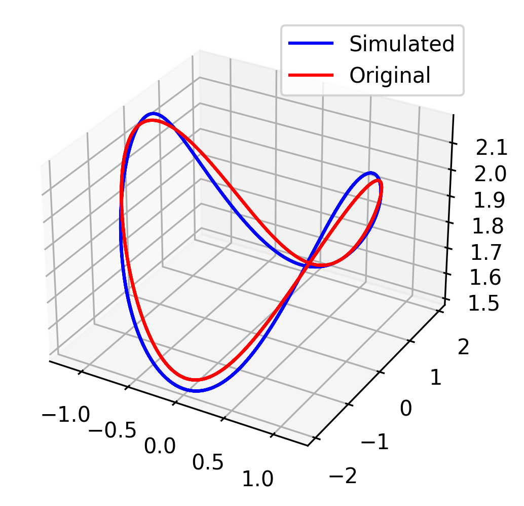
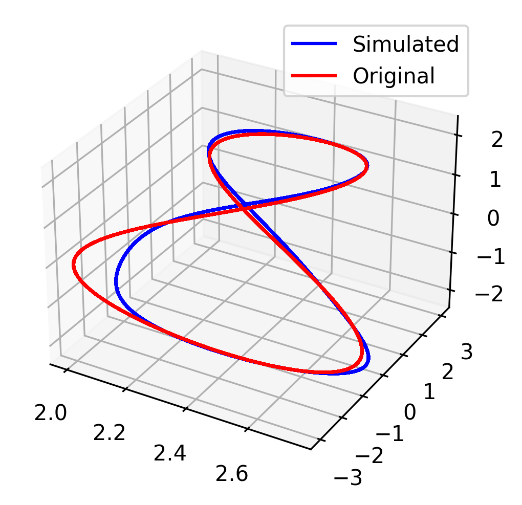
Figure 1: Comparison of the simulated dynamics (blue) and the real trajectory (red) when the initial condition are the points $(1,1,2)$ (top plot) and $(3,2,0)$ (bottom plot).

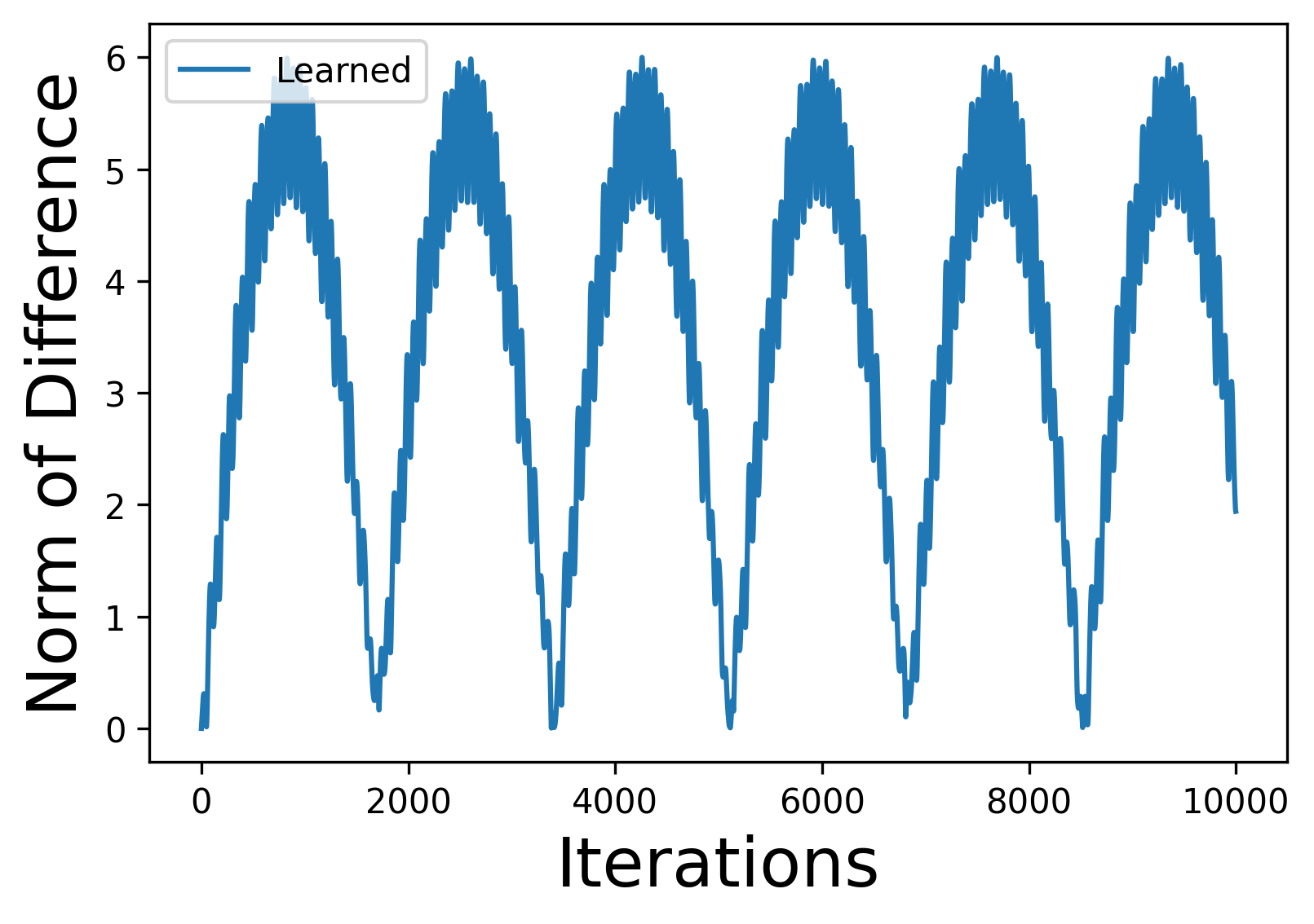
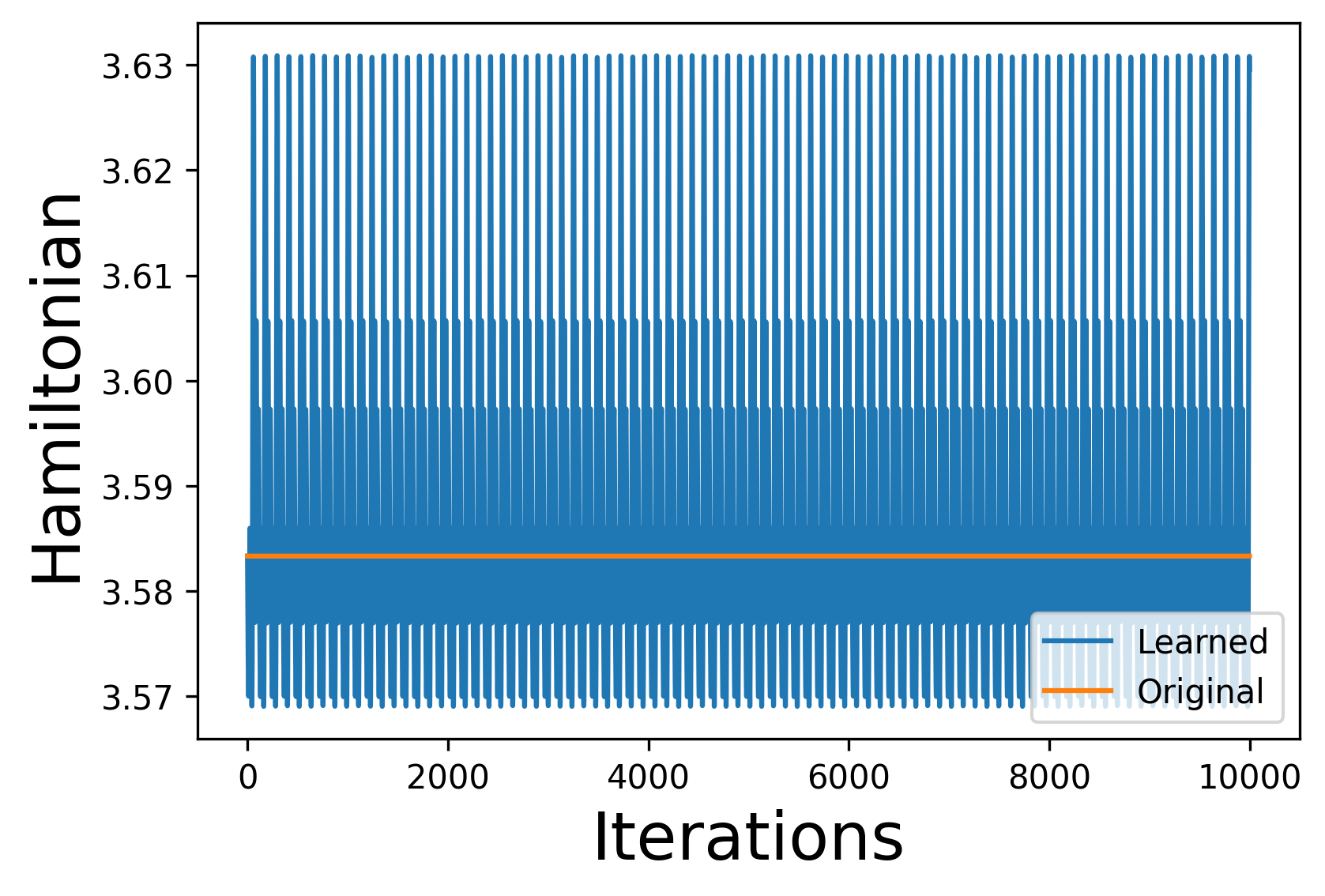
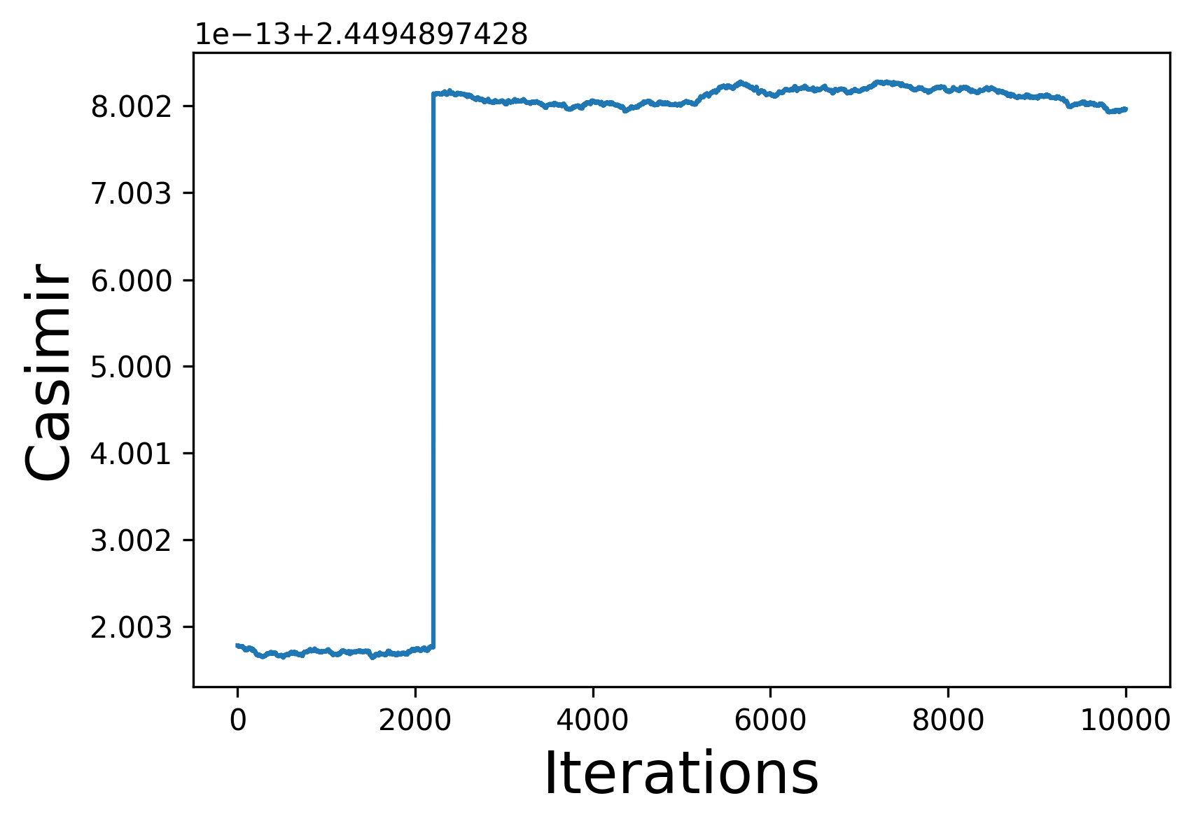
Figure 2: Top: Evolution of the norm of the difference between the simulated and the real trajectories for $10,000$ iterations with stepsize $0.1$. The difference stays bounded due to the conservation of the underlying geometry. Middle: Evolution of the Hamiltonian when evaluated on the simulated trajectory. The Hamiltonian is almost conserved even for very long trajectories. Bottom: Evolution of the Casimir. The Casimir function is conserved up to rounding error.

5 Conclusions and Future Work

In this paper, we delved into the geometric setting presented previously in Vaquero et al. (2023). The framework introduced possesses several properties that make it compelling for the design of Poisson integrators: it fully respects the underlying Poisson geometry and it is highly flexible, making it amenable to various modifications and improvements. Here, we describe a couple of research directions that we plan to pursue.

General Poisson Structures: When the symplectic groupoid is not readily available, several means can be used to approximate it. Two main constructions (Cabrera, 2022) have been proposed to produce local symplectic groupoids that can integrate (locally) any Poisson manifold. An ongoing research direction aims to exploit these constructions to extend the presented framework to any Poisson manifold.

Combination with Data: In some situations, trajectories of the system are available. These trajectories might have been obtained through other (geometric or non-geometric) integrators or might correspond to actual measurements. In these cases, we envision a blended approach that combines both the data and the Hamilton-Jacobi equation. In this fashion, we follow the spirit of PINNS as described by Raissi et al. (2019), designing integrators though finding the Lagrangian submanifold that minimizes an objective function of the type $loss=loss_{HJ}+loss_{data}$. In this objective function $loss_{HJ}$ ensures that the Hamilton-Jacobi equations is satisfied to a certain degree, following the same pattern as in (3). The term $loss_{data}$ would make the Lagrangian submanifold $L$ induce a Poisson transformation that matches the given data.

References

- Abraham and Marsden (1987) Abraham, R. and Marsden, J. (1987). Foundations of Mechanics. Addison Wesley, second edition.
- Arnold (1966) Arnold, V. (1966). Sur la géométrie differentielle des groupes de lie de dimension infinie et ses applications à l’hydrodynamique des fluidsparfaits. Ann. Inst. Fourier, 16, 319–361.
- Cabrera (2022) Cabrera, A. (2022). Generating functions for local symplectic groupoids and non-perturbative semiclassical quantization. Comm. Math. Phys., 395(3), 1243–1296.
- Cosserat (2023) Cosserat, O. (2023). Symplectic groupoids for Poisson integrators. Journal of Geometry and Physics, 186, 104751.
- Coste et al. (1987) Coste, A., Dazord, P., and Weinstein, A. (1987). Groupoï des symplectiques. In Publications du Département de Mathématiques. Nouvelle Série. A, Vol. 2, volume 87 of Publ. Dép. Math. Nouvelle Sér. A, i–ii, 1–62. Univ. Claude-Bernard, Lyon.
- Crainic et al. (2021) Crainic, M., Fernandes, R., and Mărcuţ, I. (2021). Lectures on Poisson Geometry. Graduate Studies in Mathematics. American Mathematical Society.
- Ferraro et al. (2017) Ferraro, S., de León, M., Marrero, J.C., Martín de Diego, D., and Vaquero, M. (2017). On the geometry of the Hamilton-Jacobi equation and generating functions. Arch. Ration. Mech. Anal., 226(1), 243–302.
- Ge (1991) Ge, Z. (1991). Equivariant symplectic difference schemes and generating functions. Phys. D, 49(3), 376–386.
- Goodfellow et al. (2016) Goodfellow, I.J., Bengio, Y., and Courville, A. (2016). Deep Learning. MIT Press, Cambridge, MA, USA. http://www.deeplearningbook.org.
- Hairer et al. (2010) Hairer, E., Lubich, C., and Wanner, G. (2010). Geometric numerical integration, volume 31 of Springer Series in Computational Mathematics. Springer, Heidelberg. Structure-preserving algorithms for ordinary differential equations, Reprint of the second (2006) edition.
- Jin et al. (2023) Jin, P., Zhang, Z., Kevrekidis, I.G., and Karniadakis, G.E. (2023). Learning Poisson systems and trajectories of autonomous systems via Poisson neural networks. IEEE Trans. Neural Netw. Learn. Syst., 34(11), 8271–8283. 10.1109/tnnls.2022.3148734. URL https://doi.org/10.1109/tnnls.2022.3148734.
- Marle (2005) Marle, C.M. (2005). From momentum maps and dual pairs to symplectic and Poisson groupoids. In The breadth of symplectic and Poisson geometry, volume 232 of Progr. Math., 493–523. Birkhäuser Boston, Boston, MA. 10.1007/0-8176-4419-9_17.
- Marsden and Ratiu (1994) Marsden, J. and Ratiu, T. (1994). Introduction to mechanics and symmetry, volume 17. Springer-Verlag, New York. Second edition, 1999.
- McLachlan et al. (2014) McLachlan, R.I., Modin, K., and Verdier, O. (2014). Collective symplectic integrators. Nonlinearity, 27(6), 1525–1542.
- Raissi et al. (2019) Raissi, M., Perdikaris, P., and Karniadakis, G.E. (2019). Physics-informed neural networks: a deep learning framework for solving forward and inverse problems involving nonlinear partial differential equations. J. Comput. Phys., 378, 686–707.
- Sanz-Serna and Calvo (1994) Sanz-Serna, J.M. and Calvo, M.P. (1994). Numerical Hamiltonian problems, volume 7 of Applied Mathematics and Mathematical Computation. Chapman & Hall, London.
- Vaquero et al. (2023) Vaquero, M., Cortés, J., and Martín de Diego, D. (2023). Symmetry preservation in Hamiltonian systems: Simulation and Learning.
- Weinstein (1983) Weinstein, A. (1983). The local structure of Poisson manifolds. J. Differential Geom., 18(3), 523–557. URL http://projecteuclid.org/euclid.jdg/1214437787.
- Zhong and Marsden (1988) Zhong, G. and Marsden, J.E. (1988). Lie-Poisson Hamilton-Jacobi theory and Lie-Poisson integrators. Phys. Lett. A, 133(3), 134–139.