Formation of two singly-ionized Oxygen atoms during the breakup of O₂ driven by an XUV pulse

Abstract

We compute accurate potential energy curves of O₂ up to O${}_{2}^{2+}$ for states that are energetically accessible in the photon energy range 20 to 42 eV. We find the dissociation limits of these states and the atomic fragments to which they dissociate. We use the Velocity Verlet algorithm to account for the nuclear dynamics of O₂ using these computed potential energy curves. Through the use of Monte Carlo simulations which monitor the nuclear motion and electronic structure of the molecule, we obtain kinetic energy release distributions of the O⁺ + O⁺ atomic fragments of O₂ exposed to an XUV pulse in the photon energy range. We compare these theoretical kinetic energy release distributions with results obtained from experiment.

I Introduction

In recent years, the advent of extreme ultraviolet (XUV) laser sources has opened up new avenues for probing ultrafast dynamics in molecular systems with unprecedented temporal and spatial resolution Dudovich et al. (2006). The interaction between XUV photons and molecules initiates complex processes, leading to the generation of highly excited electronic states, molecular fragmentation, and the release of a diverse spectra of kinetic energy. Understanding these processes is not only crucial for advancing fundamental knowledge in molecular physics but also holds significant implications for applications ranging from attosecond science to laser-induced chemistry and biology Lin et al. (2006); Nisoli and Sansone (2009); Miller (2018); Borrego-Varillas et al. (2022).

One of the fundamental challenges in this field is to accurately characterize the kinetic energy release (KER) distributions resulting from the interaction between molecules and laser pulses. These KER distributions provide invaluable insights into the underlying dynamics of molecular fragmentation via bond dissociation pathways. Moreover, precise knowledge of KER distributions is essential for designing and controlling laser-molecule interactions for various technological applications, such as laser-based spectroscopy, molecular imaging, and precision molecular manipulation.

In particular Oxygen, O₂, is of great interest due its significance in biological, chemical and ecological systems, as well as in many other processes Jensen and Ryde (2004); Paterson et al. (2006); Parker (2000). It plays a key role in both the Earth’s atmosphere and all living organisms. The ground state of O₂, namely $X^{3}\Sigma_{g}^{-}$, is in a triplet state between the two open $\pi_{g}$ orbitals. The removal of electrons from the valence orbitals via single-photon ionization or Auger decay produces an array of ionic states. Computing the energies of these various states can be complex due to the open-shell configuration, especially in the cases where an electron is removed from an inner valence orbital.

Motivated by these considerations, this paper presents a theoretical study aimed at calculating the KER distributions of O₂ molecules subjected to intense XUV laser pulses. We will leverage state-of-the-art quantum-classical hybrid techniques, including ab initio electronic structure calculations Mountney et al. (2023) and classical molecular dynamics simulations. In Section II, we outline our methods for producing KER distributions of O₂ when an XUV pulse is applied to the molecule. In Section III, we outline the experimental set up for the same interaction. Then in Section IV, we plot and discuss our results using the techniques described above. In particular, we consider both a low and high intensity XUV pulse in the photon energy range 20 to 42 eV. We will outline the key features of our KER distributions, as well as the pathways through various ionic states of O₂ that lead to the spectra observed.

II Theoretical method

In order to obtain KER distributions of O₂, we will run Monte Carlo simulations using a quantum-classical hybrid method which will model the interaction between the O₂ molecule and the XUV pulse. We apply the Born-Oppenheimer approximation Born and Oppenheimer (1927) to separate the nuclear and electronic motion of the molecule. The electronic structure is modelled quantum mechanically, which is described in Section II.1. We solve for the nuclear motion classically using the Hamiltonian for a two-body system using quantum mechanically-obtained potential energy curves (PECs). In Section II.2, we discuss how we use the two-body problem in the context of a diatomic molecule and in Section II.3 we describe how we obtain the PECs. Then, in Section II.5 we discuss how we calculate the internuclear distance and momentum at each time step of the Monte Carlo simulations, as well as how we initially sample them in Section II.6. If the molecule dissociates into atomic fragments during the Monte Carlo simulations, we calculate the velocities of these atoms at the point of dissociation. At the end of the simulations, we can then plot the velocities of the O⁺ + O⁺ dissociated fragments in a KER distribution. In Section II.4, we outline our criteria for molecule to dissociate.

II.1 Electronic structure

In order to model the motion of the electrons in the molecule, we must be able to accurately define the wavefunctions of both the bound and continuum electrons. The wavefunctions of the bound orbital electrons are calculated using the Hartree-Fock (HF) method in the framework of the quantum chemistry package MOLPRO Werner et al. (2012). Using these wavefunctions, we then solve a system of HF equations Mountney et al. (2022); Banks et al. (2017) to find the wavefunction of an electron which has escaped to the continuum via either single-photon ionization or Auger Decay. Using these continuum wavefunctions, as well as the wavefunctions of the bound electrons, we can calculate the photoionization cross sections and Auger rates for a transition to occur. We express the continuum and bound state wavefunctions using a single center expansion (SCE) Demekhin et al. (2011); Banks et al. (2017)

$$\psi(\vec{r})=\sum_{lm}\frac{P_{lm}(r)Y_{lm}(\theta,\phi)}{r}$$ (1)

where $l,m$ are the angular momentum and magnetic quantum numbers respectively, $Y_{lm}$ is a spherical harmonic and $P_{lm}$ is the radial part of the wavefunction. Note that we fully account for the Coulomb potential. Then, the photoionization cross section for an electron transitioning from an initial orbital $\psi_{i}$ to a final continuum orbital $\psi_{\epsilon}$ is given by Banks et al. (2020); Sakurai (1994)

$$\sigma_{i\rightarrow\epsilon}=\frac{4}{3}\alpha\pi^{2}\omega N_{i}\sum_{M=-1,0,1}\absolutevalue{D^{M}_{i\epsilon}}^{2},$$ (2)

where $\alpha$ is the fine-structure constant, $\omega$ the photon energy, $N_{i}$ the occupation number of orbital $i$ and $M$ the polarization of the photon. In the length gauge the dipole matrix element, $D^{M}_{i\epsilon}$, is given by the following

$$D^{M}_{i\epsilon}=\int\psi^{*}_{\epsilon}(\textbf{r})\psi_{i}(\textbf{r})\sqrt{\frac{4\pi}{3}}Y_{1M}(\theta,\phi)d\textbf{r}.$$ (3)

The general expression for the Auger Rate is given by Banks et al. (2020); Pauli (2000)

$$\Gamma=\overline{\sum}2\pi\absolutevalue{\mathcal{M}}^{2}=\overline{\sum}2\pi\absolutevalue{\bra{\Psi_{fin}}H_{I}\ket{\Psi_{init}}}^{2},$$ (4)

where $\overline{\Sigma}$ denotes a summation over the final states and an average over the initial states. $H_{I}$ is the interaction Hamiltonian and $\ket{\Psi_{init}}$, $\ket{\Psi_{fin}}$ are the initial and final wavefunctions of all electrons in the initial and final molecular state, respectively. At each time step of the Monte Carlo simulations, we use these probabilities to determine if a transition occurs. This is discussed in more detail in Section II.7.

II.2 Two body Hamiltonian for nuclear motion

The nuclear motion of the molecule is solved classically. In classical mechanics, the total energy of a two-body system with potential energy $U(\textbf{r})$ is

$$\begin{split}E&=\frac{1}{2}m_{1}\dot{\textbf{x}}_{1}^{2}+\frac{1}{2}m_{1}\dot{\textbf{x}}_{2}^{2}+U(\textbf{r})\\ &=\frac{1}{2}(m_{1}+m_{2})\dot{\textbf{R}}^{2}+\frac{1}{2}\mu\dot{\textbf{r}}^{2}+U(\textbf{r}),\end{split}$$ (5)

where $m_{1},m_{2}$ are the masses of the two nuclei and

$$\begin{split}&\mu=\frac{m_{1}m_{2}}{m_{1}+m_{2}}\\ &\textbf{x}_{1}=\frac{\mu}{m_{1}}\textbf{r}\implies\dot{\textbf{x}}_{1}=\frac{\mu}{m_{1}}\dot{\textbf{r}}\\ &\textbf{x}_{2}=-\frac{\mu}{m_{2}}\textbf{r}\implies\dot{\textbf{x}}_{2}=-\frac{\mu}{m_{2}}\dot{\textbf{r}}\\ &\textbf{r}=\textbf{x}_{1}-\textbf{x}_{2}\\ &\textbf{R}=\frac{m_{1}}{m_{1}+m_{2}}\textbf{x}_{1}+\frac{m_{2}}{m_{1}+m_{2}}\textbf{x}_{2}.\end{split}$$ (6)

Here, $R=\absolutevalue{\textbf{R}}$ is the internuclear distance of the molecule. The potential energy will be calculated using quantum mechanically-obtained PECs for all relevant states of O₂.

II.3 Computation of potential energy curves

The electronic configuration of the ground state of O₂ is ($1\sigma_{g}^{2}$, $1\sigma_{u}^{2}$, $2\sigma_{g}^{2}$, $2\sigma_{u}^{2}$, $3\sigma_{g}^{2}$, $1\pi_{ux}^{2}$, $1\pi_{uy}^{2}$, $1\pi_{gx}^{1}$, $1\pi_{gy}^{1}$). As we can see, the ground state is in a triplet state between the $1\pi_{g}$ orbitals. We will compute PECs of O₂ up to O${}_{2}^{2+}$ ionic states which are energetically accessible via single-photon photoionization or Auger decay within the photon energy range 20 to 42 eV. This photon energy range is sufficient to ionize electrons up to the inner valence orbital $2\sigma_{g}$. To obtain accurate PECs, we use the complete active space self-consistent field (CASSCF) method, followed by the multireference configuration interaction (MRCI) method in MOLPRO Werner et al. (2012). When using MOLPRO, we employ the augmented Dunning correlation consistent quadruple valence basis set (aug-cc-pVQZ) Dunning (1989). We use 12 active orbitals in the active space of our PEC calculations, with 3 of those being virtual orbitals (namely $3\sigma_{u}$, $4\sigma_{g}$ and $4\sigma_{u}$). In cases where a state possessed equal symmetries to states lower in energy, we performed state-averaged MRCI calculations. For some states, convergence could not be reached using the MRCI method, and hence in these cases only the CASSCF method was used. We found the equilibrium distance of the ground state of O₂ to be equal to $1.205$ Å = 2.28 a.u., in agreement with Refs. Bytautas et al. (2010); Weast (1985). To generate smooth PECs, we compute the energy of the states every $0.05$ Å. In Fig. 1, we compare our PECs with the theoretical PECs obtained in Refs. Magrakvelidze et al. (2012); Lundqvist et al. (1996); Larsson et al. (1990).

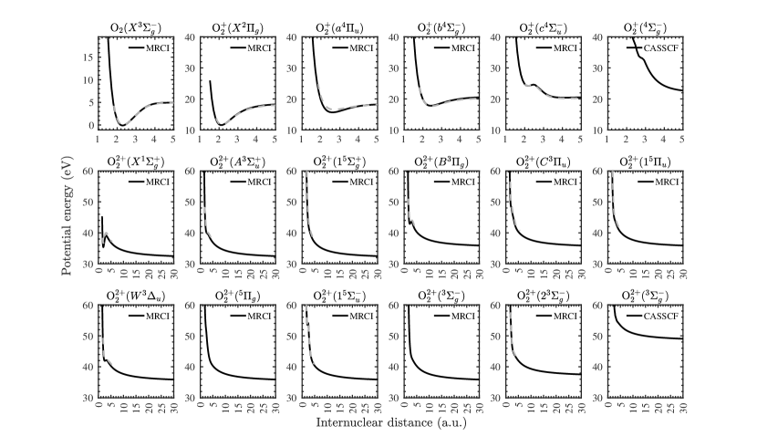
Figure 1: Potential energy curves of O₂, O${}_{2}^{+}$ and O${}_{2}^{2+}$, compared with Refs. Magrakvelidze et al. (2012); Lundqvist et al. (1996); Larsson et al. (1990) (gray dashed lines).

II.4 Dissociation of molecular states

When the internuclear distance between two atoms in a diatomic molecule reaches a certain threshold, the interaction potential between the atoms becomes negligible and hence we can consider the atoms separately. However, the distance at which dissociation occurs is relatively ambiguous. In our calculations, we assume that this dissociation occurs when the energy of a molecular state reaches 99% of its dissociation energy. We found this was a reasonable criteria for dissociation as all the PECs exhibited purely repulsive behaviour beyond this point.
To find the atomic fragments to which the molecular states of O₂ dissociate into, we compared the dissociation energies of the molecular states with energies of various atomic states. The dissociation energy of a molecular state should be equal to the sum of the energies of its atomic fragments. We then verified our findings with the literature Magrakvelidze et al. (2012); Hikosaka et al. (2003). We computed the atomic energies again using MRCI and the aug-cc-pVQZ basis set in MOLPRO. In Table 1 we show the dissociation fragments for all states used in our calculations, along with their respective energies.

Atomic fragments	Sum of energies of atomic fragments
	Our work (eV)	Other work (eV)
O(${}^{3}P$)+O(${}^{3}P$)	5.0	5.0 Magrakvelidze et al. (2012)
O(${}^{3}P$)+O+(${}^{4}S$)	18.5	18.8 Magrakvelidze et al. (2012)
O(${}^{1}D$)+O+(${}^{4}S$)	20.5	20.7 Magrakvelidze et al. (2012)
O(${}^{3}P$)+O+(${}^{2}P$)	22.3	23.8 Hikosaka et al. (2003)
O+(${}^{4}S$)+O+(${}^{4}S$)	31.6	32.4 Magrakvelidze et al. (2012)
O+(${}^{4}S$)+O+(${}^{2}D$)	35.0	35.7 Magrakvelidze et al. (2012)
O+(${}^{4}S$)+O+(${}^{2}P$)	36.6	37.3 Magrakvelidze et al. (2012)
O+(${}^{2}D$)+O+(${}^{2}D$)	48.1*	39.0 Magrakvelidze et al. (2012)

Table 1: Atomic dissociation fragments of O₂, O${}_{2}^{+}$ and O${}_{2}^{2+}$ with their respective dissociation energies compared with other theoretical work Magrakvelidze et al. (2012); Hikosaka et al. (2003). *Calculated using only the CASSCF method due to lack of convergence in the MRCI method, as mentioned in Section II.3.

II.5 Algorithm for time propagating the nuclei

When accounting for the nuclear dynamics of a diatomic molecule, we are specifically accounting for the relative velocity and distance between the atoms, i.e. the internuclear distance and momentum. To track the internuclear distance and velocity, we employ the Velocity-Verlet algorithm Verlet (1967). The algorithm calculates the distance and velocity at each time step recursively. It is given by the following equations

$$\begin{split}&R_{n+1}=R_{n}+v_{n}\Delta t+\frac{1}{2\mu}f_{n}(\Delta t)^{2}\\ &v_{n+1}=v_{n}+\frac{1}{2\mu}(f_{n+1}+f_{n})(\Delta t),\end{split}$$ (7)

where $\mu,\Delta t,R,v,f$ are the reduced mass of the molecule, time step, internuclear distance, velocity and force, respectively. In our case, we calculate the force by taking the negative of the derivative of the potential with respect to distance. In other words,

$$\begin{split}f_{n}&=-\frac{dU(R_{n})}{dR}\\ f_{n+1}&=-\frac{dU(R_{n+1})}{dR},\end{split}$$ (8)

where $U$ is the potential energy of the current state, which is equal to the potential in Eq. (5). If a transition has occurred in that time step, we use the potential of the new state.

II.6 Sampling the initial conditions of the nuclei

We sample the initial internuclear distance and momentum of the molecule in two steps. Firstly, we sample the initial internuclear distance using importance sampling Rubinstein and Froese (2007). This is weighted by the Morse wave function Frank et al. (2000) of the ground state of neutral O₂, given by

$$\begin{split}\psi_{j,0}(r)&=N_{j,0}e^{-\xi/2}\xi^{j}L_{0}^{2j}(\xi)\\ N_{j,0}&=\frac{\beta j}{\Gamma(2j+1)}\\ \xi&=(2j+1)e^{-\beta x}\end{split}$$ (9)

where $x=r-R$ is the displacement of the internuclear distance from equilibrium ($R$ is the equilibrium distance) and $\Gamma$ is the Gamma function. The coefficient $\beta$ is related to the harmonic vibrational frequency $\omega_{e}$ by the following expression

$$\omega_{e}=\beta\sqrt{\frac{2D_{e}}{\mu}},$$ (10)

where $D_{e}$ is the dissociation energy and $\mu$ the reduced mass of the molecule. Once we have obtained the initial internuclear distance, we perform importance sampling of the initial momentum weighted by the Wigner function Frank et al. (2000) of the ground state of neutral O₂ at the sampled internuclear distance. The Wigner function is given by

$$W(\psi_{j,0}|r,p)=\frac{2}{\pi\hbar\Gamma(2j)}\xi^{2j}K_{-2ip/\beta\hbar}(\xi)$$ (11)

where $K_{-2ip/\beta\hbar}(\xi)$ are the modified Bessel functions of the third kind Slater et al. (1965). In Fig. 2, we plot the distributions of the Morse wave function and the Wigner function for O₂.

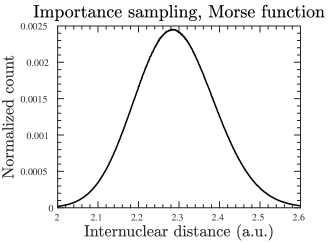
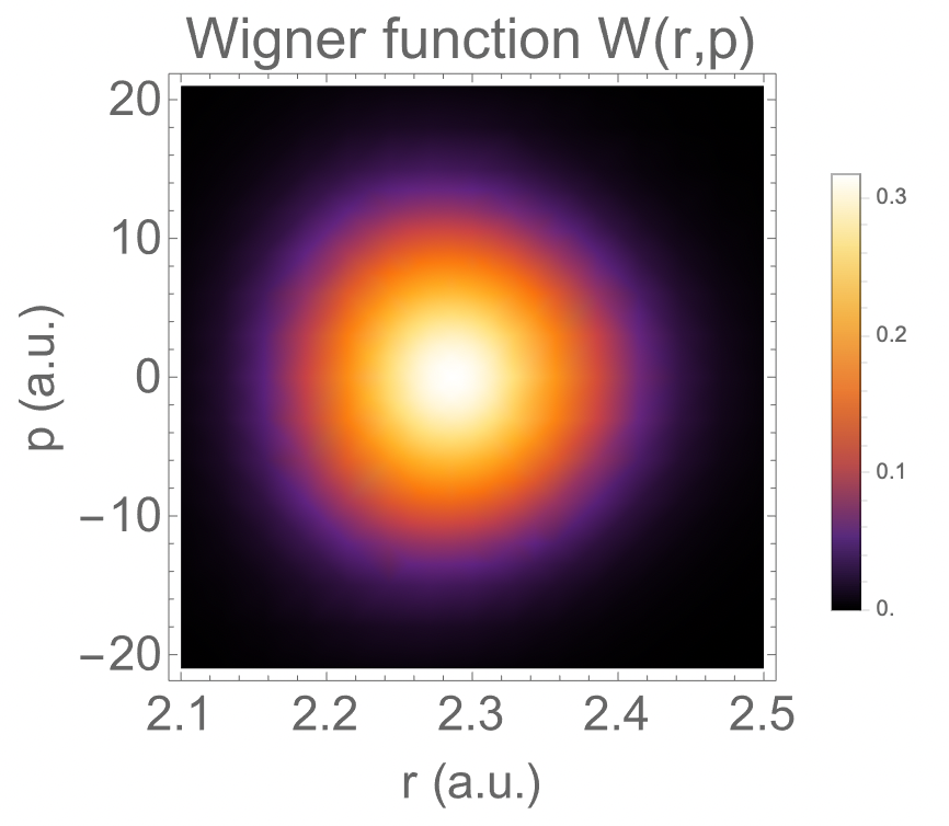
Figure 2: Distributions used in importance sampling. Top: distribution of internuclear distances using the Morse function for the ground state of O₂. Bottom: distribution of internuclear distance and momenta using the Wigner function for the ground state of O₂.

II.7 Monte Carlo techniques

Using the algorithm outlined in the previous section, we will run Monte-Carlo simulations to find the various pathways the molecule can take and the kinetic energy of the dissociative atomic fragments. As mentioned earlier, these simulations utilise atomic and molecular single-photon photoionization cross sections and Auger rates, outlined in Eqns. (2) and (4), to predict transitions to other states. At each time step of the Monte-Carlo simulation, we take all of the transitions available to the current state and calculate their transition rates. For atomic states, the transition rates are calculated as follows

$$\begin{split}\omega_{\alpha i}(t)&=\sigma_{\alpha i}J(t)\ \ \ \text{Photoionization}\\ \omega_{\alpha i}(t)&=\Gamma_{\alpha i}\ \ \ \ \ \ \ \ \text{Auger decay},\end{split}$$ (12)

where $\omega_{\alpha i}$ is the transition rate of the $i$th transition from configuration $\alpha$, $\sigma_{\alpha i}(r)$ is the photoionization cross section for a certain transition, $J(t)$ the photon flux at time $t$ and $\Gamma_{\alpha i}$ the Auger rate. For molecular states, the transition rates change with respect to the internuclear distance of the molecule. Hence the transition rates in this case are calculated as follows

$$\begin{split}\omega_{\alpha i}(t,R)&=\sigma_{\alpha i}(R)J(t)\ \ \ \text{Photoionization}\\ \omega_{\alpha i}(t,R)&=\Gamma_{\alpha i}(R)\ \ \ \ \ \ \ \ \text{Auger decay},\end{split}$$ (13)

where $R$ is the internuclear distance of the molecule. Then, we use the fact that the population of the species follows an exponential decay law, i.e.

$$P=P_{0}e^{-\omega_{\alpha i}t},$$ (14)

where $P$ is the population at time $t$ and $P_{0}$ is the initial population at time $t=0$. Hence if we select a random value of $P$ such that $\frac{P}{P_{0}}<1$, the corresponding time for this transition is

$$t_{i_{\alpha}}(t)=-\frac{\log{\frac{P}{P_{0}}}}{\omega_{\alpha i}}.$$ (15)

We use this method to find transition times for each of the transitions from our current states. If any of these transition times are smaller than the time step (in our case we use 0.01 fs as we found the results converged using time steps any smaller), then we advance time by $t_{i_{\alpha}}$ and move to the final state in the transition. If none of the transition times are smaller than the time step, then we advance time by the time step. After this step, we then perform the Velocity-Verlet algorithm to determine the internuclear distance and velocity for the next time step. If a transition has occurred, then we use the PEC of this new state to calculate the force.

III Experimental setup

The measurement on O₂ was performed with the reaction microscope (REMI) endstation Meister et al. (2020); Schmid et al. (2019) at the Free electron laser (FEL) in Hamburg (FLASH2) Ackermann et al. (2007); Faatz et al. (2016). The setup allows one to analyze ionization and fragmentation processes and to measure particles of the same event in a coincidence. In the ultra-high vacuum ($\approx$ 10-11 mbar) detection chamber a supersonic gas jet is crossed at 90^∘ with the focused XUV FEL beam. Electrons and ions which are generated during ionization are guided onto spatial and time sensitive detectors by means of E and B-fields. Time-of-flight information and impact position of a particle allows one to back calculate the particles momentum vector at the instant of ionization. Momentum conservation between particles of the same laser pulse can be used to sort out all fragments stemming from the same ionization or fragmentation event.

For the experiment the FEL was operated in a pattern of 38 pulses temporally spaced by approximately 13 $\mu$s (77 kHz), repeating in a 10 Hz period. This results in an effective repetition rate of 380 Hz. Thanks to the variable gap undulators the photon energy was easily and repeatedly scanned between 20 eV and 42 eV in steps of 0.2 eV. Within this range the pulse energy, measured by the gas monitor detector (GMD) in the experimental hall, varied between 10 and 30 $\mu$J while about a fourth of this value is delivered on target. As the FEL pulse energy and other beam parameters change systematically with the photon energy, the experimental O⁺-ion yield in Figure 3 is normalized with the simultaneously recorded H${}_{2}^{+}$ -yield from residual H₂ gas in the REMI chamber. This procedure is done by taking the total absorption cross section of H₂ into account Samson and Haddad (1994).

The electric field strength was set to about 16 Vcm^-1 such that Coulomb exploding O⁺ pairs are detected in a $4\pi$ solid angle. The nozzle of the supersonic gas source was cooled to roughly -158 ^∘C, just above the condensation point of O₂ in order prevent clogging. Cryogenic temperatures were chosen to reduce internal energy and to decrease momentum spread of the oxygen molecules in the jet.

IV Results

Below are our results using the methods outlined above to find the KER distributions of the O⁺ + O⁺ atomic fragments of O₂ when we apply an XUV laser pulse to the molecule. The photon energies of the laser pulse range between 20 and 42 eV in increments of 1 eV. We consider intensities of the XUV pulse of $5\times 10^{12}$ W/cm² and $5\times 10^{14}$ W/cm² and a full-width at half maximum (FWHM) of 100 fs. We measured the Monte Carlo simulations over a span of 1500 fs: 500 fs before the peak of the laser pulse and 1000 fs after. We found convergence in our results taking this length of time. At each photon energy, we performed 5 million Monte Carlo simulations.

Note that in our theoretical calculations, we do not utilise excited states of O₂. This is because we do not possess accurate probabilities to transition to excited states. However, we will see that our KER distributions still include the majority of features that we see in experiment. This is due to coupling effects between excited and non-excited states, as well as the fact that the excited states of O${}_{2}^{+}$ ionize to non-excited O${}_{2}^{2+}$ that we do include in our calculations.

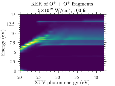
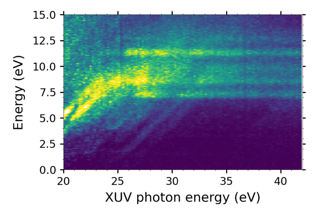
Figure 3: Kinetic energy release spectra for O⁺ + O⁺ fragments with respect to the photon energy. (a) The theoretical results at the end of the Monte Carlo simulations with a laser intensity of $5\times 10^{12}$ W/cm² and full width at half maximum of 100 fs. (b) Experimental results.

In Fig. 3(a), we plot the KER distributions of the O⁺ + O⁺ fragments at the end of the simulations with respect to the photon energy. At each photon energy, we have normalized the distributions by dividing by the number of simulations that ended with O⁺ + O⁺ fragments. We used a weak laser pulse intensity of $5\times 10^{12}$ W/cm² and a FWHM of 100 fs. We compare this with the KER distribution from experiment in Fig. 3(b). As we can see, in both cases there is an initial peak of 5 eV kinetic energy at 20 eV photon energy, which increases up to 8 eV at 25 eV photon energy. From 25 eV photon energy onwards, we observe different peaks in the kinetic energy spectra, ranging from 7 to 13 eV. This spectra then continues from 25 to 42 eV, giving the straight lines that we see. In our theoretical results we do not observe the peak at approximately 11 eV that we see in experiment. This is due to the exclusion of excited states in our calculations.

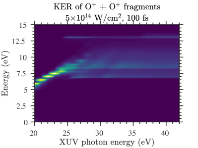
Figure 4: Same as Fig. 3(a) for but a laser intensity of $5\times 10^{14}$ W/cm².

In Fig. 4, we again plot the KER distributions of the O⁺ + O⁺ fragments, but now with a much stronger intensity of $5\times 10^{14}$ W/cm². The main features are the same as in Fig. 3(a), but the concentration of spectra differ. We will see that this is due to the difference in the proportion of various pathways leading to the formation of the O⁺ + O⁺ fragments.

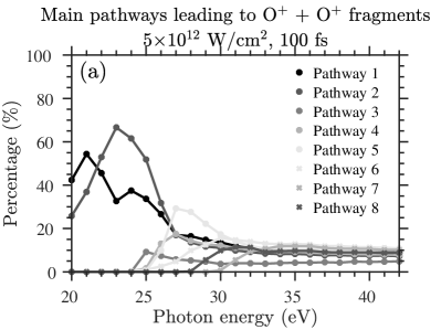
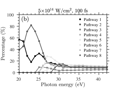
Figure 5: Contributions of the 8 main pathways leading to O⁺ + O⁺ fragments as a percentage with respect to photon energy. The FWHM of the laser pulse is 100 fs and the laser intensity is (a) $5\times 10^{12}$ W/cm² (b) $5\times 10^{14}$ W/cm².

In order to understand the features of the KER distributions, let use look at the main pathways leading to O⁺ + O⁺ fragments. These pathways are:

$$\begin{split}&\text{Pathway 1: O}_{2}\rightarrow\text{O}_{2}^{+}(a^{4}\Pi_{u})\rightarrow\text{O}_{2}^{2+}(1^{5}\Sigma_{g}^{+})\\ &\text{Pathway 2: O}_{2}\rightarrow\text{O}_{2}^{+}(a^{4}\Pi_{u})\rightarrow\text{O}_{2}^{2+}(A^{3}\Sigma_{u}^{+})\\ &\text{Pathway 3: O}_{2}\rightarrow\text{O}_{2}^{+}(c^{4}\Sigma_{u}^{-})\rightarrow\text{O}_{2}^{2+}(C^{3}\Pi_{u})\\ &\text{Pathway 4: O}_{2}\rightarrow\text{O}_{2}^{+}(a^{4}\Pi_{u})\rightarrow\text{O}_{2}^{2+}(W^{3}\Delta_{u})\\ &\text{Pathway 5: O}_{2}\rightarrow\text{O}_{2}^{+}(b^{4}\Sigma_{g}^{-})\rightarrow\text{O}_{2}^{2+}(1^{5}\Pi_{u})\\ &\text{Pathway 6: O}_{2}\rightarrow\text{O}_{2}^{+}(a^{4}\Pi_{u})\rightarrow\text{O}_{2}^{2+}(1^{5}\Pi_{u})\\ &\text{Pathway 7: O}_{2}\rightarrow\text{O}_{2}^{+}(X^{2}\Pi_{g})\rightarrow\text{O}_{2}^{2+}(W^{3}\Delta_{u})\\ &\text{Pathway 8: O}_{2}\rightarrow\text{O}_{2}^{+}(X^{2}\Pi_{g})\rightarrow\text{O}_{2}^{2+}(A^{3}\Sigma_{u}^{+}),\end{split}$$

where O₂ is the ground state, namely $X^{3}\Sigma_{g}^{-}$. Looking at the PECs in Fig. 1, we can these that all of these O${}_{2}^{2+}$ states are repulsive. Since these states do not possess a potential well, the internuclear distance will explode rapidly, causing them to dissociate to O⁺ + O⁺ fragments. In Fig. 5, we plot the percentage that each pathway contributes to the number of simulations that lead to O⁺ + O⁺ fragments, with respect to the photon energy. Up to 25 eV photon energy, we can see that only pathways 1 and 2 are responsible for the O⁺ + O⁺ KER distribution. From 25 eV photon energy onwards, all these pathways listed above contribute roughly the same to the O⁺ + O⁺ KER distribution. In Fig. 5(b), we see a much larger contribution from pathway 2 than Fig. 5(a) between 20 and 25 eV photon energy. From 25 eV photon energy onwards, the difference between Fig. 5(a) and (b) is negligible. This results in a larger concentration of kinetic energy for the lower kinetic energies in Fig. 4 and hence the appearance of a lower concentration of spectral lines between 25 and 42 eV when compared with Fig. 3(a).

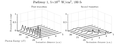
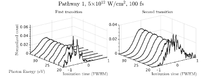
Figure 6: Distributions of ionization distances (above) and times (below) for pathway 1. The first transition is from O₂ to O${}_{2}^{+}$. The second transition is from O${}_{2}^{+}$ to O${}_{2}^{2+}$.

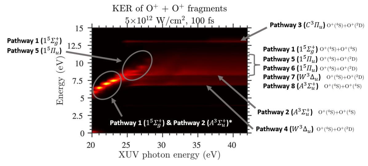
Figure 7: Annotated kinetic energy release spectra of O⁺ + O⁺ fragments, explaining which pathways give rise to which features.

In Fig. 6, we plot the distributions of ionization times and distances for pathway 1. The first transition is O${}_{2}(X^{3}\Sigma_{g}^{-})$ $\rightarrow$ O${}_{2}^{+}(a^{4}\Pi_{u})$, and the second transition is O${}_{2}^{+}(a^{4}\Pi_{u})$ $\rightarrow$ O${}_{2}^{2+}(1^{5}\Sigma_{g}^{+})$. The first transition is centred around the equilibrium distance of 2.28 a.u. for all photon energies. This is true of all pathways since our initial internuclear distance is sampled around this distance, see Fig. 2. For the second transition, we can see that the distribution is centred around larger internuclear distances for smaller photon energies. As we increase the photon energy, the distribution centres around smaller internuclear distances. From around 27 eV onwards, the distribution is centred around the equilibrium distance. This will help us explain the shape of the KER distribution. From Eq. (7), we can see that the velocity is determined by the force, i.e. the derivative of the PEC at the current internuclear distance. Let us look at the PEC of the O${}_{2}^{2+}$ state involved in pathway 1, namely O${}_{2}^{2+}(1^{5}\Sigma_{g}^{+})$. From Fig. 1, we can see that at larger internuclear distances, the slope of the PEC is very shallow and hence the velocity gained will be smaller. At smaller distances, the PEC is very steep and hence the velocity gained will be larger. This explains why we see smaller kinetic energy for smaller photon energies, increasing up to a constant amount at larger photon energies. We can explain the other features of the KER distributions through similar analysis of the other main pathways. In Fig. 7, we outline which pathways give rise to which features of the KER distribution. Beside each pathway, we give the atomic fragments to which the O${}_{2}^{2+}$ states in these pathways dissociate.

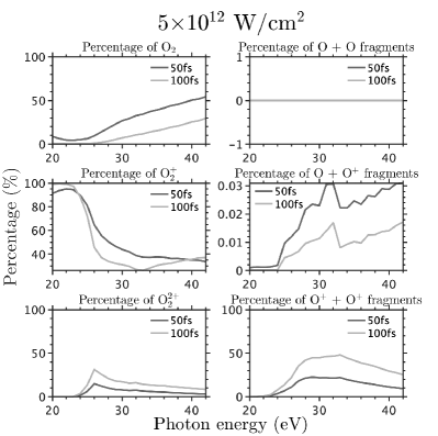
Figure 8: Percentages of each final atomic and molecular ionic states with respect to photon energy.

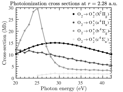
Figure 9: Photoionization cross sections to transition from O₂ to O${}_{2}^{+}$ at the equilibrium distance of O₂, $r=2.28$ a.u. with respect to photon energy.

In Fig. 8, we plot the percentages of all possible final ionic states, molecular and atomic, at the end of the Monte Carlo simulations. We show results for a laser intensity of $5\times 10^{12}$ W/cm² and FWHMs of 50 and 100 fs. Firstly, we can see that the percentage of O₂ is larger for 50 fs than for 100 fs. Clearly, since the pulse is shorter it less likely that photoionization will occur and hence the population of O₂ at the end of the simulation will be larger. Similarly, the percentage of O${}_{2}^{2+}$ and O⁺ + O⁺ fragments is larger for 100 fs. To understand why the percentage of O₂ increases as the photon energy increases, we need to consider the photoionization cross sections. In Fig. 9, we plot the photoionization cross sections to transition from O₂ to O${}_{2}^{+}$ at the equilibrium distance with respect to the photon energy. As we can see, in all cases the cross section decreases as the photon energy increases. Hence, as the photon energy increases it is less likely for ionization from O₂ to occur. Furthermore, we do not see any O + O fragments since the ground state of O₂ possesses a very large potential well, see Fig. 1. This makes it extremely difficult for the internuclear distance to explode and hence cause dissociation. Similarly, we see very little O + O⁺ fragments since most of the O${}_{2}^{+}$ states possess a potential well around the equilibrium distance. Finally, we can see that the percentage of O${}_{2}^{+}$ is very large up to 25 eV, while the percentage of O${}_{2}^{2+}$ and O⁺ + O⁺ fragments is very small up to this point. After 25 eV, the percentage of O${}_{2}^{+}$ sharply decreases while he percentage of O${}_{2}^{2+}$ and O⁺ + O⁺ increases. This is because at smaller photon energies, the internuclear distance must be large for a transition from O${}_{2}^{+}$ to O${}_{2}^{2+}$ to occur. This can be seen in Fig. 6. As previously mentioned, most O${}_{2}^{+}$ states possess a potential well and hence it is unlikely for the internuclear distance to reach larger values. As the photon energy increases beyond 25 eV, the internuclear distances for a transition from O${}_{2}^{+}$ to O${}_{2}^{2+}$ to occur decreases. It is more likely for the internuclear distance to be in this desired range and hence the percentage of O${}_{2}^{2+}$ and O⁺ + O⁺ increases while the percentage of O${}_{2}^{+}$ decreases.

V Conclusion

In conclusion, we have shown our techniques to account for both the nuclear dynamics and electronic structure of a diatomic molecule when it is exposed to a laser pulse. We have obtained potential energy curves for states of O₂ up to O${}_{2}^{2+}$, and then used them to calculate the internuclear distance and momentum of the molecule at any point in time during the interaction. Moreover, we have described how we use this nuclear motion algorithm, along with transition probabilities that we calculate, to run Monte Carlo simulations to find the results of applying an XUV pulse to O₂. We have discussed the features of the kinetic energy release distributions of the O⁺ + O⁺ fragments of these simulations, as well as the most frequent pathways that lead to these fragments. We verified our findings using experimental data. Finally, we have explained how the shapes of the PECs and the transition probabilities give rise to various ratios of final atomic and molecular ionic states with respect to the photon energy.

VI Acknowledgements

The authors A. E. and M. M. acknowledge the use of the UCL Myriad High Throughput Computing Facility (Myriad@UCL), and associated support services, in the completion of this work. A. E. acknowledges the Leverhulme Trust Research Project Grant No. 2017-376. M. M. acknowledges funding from the EPSRC project 2419551.

References

- Dudovich et al. (2006) N. Dudovich, O. Smirnova, J. Levesque, Y. Mairesse, M. Yu Ivanov, D. M. Villeneuve, and P. B. Corkum, “Measuring and controlling the birth of attosecond XUV pulses,” Nat. Phys 2, 781–786 (2006).
- Lin et al. (2006) C. D. Lin, X. M. Tong, and T. Morishita, “Direct experimental visualization of atomic and electron dynamics with attosecond pulses,” J. Phys. B At. Mol. Opt. Phys. 39, S419 (2006).
- Nisoli and Sansone (2009) M. Nisoli and G. Sansone, “New frontiers in attosecond science,” Progress in Quantum Electronics 33, 17–59 (2009).
- Miller (2018) J. L. Miller, “An attosecond view of electron–nuclear coupling,” Physics Today 71, 20–21 (2018), https://pubs.aip.org/physicstoday/article-pdf/71/6/20/10120949/20_1_online.pdf .
- Borrego-Varillas et al. (2022) R. Borrego-Varillas, M. Lucchini, and M. Nisoli, “Attosecond spectroscopy for the investigation of ultrafast dynamics in atomic, molecular and solid-state physics,” Reports on Progress in Physics 85, 066401 (2022).
- Jensen and Ryde (2004) K. P. Jensen and U. Ryde, “How O2 binds to heme: reasons for rapid binding and spin inversion,” J. Biol. Chem. 279, 14561–14569 (2004).
- Paterson et al. (2006) M. J. Paterson, O. Christiansen, F. Jensen, and P. R. Ogilby, “Overview of theoretical and computational methods applied to the oxygen-organic molecule photosystem,” Photochem. Photobiol. 82, 1136–1160 (2006), https://onlinelibrary.wiley.com/doi/pdf/10.1562/2006-03-17-IR-851 .
- Parker (2000) D. H. Parker, “Laser photochemistry of molecular oxygen,” Accounts of Chemical Research, Acc. Chem. Res. 33, 563–571 (2000).
- Mountney et al. (2023) M. E. Mountney, T. C. Driver, A. Marinelli, M. F. Kling, J. P. Cryan, and A. Emmanouilidou, “Streaking single-electron ionization in open-shell molecules driven by x-ray pulses,” Phys. Rev. A 107, 063111 (2023).
- Born and Oppenheimer (1927) M. Born and R. Oppenheimer, “Zur quantentheorie der molekeln,” Annalen der Physik 389, 457–484 (1927).
- Werner et al. (2012) H.-J. Werner, P. J. Knowles, G. Knizia, F. R. Manby, and M. Schütz, “MOLPRO: a general-purpose quantum chemistry program package,” M. WIRE: Comput. Mol. Sci. 2, 242 (2012).
- Mountney et al. (2022) M. Mountney, G. P. Katsoulis, S. H. Møller, K. Jana, P. B. Corkum, and A. Emmanouilidou, “Mapping the direction of electron ionization to phase delay between VUV and IR laser pulses,” Phys. Rev. A 106, 043106 (2022).
- Banks et al. (2017) H. I. B. Banks, D. A. Little, J. Tennyson, and A. Emmanouilidou, “Interaction of molecular nitrogen with free-electron-laser radiation,” Phys. Chem. Chem. Phys. 19, 19794 (2017).
- Demekhin et al. (2011) P. V. Demekhin, A. Ehresmann, and V. L. Sukhorukov, “Single center method: A computational tool for ionization and electronic excitation studies of molecules,” J. Chem. Phys. 134, 024113 (2011).
- Banks et al. (2020) H. I. B. Banks, A. Hadjipittas, and A. Emmanouilidou, “Carbon monoxide interacting with free-electron-laser pulses,” Journal of Physics B: Atomic, Molecular and Optical Physics 53, 225602 (2020).
- Sakurai (1994) J. J. Sakurai, Modern Quantum Physics, revised ed (Addison-Wesley, Reading, MA, 1994).
- Pauli (2000) W. Pauli, Wave Mechanics: Volume 5 of Pauli Lectures on Physics, Vol. 5 (Courier Corporation, 2000).
- Dunning (1989) T. H. Dunning, “Gaussian basis sets for use in correlated molecular calculations. I. the atoms boron through neon and hydrogen,” J. Chem. Phys. 90, 1007 (1989).
- Bytautas et al. (2010) L. Bytautas, N. Matsunaga, and K. Ruedenberg, “Accurate ab initio potential energy curve of O2 II core-valence correlations, relativistic contributions, and vibration-rotation spectrum,” The Journal of Chemical Physics 132, 074307 (2010), https://doi.org/10.1063/1.3298376 .
- Weast (1985) R. C. Weast, CRC Handbook of Chemistry and Physics. MJ Astle and WH Beyer, eds (CRC Press, Inc, Boca Raton, FL, 1985).
- Magrakvelidze et al. (2012) M. Magrakvelidze, O. Herrwerth, Y. H. Jiang, A. Rudenko, M. Kurka, L. Foucar, K. U. Kühnel, M. Kübel, Nora G. Johnson, C. D. Schröter, S. Düsterer, R. Treusch, M. Lezius, I. Ben-Itzhak, R. Moshammer, J. Ullrich, M. F. Kling, and U. Thumm, “Tracing nuclear-wave-packet dynamics in singly and doubly charged states of N2 and O2 with xuv-pump–xuv-probe experiments,” Phys. Rev. A 86, 013415 (2012).
- Lundqvist et al. (1996) M. Lundqvist, D. Edvardsson, P. Baltzer, M. Larsson, and B. Wannberg, “Observation of predissociation and tunnelling processes in : a study using doppler free kinetic energy release spectroscopy and ab initio CI calculations,” Journal of Physics B: Atomic, Molecular and Optical Physics 29, 499 (1996).
- Larsson et al. (1990) M. Larsson, P. Baltzer, S. Svensson, B. Wannberg, N. Martensson, A. Naves de Brito, N. Correia, M. P. Keane, M. Carlsson-Gothe, and L. Karlsson, “X-ray photoelectron, auger electron and ion fragment spectra of o2 and potential curves of O,” Journal of Physics B: Atomic, Molecular and Optical Physics 23, 1175 (1990).
- Hikosaka et al. (2003) Y. Hikosaka, T. Aoto, R. I. Hall, K. Ito, R. Hirayama, N. Yamamoto, and E. Miyoshi, “Inner-valence states of O2+ and dissociation dynamics studied by threshold photoelectron spectroscopy and a configuration interaction calculation,” The Journal of Chemical Physics 119, 7693–7700 (2003), https://pubs.aip.org/aip/jcp/article-pdf/119/15/7693/19005507/7693_1_online.pdf .
- Verlet (1967) L. Verlet, “Computer ”experiments” on classical fluids. i. thermodynamical properties of lennard-jones molecules,” Phys. Rev. 159, 98–103 (1967).
- Rubinstein and Froese (2007) R. Y. Rubinstein and D. P. Froese, Simulation and the Monte Carlo Method, 2nd ed. (John Wiley and Sons, New York, 2007).
- Frank et al. (2000) A. Frank, A. L. Rivera, and K. B. Wolf, “Wigner function of morse potential eigenstates,” Phys. Rev. A 61, 054102 (2000).
- Slater et al. (1965) L. J. Slater, M. Abramowitz, and I. A. Stegun, “Handbook of mathematical functions,” Abramowitz and IA Stegun, Eds.(US Govt. Printing Office, Washington, DC, 1968) Appl. Math. Ser 55 (1965).
- Meister et al. (2020) S. Meister, H. Lindenblatt, F. Trost, K. Schnorr, S. Augustin, M. Braune, R. Treusch, T. Pfeifer, and R. Moshammer, “Atomic, molecular and cluster science with the reaction microscope endstation at FLASH2,” Applied Sciences 10 (2020), 10.3390/app10082953.
- Schmid et al. (2019) G. Schmid, K. Schnorr, S. Augustin, S. Meister, H. Lindenblatt, F. Trost, Y. Liu, M. Braune, R. Treusch, C .D. Schröter, T. Pfeifer, and R. Moshammer, “Reaction microscope endstation at FLASH2,” Journal of Synchrotron Radiation 26, 854–867 (2019).
- Ackermann et al. (2007) W. Ackermann, G. Asova, V. Ayvazyan, A. Azima, N. Baboi, J. Bähr, V. Balandin, B. Beutner, A. Brandt, A. Bolzmann, R. Brinkmann, O. I. Brovko, M. Castellano, P. Castro, L. Catani, E. Chiadroni, S. Choroba, A. Cianchi, J. T. Costello, D. Cubaynes, J. Dardis, W. Decking, H. Delsim-Hashemi, A. Delserieys, G. Di Pirro, M. Dohlus, S. Düsterer, A. Eckhardt, H. T. Edwards, B. Faatz, J. Feldhaus, K. Flöttmann, J. Frisch, L. Fröhlich, T. Garvey, U. Gensch, Ch. Gerth, M. Görler, N. Golubeva, H. J. Grabosch, M. Grecki, O. Grimm, K. Hacker, U. Hahn, J. H. Han, K. Honkavaara, T. Hott, M. Hüning, Y. Ivanisenko, E. Jaeschke, W. Jalmuzna, T. Jezynski, R. Kammering, V. Katalev, K. Kavanagh, E. T. Kennedy, S. Khodyachykh, K. Klose, V. Kocharyan, M. Körfer, M. Kollewe, W. Koprek, S. Korepanov, D. Kostin, M. Krassilnikov, G. Kube, M. Kuhlmann, C. L. S. Lewis, L. Lilje, T. Limberg, D. Lipka, F. Löhl, H. Luna, M. Luong, M. Martins, M. Meyer, P. Michelato, V. Miltchev, W. D. Möller, L. Monaco, W. F. O. Müller, O. Napieralski, O. Napoly, P. Nicolosi, D. Nölle, T. Nuñez, A. Oppelt, C. Pagani, R. Paparella, N. Pchalek, J. Pedregosa-Gutierrez, B. Petersen, B. Petrosyan, G. Petrosyan, L. Petrosyan, J. Pflüger, E. Plönjes, L. Poletto, K. Pozniak, E. Prat, D. Proch, P. Pucyk, P. Radcliffe, H. Redlin, K. Rehlich, M. Richter, M. Roehrs, J. Roensch, R. Romaniuk, M. Ross, J. Rossbach, V. Rybnikov, M. Sachwitz, E. L. Saldin, W. Sandner, H. Schlarb, B. Schmidt, M. Schmitz, P. Schmüser, J. R. Schneider, E. A. Schneidmiller, S. Schnepp, S. Schreiber, M. Seidel, D. Sertore, A. V. Shabunov, C. Simon, S. Simrock, E. Sombrowski, A. A. Sorokin, P. Spanknebel, R. Spesyvtsev, L. Staykov, B. Steffen, F. Stephan, F. Stulle, H. Thom, K. Tiedtke, M. Tischer, S. Toleikis, R. Treusch, D. Trines, I. Tsakov, E. Vogel, T. Weiland, H. Weise, M. Wellhöfer, M. Wendt, I. Will, A. Winter, K. Wittenburg, W. Wurth, P. Yeates, M. V. Yurkov, I. Zagorodnov, and K. Zapfe, “Operation of a free-electron laser from the extreme ultraviolet to the water window,” Nature Photonics 1, 336–342 (2007).
- Faatz et al. (2016) B Faatz, E Plönjes, S Ackermann, A Agababyan, V Asgekar, V Ayvazyan, S Baark, N Baboi, V Balandin, N von Bargen, Y Bican, O Bilani, J Bödewadt, M Böhnert, R Böspflug, S Bonfigt, H Bolz, F Borges, O Borkenhagen, M Brachmanski, M Braune, A Brinkmann, O Brovko, T Bruns, P Castro, J Chen, M K Czwalinna, H Damker, W Decking, M Degenhardt, A Delfs, T Delfs, H Deng, M Dressel, H-T Duhme, S Düsterer, H Eckoldt, A Eislage, M Felber, J Feldhaus, P Gessler, M Gibau, N Golubeva, T Golz, J Gonschior, A Grebentsov, M Grecki, C Grün, S Grunewald, K Hacker, L Hänisch, A Hage, T Hans, E Hass, A Hauberg, O Hensler, M Hesse, K Heuck, A Hidvegi, M Holz, K Honkavaara, H Höppner, A Ignatenko, J Jäger, U Jastrow, R Kammering, S Karstensen, A Kaukher, H Kay, B Keil, K Klose, V Kocharyan, M Köpke, M Körfer, W Kook, B Krause, O Krebs, S Kreis, F Krivan, J Kuhlmann, M Kuhlmann, G Kube, T Laarmann, C Lechner, S Lederer, A Leuschner, D Liebertz, J Liebing, A Liedtke, L Lilje, T Limberg, D Lipka, B Liu, B Lorbeer, K Ludwig, H Mahn, G Marinkovic, C Martens, F Marutzky, M Maslocv, D Meissner, N Mildner, V Miltchev, S Molnar, D Mross, F Müller, R Neumann, P Neumann, D Nölle, F Obier, M Pelzer, H-B Peters, K Petersen, A Petrosyan, G Petrosyan, L Petrosyan, V Petrosyan, A Petrov, S Pfeiffer, A Piotrowski, Z Pisarov, T Plath, P Pototzki, M J Prandolini, J Prenting, G Priebe, B Racky, T Ramm, K Rehlich, R Riedel, M Roggli, M Röhling, J Rönsch-Schulenburg, J Rossbach, V Rybnikov, J Schäfer, J Schaffran, H Schlarb, G Schlesselmann, M Schlösser, P Schmid, C Schmidt, F Schmidt-Föhre, M Schmitz, E Schneidmiller, A Schöps, M Scholz, S Schreiber, K Schütt, U Schütz, H Schulte-Schrepping, M Schulz, A Shabunov, P Smirnov, E Sombrowski, A Sorokin, B Sparr, J Spengler, M Staack, M Stadler, C Stechmann, B Steffen, N Stojanovic, V Sychev, E Syresin, T Tanikawa, F Tavella, N Tesch, K Tiedtke, M Tischer, R Treusch, S Tripathi, P Vagin, P Vetrov, S Vilcins, M Vogt, A de Zubiaurre Wagner, T Wamsat, H Weddig, G Weichert, H Weigelt, N Wentowski, C Wiebers, T Wilksen, A Willner, K Wittenburg, T Wohlenberg, J Wortmann, W Wurth, M Yurkov, I Zagorodnov, and J Zemella, “Simultaneous operation of two soft x-ray free-electron lasers driven by one linear accelerator,” New Journal of Physics 18, 062002 (2016).
- Samson and Haddad (1994) J. A. R. Samson and G. N. Haddad, “Total photoabsorption cross sections of H2 from 18 to 113 eV,” J. Opt. Soc. Am. B 11, 277–279 (1994).