Helicity in dispersive fluid mechanics

Abstract

By dispersive models of fluid mechanics we are referring to the Euler-Lagrange equations for the constrained Hamilton action functional where the internal energy depends on high order derivatives of unknowns. The mass conservation law is considered as a constraint. The corresponding Euler-Lagrange equations include, in particular, the van der Waals–Korteweg model of capillary fluids, the model of fluids containing small gas bubbles and the model describing long free-surface gravity waves. We obtain new conservation laws generalizing the helicity conservation for classical barotropic fluids.

Keywords: Dispersive fluid mechanics; capillary fluids; bubbly fluids; long free-surface gravity waves

1 Introduction

The helicity integral was first discovered for classical barotropic fluids in seminal papers by J. J. Moreau [1] and H. K. Moffatt [2]. As the Kelvin circulation theorem, conservation of helicity results from the particle re-labeling symmetry [3, 4, 5, 6]. Further important studies of such invariants as well as Ertel’s type invariants for the incompressible and compressible Euler equations, magnetohydrodynamics etc. can be found in the literature [7, 8, 9, 10, 11, 12, 13, 14].

In this paper, we derive helicity integrals for dispersive media such as fluids endowed with capillarity (called also Euler–van der Waals–Korteweg’s fluids, and a class of fluids with internal inertia (such as bubbly fluids and long free-surface gravity waves).

From a mathematical point of view, we concentrate here on two classes of dispersive equations which are Euler–Lagrange equations for Hamilton’s action with a Lagrangian depending not only on the thermodynamic variables but also on their first spatial and time derivatives.

The first class of the models (the Lagrangian depends on the density gradient) is often called the second gradient models, and the corresponding dispersive terms are called capillary type dispersion terms. Indeed, the density is linked directly to the determinant of the deformation gradient, so the density gradient thus linked to second derivatives of the deformation. Historically, such models appeared in the description of regions with non-uniform density and described the surface tension effects due to the van der Waals forces between fluid molecules. The dependence on the density gradient describes in some sense the micro-structure of such a non-homogeneous continuum. Such class of models thus describes a continuum with a characteristic micro-scale length [15, 16, 17, 18, 19, 20, 21, 22, 23, 24, 25].

For the second class of models, the Lagrangian depends on the material derivative of the density (the dependence on the material derivative, and not just on the partial time derivative, is important to guarantee the Galilean invariance of the governing equations). This type of dispersion is often called inertia type dispersion. Such class of models contains thus a characteristic micro-scale time [5, 26, 27, 28, 29, 30, 31, 32, 33].

These two classes of models can obviously be unified in a general setting [34]. However, for specific applications (Euler–van der Waals–Korteweg fluids, fluids containing small gas bubbles, etc. ) the governing equations describe dispersive effects separately: they take into account either the micro-scale structure or a micro-inertia structure. We will therefore study these two classes of models separately.

We introduce the following notations. For any vectors $\boldsymbol{a}$ and $\boldsymbol{b}$, the scalar product $\boldsymbol{a}\cdot\boldsymbol{b}$ is written $\boldsymbol{a}^{T}\boldsymbol{b}$ (line vector or covector $\boldsymbol{a}^{T}$ is multiplied by column vector $\boldsymbol{b}$), where superscript ^T denotes the transposition. The tensor product $\boldsymbol{a}\otimes\boldsymbol{b}$ is also written $\boldsymbol{a}{\ }\boldsymbol{b}^{T}$.

The product of matrix $\boldsymbol{A}$ by vector ${\boldsymbol{a}}$ is denoted by $\boldsymbol{A}\,{\boldsymbol{a}}$. Notation ${\boldsymbol{b}}^{T}\,\boldsymbol{A}\,$ means the covector ${\boldsymbol{c}}^{T}$ defined as ${\boldsymbol{c}}^{T}=(\boldsymbol{A}^{T}\,{\boldsymbol{b}})^{T}$. The mixed product of the vectors ${\boldsymbol{a}}$, ${\boldsymbol{b}}$, ${\boldsymbol{c}}$ is denoted $\,\ \boldsymbol{a}^{T}(\boldsymbol{b}\times\boldsymbol{c})={\boldsymbol{a}}\cdot(\boldsymbol{b}\times\boldsymbol{c})={\rm det}({\boldsymbol{a}},{\boldsymbol{b}},{\boldsymbol{c}})$  where the sign ‘$\times$’ means the vector product. Tensor $\boldsymbol{I}$ denotes the identity transformation.

The gradient of scalar function $f(\boldsymbol{x})$ is defined by $\nabla f=\displaystyle\left(\frac{\partial f}{\partial{\boldsymbol{x}}}\right)^{T}$ associated with linear form $df=\displaystyle\displaystyle\left(\frac{\partial f}{\partial{\boldsymbol{x}}}\right)\,d{\boldsymbol{x}}$.

Let $\boldsymbol{v}=\left(v^{1},...,v^{n}\right)^{T}$ be a function of $\boldsymbol{x}=\left(x^{1},...,x^{n}\right)^{T}$. Then  $\displaystyle\frac{\partial\boldsymbol{v}}{\partial\boldsymbol{x}}$ denotes the linear application defined by the relation $\displaystyle d\boldsymbol{v}=\frac{\partial\boldsymbol{v}}{\partial\boldsymbol{x}}\,d\boldsymbol{x}$ and represented by the matrix

$$\left(\begin{array}[]{ccc}\displaystyle\frac{\partial v^{1}(x^{1},...,x^{n})}{\partial x^{1}}&...&\displaystyle\frac{\partial v^{1}(x^{1},...,x^{n})}{\displaystyle\partial x^{n}}\\ \vdots&&\vdots\\ \displaystyle\frac{\partial v^{n}(x^{1},...,x^{n})}{\partial x^{1}}&...&\displaystyle\frac{\partial v^{n}(x^{1},...,x^{n})}{\partial x^{n}}\end{array}\right).$$

The divergence of second order tensor $\boldsymbol{A}$ is the covector ${\rm div}\,\boldsymbol{A}$ such that, for any constant vector ${\boldsymbol{a}}$, $({\rm div}\,\boldsymbol{A})\,{\boldsymbol{a}}={\rm div}\,(\boldsymbol{A}\ {\boldsymbol{a}})$. It implies that for any vector field $\boldsymbol{v}$

$$\text{div}({\boldsymbol{A}}\,\boldsymbol{v})=(\text{div }{\boldsymbol{A}})\,\boldsymbol{v}+\text{Tr}\left({\boldsymbol{A}}\,\dfrac{\partial\boldsymbol{v}}{\partial\boldsymbol{x}}\right),$$

where Tr is the trace operator.

In three-dimensional case we introduce vorticity $\boldsymbol{\omega}={\rm curl}\,\boldsymbol{u}$. In the Cartesian basis $\boldsymbol{\omega}=(\omega^{1},\omega^{2},\omega^{3})^{T}$ is defined by

$$\frac{\partial\boldsymbol{u}}{\partial\boldsymbol{x}}-\left(\frac{\partial\boldsymbol{u}}{\partial\boldsymbol{x}}\right)^{T}=\displaystyle\left(\begin{array}[]{ccc}\displaystyle 0&-\omega^{3}&\omega^{2}\\ \omega^{3}&0&-\omega^{1}\\ -\omega^{2}&\omega^{1}&0\end{array}\right).$$

2 Fluid motion

A fluid motion is represented by a diffeomorphism $\boldsymbol{\varphi}$ of a three-dimensional reference configuration $\mathcal{D}_{0}$ into the physical space $\mathcal{D}_{t}$. Let $\boldsymbol{X}=(X^{1},X^{2},X^{3})^{T}$ be the Lagrangian coordinates, and $\boldsymbol{x}=(x^{1},x^{2},x^{3})^{T}$ be the Eulerian coordinates. Fluid motion is

$$\boldsymbol{x}={\boldsymbol{\varphi}}\left(t,\boldsymbol{X}\right),$$

where $t$ denotes the time. At a given time $t$, the transformation ${\boldsymbol{\varphi}}$ possesses an inverse and has continuous derivatives up to the second order. The deformation gradient is

$${\boldsymbol{F}}=\frac{\partial{\boldsymbol{\varphi}(t,\boldsymbol{X})}}{\partial\boldsymbol{X}}\equiv\frac{\partial{\boldsymbol{x}}}{\partial\boldsymbol{X}}.$$

Considering ${\boldsymbol{F}}$ as a function of the Eulerian coordinates, we obtain the evolution equation

$$\frac{D{\boldsymbol{F}}}{Dt}=\frac{\partial\boldsymbol{u}}{\partial\boldsymbol{x}}{\boldsymbol{F}}\quad{\rm with}\quad\frac{D}{Dt}=\frac{\partial}{\partial t}+{\boldsymbol{u}}^{T}\nabla,$$ (2.1)

where $\displaystyle\boldsymbol{u}(t,\boldsymbol{x})=\left.\frac{\partial{\boldsymbol{\varphi}(t,\boldsymbol{X})}}{\partial t}\right|_{\boldsymbol{X}=\boldsymbol{\varphi}^{-1}(t,\boldsymbol{x})}$ is the particle velocity.

3 Basic lemmas

Lemma 1

The following identities are satisfied:

$${\rm div}\left(\frac{\boldsymbol{F}}{{\rm det}\,\boldsymbol{F}}\right)=0,$$ (3.2)

$$\frac{D}{Dt}\left(\frac{\boldsymbol{F}}{\rm det\,\boldsymbol{F}}\right)=\left(\frac{\partial\boldsymbol{u}}{\partial\boldsymbol{x}}-({\rm div}\,\boldsymbol{u})\,\boldsymbol{I}\right)\,\frac{\boldsymbol{F}}{\rm det\,\boldsymbol{F}}.$$ (3.3)

Proof. We consider a vector field $\boldsymbol{v}_{0}$ on $\mathcal{D}_{0}$ of boundary $S_{0}$ and their images $\mathcal{D}_{t}$ of boundary $S_{t}$. We obtain

$$\iiint_{\mathcal{D}_{t}}{\rm div}\left(\frac{\boldsymbol{F}}{{\rm det}\,\boldsymbol{F}}\,\boldsymbol{v}_{0}\right)dD=\iiint_{\mathcal{D}_{0}}({\rm det}\,\boldsymbol{F})\,{\rm div}\left(\frac{\boldsymbol{F}}{{\rm det}\,\boldsymbol{F}}\,\boldsymbol{v}_{0}\right)dD_{0}.$$

Let $\boldsymbol{X}\left(u_{10},u_{20}\right)$ be the parametrization of the surface $S_{0}$ in the reference space, and $\boldsymbol{x}\left(u_{1},u_{2}\right)$ the parametrization of its image, $S_{t}$, in the actual space.
We denote by $\displaystyle d_{10}\boldsymbol{X}=\frac{\partial\boldsymbol{X}}{\partial u_{10}}\;du_{10}$, $\displaystyle d_{20}\boldsymbol{X}=\frac{\partial\boldsymbol{X}}{\partial u_{20}}\;du_{20}$ the infinitesimal tangent vectors along the coordinate lines on $S_{0}$, and $\displaystyle d_{1}\boldsymbol{x}=\frac{\partial\boldsymbol{x}}{\partial u_{1}}\;du_{1}$, $\displaystyle d_{2}\boldsymbol{x}=\frac{\partial\boldsymbol{x}}{\partial u_{2}}\;du_{2}$ the infinitesimal tangent vectors along the corresponding material lines on $S_{t}$.
For any constant vector $\boldsymbol{a}$,

$$\boldsymbol{a}^{T}(d_{1}\boldsymbol{x}\times d_{2}\boldsymbol{x})={\rm det}\left(\boldsymbol{a},d_{1}\boldsymbol{x},d_{2}\boldsymbol{x}\right)={\rm det}\left(\boldsymbol{a},\boldsymbol{F}d_{10}\boldsymbol{X},\boldsymbol{F}d_{20}\boldsymbol{X}\right)$$

$$=({\rm det}\boldsymbol{F})\,\,{\rm det}\left(\boldsymbol{F}^{-1}\boldsymbol{a},d_{10}\boldsymbol{X},d_{20}\boldsymbol{X}\right)=({\rm det}\boldsymbol{F})\,\,\left(\boldsymbol{F}^{-1}\boldsymbol{a}\right)^{T}\left(d_{10}\boldsymbol{X}\times d_{20}\boldsymbol{X}\right).$$

This gives us the relationship obtained in [35], p. 77 :

$$d_{1}\boldsymbol{x}\times d_{2}\boldsymbol{x}=({\rm det}\boldsymbol{F})\,\boldsymbol{F}^{-T}\left(d_{10}\boldsymbol{X}\times d_{20}\boldsymbol{X}\right).$$ (3.4)

From Eq. (3.4) and Gauss–Ostrogradsky’s formula, we obtain

$$\iiint_{\mathcal{D}_{t}}{\rm div}\left(\frac{\boldsymbol{F}}{{\rm det}\,\boldsymbol{F}}\,\boldsymbol{v}_{0}\right)dD=\iint_{S_{t}}{\rm det}\left(\frac{\boldsymbol{F}}{{\rm det}\,\boldsymbol{F}}\,\boldsymbol{v}_{0},d_{1}\boldsymbol{x},d_{2}\boldsymbol{x}\right)$$

$$=\iint_{S_{0}}{\rm det}\left(\frac{\boldsymbol{F}}{{\rm det}\,\boldsymbol{F}}\,\boldsymbol{v}_{0},{\boldsymbol{F}}\,d_{10}\boldsymbol{X},{\boldsymbol{F}}\,d_{20}\boldsymbol{X}\right)$$

$$=\iint_{S_{0}}{\rm det}\left(\boldsymbol{v}_{0},d_{10}\boldsymbol{X},d_{20}\boldsymbol{X}\right)=\iiint_{\mathcal{D}_{0}}({\rm div_{0}}\,{\boldsymbol{v}_{0}})\ dD_{0}.$$

Consequently,

$$({{\rm det}\,\boldsymbol{F}})\,{\rm div}\left(\frac{\boldsymbol{F}}{{\rm det}\,\boldsymbol{F}}\,\boldsymbol{v}_{0}\right)={\rm div}_{0}\,\boldsymbol{v}_{0}.$$

For all constant vector $\boldsymbol{v}_{0}$ on ${\mathcal{D}_{0}}$, we get

$${\rm div}\left(\frac{\boldsymbol{F}}{{\rm det}\,\boldsymbol{F}}\,\boldsymbol{v}_{0}\right)={\rm div}\left(\frac{\boldsymbol{F}}{{\rm det}\,\boldsymbol{F}}\right)\,\,\boldsymbol{v}_{0}=0.$$

This implies (3.2).

Finally, from (2.1) we obtain

$$\frac{D}{Dt}\left(\frac{\boldsymbol{F}}{{\rm det}\,\boldsymbol{F}}\right)=\frac{1}{{\rm det}\,\boldsymbol{F}}\frac{D{\boldsymbol{F}}}{Dt}-\frac{1}{({\rm det}\,\boldsymbol{F})^{2}}\,\frac{D({\rm det}\,\boldsymbol{F})}{Dt}\,\boldsymbol{F}.$$

The Euler-Jacobi formula

$$\frac{D({\rm det}\,{\boldsymbol{F}})}{Dt}=({\rm det}\,{\boldsymbol{F}})\,{\rm div}{\boldsymbol{u}}$$

gives (3.3).   

A simple geometrical interpretation of the identity (3.2) is given below.

Lemma 2

Let $\boldsymbol{e}_{i}$ be a local curvilinear basis (with lower indexes $i=1,2,3$ ), $\boldsymbol{e}_{i}=\displaystyle\frac{\partial\boldsymbol{x}}{\partial X^{i}}=\frac{\partial\boldsymbol{\varphi}(t,\boldsymbol{X})}{\partial X^{i}}$, expressed in the Eulerian coordinates, and $\boldsymbol{e}^{i}=\nabla X^{i}(t,\boldsymbol{x})$ (with upper indexes $i=1,2,3$) be the corresponding dual basis (cobasis). Then

$$\frac{\boldsymbol{e}_{k}}{{\rm det}\,{\boldsymbol{F}}}={\boldsymbol{e}^{i}}\times{\boldsymbol{e}^{j}},$$

where $\{i,j,k\}$ is an even permutation of $\{1,2,3\}$. Moreover,

$${\rm div}\left(\frac{\boldsymbol{e}_{k}}{{\rm det}\,{\boldsymbol{F}}}\right)=0.$$

Proof. The proof of the first formula comes from the identity

$$\delta^{i}_{j}=\frac{\partial X^{i}}{\partial X^{j}}=\frac{\partial X^{i}}{\partial\boldsymbol{x}}\frac{\partial\boldsymbol{x}}{\partial X^{j}}={\boldsymbol{e}^{i}}^{T}{\boldsymbol{e}_{j}},$$

where $\delta_{j}^{i}$ is the Kronecker symbol. The second formula comes from the identity

$${\rm div}\left(\frac{\boldsymbol{e}_{k}}{{\rm det}\,{\boldsymbol{F}}}\right)={\rm div}\left({\boldsymbol{e}^{i}}\times{\boldsymbol{e}^{j}}\right)$$

$$={\boldsymbol{e}^{j}}^{T}{{\rm curl}\;{\boldsymbol{e}}^{i}}-{\boldsymbol{e}^{i}}^{T}{{\rm curl}\;{\boldsymbol{e}}^{j}}=0.$$

 

Remark 3

Let $\boldsymbol{E}_{k}=\displaystyle\frac{\boldsymbol{e}_{k}}{{\rm det}\,{\boldsymbol{F}}}$ be the columns of the matrix $\displaystyle\frac{\boldsymbol{F}}{{\rm det}\,\boldsymbol{F}}$ :

$$\frac{\boldsymbol{F}}{{\rm det}\,\boldsymbol{F}}=\left[\boldsymbol{E}_{1},\boldsymbol{E}_{2},\boldsymbol{E}_{3}\right].$$

The equations (3.2), (3.3) yield :

$$\frac{\partial{\boldsymbol{E}}_{i}}{\partial t}+{\rm curl}\left({\boldsymbol{E}}_{i}\times{\boldsymbol{u}}\right)=0,\quad{\rm div}\,{\boldsymbol{E}}_{i}=0,\quad i=1,2,3.$$ (3.5)

This is Helmholtz’s equation which governs the vorticity in the Euler equations. Equations (3.5) express that the Lie derivative of a two–form along the velocity field $\boldsymbol{u}$ is zero (see Appendix A for details) :

$$d_{L_{2}}{\boldsymbol{E}}_{i}\equiv\frac{D{\boldsymbol{E}}_{i}}{Dt}-\frac{\partial\boldsymbol{u}}{\partial\boldsymbol{x}}{\boldsymbol{E}}_{i}+({\rm div}\,\boldsymbol{u})\;{\boldsymbol{E}}_{i}=0.$$

Lemma 4

For any scalar field $G$ and vector fields $\boldsymbol{K}$, ${\boldsymbol{L}}$ on $\mathcal{D}_{t}$ such that ${\boldsymbol{L}}$ is divergence-free   (${\rm div}\,{\boldsymbol{L}}=0$), we have the identity

$$\begin{array}[]{ccc}\displaystyle\frac{\partial}{\partial t}\left({\boldsymbol{K}}^{T}\,{\boldsymbol{L}}\right)+{\rm div}\left\{\left({\boldsymbol{u}}\,{\boldsymbol{K}}^{T}+\left(G-\frac{|\boldsymbol{u}|^{2}}{2}\right)\boldsymbol{I}\right){\boldsymbol{L}}\right\}\equiv\\ \\ \displaystyle\boldsymbol{L}^{T}\left(\frac{D\boldsymbol{K}}{Dt}+\left(\frac{\partial\boldsymbol{u}}{\partial\boldsymbol{x}}\right)^{T}\boldsymbol{K}+\nabla\left(G-\frac{|\boldsymbol{u}|^{2}}{2}\right)\right)+\\ \\ \displaystyle\boldsymbol{K}^{T}\left(\frac{\partial\boldsymbol{L}}{\partial t}+\frac{\partial\boldsymbol{L}}{\partial\boldsymbol{x}}\,\boldsymbol{u}+\boldsymbol{L}\,{\rm div}\,\boldsymbol{u}-\frac{\partial\boldsymbol{u}}{\partial\boldsymbol{x}}\,\boldsymbol{L}\right).\end{array}$$

Proof. Let us denote

$$A=\displaystyle\frac{\partial}{\partial t}\left({\boldsymbol{K}}^{T}\,{\boldsymbol{L}}\right)+{\rm div}\left\{\left({\boldsymbol{u}}\,{\boldsymbol{K}}^{T}+\left(G-\frac{1}{2}\,{\boldsymbol{u}}^{T}{\boldsymbol{u}}\right)\boldsymbol{I}\right){\boldsymbol{L}}\right\}.$$

From

$${\rm div}\left(\boldsymbol{u}\,\boldsymbol{K}^{T}\boldsymbol{L}\right)=\boldsymbol{K}^{T}\boldsymbol{L}\left({\rm div}\,\boldsymbol{u}\right)+\boldsymbol{K}^{T}\frac{\partial\boldsymbol{L}}{\partial\boldsymbol{x}}\,\boldsymbol{u}+\boldsymbol{L}^{T}\frac{\partial\boldsymbol{K}}{\partial\boldsymbol{x}}\,\boldsymbol{u}$$

and

$${\rm div\,{\boldsymbol{L}}}=0,\quad\frac{\partial\boldsymbol{K}}{\partial t}=\frac{D\boldsymbol{K}}{Dt}-\frac{\partial\boldsymbol{K}}{\partial\boldsymbol{x}}\,\boldsymbol{u},$$

we obtain

$$\begin{array}[]{ccc}\displaystyle A={\boldsymbol{K}}^{T}\frac{\partial\boldsymbol{L}}{\partial t}+{\boldsymbol{L}}^{T}\frac{D\boldsymbol{K}}{Dt}-{\boldsymbol{L}}^{T}\frac{\partial\boldsymbol{K}}{\partial\boldsymbol{x}}\,\boldsymbol{u}+\boldsymbol{K}^{T}\boldsymbol{L}\left({\rm div}\,\boldsymbol{u}\right)\\ \\ \displaystyle+\boldsymbol{K}^{T}\frac{\partial\boldsymbol{L}}{\partial\boldsymbol{x}}\,\boldsymbol{u}+\boldsymbol{L}^{T}\frac{\partial\boldsymbol{K}}{\partial\boldsymbol{x}}\,\boldsymbol{u}+\frac{\partial}{\partial\boldsymbol{x}}\left(G-\frac{|\boldsymbol{u}|^{2}}{2}\right)\boldsymbol{L}.\end{array}$$

Finally, from

$${\boldsymbol{L}}^{T}\left(\frac{\partial\boldsymbol{u}}{\partial\boldsymbol{x}}\right)^{T}{\boldsymbol{K}}={\boldsymbol{K}}^{T}\,\left(\frac{\partial\boldsymbol{u}}{\partial\boldsymbol{x}}\right){\boldsymbol{L}}$$

we get

$$\begin{array}[]{ccc}\displaystyle A={\boldsymbol{L}}^{T}\left(\frac{D\boldsymbol{K}}{Dt}+\left(\frac{\partial\boldsymbol{u}}{\partial\boldsymbol{x}}\right)^{T}{\boldsymbol{K}}+\nabla\left(G-\frac{|\boldsymbol{u}|^{2}}{2}\right)\right)\\ \\ \displaystyle+\,\boldsymbol{K}^{T}\left(\frac{\partial\boldsymbol{L}}{\partial t}+\frac{\partial\boldsymbol{L}}{\partial\boldsymbol{x}}\,\boldsymbol{u}+\boldsymbol{L}\left({\rm div}\,\boldsymbol{u}\right)-\frac{\partial\boldsymbol{u}}{\partial\boldsymbol{x}}\,\boldsymbol{L}\right).\end{array}$$

 

Remark 5

The equation

$$\frac{D\boldsymbol{K}}{Dt}+\left(\frac{\partial\boldsymbol{u}}{\partial\boldsymbol{x}}\right)^{T}{\boldsymbol{K}}+\nabla\left(G-\frac{|\boldsymbol{u}|^{2}}{2}\right)=0,$$ (3.6)

it equivalent to

$$d_{L_{1}}\boldsymbol{K}^{T}+\frac{\partial}{\partial\boldsymbol{x}}\left(G-\frac{|\boldsymbol{u}|^{2}}{2}\right)=0$$

where $\displaystyle d_{L_{1}}\boldsymbol{K}^{T}\equiv\frac{D{\boldsymbol{K}}^{T}}{Dt}+{\boldsymbol{K}}^{T}\left(\frac{\partial\boldsymbol{u}}{\partial\boldsymbol{x}}\right)$ is the Lie derivative of covector ${\boldsymbol{K}}^{T}$ along the vector field $\boldsymbol{u}$ (see Appendix A for details).

Theorem 6

$1^{o})$ Consider a divergence–free field $\boldsymbol{L}$ satisfying the Helmholtz equation

$$d_{L_{2}}{\boldsymbol{L}}\equiv\frac{\partial\boldsymbol{L}}{\partial t}+\frac{\partial\boldsymbol{L}}{\partial\boldsymbol{x}}{\boldsymbol{u}}+{\boldsymbol{L}}\,{\rm div}\,{\boldsymbol{u}}-\frac{\partial\boldsymbol{u}}{\partial\boldsymbol{x}}{\boldsymbol{L}}=0,$$

and the field $\boldsymbol{K}$ satisfying (3.6). Then,

$$\frac{\partial}{\partial t}\left({\boldsymbol{K}}^{T}\,{\boldsymbol{L}}\right)+{\rm div}\left\{\left({\boldsymbol{u}}\,{\boldsymbol{K}}^{T}+\left(G-\frac{|\boldsymbol{u}|^{2}}{2}\right)\boldsymbol{I}\right){\boldsymbol{L}}\right\}=0.$$ (3.7)

$2^{o})$ Consider a material domain $\mathcal{D}_{t}$ of boundary $S_{t}$. If at $t=0$ the divergence-free field $\boldsymbol{L}$ is tangent to $S_{0}$, then at all time $\boldsymbol{L}$ is tangent to $S_{t}$.
Moreover, the quantity

$${\mathcal{H}}=\iiint_{D_{t}}\boldsymbol{K}^{T}\boldsymbol{L}\,dD,$$ (3.8)

we call generalized helicity, keeps a constant value along the motion.

The conservation law (3.7) is a consequence of Lemma 4. The helicity integral (3.8) immediately comes from (3.7).
In particular, the theorem 6 implies the following compact form of the conservation laws in the case $\boldsymbol{L}=\boldsymbol{E}_{i}$,  $i=1,2,3$

$$\frac{\partial}{\partial t}\left(\boldsymbol{K}^{T}\frac{\boldsymbol{F}}{{\rm det\,\boldsymbol{F}}}\right)+{\rm div}\left\{\left(\boldsymbol{u}\,\boldsymbol{K}^{T}+\left(G-\frac{|\boldsymbol{u}|^{2}}{2}\right)\boldsymbol{I}\right)\frac{\boldsymbol{F}}{{\rm det\,\boldsymbol{F}}}\right\}=\boldsymbol{0}^{T}.$$ (3.9)

The analog of conservation law (3.9) has already been found in the modeling of multiphase flows [36].

4 Euler–van der Waals–Korteweg’s fluids

We consider compressible fluids endowed with internal capillarity when the energy per unit volume is a function of density $\rho$ and $\nabla\rho$ [15, 16, 17, 18, 19, 34, 20, 23, 24]. These fluids are also called Euler–van der Waals–Korteweg’s fluids. For barotropic fluids, the volume energy is in the form

$$W=W(\rho,\nabla\rho).$$

The governing equations are the Euler-Lagrange equations associated with the Hamilton action

$$a=\int_{t_{1}}^{t_{2}}\int_{D_{t}}\mathcal{L}\;dt\,dD,$$

where $t_{1},\;t_{2}$ are given time instants. The Lagrangian is

$$\mathcal{L}=\frac{\rho|\boldsymbol{u}|^{2}}{2}-W(\rho,\nabla\rho)-\rho\,V(t,\boldsymbol{x}).$$ (4.10)

Here $V(t,\boldsymbol{x})$ is the potential of external forces. The mass conservation law

$$\frac{\partial\rho}{\partial t}+{\rm div}(\rho\,\boldsymbol{u})=0$$ (4.11)

is a constraint. The momentum equation is the Euler-Lagrange equation for (4.10)

$$\frac{\partial\rho\,\boldsymbol{u}^{T}}{\partial t}+\text{div}\left(\rho\,\boldsymbol{u}\otimes\boldsymbol{u}+\boldsymbol{\Pi}\right)+\rho\,\frac{\partial V}{\partial\boldsymbol{x}}=\boldsymbol{0}^{T},\quad{\boldsymbol{\Pi}}=P\,\boldsymbol{I}+\,\dfrac{\partial W}{\partial\nabla\rho}\otimes\nabla\rho$$

where pressure term $P$ is defined as

$$P=\rho\frac{\delta W}{\delta\rho}-W\quad{\rm with}\quad\frac{\delta W}{\delta\rho}=\frac{\partial W}{\partial\rho}-{\rm div}\left(\frac{\partial W}{\partial\nabla\rho}\right).$$

The term $\delta W/\delta\rho$  is the variational derivative of $W$ with respect to $\rho$. The energy conservation law is

$$\frac{\partial e}{\partial t}+{\rm div}\left(e\boldsymbol{u}+{\boldsymbol{\Pi}}\boldsymbol{u}-\dfrac{\partial\rho}{\partial t}\dfrac{\partial W}{\partial\nabla\rho}\right)-\rho\,\frac{\partial V}{\partial t}=0,$$

with the definition of the total volume energy $e$

$$e=\frac{\rho|\boldsymbol{u}|^{2}}{2}+W+\rho\,V.$$

Due to the mass conservation law (4.11), the momentum equation can be written

$$\frac{D\boldsymbol{u}}{Dt}+\nabla\left(\frac{\delta W}{\delta\rho}+V\right)=\boldsymbol{0}.$$

We use further the notation

$$H=\frac{\delta W}{\delta\rho}+V$$

for the total generalized specific enthalpy. Obviously, the momentum equation can be written in the form of Eq. (3.6) with $\boldsymbol{K}=\boldsymbol{u}$

$$\frac{D\boldsymbol{u}}{Dt}+\left(\frac{\partial\boldsymbol{u}}{\partial\boldsymbol{x}}\right)^{T}\boldsymbol{u}+\nabla\left(H-\frac{|\boldsymbol{u}|^{2}}{2}\right)=\boldsymbol{0}.$$ (4.12)

We denote the vorticity of the capillary fluid by

$$\boldsymbol{\omega}={\rm curl}\,\boldsymbol{u}.$$

The vorticity satisfies the Helmholtz equation

$$\frac{\partial\boldsymbol{\omega}}{\partial t}+\frac{\partial\boldsymbol{\omega}}{\partial\boldsymbol{x}}{\boldsymbol{u}}+{\boldsymbol{\omega}}\,{\rm div}\,{\boldsymbol{u}}-\frac{\partial\boldsymbol{u}}{\partial\boldsymbol{x}}{\boldsymbol{\omega}}=0.$$

Applying the theorem 6, we obtain

Theorem 7

$1^{o})$ Equations of capillary fluids (4.12) admit the following conservation law

$$\frac{\partial}{\partial t}\left({\boldsymbol{u}}^{T}\,{\boldsymbol{\omega}}\right)+{\rm div}\left\{\left({\boldsymbol{u}}^{T}{\boldsymbol{\omega}}\right){\boldsymbol{u}}+\left(H-\frac{|\boldsymbol{u}|^{2}}{2}\right){\boldsymbol{\omega}}\right\}=0$$

$2^{o})$ Consider a material domain $D_{t}$ of boundary $S_{t}$. If at $t=0$ the vector field $\boldsymbol{\omega}$ is tangent to $S_{0}$, then for any time $t$ the vector field $\boldsymbol{\omega}$ is tangent to $S_{t}$ and the helicity

$${\mathcal{H}}=\iiint_{D_{t}}\boldsymbol{u}^{T}\boldsymbol{\boldsymbol{\omega}}\,dD$$

keeps a constant value along the motion.
The results remain true if we replace $\boldsymbol{\omega}$ by vectors $\displaystyle\boldsymbol{E}_{i}$, $i=1,2,3$.

The proof of the theorem follows immediately from theorem 6 with $\boldsymbol{K}=\boldsymbol{u}$ and $\boldsymbol{L}=\boldsymbol{\omega}$ or $\boldsymbol{L}=\boldsymbol{E}_{i}$, $i=1,2,3$.

5 Fluids with internal inertia

We consider dispersive models with internal inertia including a non-linear one-velocity model of bubbly fluids with incompressible liquid phase at small volume concentration of gas bubbles (Iordansky–Kogarko–van Wijngarden’s model) [26, 27, 28], and Serre–Green–Naghdi’s equations (SGN eqations) describing long free–surface gravity waves [5, 31, 32].

As usually, the mass conservation law (4.11) is a constraint. The momentum equation is the Euler-Lagrange equation for the constrained action functional [19, 34, 30]

$$a=\int_{t_{1}}^{t_{2}}\int_{D_{t}}{\mathcal{L}}\;dt\,dD,$$

where the Lagrangian is

$${\mathcal{L}}=\frac{\rho|\boldsymbol{u}|^{2}}{2}-W\left(\rho,\frac{D\rho}{Dt}\right)-\rho\,V(t,\boldsymbol{x}).$$

Here $\displaystyle W\left(\rho,\frac{D\rho}{Dt}\right)$ is a potential depending not only on the density, but also on the material time derivative of the density. We call internal inertia effect such a dependence on the material time derivative.
The conservative form of the momentum equation is the Euler–Lagrange equation

$$\frac{\partial\rho\,\boldsymbol{u}^{T}}{\partial t}+\text{div}\left(\rho\,\boldsymbol{u}\otimes\boldsymbol{u}+p\,\boldsymbol{I}\right)+\rho\frac{\partial V}{\partial\boldsymbol{x}}=\boldsymbol{0}^{T},$$ (5.13)

where pressure $p$ is defined as

$$p=\rho\,\frac{\delta W}{\delta\rho}-W\qquad\qquad\qquad\qquad$$

$${\rm with}\qquad\qquad\qquad\qquad\qquad\qquad\qquad\qquad\qquad\qquad\qquad\qquad$$

$$\frac{\delta W}{\delta\rho}=\frac{\partial W}{\partial\rho}-\frac{\partial}{\partial t}\left(\frac{\partial W}{\partial\displaystyle\left(\frac{D\rho}{Dt}\right)}\right)-{\rm div}{\left(\frac{\partial W}{\partial\displaystyle\left(\frac{D\rho}{Dt}\right)}\,\boldsymbol{u}\right)}.\$$ (5.14)

The energy conservation law is

$$\frac{\partial e}{\partial t}+{\rm div}\left(\left(e+p\right)\boldsymbol{u}\right)-\rho\,\frac{\partial V}{\partial t}=0,$$

with the total volume energy $e$

$$e=\frac{\rho|\boldsymbol{u}|^{2}}{2}+E+\rho V\quad{\rm where}\quad E=W-\frac{D\rho}{Dt}\,\left(\frac{\partial W}{\partial\displaystyle\left(\frac{D\rho}{Dt}\right)}\right).$$

The momentum and conservation laws are consequences of the invariance of Lagrangian under space and time shifts. The momentum equation can also be written as

$$\frac{D\boldsymbol{u}}{Dt}+\frac{\nabla p}{\rho}+\nabla V=\boldsymbol{0}.$$

One introduces the vector field $\boldsymbol{K}$ defined as ( see [29] )

$${\boldsymbol{K}}={\boldsymbol{u}}+\frac{\nabla\sigma}{\rho}\qquad{\rm where}\qquad\sigma=-\rho\,\left(\frac{\partial W}{\partial\displaystyle\left(\frac{D\rho}{Dt}\right)}\right).$$ (5.15)

Considering the volume internal energy $E(\rho,\tau)$ as a partial Legendre transform of $W(\rho,\dot{\rho})$

$$E(\rho,\tau)=W-\frac{D\rho}{Dt}\,\left(\frac{\partial W}{\partial\displaystyle\left(\frac{D\rho}{Dt}\right)}\right)=W+\frac{D\rho}{Dt}\,\tau\quad{\rm where}\quad\tau=-\left(\frac{\partial W}{\partial\displaystyle\left(\frac{D\rho}{Dt}\right)}\right),$$

and defining $\tilde{E}(\rho,\sigma)$ as $\tilde{E}(\rho,\sigma)=E(\rho,\sigma/\rho)$, the momentum equation becomes [29]

$$\frac{D\boldsymbol{K}}{Dt}+\left(\frac{\partial\boldsymbol{u}}{\partial\boldsymbol{x}}\right)^{T}{\boldsymbol{K}}+\nabla\left(\tilde{E}_{\rho}+V-\frac{|\boldsymbol{u}|^{2}}{2}\right)=0,$$ (5.16)

with $\displaystyle\tilde{E}_{\rho}=\frac{\partial\tilde{E}}{\partial\rho}(\rho,\sigma)$. Equation (5.16) is in the form (3.6).

The notion of generalized vorticity for bubbly fluids was introduced in [29]. This generalized vorticity is defined by

$$\boldsymbol{\Omega}={\rm curl}\,\boldsymbol{K}.$$

It satisfies the Helmholtz equation

$$\frac{\partial\boldsymbol{\Omega}}{\partial t}+{\rm curl}\,(\boldsymbol{\Omega}\times{\boldsymbol{u}})=\boldsymbol{0}.$$

Thus, we obtain

Theorem 8

$1^{o})$ The equations of fluids with internal inertia (5.13) admit the conservation law

$$\frac{\partial}{\partial t}\left({\boldsymbol{K}}^{T}\,{\boldsymbol{\Omega}}\right)+{\rm div}\left\{\left({\boldsymbol{K}}^{T}{\boldsymbol{\Omega}}\right){\boldsymbol{u}}+\left(\tilde{E}_{\rho}+V-\frac{|\boldsymbol{u}|^{2}}{2}\right){\boldsymbol{\Omega}}\right\}=0$$

$2^{o})$ Consider a material domain $D_{t}$ of boundary $S_{t}$. If at $t=0$ the vector field $\boldsymbol{\Omega}$ is tangent to $S_{0}$, then for any time $t$ the vector field $\boldsymbol{\Omega}$ is tangent to $S_{t}$ and the helicity

$${\mathcal{H}}=\iiint_{D_{t}}\boldsymbol{K}^{T}\boldsymbol{\boldsymbol{\Omega}}\,dD$$

keeps a constant value along the motion.
The results remain true if we replace $\boldsymbol{\Omega}$ by the vectors $\boldsymbol{E}_{i}$, $i=1,2,3$.

The proof is an immediate application of Theorem 6.

Now, we consider applications to the Serre–Green–Naghdi equations. The SGN equations were derived in [5, 31, 32]. The equations represent a two–dimensional asymptotic reduction of full free–surface Euler equations for long gravity waves. A mathematical justification of this model is presented in [33, 37]. Its numerical study can be found in [38, 39, 40, 41]. The corresponding potential $W$ is given in [5, 19, 29, 30, 42]

$$W(h,\dot{h})=\frac{g\,h^{2}}{2}-\frac{h}{6}\left(\frac{Dh}{Dt}\right)^{2}\quad{\rm with}\quad\frac{Dh}{Dt}=\frac{\partial h}{\partial t}+\nabla h\cdot{\boldsymbol{u}},$$

where $g$ is the constant gravity acceleration, $h$ is the water depth and $\boldsymbol{u}$ is the depth averaged horizontal velocity. For the SGN equations, we have only to replace $\rho$ by the water depth $h$ in potential $\displaystyle W\left(\rho,\frac{D\rho}{Dt}\right)$. The water depth $h$ and depth averaged velocity $\boldsymbol{u}$ are functions of time $t$ and of the horizontal coordinates ${\boldsymbol{x}}=(x^{1},x^{2})^{T}$. The vector $\boldsymbol{K}$ defined by (5.15) can be written in the form

$${\boldsymbol{K}}={\boldsymbol{u}}-\frac{1}{h}\,\nabla\left(h\,\frac{\partial W}{\displaystyle\partial\left(\frac{Dh}{Dt}\right)}\right)={\boldsymbol{u}}-\frac{1}{3h}\nabla\left(h^{2}\,\frac{Dh}{Dt}\right)={\boldsymbol{u}}+\frac{1}{3h}\nabla\left(h^{3}\,{\rm div}{\boldsymbol{u}}\right).$$

The physical meaning of ${\boldsymbol{K}}$ is quite interesting : ${\boldsymbol{K}}$ is the fluid velocity tangent to the free surface [43, 44]. Since $\displaystyle\sigma=\frac{h^{2}}{3}\frac{Dh}{Dt}$, the energy expressed in terms of $h$ and $\sigma$ is

$$\tilde{E}(h,\sigma)=W-\frac{Dh}{Dt}\,\left(\frac{\partial W}{\displaystyle\partial\left(\frac{Dh}{Dt}\right)}\right)=\frac{g\,h^{2}}{2}+\frac{9\,\sigma^{2}}{6h^{3}}$$

Hence

$$\tilde{E}_{h}(h,\sigma)=g\,h-\frac{9\,\sigma^{2}}{2\,h^{4}}=g\,h-\frac{1}{2}\,\left(\frac{Dh}{Dt}\right)^{2}$$

and the equation for $\boldsymbol{K}$ is

$$\frac{D\boldsymbol{K}}{Dt}+\left(\frac{\partial\boldsymbol{u}}{\partial\boldsymbol{x}}\right)^{T}{\boldsymbol{K}}+\nabla\left(g\,h-\frac{1}{2}\left(\frac{Dh}{Dt}\right)^{2}-\frac{|\boldsymbol{u}|^{2}}{2}\right)={\boldsymbol{0}}.$$

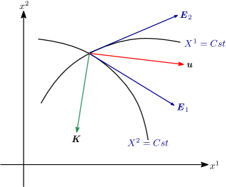
Figure 1: The material curves $X^{1}(t,x^{1},x^{2})=X^{10}$ and $X^{2}(t,x^{1},x^{2})=X^{20}$ corresponding to coordinate lines $X^{1}=X^{10}=Cst$ and $X^{2}=X^{20}=Cst$ are drawn. At any point, these curves are tangent to the vectors $\boldsymbol{E}_{2}$ and $\boldsymbol{E}_{1}$. A priori, vectors $\boldsymbol{u}$ and $\boldsymbol{K}$ are not collinear.

If theorem 8 is applied with the vorticity vector $\boldsymbol{\Omega}$, the result is trivial because $\boldsymbol{\Omega}$ and $\boldsymbol{K}$ are orthogonal. However, the result is not trivial if we use, instead of vector $\boldsymbol{\Omega}$, the column vectors ${\boldsymbol{E}}_{i},$ $i=1,2$, of the matrix $\displaystyle{\boldsymbol{F}}/{{\rm det\,\boldsymbol{F}}}$

$$\frac{\partial}{\partial t}\left(\boldsymbol{K}^{T}\boldsymbol{E}_{i}\right)+{\rm div}\left(\boldsymbol{u}\,\left(\boldsymbol{K}^{T}{\boldsymbol{E}}_{i}\right)+\left(g\,h-\frac{1}{2}\left(\frac{Dh}{Dt}\right)^{2}-\frac{|\boldsymbol{u}|^{2}}{2}\right){\boldsymbol{E}}_{i}\right)=0.$$

This equation can be interpreted as conservation laws for the covariant components of $\boldsymbol{K}$ in the basis $\boldsymbol{E}_{i}$, $i=1,2$ (see Fig 1).

6 Conclusion and discussion

We have found new conservation laws for the equations of dispersive fluids where the energy depends on the density and gradient of density (capillary fluids), or depends on the density and material time derivative of the density (fluids with internal inertia). These conservation laws keep constant generalized helicity.

We have also found new integrals representing the variation of the components of velocity $\boldsymbol{u}$ (for capillary fluids) or of vector $\boldsymbol{K}$ (for fluids with internal inertia) in a time–dependent curvilinear basis ${\boldsymbol{E}}_{i}$, $i=1,2,3$. These divergence–free basis vectors are tangent at each time to material curves along which coordinate $X^{i}$ varies and other coordinates $X^{j},\,\ j\neq i$ are fixed.

Other invariants can be found in the case when the potential $W$ depends on additional scalar transported by the fluid such as the specific entropy $\eta$. Indeed, $\eta$ satisfies the equation

$$\frac{D\eta}{Dt}=0.$$ (6.17)

The analog of Ertel’s invariant is

$$\frac{D}{Dt}\left(\frac{\partial\eta}{\partial\boldsymbol{x}}\frac{\boldsymbol{L}}{\rho}\right)=0$$

where $\boldsymbol{L}$ is either the scaled basis vectors $\boldsymbol{E}_{i}$, $i=1,2,3$  or the generalized vorticity vector. Indeed, even if the equation for the vorticity contains an extra term related to the entropy gradient, it vanishes by combining the Helmholtz equation for the generalized vorticity with the Lie derivative of covector $\displaystyle\frac{\partial\eta}{\partial\boldsymbol{x}}$ coming from (6.17) (see Appendix A for details)

$$d_{L_{1}}\left(\frac{\partial\eta}{\partial\boldsymbol{x}}\right)\equiv\frac{D}{Dt}\left(\frac{\partial\eta}{\partial\boldsymbol{x}}\right)+\frac{\partial\eta}{\partial\boldsymbol{x}}\frac{\partial\boldsymbol{u}}{\partial\boldsymbol{x}}=0.$$

In the same way, higher order conservation laws can be found as it was already done for the classical dispersionless equations (Euler equations of compressible and incompressible fluids, equations of magnetohydrodynamics, two-fluid plasma equations etc.) [7, 9, 10, 11]. However, the physical and geometrical meaning of these conservation laws still remains to be done.

Acknowledgments The authors thank Boris Haspot for helpful comments and discussions. S.G. would like to thank the Isaac Newton Institute for Mathematical Sciences, Cambridge, for support and hospitality during the programme “Dispersive hydrodynamics: mathematics, simulation and experiments, with applications in nonlinear waves” where work on this paper was undertaken. This work was supported by EPSRC grant no EP/R014604/1.

Appendix A Lie derivatives of one-form and two-form fields

In the literature, one generally uses the notation $\mathcal{L}_{\boldsymbol{v}}$ where ${\boldsymbol{v}}$ is a vector field. However, the analytical expression of the Lie derivative is different for scalars, one–forms, two–forms and so on. This is why we denote $d_{L_{1}}$ for the Lie derivative of a one–form and $d_{L_{2}}$ for the Lie derivative of a two–form [45].

We denote by $T_{\boldsymbol{x}}(\mathcal{D}_{t})$ and $T_{\boldsymbol{x}}^{\star}(\mathcal{D}_{t})$ the tangent and cotangent vector spaces at any point $\boldsymbol{x}$ of a material domain $\mathcal{D}_{t}$. A vector field $\boldsymbol{J}\in T_{\boldsymbol{x}}(\mathcal{D}_{t})$ has the inverse image $\boldsymbol{J}_{0}\in T_{\boldsymbol{X}}(\mathcal{D}_{0})$ such that

$$\boldsymbol{J}(t,\boldsymbol{x})=\boldsymbol{F}\,\boldsymbol{J}_{0}(t,\boldsymbol{X}).$$ (A.18)

Consequently, a one-form field $\boldsymbol{C}\in T_{\boldsymbol{x}}^{\star}(\mathcal{D}_{t})$ has the inverse image $\boldsymbol{C}_{0}\in T_{\boldsymbol{X}}^{\star}(\mathcal{D}_{0})$ such that

$$\boldsymbol{C}(t,\boldsymbol{x})=\boldsymbol{C}_{0}(t,\boldsymbol{X})\,\boldsymbol{F}^{-1}.$$

The Lie derivative of $\boldsymbol{C}$ is the image of  $\displaystyle{\partial\boldsymbol{C}_{0}(t,\boldsymbol{X})}/{\partial t}$  in $T_{\boldsymbol{x}}^{\star}(\mathcal{D}_{t})$ and is denoted by $d_{L_{1}}$. From the evolution equation (2.1) for $\boldsymbol{F}$, the Lie derivative $d_{L_{1}}$ of form field $\boldsymbol{C}$ is deduced from the diagram

$$\begin{array}[]{ccc}\boldsymbol{C}\in T^{\ast}_{\boldsymbol{x}}(\mathcal{D}_{t})&\begin{array}[]{c}{\boldsymbol{F}}\\ \longrightarrow\\ \\ \end{array}&\boldsymbol{C}_{0}=\boldsymbol{C}\,\boldsymbol{F}\in T^{\ast}_{\boldsymbol{X}}(\mathcal{D}_{o})\\ \begin{array}[]{c}\displaystyle d_{L_{1}}\,\Big{\downarrow}\\ \end{array}&&\begin{array}[]{c}\displaystyle\Big{\downarrow}\,\displaystyle\frac{D}{Dt}\\ \end{array}\\ \begin{array}[]{c}\\ \displaystyle\frac{D\boldsymbol{C}}{Dt}+\boldsymbol{C}\,\displaystyle\frac{\partial\boldsymbol{u}}{\partial\boldsymbol{x}}\in T^{\ast}_{\boldsymbol{x}}(\mathcal{D}_{t})\end{array}&\begin{array}[]{c}{\boldsymbol{F}}^{-1}\\ \longleftarrow\\ \end{array}&\begin{array}[]{c}\\ \ \ \ \displaystyle\frac{D\boldsymbol{C}}{Dt}\boldsymbol{F}+\boldsymbol{C}\,\displaystyle\frac{\partial\boldsymbol{u}}{\partial\boldsymbol{x}}\boldsymbol{F}\in T^{\ast}_{\boldsymbol{X}}(\mathcal{D}_{o})\end{array}\end{array}$$

Consequently, the Lie derivative of $\boldsymbol{C}$ is

$$d_{L_{1}}\boldsymbol{C}={\frac{{D\boldsymbol{C}}}{Dt}}+\boldsymbol{C}\,\frac{\partial\boldsymbol{u}}{\partial\boldsymbol{x}}\equiv\frac{\partial\boldsymbol{C}}{\partial t}+\boldsymbol{u}^{T}\left(\frac{\partial\boldsymbol{C}^{T}}{\partial\boldsymbol{x}}\right)^{T}+\boldsymbol{C}\,\frac{\partial\boldsymbol{u}}{\partial\boldsymbol{x}}.$$

A two-form field $\boldsymbol{\omega}\in T_{\boldsymbol{x}}^{2\star}(\mathcal{D}_{t})$ has the inverse image $\boldsymbol{\omega}_{0}\in T_{\boldsymbol{X}}^{2\star}(\mathcal{D}_{0})$. There exists an isomorphism $\boldsymbol{\omega}(t,\boldsymbol{x})\in T_{\boldsymbol{x}}^{2\star}(\mathcal{D}_{t})\longrightarrow\boldsymbol{w}(t,\boldsymbol{x})\in T_{\boldsymbol{x}}(\mathcal{D}_{t})$ defined as

$$\forall\ \boldsymbol{J}_{1}\ \text{and}\ \boldsymbol{J}_{2}\in T_{\boldsymbol{x}}(\mathcal{D}_{t}),\quad\boldsymbol{\omega}\,(\boldsymbol{J}_{1},\boldsymbol{J}_{2})=\text{det}\,(\boldsymbol{w},\boldsymbol{J}_{1},\boldsymbol{J}_{2}).$$

We can define a vector field $\boldsymbol{w}_{0}$ such that:

$$\text{det}\,\left(\boldsymbol{w},\boldsymbol{J}_{1},\boldsymbol{J}_{2}\right)=\text{det}\,(\boldsymbol{w_{0}},\boldsymbol{J}_{10},\boldsymbol{J}_{20})$$

where $\boldsymbol{J}_{10}$ and $\boldsymbol{J}_{20}$ are the inverse image in $T_{\boldsymbol{X}}(\mathcal{D}_{0})$ of $\boldsymbol{J}_{1}$ and $\boldsymbol{J}_{2}$ which verify (A.18). Similarly to the proof of lemma 1, we obtain

$$\boldsymbol{w}\,(t,\boldsymbol{x})=\frac{\boldsymbol{F}}{\text{det}\,\boldsymbol{F}}\,\boldsymbol{w}_{0}\,(t,\boldsymbol{X})\qquad{\rm or}\qquad\boldsymbol{w}_{0}\,(t,\boldsymbol{X})=({\text{det}\,\boldsymbol{F}})\,\boldsymbol{F}^{-1}\boldsymbol{w}\,(t,\boldsymbol{x}).$$

The Lie derivative $d_{L_{2}}$ of $\boldsymbol{\omega}(t,\boldsymbol{x})$ is isomorphic to the image of $\displaystyle\frac{\partial\boldsymbol{w}_{0}(t,\boldsymbol{X})}{\partial t}$  and we deduce from (2.1)

$$\text{det}\,\left(d_{L_{2}}{\boldsymbol{w},\boldsymbol{J}_{1},\boldsymbol{J}_{2}}\right)=\text{det}\,\left(\frac{D\boldsymbol{w}}{Dt}+\boldsymbol{w}\,\text{div}\,\boldsymbol{u}-\frac{\partial\boldsymbol{u}}{\partial\boldsymbol{x}}\,\boldsymbol{w},\boldsymbol{J}_{1},\boldsymbol{J}_{2}\right),$$

or

$$d_{L_{2}}{\boldsymbol{w}}=\frac{D\boldsymbol{w}}{Dt}+\boldsymbol{w}\,\text{div}\,\boldsymbol{u}-\frac{\partial\boldsymbol{u}}{\partial\boldsymbol{x}}\,\boldsymbol{w}.$$

Let us note that $d_{L_{1}}\boldsymbol{C}$ and $d_{L_{2}}\boldsymbol{w}$ are zero if and only if $\boldsymbol{C}_{0}$ and $\boldsymbol{w}_{0}$ do not depend on time $t$ (they depend only on $\boldsymbol{X}$). A typical example of the two-form field is the vorticity vector. Another important example is the cross product of two one-forms $\ \displaystyle\frac{\partial\alpha}{\partial\boldsymbol{x}}\times\frac{\partial\beta}{\partial\boldsymbol{x}}$, where $\alpha$ and $\beta$ are two scalar fields [45].

References

[1] Moreau J J 1961 Constantes d’un îlot tourbillonnaire en fluide parfait barotrope C. R. Acad. Sci. Paris252 2810–2812
[2] Moffatt H K 1969 The degree of knottedness of tangled vortex lines J. Fluid Mech.35 117–129
[3] Gouin H 1976 Noether theorem in fluid Mechanics Mech. Res. Comm.3 151–155
[5] Salmon R 1998 Lectures on Geophysical Fluid Mechanics Oxford University Press
[6] K Araki 2015 Helicity-based particle-relabeling operator and normal mode expansion of the dissipationless incompressible Hall magnetohydrodynamics Phys. Rev. E92 063106
[7] Tur A V and Yanovsky V V 1993 Invariants in dissipationless hydrodynamic media J. Fluid Mech.248 67–106
[8] Arnold V I and Khesin B A 1998 Topological Methods in Hydrodynamics Applied Mathematical Sciences Vol. 125 Springer
[9] Cotter C J and Holm D D 2013 On Noether’s Theorem for the Euler–Poincaré
Equation on the Diffeomorphism Group with Advected Quantities Found. Comput. Math.13 457–477
[10] Webb G M, Dasgupta B, McKenzie J F, Hu Q and Zank G P 2014 Local and nonlocal advected invariants and helicities in magnetohydrodynamics and gas dynamics: II. Noether’s theorems and Casimirs
J. Phys. A Mathematical and Theoretical47 095502
[11] Cheviakov A F and Oberlack M 2014 Generalized Ertel’s theorem and infnite
hierarchies of conserved quantities for
three-dimensional time-dependent Euler and Navier-Stokes equations J. Fluid Mech.760 368–386
[12] Moffatt H K 2018 Helicity C. R. Mécanique Acad. Sci. Paris346 165–169
[13] Irvine W T M 2018 Moreau’s hydrodynamic helicity and the life of vortex knots and links C. R. Mécanique Acad. Sci. Paris346 170–174
[14] Serre D 2018 Helicity and other conservation laws in perfect fluid motion C. R. Mécanique Acad. Sci. Paris346 175–-183
[15] Casal P 1963 Capillarité interne en mécanique des milieux
continus C.R. Acad. Sci. Paris256 3820–3823
[16] Eglit M E 1965 A generalization of the model of compressible fluid J. Appl. Math. Mech.29, 351–354
[18] Casal P and Gouin H 1985 Relation entre l’équation de
l’énergie et l’équation du mouvement en théorie de Korteweg de
la capillarité C. R. Acad. Sci. Paris300 II
231–234
[19] Gavrilyuk S and Shugrin S 1996 Media with equations of state that depend on derivatives J. Appl. Mech. Techn. Phys.37 179–189.
[20] Benzoni-Gavage S, Danchin R, Descombes S and Jamet D 2005 On Korteweg Models for Fluids Exhibiting Phase Changes Interfaces Free Bound.7 371–414
[21] Garajeu M, Gouin H and Saccomandi G 2013 Scaling Navier-Stokes equation in nanotubes Physics of Fluids25 082003
[22] Gouin H and Saccomandi G 2016 Travelling waves of density for a fourth-gradient model of fluids Continuum Mechanics and Thermodynamics28 1511–1523
[23] Audiard C and Haspot B 2018 From Gross–Pitaevskii equation to Euler–Korteweg system, existence of global strong solutions with small irrotational initial data Annali di Matematica Pura ed Applicata197 721–760
[24] Bresch D, Gisclon M and Lacroix-Violet I 2019 On Navier–Stokes–Korteweg and Euler–Korteweg systems: Application to quantum fluids models Arch.
Ration. Mech. Anal.233 975–1025
[25] Gavrilyuk S and Gouin H 2020 Rankine–Hugoniot conditions for fluids whose energy
depends on space and time derivatives of density Wave Motion98 102620
[26] Iordansky S V 1960 About equations of motion of fluid containing the gas bubbles J. Appl. Mech. Techn. Physics3 102-110
[27] Kogarko B S 1961 On a model of a cavitating liquid Dokl. Akad. Nauk SSSR137 1331–1333
[28] van Wijngaarden L 1968 On the equations of motion for mixtures of liquid and gas bubbles J. Fluid Mech.33 465–474
[29] Gavrilyuk S L and Teshukov V M 2001 Generalized vorticity for bubbly liquid and dispersive shallow water equations Continuum Mechanics and Thermodynamics13 365–382
[30] Gavrilyuk S 2011 Multiphase Flow Modeling via Hamilton’s principle In Variational Models and Methods in Solid and Fluid Mechanics CISM Courses and Lectures Vol. 535 pp. 163–210 (Eds. F dell’Isola and S Gavrilyuk) Springer Berlin
[31] Serre F 1953 Contribution à l’étude des écoulements permanents et variables dans les canaux
La Houille blanche8 830–-872
[32] Green A E and Naghdi P M 1976 A derivation of equations for wave propagation in water of variable depth J. Fluid. Mechanics78 237–246
[33] Lannes D 2013 The Water Waves Problems Mathematical Surveys and Monographs188 AMS Providence RI
[34] Gavrilyuk L and Gouin H 1999 A new form of governing equations of fluids arising from Hamilton’s principle International Journal of Engineering Science37 1495–1520
[35] Gurtin M E, Fried E and Anand L 2007 The Mechanics and Thermodynamics of Continua, Cambridge University Press
[36] Gavrilyuk S, Gouin H and Perepechko Yu 1998 Hyperbolic models of homogeneous two–fluid mixtures Meccanica33 161–175
[37] Duchêne V and Israwi S 2018 Well–posedness of the Green–Naghdi and Boussinesq–Peregrine systems Annales Math Blaise Pascal25 21–74
[38] Le Métayer O, Gavrilyuk S and Hank S 2010 A numerical scheme for the Green–Naghdi model J Comp Physics229 2034–2045
[39] Lannes D and Marche F 2016 Nonlinear wave-current interactions in shallow water Studies in Applied Mathematics136 382–423
[40] Favrie N and Gavrilyuk S 2017 A rapid numerical method for solving Serre-
Green-Naghdi equations describing long free surface gravity waves Non-
linearity30 2718–-2736
[41] Duchêne V and Klein C 2022 Numerical study of the Serre–Green–Naghdi equations and a fully dispersive counterpart Discrete and Continuum Dynamical Systems B27 5905–5933
[42] Camassa R, Holm D D and Levermore C D 1997 Long-time shallow–water equations with a varying bottom J. Fluid Mech.349 173–189
[43] Gavrilyuk S, Kalisch H and Khorsand Z 2015 A kinematic conservation law in free surface flow Nonlinearity28 1805–1821
[44] Matsuno Y 2016 Hamiltonian structure for two-dimensional extended Green-Naghdi equations Proc Royal Soc Math Phys Eng Sci 472 2190
[45] Gouin H 2023 Remarks on the Lie derivative in fluid mechanics Int. J. Non-Linear Mechanics150 104347