Efficacy of the Sterile Insect Technique in the presence of inaccessible areas: A study using two-patch models
Abstract
The Sterile Insect Technique (SIT) is one of the sustainable strategies for the control of disease vectors, which consists of releasing sterilized males that will mate with the wild females, resulting in a reduction and, eventually a local elimination, of the wild population. The implementation of the SIT in the field can become problematic when there are inaccessible areas where the release of sterile insects cannot be carried out directly, and the migration of wild insects from these areas to the treated zone may influence the efficacy of this technique. However, we can also take advantage of the movement of sterile individuals to control the wild population in these unreachable places. In this paper, we derive a two-patch model for Aedes mosquitoes where we consider the discrete diffusion between the treated area and the inaccessible zone. We investigate two different release strategies (constant and impulsive periodic releases), and by using the monotonicity of the model, we show that if the number of released sterile males exceeds some threshold, the technique succeeds in driving the whole population in both areas to extinction. This threshold depends on not only the biological parameters of the population but also the diffusion between the two patches.
Pierre-Alexandre Bliman111MAMBA, Inria Paris; LJLL, Sorbonne University, CNRS, 5 Place Jussieu, 75005 Paris, France (email : pierre-alexandre.bliman@inria.fr)., Nga Nguyen222LAGA, CNRS UMR 7539, Institut Galilée, Université Sorbonne Paris Nord, 99 avenue Jean-Baptiste Clément, 93430 Villetaneuse; MAMBA, Inria Paris, Laboratoire Jacques Louis-Lions, Sorbonne Université, 5 place Jussieu, 75005 Paris, France (email : thiquynhnga.nguyen@math.univ-paris13.fr)., Nicolas Vauchelet333LAGA, CNRS UMR 7539, Institut Galilée, Université Sorbonne Paris Nord, 99 avenue Jean-Baptiste Clément, 93430 Villetaneuse, France (email : vauchelet@math.univ-paris13.fr).
Keywords: sterile insect technique, metapopulation model, monotone dynamical systems
1 Introduction
Mosquitoes of genus Aedes aegypti and Aedes albopictus play a crucial role in transmitting various arboviruses to humans including dengue, chikungunya, and Zika virus. Unfortunately, there are no specific vaccines or drugs available for these diseases. Consequently, the primary prevention lies in controlling the mosquito population [37]. However, traditional insecticide-based methods have limitations, prompting the need for innovative and sustainable strategies [2], [10]. Biological controls involve releasing large numbers of mosquitoes that are either sterile or incapable of transmitting diseases, which recently gained much attention. The Sterile Insect Technique is among these sustainable alternative methods which consist of the release of sterilized male mosquitoes that will mate with wild females [21], [19]. These wild females, unable to lay viable eggs, will gradually drive the wild population to decline. The efficacy of SIT relies on a comprehensive understanding of the vector behavior, as well as accurate modeling of its dispersal, to optimize the release strategies.
Spatial heterogeneity in mosquito populations and mosquito-borne diseases occurs due to differences in the quality and quantity of their habitats, as well as variations in host density, temperature, and rainfall [15], [34], [31]. Especially, the number and accessibility of sites where mosquitoes lay their eggs play a significant role in determining the size of adult mosquito populations by increasing the carrying capacity of the environment [1]. Developing models that capture mosquito behavior in response to environmental heterogeneity is crucial for designing effective control strategies, especially in the face of rapid global land-use changes. Models using monotone dynamical systems were introduced (see e.g. [7], [18], [35]) and applied efficiently (see e.g. [11], [8], [12]) to study the SIT. Not many mosquito modeling studies have incorporated migration or dispersal effects due to insufficient information on individual movement in the field as well as the complex analysis of models. Most of them used the diffusion approach, which considers space as a continuous variable. They were first developed in one-dimensional space using scalar reaction-diffusion equations [30], [25], then extended to sex-structured compartmental systems to consider the different behaviors of aquatic phases, wild females, males, and sterile males (see e.g. [4], [6], [24]) and in higher dimension (see e.g. [17], [5]). However, it remains challenging to explicitly incorporate the factors that affect the movement of sterile males. For instance, when resources are concentrated in patches or distinct locations, a metapopulation approach in which we treat space as a discrete set of patches and describe how the population on each patch varies with time is more suitable for modeling mosquito dispersal [9], [28], [29].
The application of the SIT in the field encounters a difficulty of the limitation in space when there are some inaccessible areas where people can not release sterile insects directly. For example, mosquitoes of the genus Aedes polynesiensis primarily exploit land crab burrows for oviposition in certain French Polynesian atolls [13], [22], [23], [20]. The larvae in the crab burrows emerge into adult mosquitoes that can fly out to search for food and human blood for fertility. However, one standout advantage of the SIT is that it relies on the natural ability of the male mosquitoes to move, locate, and mate with females. This behavior will take place in those areas that cannot be reached with conventional control techniques (i.e. insecticides). Therefore, we are interested in the mosquito population dynamics in the presence of such reservoirs and the elimination of the whole population while considering that the released sterile males can fly into unreachable sites. The patchy models with discrete diffusion mentioned above are a useful approach to describe the mosquito dynamic taking into account the inaccessibility to the burrows. We develop a two-patch model and in each patch, we consider a monotone dynamical system inspired by the models in [35] where the population is divided into different compartments characterizing the aquatic phase, wild females, wild males, and sterile males. Except for the aquatic phase, individuals in other states move between patches at specific rates. The SIT is only carried out in the first patch and only affects the second one through these natural movements. Two-patch models were used to study the same problem in [38], where they considered a simple scalar equation to describe the population dynamics in each patch. Our model provides a better understanding of how the dynamics of each stage influence the result of the control method. However, the complexity of our system does not allow us to obtain the full analysis of the model like what has been done in [38].
In the present work, we are interested in how to guarantee the successful elimination of the SIT in both areas and how the diffusion rates as well as other biological parameters influence the efficacy. To tackle this problem, we focus on studying the global stability of the extinction equilibrium in our system. Results of global asymptotic behavior for the single-species model depending on the discrete diffusion were provided in the literature[3], [36], [27]. Lyapunov’s second method was used in [26] to investigate the multi-species system with discrete diffusion. Many works have been done to design robust strategies for releasing sterile males to drive a population to elimination [11], [12]. We extend these control strategies to our two-patch system and prove the sufficient conditions for both constant continuous and periodic impulsive releases to drive the whole system to extinction. We obtain that when the number of released sterile males exceeds some threshold, the populations in both the treated and the inaccessible zone reach elimination. We also show in the present work how the diffusion rates between two areas and other biological parameters influence these conditions. These results may help estimate the possibility and the surplus of sterile mosquitoes necessary to complete elimination in the presence of hidden, inaccessible, reservoirs.
The organization of the paper is as follows. In section 2, we present the formulation of the two-patch model and prove the monotonicity of the systems and some other preliminary results that be applied in our proofs. Section 3 is devoted to the study of the system without sterile insects. In Theorem 3.1, we provide conditions for the persistence and extinction of the wild population on each patch. In section 4, we study the dynamics of mosquito population in the presence of the SIT with two release strategies: constant and impulsive releases. Theorem 4.2 presents sufficient conditions on the average number of sterile males released per time unit to drive the population to elimination. We provide the principle of the method used to treat the system in 4.1 and then apply this principle to prove Theorem 4.2. Section 5 is focused on the dependence of the critical number of sterile males on parameters. The results in 5.1.1 show that when the diffusion rates are large, the dynamics of the whole system are the same as in the case when there is no separation between the two sub-populations. Then, Theorem 5.3 shows that the critical number of released sterile males depends monotonically on the biological parameters. Finally, some numerical illustrations are provided in Section 6.
2 Model
In this section, we present the formulation of the model used to study the population dynamics in 2.1. Then, in 2.2, we provide some preliminary results that will be used later in the present work.
2.1 Formulation of the model
Consider two patches and denote , and respectively the density of aquatic phase (eggs, larvae, pupae), fertile females, males, and sterile males on the patch depending on time . We consider a two-patch model coupled by the diffusion terms as follows where the dynamic in each patch is inspired by the model in [35]
| (1a) | ||||
| (1b) | ||||
| (1c) | ||||
| (1d) | ||||
| (1e) | ||||
| (1f) | ||||
| (1g) | ||||
| (1h) | ||||
The interpretation of the parameters used in the model, with , is as below
-
•
is the number per time unit of sterile mosquitoes that are released at time on the first patch;
-
•
the fraction corresponds to the probability that a female mates with a fertile male;
-
•
is the birth rate; , , and denote the death rates for the mosquitoes in the aquatic phase, for adult males, and for adult females, respectively;
-
•
is an environmental capacity for the aquatic phase on patch th, accounting also for the intraspecific competition;
-
•
is the rate of emergence;
-
•
is the probability that a female emerges, then is the probability that a male emerges.
-
•
is the moving rate of female mosquitoes from patch th to patch th; the fertile males and sterile males move slower but with proportional rates respectively , where typically in practice.
We recall the basic offspring number of the sub-population in one patch as introduced in [35]
| (2) |
The persistence and extinction of the population in the patch depend strongly on the value of this number. In Section, 3, we will show that is also the basic offspring number of the whole two-patch system.
2.2 Preliminary results
First, we provide some definitions and denotations of the order used in the present work.
Definition 2.1.
A matrix is called non-negative, denote , if all of its entries are non-negative.
It is called positive, denote , if it is non-negative and there is at least one positive entry.
It is called strictly positive, denote , if all of its entries are strictly positive.
In the present work, we also use the above definition of order for vectors in . Next, we present a property of a Metzler matrix that will be used in this paper.
Lemma 2.1.
Assume that a square matrix is Metzler and irreducible, then is strictly positive.
Proof.
Since is Metzler, then there exists a constant large enough such that is a non-negative matrix with a positive element on the main diagonal. Moreover, is irreducible so is also irreducible. Thus, is primitive, that is, there exists an integer such that . Hence, we have , and since commutes with all matrices, one has . ∎
We present in this section the so-called Kamke [16] or Chaplygin [14] lemma for a cooperative system (Lemma 2.2). Then, we apply this lemma to show the monotonicity of system (1) in Lemma 2.3.
Lemma 2.2.
For any , consider a smooth function , and a vector function satisfying a differential equation
Moreover, we assume that the above system is cooperative, that is,
| (3) |
If a vector function satisfies a differential inequality then, for initial data , we have for all .
To apply this Lemma to system (1), we first define the following order in as follows
Definition 2.2.
For any vectors , we define an order such that if and only if
Moreover, we write if and .
The monotonicity of system (1) is shown in the following result
Lemma 2.3.
Proof.
By changing the variable to , we can write system (1) as
This system is cooperative since in of , we have
Similarly for with , so is cooperative.
For any vector function such that , by the same variable change, one has . The initial data implies that . Therefore, by applying Lemma 2.2, one has for any which is equivalent to . ∎
In order to define the solution of (1), we make some assumptions for the release function
Assumption 2.1.
Assume that function satisfies
| (4) |
where , for almost every , and is a sum of Dirac masses with positive weights. Assume moreover that there exists a time such that the average value of over any -time interval is finite, that is,
| (5) |
Assumption 5 is natural since in practice, the total amount of the sterile males released in a finite time interval is finite. The term corresponds to impulsive releases.
The next result shows that any trajectory of system (1) resulting from any non-negative initial data is bounded.
Lemma 2.4.
Remark 2.1.
In the case , one can let tend to zero and obtain that and . The condition of that we made in Assumption 5 is weaker than the assumption since we also include impulsive releases, represented by the Dirac masses.
Proof of Lemma 2.4.
For , we have and assume that there exists a value such that
then but from (1a) and (1e), one has (contradictory). Then we deduce that for any .
From equations (1b) and (1f), since for , one has
Since are bounded then we deduce that
for any . For , one has , thus for any . Let goes to infinity we get . One obtains similarly the inequalities for .
For and , by denoting , then from equations (1d) and (1h), one has
For any integer , by integrating both sides of this equality in with defined in Assumption 5, one gets
Since for any and by Assumption 5, we deduce that
with defined in (5). Using the iteration with respect to , we deduce that
Now for any time , there exists an integer such that . Then, we obtain that
since . The inequality of follows. ∎
3 Mosquito dynamics without sterile males
First, we describe the dynamics of wild mosquitoes in the two areas by considering the following system which is re-obtained from system (1) in the absence of sterile males
| (6a) | ||||
| (6b) | ||||
| (6c) | ||||
| (6d) | ||||
| (6e) | ||||
| (6f) | ||||
It is clear that the subset of the positive cone of is positively invariant over time. The following result shows the nature of the equilibrium points of system (6).
Theorem 3.1.
Theorem 3.1 shows that the constant defined in (2) is the basic offspring number of the whole two-patch system (1). When , the populations in both areas remain persistent for any diffusion rates as time evolves. In the rest of the paper, we only consider the case .
To prove this theorem, we first consider the sub-system of . From equations (6b) and (6e), the positive equilibrium satisfies
then
| (7) |
On the other hand, from equation (6a) and (6d), we also have
| (8) |
From (7) and (8), we deduce that
| (9) |
| (10) |
The following lemma provides information for these functions.
Lemma 3.2.
For , function is defined and convex on .
If , then has no positive root and it is increasing on .
Otherwise, it has a unique positive root
| (11) |
Moreover, on , and increasing on .
Proof of Lemma 11.
We recall function . One has if and only if
We deduce that at and as in (11) , and if and only if . Moreover, on , and is increasing on . It is defined and convex on since
for any . We also have , . ∎

Proof of Theorem 3.1.
Existence and uniqueness of the positive equilibrium. System (6) has a positive equilibrium iff system (9)-(10) has a solution in .
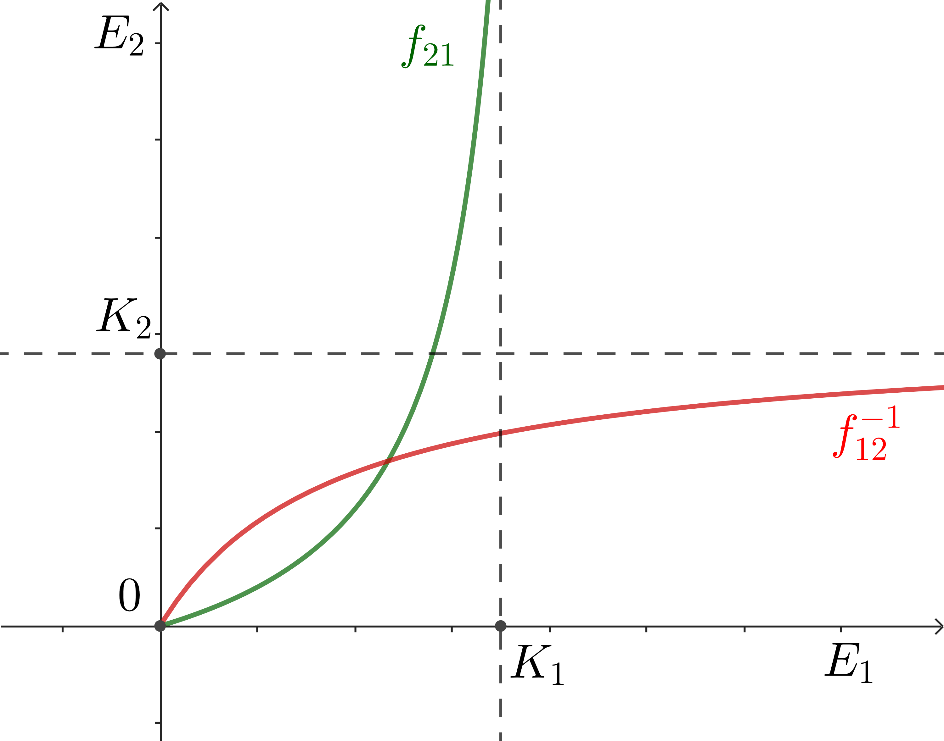
First, we study the case where , then according to Lemma 11, we have is positive and increasing, so this function is invertible (see Figure 1). We denote the restriction of the invert function of on , then
Thus, is a positive root of function . For any , one has
then
since is convex on . Hence, is convex on . Moreover, we have , and . Therefore, this function has a unique positive root if and only if the derivative at zero is negative. We have
Then, if and only if .
Now, without loss of generality, we assume that , then . If , again according to Lemma 11, function has a unique positive root and is invertible on (see Figure 1). We denote again the restriction of the invert function of on , then we also have convex on , and , . We can deduce that has a unique positive root on .
Instability of the zero equilibrium. At the origin of , the Jacobian matrix of system (6) is
with the characteristic polynomial
Since , we have . Thus, we can deduce that the factor has one positive root . Hence, the Jacobian at zero has at least one positive eigenvalue so the zero equilibrium is unstable.
Stability of the positive equilibrium. First, we can see that the system (6a)-(6b), (6d)-(6e) of does not depend on , and it is cooperative and irreducible. By applying Theorem 1.1 in Chapter 4 of [33], one deduces that this system is strongly monotone. When , this system admits exactly two equilibria: , and . But the zero equilibrium is unstable, so by Theorem 2.2 in Chapter 2 of [33], if the initial data satisfies that , the solution converges to when .
Now if the initial data satisfies that , then there exists a constant large enough such that . Since , one has
and the right-hand side of system (6a)-(6b), (6d)-(6e) at is non positive. Thus, the trajectory resulting from the initial data is non-increasing, and therefore converges to . By applying the Lemma 2.2 to system (6a)-(6b), (6d)-(6e), we deduce that the trajectory resulting from the initial data lies between and the trajectories resulting from . Hence, it also converges to when time goes to infinity.
Moreover, since the trajectories issued from the initial data above and below all converge to the same limit, then by the comparison principle, we deduce that the trajectory resulting from any positive initial data with values between these initial values converges to this equilibrium.
Secondly, if we denote matrix , this matrix is Hurwitz. Functions satisfy . Thus, for any ,
| (12) |
Moreover, the equilibrium satisfies
| (13) |
Hence, from (13) and (12), we deduce that
| (14) |
Moreover, when , we have that converges to and since is Hurwitz. Thus, for any , there exists a time large enough such that for any ,
| (15) |
and .
Since matrix is Metzler and irreducible, then by applying Lemma 2.1, one has that is strictly positive for any . Moreover, one has in , then for any ,
then
with some positive constant not depending on . Using the second inequality in (15), one has
Proving similarly for the other inequality, we can deduce that
with some positive constant not depending on . Hence, from (14), we deduce that for any ,
Therefore, converges to when tends to . ∎
In the following section, by considering the releases of sterile males, we look for a condition of release functions such that the positive equilibrium disappears.
4 Elimination with releases of sterile males
In this section, we consider in system (1) the number of sterile males released per time unit and our goal is to adjust its values such that the wild population reaches elimination. We consider two release strategies as follows
Constant release: Let the release function . As time goes to infinity, the density of sterile males converges to that is the solution of system
| (16) |
By denoting
| (17) |
we have , and and .
Impulsive periodic releases: Consider the release function
| (18) |
with period and is the average number of sterile males released per time unit during the time interval for . We choose in this work constant and drop consequently the sub-index . The release function in (18) means that we release a total amount of mosquitoes at the beginning of each time period ().
Denote vector , then with , the density of sterile males satisfies the following system
| (19a) | ||||
| (19b) | ||||
with matrix , and denote the right and left limits of at time and by convention, we set . The densities of the sterile males evolve according to (19a) on the union of open intervals while is submitted to jump at each point as in (19b). For such a release schedule, the solution of system (19) satisfies
Since matrix is Hurwitz, when , we have that converges to the periodic solution that satisfies that, for
| (20) |
The following lemma shows that the periodic solution is strictly positive at any time .
Lemma 4.1.
There exists positive constant which depends on and period such that for any , one has .
Proof.
We have matrix is Metzler and irreducible, then by applying Lemma 2.1, we deduce that .
On the other hand, matrix is Hurwitz so for any . Moreover, we have is also strictly positive for any , thus there exist positive constants depending on and such that
The result of Lemma 4.1 follows. ∎
Remark 4.1.
The parameters defined in (17) and play a similar role to each other: they define a relationship between an average release rate per time unit and a (minimum) level of the sterile mosquito density.
We provide in the following result a condition on for the wild population to reach elimination.
Theorem 4.2.
Consider system (1) with the release function . Then
- •
-
•
In the periodic release case, for defined in (19), There exists a positive constant satisfying
with defined in Lemma 4.1, defined in Lemma 2.4 such that if , then for any non-negative initial data, the solution of the initial value problem of system (1) converges to the unique steady state
as time .
This result shows that with a sufficiently large number of sterile males released in the first zone, we can succeed in driving the wild population in both areas to elimination. In the following, we describe the principle idea to prove this result.
4.1 Principle of the method
To provide conditions for the release to stabilize the zero equilibrium, our strategy is as follows:
Step 1: We consider , for , in system (1) to be smaller than some level, then we study the system with the fractions replaced by some constant.
Step 2: We show how to realize, through an adequate choice of , the above behavior of .
4.1.1 Step 1: Setting the sterile population level directly
Theorem 3.1 shows us that when the basic offspring number is smaller than 1, the zero equilibrium is globally asymptotically stable. For the controlled system, the basic offspring numbers are smaller than . It suggests that for stabilizing the origin of system (1), it is sufficient to ensure .
Proposition 4.3.
Proof.
Assume that we can set to be large enough such that (21) holds, and we consider the following system
| (22a) | ||||
| (22b) | ||||
| (22c) | ||||
| (22d) | ||||
| (22e) | ||||
| (22f) | ||||
Denote solution of system (22). Since system (22) is cooperative and the inequality (21) holds, one obtains that is a super-solution of the system (1a)-(1c), (1e)-(1g), and by applying Lemma 2.2, we have .
Denote a positive equilibrium of system (22) if exists. Similar to the previous section, we have
| (23) |
| (24) |
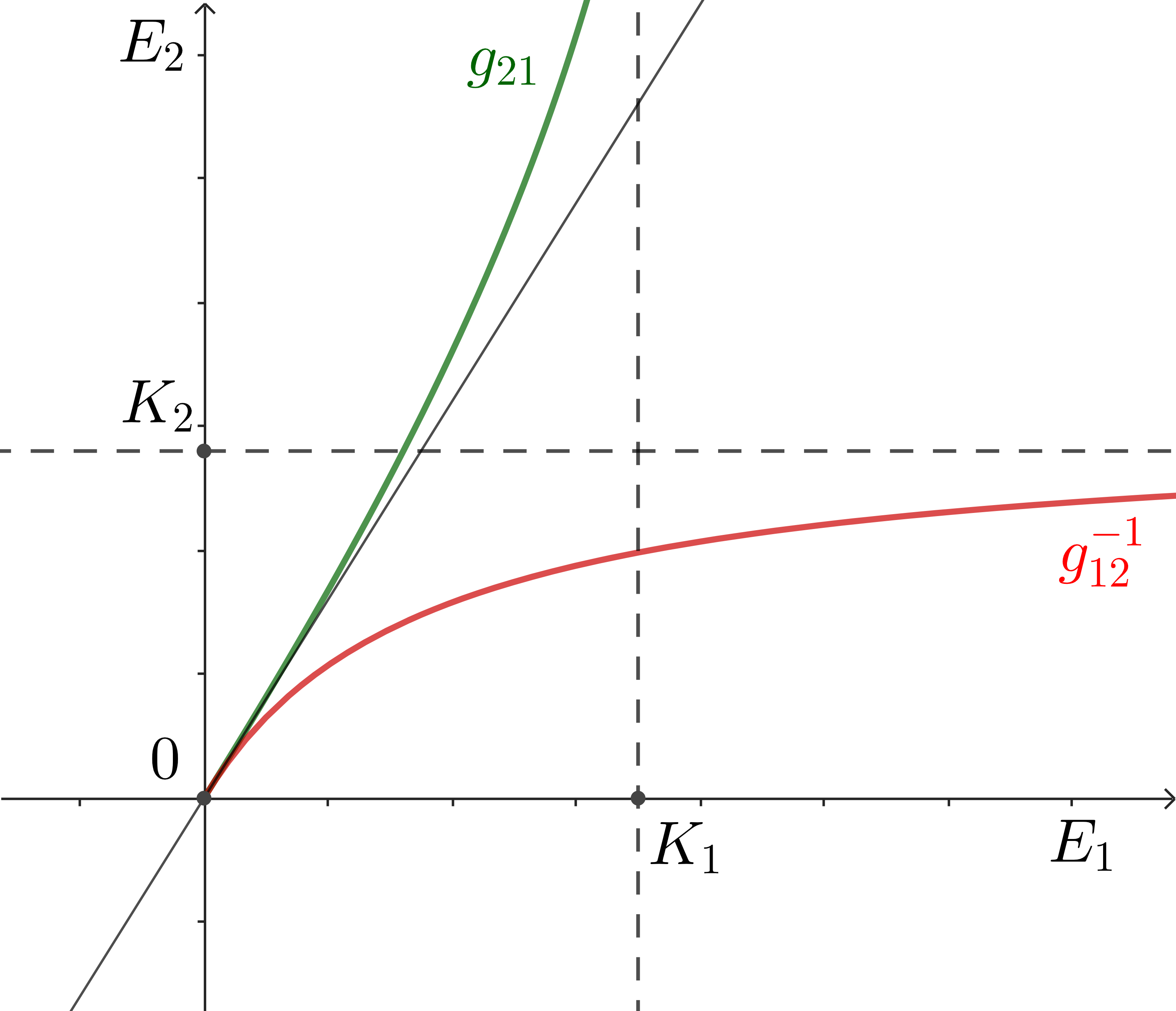
The analysis of is analogous to in Lemma 11. It is easy to check that is increasing on , so it is invertible. Then, satisfies . Function is convex and is concave in , and
We obtain that (see Figure 2), so zero is the unique equilibrium of system (22). By applying Theorem 3.1 in Chapter 2 of [33], we deduce that when , the solution converges to the equilibrium zero. Since for all , we deduce that the also converges to zero when large.
∎
4.1.2 Step 2: Shaping the release function
4.2 Proof of Theorem 4.2
Proof of Theorem 4.2.
Constant release: For , let us recall , and it is a Hurwitz matrix. And we have
Thus, when , we can deduce that converges to for any initial data since when . Hence, for any , there exists a value such that for any , ,
If we take such that with defined in Lemma 2.4, then condition (21) holds. By applying Proposition 4.3, we deduce that for , if , system (1) has as a unique equilibrium point, and every trajectory converges to this equilibrium when . The dynamics of system (1) depend continuously and monotonically on , then we deduce that there exists a positive critical value such that for any , and for any non-negative initial data, solution converges to when .
Impulsive periodic releases: Consider defined in (19), denote a solution of (1a)-(1c), (1e)-(1g) with defined in (20). From Lemma 4.1, one has for all . Therefore, if we take such that , then condition (21) holds. By applying Proposition 4.3, we deduce that converges to zero as grows. Since converges to as , we have appoaches and thus converges to as time goes to infinity.
5 Parameter dependence of the critical values of the release rate
In this section, we consider the constant release case and examine how the critical value depends on the parameters of system (1). In this model, the elimination of the population depends not only on the diffusion rate between the inaccessible area and the treated area, but also on the biological intrinsic values like the birth/death rates, and the carrying capacity.
5.1 Diffusion rates
In this part, we want to compare the critical values of corresponding to different values of . We show that when the diffusion rates are large enough, the critical number of sterile males released is the same as in the case when there is no separation between the two sub-populations.
5.1.1 The case large
First, we present a result of uniform convergence of system (1) when go to and is proportional to .
Proposition 5.1.
For , consider the diffusion rates with . Denote the solution of system (1) with the initial date satisfying that
and
| (25) |
Then, when , the sequence converges uniformly to a limit on . Moreover, we have
| (26) |
If we denote , then solves the following system
| (27a) | ||||
| (27b) | ||||
| (27c) | ||||
| (27d) | ||||
| (27e) | ||||
with the corresponding initial data .
It is straightforward to see that the previous result implies that the functions fulfill the following identities:
Proof of Proposition 5.1.
To prove this result, we first apply the Arzela-Ascoli theorem for the sequence of smooth solution on a close interval with any . Then, we extend the convergence at infinity.
Uniform convergence on : First, we check the uniform boundedness of this sequence. For , from Lemma 2.4, one has for all and . Again by this Lemma, for any , one has
where does not depend on since the initial data converge as goes to zero. Similarly, we can apply Lemma 2.4 to show that there are positive constants not depending on such that for any , one has .
Next, we prove that the sequence of derivative is also uniformly bounded. For any ,
We show that is uniformly bounded on . Indeed, we have for all and ,
where is uniformly bounded since we already proved that is uniformly bounded. Then, for any , we have for any and some constant . By the Duhamel formula, we obtain
So for all , one has
For any and , one has . And due to the Assumption (25) for the initial data, the right-hand side is uniformly bounded with respect to . Hence, we deduce that is uniformly bounded on . We obtain analogously the uniform boundedness of and . Due to the positivity of system (1), one has for all and .
Since the sequence of derivatives is uniformly bounded on , we deduce the equicontinuity of the sequence . Hence, by the Arzela-Ascoli theorem, this sequence has a uniformly convergent subsequence. We denote its limit . If we multiply system (1) with and let it go to zero, we obtain the equalities (26) and system (27).
With the initial data satisfying the assumptions in Proposition 5.1, the solution of system (27) on is unique. Since all the subsequence of converge to the same limit, we deduce that the whole sequence converges uniformly to this limit on .
Extension to : For all , we prove that for all , there exists such that for all , we have .
Indeed, the solution of both (1) and (27) converges to a constant as time goes to infinity, then there exists a time large enough and such that for any and all , one has
Moreover, we have that the sequence converges uniformly to in the closed interval . Thus, there exists a positive value such that for all ,
Hence, we have and we deduce that
It is clear that for , one has . So we obtain the convergence on . ∎
In the next result, we study the limit system (27).
Theorem 5.2.
Consider system (27) with the release function given by
-
(i)
constant release .
Then there exists such that for any , system (27) has a unique equilibrium and it is globally asymptotically stable.
-
(ii)
impulsive periodic release with period .
Then there exists such that for any , all trajectories of (27) resulting from any non-negative initial data satisfy that converges to the equilibrium .
Proof.
Firstly, we show that for large enough such that , then all trajectories of (27) resulting from any non-negative initial data satisfy that converges to the equilibrium . Indeed, consider the first four equations of system (27) with replaced by , and we denote the equilibrium of this system satisfy
and
This is equivalent to either or
The left-hand side of this equality is smaller than 1 since with , thus we deduce that . Hence, this system has exactly one equilibrium and all trajectories converge to this steady state by using Theorem 3.1 in Chapter 2 of [33]. Then, by applying the comparison Lemma 2.2, we deduce the convergence of system (27).
Next, we make a comparison between the previous case and the case where there is no separation between the two sub-populations.
5.1.2 The non-separation case
When there is no separation between the two sub-populations of mosquitoes, we consider one population in a habitat with aquatic carrying capacity . Then satisfies the following system
| (28a) | ||||
| (28b) | ||||
| (28c) | ||||
| (28d) | ||||
For the constant release, the positive equilibrium satisfies
and from (28a), we deduce that
This equation has no positive solution if and only if .
Remark 5.1.
We can see that in the special case where , by taking , we can write system (27) as system (28) for with carrying capacity . Hence, we deduce that . This suggests that the critical number of sterile males released in the case with very large diffusion rate is the same as in the non-separation case in 5.1.2.
5.2 Biological intrinsic values
In this section, we compare the critical value of corresponding to different values of the parameters namely the birth rate , the death rate , and the carrying capacities . In this section, we show that the critical value is monotone with respect to these parameters. To prove this claim, we first define in an order such that if and only if
Moreover, we write if the two vectors are not identical. With this order relation, we have the following result
Theorem 5.3.
Proof.
First, we consider system (1) with two sets of parameters
where . We fix the same value of in both cases and consider
where are the solutions of (1) with the parameters , respectively. We have , and in the subset of . Moreover, functions and satisfy the assumptions in Lemma 2.3, then by applying this lemma, we obtain that for the same initial data, so
On the other hand, for any , by Theorem 4.2 we have that converge to zero as goes to infinity. As a consequence of the above inequalities, we deduce that also converge to zero for all initial data. So , and we can deduce that . ∎
6 Numerical simulations
| Symbol | Description | Value | Unit |
| Birth rate of fertile females | 10 | ||
| Emerging rate of viable eggs | 0.08 | ||
| Death rate of aquatic phase | 0.05 | ||
| Female death rate | 0.1 | ||
| Wild male death rate | 0.14 | ||
| Sterile male death rate | 0.14 | ||
| Carrying capacity of aquatic phase in patch 1 | 200 | _ | |
| Carrying capacity of aquatic phase in patch 2 | 180 | _ | |
| Mating competitiveness of sterile male | 1 | _ | |
| Ratio of female hatch | 0.5 | _ | |
| Ratio between diffusion rates of sterile males and female | 0.5 | _ | |
| Ratio between diffusion rates of sterile males and female | 0.8 | _ |
6.1 Trajectories and Equilibria
We fix the moving rate (), and plot the numerical solutions of system (1) with different releases functions . In each case, we numerically solve the system with different initial data , . In the following section, we present several numerical simulations showing the trajectories and approximated equilibria according to different release strategies.
6.1.1 Constant continuous releases
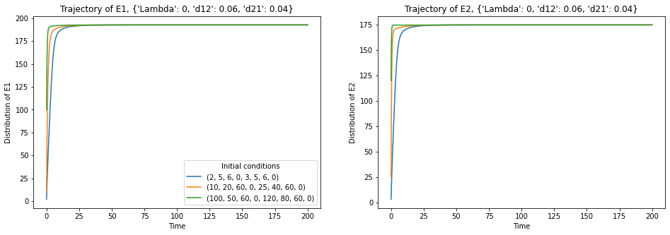
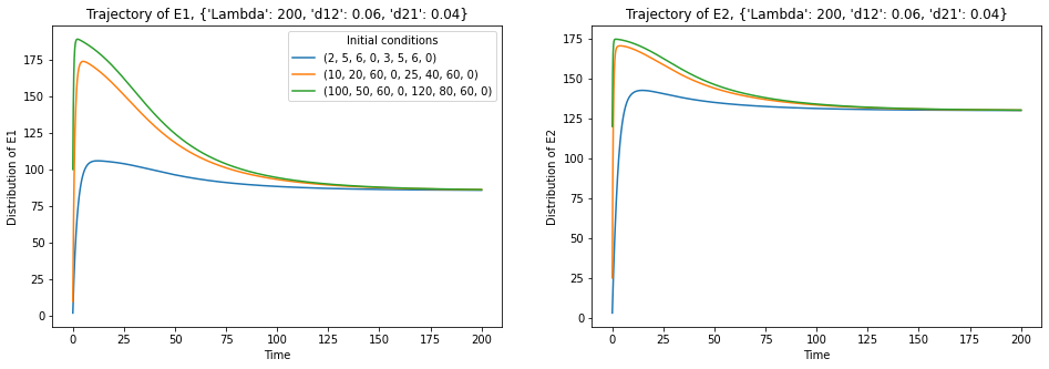
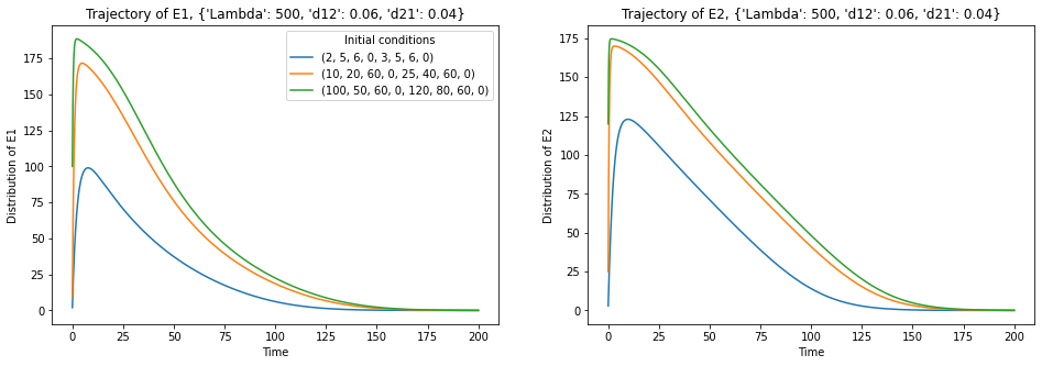
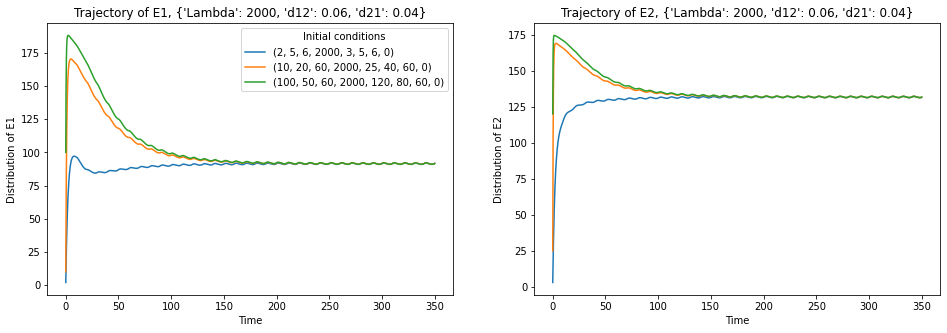
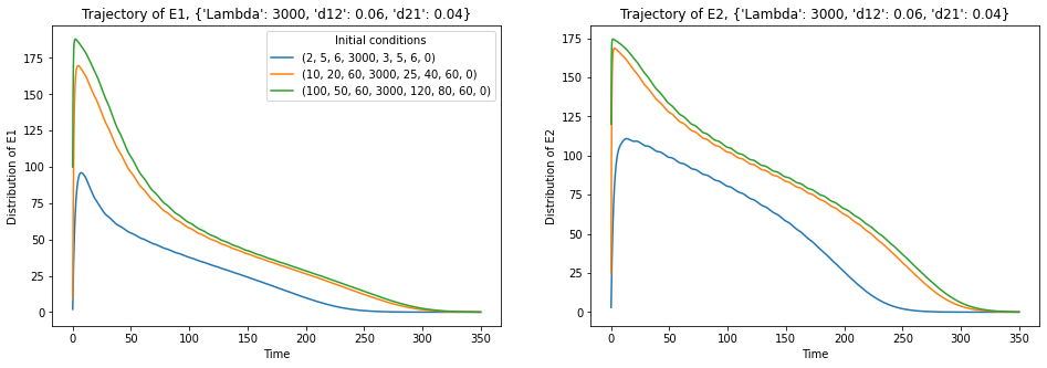
We take three different constant values of (). The initial density of sterile males is equal to zero. We approximate the positive equilibria in each case and plot the trajectories of and in Figures 3 according to different values of . We observe the following:
-
•
When , there is one positive equilibrium
All positive trajectories converge to the positive steady state .
-
•
When (), there are two positive equilibria
All positive trajectories also converge to the larger positive steady state .
-
•
When (), there is no positive equilibrium. All the trajectories converge to the zero equilibrium.
This validates the result in Theorem 4.2 that when exceeds some critical value, zero is the unique equilibrium of system (1). The observation for illustrates the result in Theorem 3.1 that there is one positive equilibrium and it is globally asymptotically stable. The introduction of sterile males () reduces the value of the positive steady state (see Figure 3(b)), and when () exceeds some critical value (at most equal to 500), all trajectories converge to the zero equilibrium (see Figure 3(c)). This illustrates the first point of Theorem 4.2. To approximate the critical value of , we provide some numerical bifurcation diagrams in Section 6.2.
6.1.2 Periodic impulsive releases
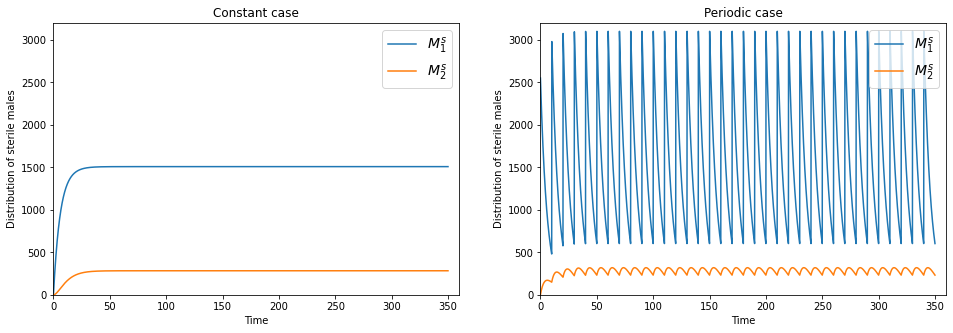
In this part, we consider the periodic impulsive releases with defined in (18), with equal to and (), the period (days). The trajectories of shown in Figure 4 converge to the periodic solution when () and go to zero when (). This illustrates the second point of Theorem 4.2 that when the number of sterile males released exceeds a critical value , the wild populations of mosquitoes in both areas reach elimination.
6.2 Critical values and bifurcation
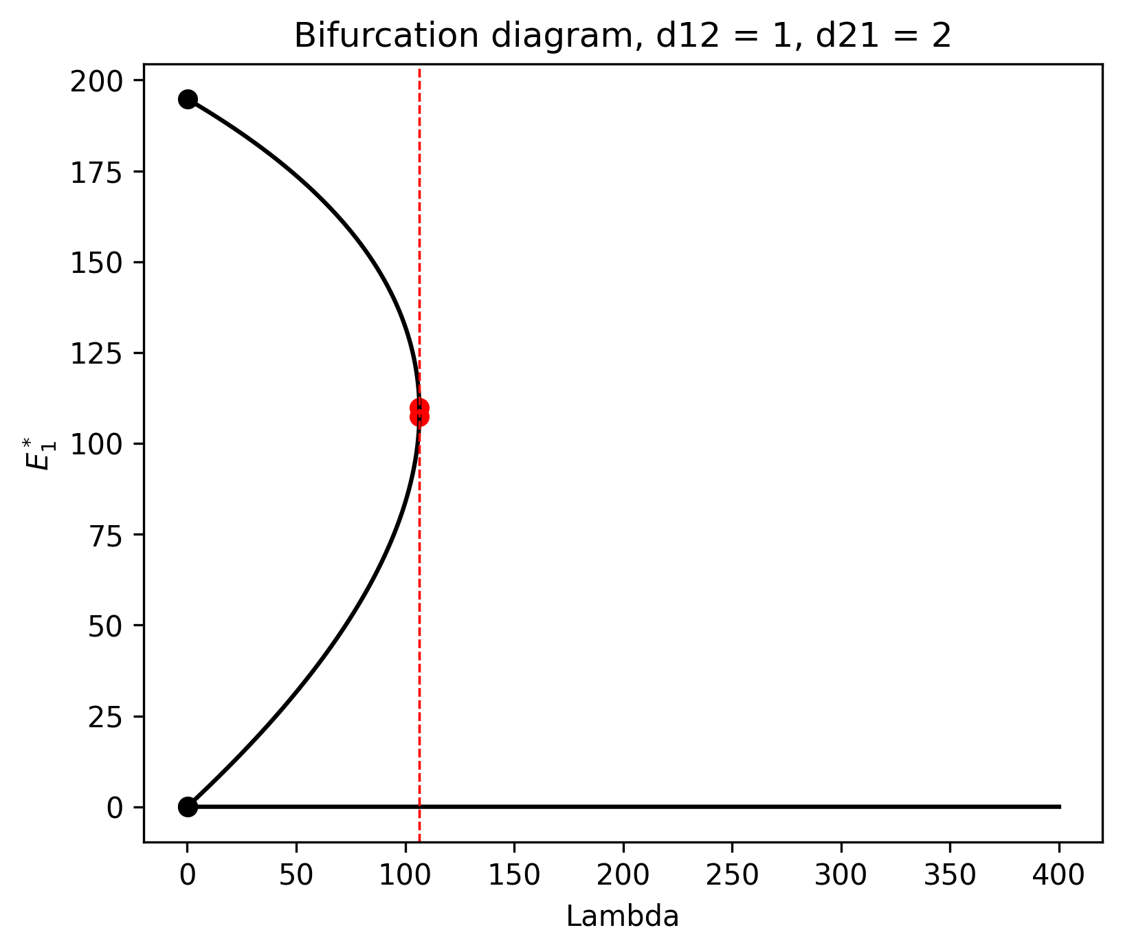
Our aim in this section is to approximate the critical value of where the bifurcation occurs.
6.2.1 Bifurcation diagram in the constant release case
We solve a system of nonlinear stationary problem for all values of the parameter , knowing that the solutions are continuous with respect to . Solving by numerical approximations can be done using numerical continuation methods (see [32]).
Here we present the simplest method called Natural Parameter Continuation (incremental methods, see [32]): Iteratively find approximate roots of for several values of with index . The root of step is used as an initial guess for the numerical solver at step . The first initial guess is the root for the smallest . To approximate the critical value in the constant case and examine what happens when , we draw the bifurcation diagram for . The initial positions of the numerical continuation are taken at the approximated equilibria when .
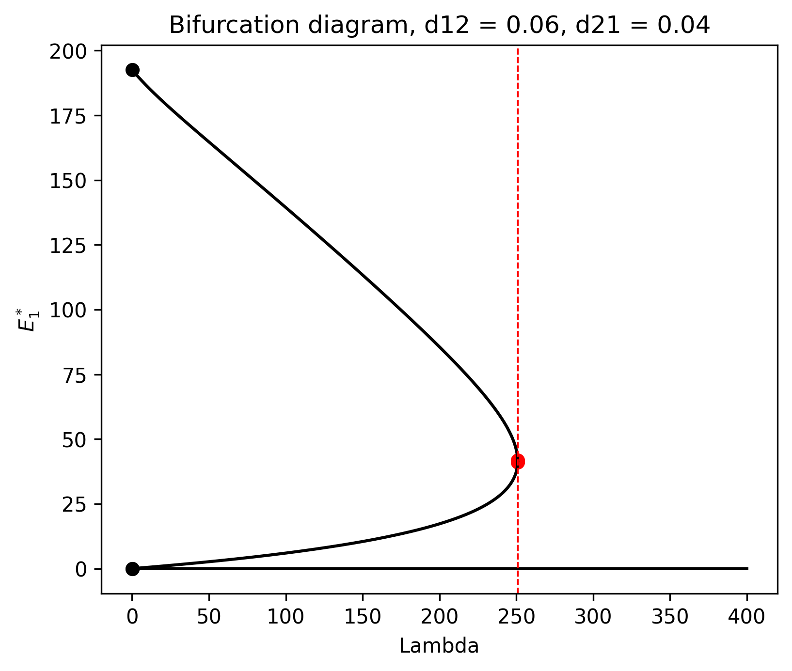
We obtain the bifurcation diagrams in Figure 5 for two scenarios. We observed that the critical value of decreases when the diffusion rates increase.
-
•
For , the critical value ().
-
•
For , the critical value ().
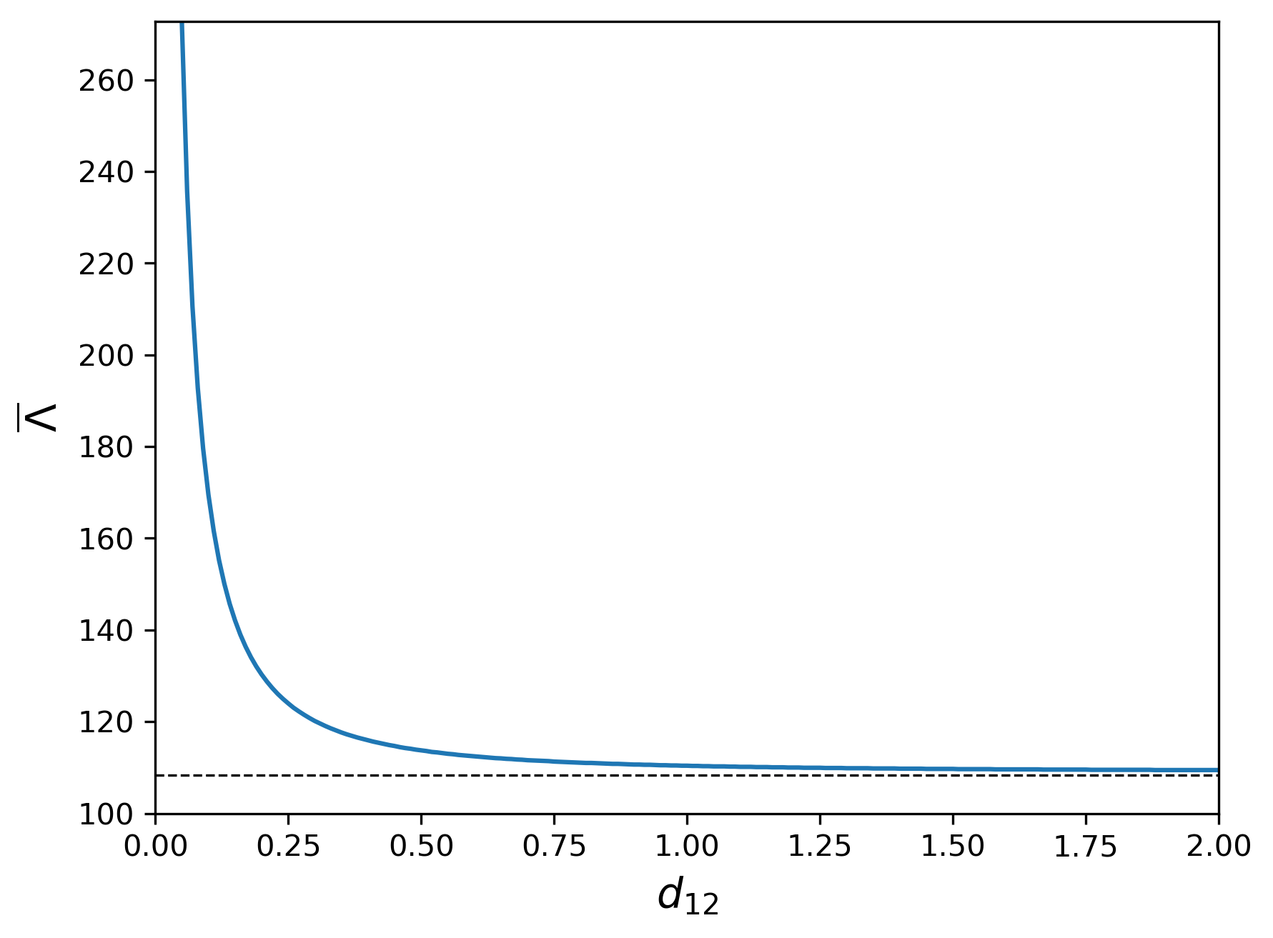
Taking , we plot the critical value corresponding to the moving rates (see Figure 6). This shows that the value of decreases when the diffusion rate gets larger, and converges to a value () as goes to infinity. This validates the result provided by Proposition 5.2 where is the critical value of corresponding to system (27). We also found that where is the critical value of the system when there is no separation between the two sub-populations defined in 5.1.2.
6.2.2 Comparison of release strategies
In practice, the strategy using impulsive releases is more realistic than the constant strategy. In this section, we make a comparison between these two strategies.
For the fixed diffusion rates , we approximated the critical number of sterile males released in both cases using the method in 6.2
-
•
When constant, the critical value ();
-
•
When with period , the critical value of is ().
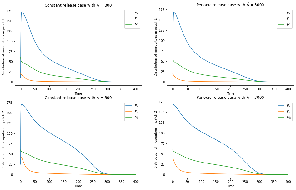
We can see that and are consistent. We also present numerical simulations in both cases with the same total amount of sterile males released where . The densities of sterile males in both cases are shown in Figure 7. We obtained in Figure 8 that in both cases, the wild mosquito population reaches elimination at time . Again we can see that the two strategies provide the same performance.
7 Discussion and conclusion
The existence of some hidden areas (e.g. crab burrows) that can not be accessed by the SIT hinders the population from reaching elimination. Without the implementation of this technique, Theorem 3.1 showed that the wild populations in both areas are persistent and converge towards the unique positive equilibrium (see Figure 3(a)) and are independent of the diffusion rates between them. The main results obtained in the present work indicated that with a sufficient number of sterile males released, the SIT succeeds in driving both sub-populations to extinction. We investigated both continuous constant releases and impulsive periodic releases in Theorem 4.2. The two strategies provided almost similar performance but the periodic release is more realistic in practice. The idea in our proof can also be used to design a feedback release strategy and this could be studied in future works.
The results also pointed out that the critical numbers of released sterile males are monotone with respect to the biological parameters of the population (see Section 5.2). A population with a larger birth rate of wild mosquitoes and a bigger carrying capacity of the environment requires more sterile males to reach elimination. A larger death rate in any compartment of the wild mosquitoes reduces this critical value, and on the contrary larger death rate for the sterile males increases this value.
Moreover, the critical number of sterile males also depends on the diffusion rates between the treated area and the inaccessible zone. More precisely, if the diffusion rates are large, this system approaches the case when there is no separation between two sub-populations (see Theorem 5.2). Numerically, we showed that the larger the values of diffusion rates, the smaller the threshold we need to exceed to obtain elimination (see Figure 6). This also showed that when the movement is at a low level, the leak of wild mosquitoes from the inaccessible area impedes the eradication in the treated zone and it requires a large number of sterile males to break through this obstacle. In practice, this could be an unrealistic amount of sterile mosquitoes. It is not surprising that the scenario with larger diffusion between two areas is better since more sterile males can arrive at the unreachable zone.
Acknowledgments
This study is supported by the STIC AmSud project BIO-CIVIP 23-STIC-02.
N. Nguyen has received funding from the European Union’s Horizon 2020 research and innovation program under the Marie Sklodowska-Curie grant agreement No 945332.
References
- [1] Abreu, F. V. S. d., Morais, M. M., Ribeiro, S. P., and Eiras, A. E. Influence of breeding site availability on the oviposition behaviour of Aedes aegypti. Memorias do Instituto Oswaldo Cruz 110 (July 2015), 669–676. Publisher: Instituto Oswaldo Cruz, Ministério da Saúde.
- [2] Achee, N. L., Grieco, J. P., Vatandoost, H., Seixas, G., Pinto, J., Ching-NG, L., Martins, A. J., Juntarajumnong, W., Corbel, V., Gouagna, C., David, J.-P., Logan, J. G., Orsborne, J., Marois, E., Devine, G. J., and Vontas, J. Alternative strategies for mosquito-borne arbovirus control. PLOS Neglected Tropical Diseases 13, 1 (Jan. 2019), e0006822. Publisher: Public Library of Science.
- [3] Allen, L. J. S. Persistence, extinction, and critical patch number for island populations. Journal of Mathematical Biology 24, 6 (Feb. 1987), 617–625.
- [4] Almeida, L., Estrada, J., and Vauchelet, N. Wave blocking in a bistable system by local introduction of a population: application to sterile insect techniques on mosquito populations. Mathematical Modelling of Natural Phenomena 17 (2022), 22. Publisher: EDP Sciences.
- [5] Almeida, L., Leculier, A., Nguyen, N., and Vauchelet, N. Rolling carpet strategies to eliminate mosquitoes: two-dimensional case. (paper in preparation), 2023.
- [6] Almeida, L., Léculier, A., and Vauchelet, N. Analysis of the Rolling Carpet Strategy to Eradicate an Invasive Species. SIAM Journal on Mathematical Analysis 55, 1 (Feb. 2023), 275–309. Publisher: Society for Industrial and Applied Mathematics.
- [7] Anguelov, R., Dumont, Y., and Lubuma, J. Mathematical modeling of sterile insect technology for control of anopheles mosquito. Computers & Mathematics with Applications 64, 3 (Aug. 2012), 374–389.
- [8] Anguelov, R., Dumont, Y., and Yatat Djeumen, I. V. Sustainable vector/pest control using the permanent sterile insect technique. Mathematical Methods in the Applied Sciences 43, 18 (2020), 10391–10412. _eprint: https://onlinelibrary.wiley.com/doi/pdf/10.1002/mma.6385.
- [9] Auger, P., Kouokam, E., Sallet, G., Tchuente, M., and Tsanou, B. The Ross–Macdonald model in a patchy environment. Mathematical Biosciences 216, 2 (Dec. 2008), 123–131.
- [10] Becker, N., Petrić, D., Zgomba, M., Boase, C., Madon, M. B., Dahl, C., and Kaiser, A. Mosquitoes: Identification, Ecology and Control. Fascinating Life Sciences. Springer International Publishing, Cham, 2020.
- [11] Bliman, P.-A., Cardona-Salgado, D., Dumont, Y., and Vasilieva, O. Implementation of control strategies for sterile insect techniques. Mathematical Biosciences 314 (Aug. 2019), 43–60.
- [12] Bliman, P.-A., and Dumont, Y. Robust control strategy by the Sterile Insect Technique for reducing epidemiological risk in presence of vector migration. Mathematical Biosciences 350 (Aug. 2022), 108856.
- [13] Bonnet, D. D., and Chapman, H. The larval habitats of Aedes polynesiensis Marks in Tahiti and methods of control. American Journal of Tropical Medicine and Hygiene 7, 5 (1958). Publisher: Baltimore, Md.
- [14] Chaplygin, S. Selected works on mechanics and mathematics. State Publ. House, Technical-Theoretical Literature, Moscow (1954).
- [15] Chaves, L. F., Hamer, G. L., Walker, E. D., Brown, W. M., Ruiz, M. O., and Kitron, U. D. Climatic variability and landscape heterogeneity impact urban mosquito diversity and vector abundance and infection. Ecosphere 2, 6 (2011), art70. _eprint: https://onlinelibrary.wiley.com/doi/pdf/10.1890/ES11-00088.1.
- [16] Coppel, W. A. Stability and Asymptotic Behavior of Differential Equations. Heath, 1965.
- [17] Dufourd, C., and Dumont, Y. Impact of environmental factors on mosquito dispersal in the prospect of sterile insect technique control. Computers & Mathematics with Applications 66, 9 (Nov. 2013), 1695–1715.
- [18] Dumont, Y., and Tchuenche, J. M. Mathematical studies on the sterile insect technique for the Chikungunya disease and Aedes albopictus. Journal of Mathematical Biology 65, 5 (Nov. 2012), 809–854.
- [19] Dyck, V. A., Hendrichs, J., and Robinson, A. S., Eds. Sterile Insect Technique: Principles and Practice in Area-Wide Integrated Pest Management, 2 ed. CRC Press, Boca Raton, Jan. 2021.
- [20] Heath, K., Bonsall, M. B., Marie, J., and Bossin, H. C. Mathematical modelling of the mosquito Aedes polynesiensis in a heterogeneous environment. Mathematical Biosciences 348 (June 2022), 108811.
- [21] Knipling, E. F. Sterile-Male Method of Population Control. Science 130, 3380 (Oct. 1959), 902–904. Publisher: American Association for the Advancement of Science.
- [22] Lardeux, F., Riviere, F., Sechan, Y., and Kay, B. H. Release of Mesocyclops aspericornis (Copepoda) for Control of Larval Aedes polynesiensis (Diptera: Culicidae) in Land Crab Burrows on an Atoll of French Polynesia. Journal of Medical Entomology 29, 4 (July 1992), 571–576.
- [23] Lardeux, F., Sechan, Y., and Faaruia, M. Evaluation of Insecticide Impregnated Baits for Control of Mosquito Larvae in Land Crab Burrows on French Polynesian Atolls. Journal of Medical Entomology 39, 4 (July 2002), 658–661.
- [24] Leculier, A., and Nguyen, N. A control strategy for the sterile insect technique using exponentially decreasing releases to avoid the hair-trigger effect. Mathematical Modelling of Natural Phenomena 18 (2023), 1–25. Publisher: EDP Sciences.
- [25] Lewis, M. A., and Van Den Driessche, P. Waves of extinction from sterile insect release. Mathematical Biosciences 116, 2 (Aug. 1993), 221–247.
- [26] Li, M. Y., and Shuai, Z. Global-stability problem for coupled systems of differential equations on networks. Journal of Differential Equations 248, 1 (Jan. 2010), 1–20.
- [27] Lu, Z., and Takeuchi, Y. Global asymptotic behavior in single-species discrete diffusion systems. J. Math. Biol. 32, 1 (Nov. 1993), 67–77.
- [28] Lutambi, A. M., Penny, M. A., Smith, T., and Chitnis, N. Mathematical modelling of mosquito dispersal in a heterogeneous environment. Mathematical Biosciences 241, 2 (Feb. 2013), 198–216.
- [29] Mann Manyombe, M. L., Tsanou, B., Mbang, J., and Bowong, S. A metapopulation model for the population dynamics of anopheles mosquito. Applied Mathematics and Computation 307 (Aug. 2017), 71–91.
- [30] Manoranjan, V. S., and Van Den Driessche, P. On a diffusion model for sterile insect release. Mathematical Biosciences 79, 2 (June 1986), 199–208.
- [31] Martens, P., and Hall, L. Malaria on the move: human population movement and malaria transmission. Emerging Infectious Diseases 6, 2 (2000), 103–109.
- [32] Rheinboldt, W. C. Numerical continuation methods: a perspective. Journal of Computational and Applied Mathematics 124, 1 (Dec. 2000), 229–244.
- [33] Smith, H. Monotone Dynamical Systems: An Introduction to the Theory of Competitive and Cooperative Systems, vol. 41 of Mathematical Surveys and Monographs. American Mathematical Society, Providence, Rhode Island, Mar. 2008.
- [34] Stoddard, S. T., Forshey, B. M., Morrison, A. C., Paz-Soldan, V. A., Vazquez-Prokopec, G. M., Astete, H., Reiner, R. C., Vilcarromero, S., Elder, J. P., Halsey, E. S., Kochel, T. J., Kitron, U., and Scott, T. W. House-to-house human movement drives dengue virus transmission. Proceedings of the National Academy of Sciences 110, 3 (Jan. 2013), 994–999. Publisher: Proceedings of the National Academy of Sciences.
- [35] Strugarek, M., Bossin, H., and Dumont, Y. On the use of the sterile insect release technique to reduce or eliminate mosquito populations. Applied Mathematical Modelling 68 (Apr. 2019), 443–470.
- [36] Takeuchi, Y. Cooperative Systems Theory and Global Stability of Diffusion Models. In Evolution and Control in Biological Systems (Dordrecht, 1989), A. B. Kurzhanski and K. Sigmund, Eds., Springer Netherlands, pp. 49–57.
- [37] Global vector control response 2017-2030., 2017. World Health Organization.
- [38] Yang, C., Zhang, X., and Li, J. Dynamics of two-patch mosquito population models with sterile mosquitoes. Journal of Mathematical Analysis and Applications 483, 2 (Mar. 2020), 123660.