Non-invertible symmetries act locally by quantum operations

Abstract

Non-invertible symmetries of quantum field theories and many-body systems generalize the concept of symmetries by allowing non-invertible operations in addition to more ordinary invertible ones described by groups. The aim of this paper is to point out that these non-invertible symmetries act on local operators by quantum operations, i.e. completely positive maps between density matrices, which form a natural class of operations containing both unitary evolutions and measurements and play an important role in quantum information theory. This observation will be illustrated by the Kramers–Wannier duality of the one-dimensional quantum Ising chain, which is a prototypical example of non-invertible symmetry operations.

I Introduction

In recent years, the concept of symmetries has received generalization in various directions in the theoretical study of quantum field theories and of condensed-matter systems. One such generalization is to allow certain non-invertibility in the symmetry operations involved, and the resulting structure is now known under the name of non-invertible symmetries and is an active area of research. Important examples of such operations have been known for decades before this fashionable name was coined, however, and the most prototypical one is the Kramers–Wannier duality transformation $\mathsf{D}$ of the Ising model. This transformation commutes with the Hamiltonian at criticality, and as such plays a role analogous to ordinary symmetry operations. That said, it does not quite square to one but rather satisfies

$$\mathsf{D}^{2}=1+\mathsf{g}$$ (1)

where $\mathsf{g}$ is the $\mathbb{Z}_{2}$ symmetry of the Ising model, as explained in great detail e.g. in various works Hauru:2015abi ; Aasen:2016dop ; Li:2023ani ; Seiberg:2023cdc ; Seiberg:2024gek .

There is a conceptual question, however. Ordinary invertible symmetries are implemented by unitary transformations. When we say we allow non-invertible symmetry operations, exactly which class of operations do we allow ourselves to use?

The aim of this letter is to answer this question, by pointing out that they act locally by quantum operations, a notion prominent in quantum information theory and in the analysis of open quantum systems. Here, quantum operations form a natural class of processes which can be performed on quantum systems, including unitary evolutions, measurements, the introduction of ancillary degrees of freedom and tracing them out, and so on. They are defined to be linear transformations which map density matrices to density matrices. As such, they have to satisfy a certain positivity property, known under the name of complete positivity. Details on these notions can be found e.g. in Nielsen_Chuang .

Before proceeding, we note that this answer was actually already given in the context of two-dimensional continuum conformal field theory treated using von Neumann algebras in a series of works by Bischoff and collaborators Bischoff1 ; Bischoff2 ; Bischoff3 ; Bischoff4 ; Bischoff5 , but the discussions there unfortunately use mathematical notions unfamiliar to many of theoretical physicists. Here we would like to demonstrate that this observation holds much more generally in a language more understandable to us. We also note that the answer was practically known in the case of one-dimensional spin chains to the authors of Lootens:2023wnl , in which it was shown that any non-invertible symmetry operation can be realized by unitary quantum circuits and measurements, based on their formulation of dualities as matrix product operators Lootens:2021tet ; Lootens:2022avn . As such, the authors do not claim much originality in this letter; rather, the intention of the authors is to disseminate this important observation to a wider audience of physicists.

The rest of the letter is organized as follows. We first give a brief review of quantum operations and non-invertible symmetries, and then provide a very general argument that non-invertible symmetries act on local operators by quantum operations. As the argument would be rather abstract, we will then illustrate the idea concretely using the case of the Kramers–Wannier duality transformation of the one-dimensional quantum Ising chain. We will conclude with a number of remarks.

II Generalities

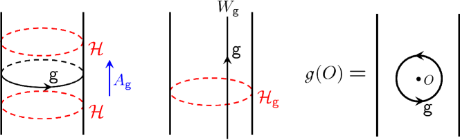
(a)

(b)

Figure 1: 1 Symmetry actions as walls in space (shown horizontally) and time (shown vertically). From left to right: as an action on the Hilbert space of states, as a wall implementing a twisted boundary condition, and as an operation on local operators. 1 Fusion of two $\mathsf{D}$ walls, here represented as actions on the Hilbert space of states.

II.1 Quantum operations

We start by recalling the concept of quantum operations. We will be brief; for details, the readers are referred to the standard textbooks, such as Nielsen_Chuang . Given a density matrix $\rho$ describing a quantum system with the Hilbert space $\mathcal{H}$, we consider an operation of the form $\rho\mapsto\rho^{\prime}=\mathcal{E}(\rho)$. First, to preserve the statistical interpretation of density matrices, we require that $\mathcal{E}(s\rho_{1}+(1-s)\rho_{2})=s\mathcal{E}(\rho_{1})+(1-s)\mathcal{E}(\rho_{2})$. This motivates us to define $\mathcal{E}$ as a linear map on the space of operators on $\mathcal{H}$. Second, density matrices $\rho$ have positive eigenvalues; such operators are called positive operators. Then, $\mathcal{E}$ should map positive operators to positive operators; such maps are called positive maps. Now, the operation $\mathcal{E}$ also acts naturally on operators on the enlarged Hilbert space $\mathcal{H}\otimes\mathbb{C}^{N}$, where $\mathbb{C}^{N}$ describes decoupled auxiliary degrees of freedom. We require that $\mathcal{E}$ should act on operators on $\mathcal{H}\otimes\mathbb{C}^{N}$ positively for all $N$; such an $\mathcal{E}$ is called a completely positive map. Quantum operations are then defined to be completely positive maps on operators on a Hilbert space $\mathcal{H}$; these operations include both unitary evolutions and measurements, and are also called as quantum channels, depending on the subfield of physics.

A natural subclass of quantum operations is defined by the condition that $\mathop{\mathrm{tr}}\mathcal{E}(\rho)=\mathop{\mathrm{tr}}\rho$, meaning that $\mathcal{E}$ preserves the total probability and describes the entire outcome of an operation rather than a specific subset. Such a completely positive map is called trace-preserving.

So far we used the Schrödinger picture where the operation $\mathcal{E}$ acts on the density matrices. We can instead use the Heisenberg picture and think of the operation as acting on observables as $O\mapsto\mathcal{E}^{\#}(O)$, by postulating $\mathop{\mathrm{tr}}\mathcal{E}^{\#}(O)\rho=\mathop{\mathrm{tr}}O\mathcal{E}(\rho)$. This $\mathcal{E}^{\#}$ is also completely positive. When $\mathcal{E}$ is trace-preserving, $\mathcal{E}^{\#}$ satisfies the condition $\mathcal{E}^{\#}(1)=1$ and is called a unital map. In the rest of the paper we always use the Heisenberg picture and we drop the superscript ^# from the notation. For convenience, we will slightly weaken the unital condition to allow a scalar-multiple: $\mathcal{E}(1)\propto 1$.

Any quantum operation $\mathcal{E}$ on operators on $\mathcal{H}$ is known to be represented as the combination of (i) introduction of an ancillary Hilbert space $\mathcal{H}^{\prime}$, (ii) a unitary evolution on the combined system $\mathcal{H}\otimes\mathcal{H}^{\prime}$, and (iii) removal of the ancillary Hilbert space $\mathcal{H}^{\prime}$ by a measurement or by the partial trace. When we regard $\mathcal{H}^{\prime}$ as the environment, this can be interpreted as describing the noise introduced by the environment; when we regard $\mathcal{H}^{\prime}$ as the measurement device, this procedure gives the effect of a measurement onto the target system.

More generally, we can use an entirely different Hilbert space $\mathcal{H}^{\prime\prime}$, a linear map $V:\mathcal{H}\to\mathcal{H}^{\prime\prime}$, and a representation $\pi$ of the algebra of operators on $\mathcal{H}^{\prime\prime}$. Then the combination $\mathcal{E}(O):=V^{\dagger}\pi(O)V$ is a quantum operation, and this form is known as the Stinespring representation of $\mathcal{E}$.

II.2 Non-invertible symmetries

Let us next review the concept of non-invertible symmetries. Again we will be very brief; more details can be found in various lecture notes, e.g. Schafer-Nameki:2023jdn ; Brennan:2023mmt ; Bhardwaj:2023kri ; Luo:2023ive ; Shao:2023gho ; Carqueville:2023jhb . An ordinary symmetry operation $\mathsf{g}$ of a quantum system described by a Hilbert space $\mathcal{H}$ is given by a unitary operator $A_{\mathsf{g}}$ on it. When $\mathsf{g}$ acts locally in a many-body or quantum field theory setting, we can consider a wall $W_{\mathsf{g}}$ in space, across which we twist the system by $\mathsf{g}$. For a system on a circle with one such wall, this represents a twisted boundary condition. The resulting Hilbert space is the twisted one $\mathcal{H}_{\mathsf{g}}$. The action of $A_{\mathsf{g}}$ can also be considered as the insertion of a wall in spacetime, spread along the spatial direction. Then the action $\mathdutchcal{g}(O)$ of $\mathsf{g}$ on an operator $O$ supported in a region of the space is given by wrapping the wall $W_{\mathsf{g}}$ around the operator, which is equivalent to $A_{\mathsf{g}}^{\dagger}OA_{\mathsf{g}}$. See Fig. 1 for an illustration of the discussions so far.

One important feature of these walls is that they can be freely moved in space and time as long as they do not hit other operators. Another feature is that they fuse according to the group law, $W_{\mathsf{g}\mathsf{h}}=W_{\mathsf{g}}W_{\mathsf{h}}$, and as such they are invertible: $W_{\mathsf{g}}W_{\mathsf{g}^{-1}}=1$. These two features are independent, and non-invertible symmetries are obtained by dropping the second property.

A prototypical example of non-invertible symmetry operations is the Kramers–Wannier duality transformation of the Ising model. In the language of the one-dimensional quantum Ising chain, this transformation exchanges the Hamiltonians $\sum_{i}(aX_{i}+bZ_{i}Z_{i+1})$ and $\sum_{i^{\prime}}(bX_{i^{\prime}}+aZ_{i^{\prime}}Z_{i^{\prime}+1})$. The operator $A_{\mathsf{D}}$ implementing this exchange on a closed chain however does not square to identity, and is known to satisfy $A_{\mathsf{D}}^{\dagger}A_{\mathsf{D}}=1+A_{\mathsf{g}}$, where $A_{\mathsf{g}}=\prod_{i}X_{i}$ is the $\mathbb{Z}_{2}$ symmetry operation. As we will review in more detail below, this duality transformation can be implemented locally on the Ising chain. Correspondingly, we can consider the duality wall $W_{\mathsf{D}}$ which fuses according to the rule $W_{\mathsf{D}^{\dagger}}W_{\mathsf{D}}=1+W_{\mathsf{g}}$. See Fig. 1 for an illustration of the ideas described here. Note that the action $\mathcal{D}(O)$ of a non-invertible symmetry $\mathsf{D}$ on an operator $O$, implemented by wrapping the wall $W_{\mathsf{D}}$ around the operator, is no longer equivalent to $A_{\mathsf{D}}^{\dagger}OA_{\mathsf{D}}$.

II.3 Non-invertible symmetries act locally by quantum operations

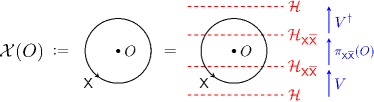
Figure 2: Action of a non-invertible symmetry $\mathsf{X}$ on a local operator $O$, making it manifest that it is a Stinespring representation of a completely positive map.

We are now able to demonstrate our main claim that non-invertible symmetries act locally by quantum operations. The demonstration is surprisingly simple and general, see Fig. 2. Consider the action of a non-invertible symmetry operation $\mathcal{X}$ on an operator $O$ acting on $\mathcal{H}$. As shown in the figure, we first go from the original Hilbert space $\mathcal{H}$ to the Hilbert space $\mathcal{H}_{\mathsf{X}\overline{\mathsf{X}}}$ with a wall $W_{\mathsf{X}}$ and another wall $W_{\overline{\mathsf{X}}}$ inserted, by a linear map $V$. We then act by the operator $O$ on $\mathcal{H}_{\mathsf{X}\overline{\mathsf{X}}}$, which we denote by $\pi_{\mathsf{X}\overline{\mathsf{X}}}(O)$. We now come back to the original Hilbert space $\mathcal{H}$ by $V^{\dagger}$. Then we find

$$\mathcal{X}(O)=V^{\dagger}\pi_{\mathsf{X}\overline{\mathsf{X}}}(O)V,$$ (2)

which is precisely a Stinespring representation of a completely positive map. This argument is very general, and does not assume whether the theory is defined in continuum or on a lattice. It does not assume that we have tensor-product Hilbert spaces either. The argument is admittedly very abstract, however. We will now make it more concrete by studying the case of the Kramers–Wannier duality wall explicitly.

III Kramers–Wannier duality

We consider a one-dimensional spin chain, with each site $\bullet$ described by a qubit $\ket{0}$, $\ket{1}$ spanning a Hilbert space $\mathcal{H}(\bullet)=\mathbb{C}^{2}$. We use $X$, $Y$, $Z$ to denote the Pauli matrices acting on the qubit. We consider the $\mathbb{Z}_{2}$ symmetry $\mathsf{g}$ acting on the qubit by $X$.

We take the convention that the wall ${\mid}$ implementing $\mathsf{g}$ sits in between two sites as in $\cdots\bullet{\bullet}{{\mid}}{\bullet}\bullet\cdots$. The Hilbert space for this chain will be denoted as $\mathcal{H}(\cdots\bullet_{i}{\mid}\bullet_{i+1}\cdots)$; then the motion of the wall by one unit is given by

$$\mathcal{H}(\cdots{\mid}\bullet_{i}\cdots)\xrightarrow{R_{\mathsf{g},i}:=X_{i}}\mathcal{H}(\cdots\bullet_{i}{\mid}\cdots),$$ (3)

and the insertion of two walls at the same place is a trivial operation:

$$\mathcal{H}(\cdots\bullet_{i}\bullet_{i+1}\cdots)\xrightarrow{V_{\mathsf{g}\overline{\mathsf{g}},i}:=\mathrm{id}}\mathcal{H}(\cdots\bullet_{i}{\mid}{\mid}\bullet_{i+1}\cdots).$$ (4)

Let $O$ be an operator supported on the sites from $j$ to $k$, with $j<k$. Our definition leads to the local action of $\mathsf{g}$ given by

$$\mathdutchcal{g}(O)=(X_{k}X_{k-1}\cdots X_{j})O(X_{j}^{\dagger}\cdots X_{k-1}^{\dagger}X_{k}^{\dagger}),$$ (5)

exactly as expected.

Let us next discuss the wall implementing the Kramers–Wannier duality $\mathsf{D}$, which was already studied in great detail in Hauru:2015abi ; Aasen:2016dop ; Li:2023ani ; Seiberg:2023cdc ; Seiberg:2024gek . We take the convention that the wall sits on top of a site, as in $\cdots\bullet\ooalign{\hfil$\bullet$\hfil\cr\hfil$\vbox{\hbox{ \leavevmode\hbox to1.54pt{\vbox to14.63pt{\text{[drawing]}}}}}$\hfil\cr}\bullet\cdots$. Then the motion of the wall to the right by one unit is given by

$$\mathcal{H}(\cdots\ooalign{\hfil$\bullet$\hfil\cr\hfil$\vbox{\hbox{ \leavevmode\hbox to1.54pt{\vbox to14.63pt{\text{[drawing]}}}}}$\hfil\cr}_{i}\bullet_{i+1}\cdots)\xrightarrow{R_{\mathsf{D},i+1}:=U^{H}_{i+1}U^{CZ}_{i,i+1}}\mathcal{H}(\cdots\bullet_{i}\ooalign{\hfil$\bullet$\hfil\cr\hfil$\vbox{\hbox{ \leavevmode\hbox to1.54pt{\vbox to14.63pt{\text{[drawing]}}}}}$\hfil\cr}_{i+1}\cdots),$$ (6)

where $U^{CZ}$ acts on two qubits by the controlled-$Z$ gate

$$\bra{s^{\prime}t^{\prime}}U^{CZ}\ket{st}=\delta^{s^{\prime}}_{s}\delta^{t^{\prime}}_{t}(-1)^{st},$$ (7)

and $U^{H}$ acts on a single qubit by the Hadamard gate

$$\bra{t^{\prime}}U^{H}\ket{t}=\sqrt{2}^{-1}(-1)^{t^{\prime}t}.$$ (8)

Two walls are introduced by the following operation:

$$\begin{array}[]{cccc}V_{\mathsf{D}\overline{\mathsf{D}},i}\colon&\mathcal{H}(\cdots\bullet_{i}\bullet_{i+1}\cdots)&\xrightarrow{\otimes\ket{0_{a}}}\mathcal{H}(\cdots\bullet_{i}\ooalign{\hfil$\bullet$\hfil\cr\hfil$\vbox{\hbox{ \leavevmode\hbox to1.54pt{\vbox to14.63pt{\text{[drawing]}}}}}\vbox{\hbox{ \leavevmode\hbox to1.54pt{\vbox to14.63pt{\text{[drawing]}}}}}$\hfil\cr}_{a}\bullet_{i+1}\cdots)\xrightarrow{R_{\mathsf{D},a}^{\dagger}}&\mathcal{H}(\cdots\ooalign{\hfil$\bullet$\hfil\cr\hfil$\vbox{\hbox{ \leavevmode\hbox to1.54pt{\vbox to14.63pt{\text{[drawing]}}}}}$\hfil\cr}_{i}\ooalign{\hfil$\bullet$\hfil\cr\hfil$\vbox{\hbox{ \leavevmode\hbox to1.54pt{\vbox to14.63pt{\text{[drawing]}}}}}$\hfil\cr}_{a}\bullet_{i+1}\cdots),\\ &\rotatebox{90.0}{$\in$}&&\rotatebox{90.0}{$\in$}\\[-4.30554pt] &\ket{\cdots s_{i}s_{i+1}\cdots}&\xmapsto{\phantom{verylongverylongindeedveryverylong}}&\sqrt{2}^{\frac{1}{2}}R_{\mathsf{D},a}^{\dagger}\ket{\cdots s_{i}0_{a}s_{i+1}\cdots}\end{array}$$ (18)

i.e. tensoring the state $\ket{0}_{a}\in\mathcal{H}(\ooalign{\hfil$\bullet$\hfil\cr\hfil$\vbox{\hbox{ \leavevmode\hbox to1.54pt{\vbox to14.63pt{\text{[drawing]}}}}}\vbox{\hbox{ \leavevmode\hbox to1.54pt{\vbox to14.63pt{\text{[drawing]}}}}}$\hfil\cr}_{a})$ of the ancillary qubit and detaching one of the walls to the left .

Again let $O$ be an operator supported well within the sites from $j$ to $k$, with $j<k$. Our definition leads to the local action of $\mathsf{D}$ given by

$$\mathcal{D}(O)=V_{\mathsf{D}\overline{\mathsf{D}},k}^{\dagger}(R_{\mathsf{D},k}R_{\mathsf{D},k-1}\cdots R_{\mathsf{D},j})\times\\ O(R_{\mathsf{D},j}^{\dagger}\cdots R_{\mathsf{D},k-1}^{\dagger}R_{\mathsf{D},k}^{\dagger})V_{\mathsf{D}\overline{\mathsf{D}},k}$$ (19)

For example, let

$$H=\sum_{i=j^{\prime}}^{k^{\prime}-1}(aX_{i}+bZ_{i}Z_{i+1})+aX_{k^{\prime}}$$ (20)

be the standard Hamiltonian of the Ising chain restricted to the sites $j^{\prime}$ to $k^{\prime}$. Assuming $j\leq j^{\prime}$ and $k^{\prime}\leq k$, we can use the formula above to compute the local action of $\mathsf{D}$, and we find

$$\mathcal{D}(H)=\sqrt{2}\left[\sum_{i=j^{\prime}}^{k^{\prime}-1}(aZ_{i-1}Z_{i}+bX_{i})+aZ_{k^{\prime}-1}Z_{k^{\prime}}\right],$$ (21)

as expected for a local action of Kramers–Wannier duality. With some efforts, we can show that

$$\mathcal{R}(\mathcal{D}^{2}(O))=O+\mathdutchcal{g}(O)$$ (22)

in general, where $\mathcal{R}$ is the operation to move an operator one unit to the right . For example, for $j<i<k$, we can easily check

$$\mathcal{D}(Z_{i})=0,$$ (23)

which is compatible with (22), as $\mathdutchcal{g}(Z_{i})=-Z_{i}$.

Before proceeding, we note that the implementation of Kramers–Wannier duality operation and broader classes of non-invertible symmetries by quantum circuits and measurements was discussed in many other places, e.g. Ashkenazi:2021ieg ; Tantivasadakarn:2021vel ; Lootens:2021tet ; Aasen:2022cdu ; Bravyi:2022zcw ; Tantivasadakarn:2022hgp ; Lootens:2022avn ; Lootens:2023wnl ; Fechisin:2023dkj ; Okuda:2024jzh .

IV Concluding Remarks

In this letter we gave a general argument that non-invertible symmetries act on locally-supported operators by quantum operations. We also illustrated this observation in the concrete case of the Kramers–Wannier duality of the one-dimensional quantum Ising chain, where we can explicitly see the introduction of an ancillary qubit in a specific state, the action of unitary operator on the combined system, and then the removal of the ancillary qubit.

The authors admit that what they have here is simply a curious observation, and that it was already noted several years ago in the context of algebraic quantum field theory in Bischoff1 ; Bischoff2 ; Bischoff3 ; Bischoff4 ; Bischoff5 , and that it was essentially understood in the context of spin chains in Lootens:2023wnl ; Lootens:2021tet ; Lootens:2022avn . The author thinks that it was still worthwhile to spend a few pages to explain this observation in a language understandable to more theoretical physicists, especially because this observation might open a fruitful flow of ideas between two actively researched areas.

For example, we can ask what the Petz recovery map on the quantum operation side corresponds to, if any, on the side of non-invertible symmetries. Is it related to existence of the dual $\overline{\mathsf{X}}$ for any non-invertible operation $\mathsf{X}$ such that $\overline{\mathsf{X}}\mathsf{X}$ contains the identity? Another natural question is to ask if the property of a general quantum system, not necessarily associated to quantum field theory or quantum many-body systems, would be affected or constrained in any way by the existence of a non-invertible symmetry structure. For example, the existence of an ordinary symmetry often leads to degeneracy in the spectrum. Can we say anything interesting about the spectrum of a Hamiltonian, if it is assumed to be invariant under two quantum operations $\mathcal{D}$ and $\mathdutchcal{g}$ satisfying $\mathcal{D}^{2}=1+\mathdutchcal{g}$? The authors hope to come back to these questions in the future, and the authors would also welcome other researchers to do so.

V Acknowledgments

The authors thank Kotaro Kawasumi for asking exactly which class of operations non-invertible symmetries are; without his question this letter would never have been born. The authors also thank Kantaro Ohmori for discussions, and Shu-Heng Shao and Yunqin Zheng for comments on the draft. MO is supported by FoPM, WINGS Program of the University of Tokyo, JSPS Research Fellowship for Young Scientists, JSPS KAKENHI Grant Number JP23KJ0650. Additionally, MO and YT are supported in part by WPI Initiative, MEXT, Japan at Kavli IPMU, the University of Tokyo.

References

• (1) M. Hauru, G. Evenbly, W. W. Ho, D. Gaiotto, and G. Vidal, Topological Conformal Defects with Tensor Networks, Phys. Rev. B 94 (2016) 115125, arXiv:1512.03846 [cond-mat.str-el].
• (2) D. Aasen, R. S. K. Mong, and P. Fendley, Topological Defects on the Lattice I: the Ising Model, J. Phys. A 49 (2016) 354001, arXiv:1601.07185 [cond-mat.stat-mech].
• (3) L. Li, M. Oshikawa, and Y. Zheng, Noninvertible Duality Transformation Between Symmetry-Protected Topological and Spontaneous Symmetry Breaking Phases, Phys. Rev. B 108 (2023) 214429, arXiv:2301.07899 [cond-mat.str-el].
• (4) N. Seiberg and S.-H. Shao, Majorana Chain and Ising Model – (Non-Invertible) Translations, Anomalies, and Emanant Symmetries, SciPost Phys. 16 (2024) 064, arXiv:2307.02534 [cond-mat.str-el].
• (5) N. Seiberg, S. Seifnashri, and S.-H. Shao, Non-Invertible Symmetries and LSM-Type Constraints on a Tensor Product Hilbert Space, arXiv:2401.12281 [cond-mat.str-el].
• (6) M. A. Nielsen and I. L. Chuang, Quantum Computation and Quantum Information. Cambridge University Press, 2010.
• (7) M. Bischoff, Generalized orbifold construction for conformal nets, Rev. Math. Phys. 29 (2017) 1750002, arXiv:1608.00253 [math-ph].
• (8) M. Bischoff and K.-H. Rehren, The hypergroupoid of boundary conditions for local quantum observables, in Operator algebras and mathematical physics, vol. 80 of Adv. Stud. Pure Math., pp. 23–42. Math. Soc. Japan, Tokyo, 2019. arXiv:1612.02972 [math-ph].
• (9) M. Bischoff, S. Del Vecchio, and L. Giorgetti, Compact hypergroups from discrete subfactors, J. Funct. Anal. 281 (2021) 109004, arXiv:2007.12384 [math.OA].
• (10) M. Bischoff, S. Del Vecchio, and L. Giorgetti, Galois correspondence and Fourier analysis on local discrete subfactors, Ann. Henri Poincaré 23 (2022) 2979–3020, arXiv:2107.09345 [math.OA].
• (11) M. Bischoff, S. Del Vecchio, and L. Giorgetti, Quantum operations on conformal nets, Rev. Math. Phys. 35 (2023) 2350007, arXiv:2204.14105 [math.OA].
• (12) L. Lootens, C. Delcamp, D. Williamson, and F. Verstraete, Low-depth unitary quantum circuits for dualities in one-dimensional quantum lattice models, arXiv:2311.01439 [quant-ph].
• (13) L. Lootens, C. Delcamp, G. Ortiz, and F. Verstraete, Dualities in One-Dimensional Quantum Lattice Models: Symmetric Hamiltonians and Matrix Product Operator Intertwiners, PRX Quantum 4 (2023) 020357, arXiv:2112.09091 [quant-ph].
• (14) L. Lootens, C. Delcamp, and F. Verstraete, Dualities in One-Dimensional Quantum Lattice Models: Topological Sectors, PRX Quantum 5 (2024) 010338, arXiv:2211.03777 [quant-ph].
• (15) S. Schäfer-Nameki, ICTP Lectures on (Non-)Invertible Generalized Symmetries, Phys. Rept. 1063 (2024) 1–55, arXiv:2305.18296 [hep-th].
• (16) T. D. Brennan and S. Hong, Introduction to Generalized Global Symmetries in QFT and Particle Physics, arXiv:2306.00912 [hep-ph].
• (17) L. Bhardwaj, L. E. Bottini, L. Fraser-Taliente, L. Gladden, D. S. W. Gould, A. Platschorre, and H. Tillim, Lectures on Generalized Symmetries, Phys. Rept. 1051 (2024) 1–87, arXiv:2307.07547 [hep-th].
• (18) R. Luo, Q.-R. Wang, and Y.-N. Wang, Lecture Notes on Generalized Symmetries and Applications, Phys. Rept. 1065 (2024) 1–43, arXiv:2307.09215 [hep-th].
• (19) S.-H. Shao, What’s Done Cannot Be Undone: TASI Lectures on Non-Invertible Symmetry, arXiv:2308.00747 [hep-th].
• (20) N. Carqueville, M. Del Zotto, and I. Runkel, Topological defects, in Encyclopedia of Mathematical Physics, 2nd ed. 2024. arXiv:2311.02449 [math-ph]. In press.
• (21) There is a subtlety in the notation asubscriptfragmentsfragments 𝑎\ooalign{\hfil$\bullet$\hfil\cr\hfil$\vbox{\hbox{ \leavevmode\hbox to1.54pt{\vbox to14.63pt{\pgfpicture\makeatletter\hbox{\hskip 0.76906pt\lower-0.2pt\hbox to0.0pt{\pgfsys@beginscope\pgfsys@invoke{ }\definecolor{pgfstrokecolor}{rgb}{0,0,0}\pgfsys@color@rgb@stroke{0}{0}{0}\pgfsys@invoke{ }\pgfsys@color@rgb@fill{0}{0}{0}\pgfsys@invoke{ }\pgfsys@setlinewidth{0.4pt}\pgfsys@invoke{ }\nullfont\hbox to0.0pt{\pgfsys@beginscope\pgfsys@invoke{ }{{}} {}{{}}{} {}{} {}{{}{}}{}{}{}{{}}{{}}{{}{}}{{}{}}{{{{}{}{{}} }}{{}} {} }{{{{}{}{{}} }}{{}} {} }{{{{}{}{{}} }}{{}} {} }{{{{}{}{{}} }}{{}} {} }{{{{}{}{{}} }}{{}} {} }{{{{}{}{{}} }}{{}} {} }{{{{}{}{{}} }}{{}} {} }{{{{}{}{{}} }}{{}} {} }{{{{}{}{{}} }}{{}} {} }{{{{}{}{{}} }}{{}} {} }{{}{}}{{}{}}{{{{}{}{{}} }}{{}} {{{}}} } {}\pgfsys@moveto{0.0pt}{0.0pt}\pgfsys@lineto{-0.56906pt}{0.71132pt}\pgfsys@lineto{0.56906pt}{2.13396pt}\pgfsys@lineto{-0.56906pt}{3.5566pt}\pgfsys@lineto{0.56906pt}{4.97923pt}\pgfsys@lineto{-0.56906pt}{6.40187pt}\pgfsys@lineto{0.56906pt}{7.82451pt}\pgfsys@lineto{-0.56906pt}{9.24715pt}\pgfsys@lineto{0.56906pt}{10.66978pt}\pgfsys@lineto{-0.56906pt}{12.09242pt}\pgfsys@lineto{0.56906pt}{13.51506pt}\pgfsys@lineto{0.0pt}{14.22638pt}\pgfsys@stroke\pgfsys@invoke{ } \pgfsys@invoke{\lxSVG@closescope }\pgfsys@endscope{}{}{}\hss}\pgfsys@discardpath\pgfsys@invoke{\lxSVG@closescope }\pgfsys@endscope\hss}}\lxSVG@closescope\endpgfpicture}}}}\vbox{\hbox{ \leavevmode\hbox to1.54pt{\vbox to14.63pt{\pgfpicture\makeatletter\hbox{\hskip 0.76906pt\lower-0.2pt\hbox to0.0pt{\pgfsys@beginscope\pgfsys@invoke{ }\definecolor{pgfstrokecolor}{rgb}{0,0,0}\pgfsys@color@rgb@stroke{0}{0}{0}\pgfsys@invoke{ }\pgfsys@color@rgb@fill{0}{0}{0}\pgfsys@invoke{ }\pgfsys@setlinewidth{0.4pt}\pgfsys@invoke{ }\nullfont\hbox to0.0pt{\pgfsys@beginscope\pgfsys@invoke{ }{{}} {}{{}}{} {}{} {}{{}{}}{}{}{}{{}}{{}}{{}{}}{{}{}}{{{{}{}{{}} }}{{}} {} }{{{{}{}{{}} }}{{}} {} }{{{{}{}{{}} }}{{}} {} }{{{{}{}{{}} }}{{}} {} }{{{{}{}{{}} }}{{}} {} }{{{{}{}{{}} }}{{}} {} }{{{{}{}{{}} }}{{}} {} }{{{{}{}{{}} }}{{}} {} }{{{{}{}{{}} }}{{}} {} }{{{{}{}{{}} }}{{}} {} }{{}{}}{{}{}}{{{{}{}{{}} }}{{}} {{{}}} } {}\pgfsys@moveto{0.0pt}{0.0pt}\pgfsys@lineto{-0.56906pt}{0.71132pt}\pgfsys@lineto{0.56906pt}{2.13396pt}\pgfsys@lineto{-0.56906pt}{3.5566pt}\pgfsys@lineto{0.56906pt}{4.97923pt}\pgfsys@lineto{-0.56906pt}{6.40187pt}\pgfsys@lineto{0.56906pt}{7.82451pt}\pgfsys@lineto{-0.56906pt}{9.24715pt}\pgfsys@lineto{0.56906pt}{10.66978pt}\pgfsys@lineto{-0.56906pt}{12.09242pt}\pgfsys@lineto{0.56906pt}{13.51506pt}\pgfsys@lineto{0.0pt}{14.22638pt}\pgfsys@stroke\pgfsys@invoke{ } \pgfsys@invoke{\lxSVG@closescope }\pgfsys@endscope{}{}{}\hss}\pgfsys@discardpath\pgfsys@invoke{\lxSVG@closescope }\pgfsys@endscope\hss}}\lxSVG@closescope\endpgfpicture}}}}$\hfil\cr}_{a} of two 𝖣𝖣\mathsf{D} walls on the same site, in that separating the wall to the left is given by R𝖣subscriptsuperscript𝑅𝖣R^{\dagger}_{\mathsf{D}} but separating the wall to the right is not simply given by R𝖣subscript𝑅𝖣R_{\mathsf{D}}. The latter operation needs to be given by R𝖣,aR𝖣,i+1V𝖣𝖣¯,isubscript𝑅𝖣𝑎subscript𝑅𝖣𝑖1subscript𝑉𝖣¯𝖣𝑖R_{\mathsf{D},a}R_{\mathsf{D},i+1}V_{\mathsf{D}\overline{\mathsf{D}},i}, i.e.  we always have to use V𝖣𝖣¯subscript𝑉𝖣¯𝖣V_{\mathsf{D}\overline{\mathsf{D}}} when introducing or canceling two 𝖣𝖣\mathsf{D} walls. See Hauru:2015abi ; Aasen:2016dop ; Li:2023ani ; Seiberg:2023cdc ; Seiberg:2024gek for other conventions.
• (22) For example, we can easily check $\mathcal{D}(X_{i})=\sqrt{2}Z_{i-1}Z_{i}$ and $\mathcal{D}(\sqrt{2}Z_{i-1}Z_{i})=2X_{i-1}$ from (19). If we prefer not to have the appearance of the lattice translation here, we can consider $\mathcal{D}^{\prime}(O)$, which introduces two $\mathsf{D}$ walls at a site on the left of $j-1$, moves one wall to the right beyond $k+1$, acts $O$, and reverses the wall motion. Then $\mathcal{D}^{\prime}(\mathcal{D}(O))=O+\mathdutchcal{g}(O)$ follows. Another option is to use a convention that distinguishes spins and dual spins Aasen:2016dop ; Li:2023ani .
• (23) S. Ashkenazi and E. Zohar, Duality as a feasible physical transformation for quantum simulation, Phys. Rev. A 105 (2022) 022431, arXiv:2111.04765 [quant-ph].
• (24) N. Tantivasadakarn, R. Thorngren, A. Vishwanath, and R. Verresen, Long-range entanglement from measuring symmetry-protected topological phases, arXiv:2112.01519 [cond-mat.str-el]. Accepted in PRX.
• (25) D. Aasen, Z. Wang, and M. B. Hastings, Adiabatic paths of Hamiltonians, symmetries of topological order, and automorphism codes, Phys. Rev. B 106 (2022) 085122, arXiv:2203.11137 [quant-ph].
• (26) S. Bravyi, I. Kim, A. Kliesch, and R. Koenig, Adaptive constant-depth circuits for manipulating non-abelian anyons, arXiv:2205.01933 [quant-ph].
• (27) N. Tantivasadakarn, A. Vishwanath, and R. Verresen, Hierarchy of Topological Order From Finite-Depth Unitaries, Measurement, and Feedforward, PRX Quantum 4 (2023) 020339, arXiv:2209.06202 [quant-ph].
• (28) C. Fechisin, N. Tantivasadakarn, and V. V. Albert, Non-invertible symmetry-protected topological order in a group-based cluster state, arXiv:2312.09272 [cond-mat.str-el].
• (29) T. Okuda, A. Parayil Mana, and H. Sukeno, Anomaly inflow, dualities, and quantum simulation of abelian lattice gauge theories induced by measurements, arXiv:2402.08720 [cond-mat.str-el].