Existence and Uniqueness of Rayleigh waves with both normal and tangential boundary conditions
Abstract.
Impedance boundary condition are of great interest in linear elasticity as a method to model several non-standard problems. Recently, in the frame of surface wave propagation in an elastic isotropic half-space, Godoy et al. [Wave Motion 49 (2012), 585-594] proposed a general class of impedance boundary conditions that generalize the standard stress-free boundary condition in the non-dispersive regime. A natural question that arises in this context is whether the property of existence and uniqueness of a surface wave, observed in the stress-free case (called Rayleigh wave), holds for full Godoy’s impedance boundary conditions. Godoy et al. addressed this question for the tangential case (the tangential stress is proportional to the horizontal displacement times the frequency and the normal stress vanishes). Recently, Giang and Vinh [J Eng Math 130, 13 (2021)] studied the normal case (the tangential stress vanishes and the normal stress is proportional to the normal displacement times the frequency). In this work, we consider an uniparametric family of Godoy’s impedance boundary conditions defined by proportional ratios of the same magnitude but opposite sign. We demonstrate the existence and uniqueness of the Rayleigh surface wave for each value of the impedance parameter, showing for the first time that full Godoy’s impedance boundary conditions are also capable of explaining surface wave propagation. Numerical examples are presented to illustrate the effect of the impedance parameter in the speed of the surface wave.
Key words and phrases:
Rayleigh waves, impedance boundary conditions, secular equation, hyperbolic systems2020 Mathematics Subject Classification:
35Q74, 74B05, 74J20, 74J40, 35L051. Introduction
Rayleigh surface waves, originally described by Rayleigh [22] in 1885, have consistently drawn the interest of researchers due to their extensive applications across a wide range of scientific fields. Notably in seismology, where they have the potential to explain most of the damage and destruction during an earthquake. A lot of investigations on Rayleigh wave propagation on general anisotropic elastic half-space have been conducted, where the stress-free boundary condition constitutes the main paradigm (see, e.g., [22, 1, 17, 3, 33, 28]).
However recently, there has been an increasing interest on surface wave propagation under impedance boundary conditions, which are usually defined by linear relations between the unknown function and its derivatives at the surface. The usual stress-free boundary condition arises as a particular case. Although commonly used in electromagnetism [24, 26, 6, 16] and acoustics [2, 37, 36, 19], impedance boundary conditions also have proven to be effective in modeling specific problems in linear elasticity. Recently, it has emerged an extensive research on surface waves on metamaterials as an efficient way to lower the local resonant frequency (a relevant topic for seismic waves), they are called locally resonant metamaterials. A simple kind of this materials are coated or uncoated hard sphere-filled elastic metacomposites. In this fashion, C.Q. Ru [23] studied Rayleigh surface waves of an elastic half-space covered by a thin metasurface layer filled with randomly distributed coated or uncoated hard spheres. In his analysis, the author arrived to impedance boundary condition of Tiersten type to simulate the effects of the metasurface over the half-space.
Tiersten [27] obtained this kind of boundary condition in his studies about surface wave propagation in a half-space coated by a tiny layer of different material on the surface (see [27, 4, 31, 32, 5]).
In seismology, Malischewsky showed the potential of Tiersten’s impedance boundary conditions to model seismic wave propagation along discontinuities [13]. In this work, Malischewsky wrote them in terms of impedance parameters depending on the thickness of the layer, the elastic parameters and the frequency. This allowed him to derive the speed-frequency relation associated to Tiersten’s boundary conditions in a compact form. In order to obtain general results about the existence of surface waves, Godoy et al. [7] study the two-dimensional case and assume that the impedance parameters defined by Malischewsky are proportional to the frequency with real proportional ratios. This makes the speed-frequency relation or secular equation independent of the frequency (see Equation (3.4)), leading to a family of boundary conditions that generalizes the stress-free boundary condition in the non-dispersive regime. In this scenario, the existence and uniqueness of a surface wave is given by the existence of a unique real root of the secular equation in the subsonic range [7, 35, 18]. However, this is a tough task due to the transcendental nature of the secular equation, even for the stress-free boundary condition (the most simple case). For an abridged list of references on this topic, see [7, 8, 20, 14, 15, 34, 21, 10].
The existence and uniqueness of a non-dispersive Rayleigh wave for general anisotropic elastic solids is non-trivial to deal with and has only been stablished under the usual stress-free boundary condition (see [11, 12, 29, 3] and in the references therein). Several methods have been implemented for this purpose that unfortunately result hard or impossible to extend to impedance boundary conditions [18]. For Godoy’s impedance boundary conditions, the existence and uniqueness of a surface Rayleigh wave have been proven only for two particular cases. Godoy et al. [7] studied the tangential impedance case (see Equation (2.4) with , ) and prove that a surface Rayleigh wave is always possible for all real values of the tangential impedance parameter (). The strategy relies on obtaining, from the secular equation, the impedance as a function of the slowness and showing that it is monotone. In a further work, via generalized Cauchy integrals from complex analysis, Vinh and Nguyen [35] derived an exact analytical formula for the speed of the Rayleigh waves described by Godoy et al. Following this approach, Giang and Vinh [18] addressed the case of normal impedance boundary conditions (see Equation (2.4) with , ). An exact analytical formula for the velocity of the surface wave is also derived. Strangely enough, the authors found that there exist values of the normal impedance parameter () for which the existence property of a surface wave is lost. As pointed out in [18], the case of normal impedance boundary condition demanded more technical details compared to its tangential counterpart when applying the complex function method. In a very recent paper [30], the first author proved that the secular equation does not vanish outside the real axis in the complex plane for arbitrary real impedance parameters (). This is not just a simplification of the problem but also a fundamental property for the well-posedness of the boundary value problem of PDEs. As far as we know, the existence and uniqueness of a surface wave in the general case remains unsolved. The main difficulty of this problem lies in a term of the secular equation that appears only when both impedance parameters are non-zero.
The contribution of the present work is to prove the existence and uniqueness of a surface wave for an uniparametric family of Godoy’s impedance boundary conditions, where both impedance parameters are non-zero. In Section §2 we state the isotropic equations of motion and define the impedance boundary conditions to study. In Section §3, we derive the associated secular equation. In Section §4 we prove the existence and uniqueness of the surface wave for each value of the impedance parameter by following a similar strategy used in the tangential case [7]. In contrast to the latter, an additional term in the associated secular equation, which is quadratic in the impedance parameter, makes impossible to obtain the impedance as a function of the velocity or the slowness. So, we try to prove directly that the function defining the secular equation is monotone. The method here presented might be considered as a generalization of that implemented by Godoy et al. [7] in the tangential impedance case. In Section §5 the effect of the impedance parameter on the speed of the surface wave is discussed and some particular cases are also illustrated.
2. The secular equation
2.1. Equation of motion
Let us consider an isotropic elastic half-space with constant mass density occupying the domain . We shall study planar motion in the -plane, such that the components of the displacement satisfy
The constitutive isotropic equations characterized by the symmetric stress tensor has four relevant components related to the displacement gradients by
| (2.1) | ||||
where commas denotes differentiation with respect to spatial variables and are the standard Lamé constants satisfying
| (2.2) |
It is not hard, using the Young’s modulus and the Poisson’s ratio (see [1]), to prove that and implies (2.2). In absence of source terms, the equations of motion are given by:
| (2.3) |
2.2. Impedance boundary condition
Assume that the components of the displacement vector depend harmonically on time through , that is , , where is the angular frequency (cf. [7]). Under such condition, suppose that the surface is subjected to an impedance boundary condition of the form (see [7])
| (2.4) |
where the hat in denotes the dependence on the Fourier components of the displacement (). are the impedance parameters having dimension of stress/velocity [7, 13]. It is clear that setting leads to the classical stress-free boundary condition. When , we retrieve the tangential boundary condition investigated in [7, 35] and when we obtain the normal impedance boundary condition studied in [18]. In this paper we adress the case , , and prove the existence and uniqueness of the Rayleigh wave for each value of the impedance parameter .
3. Secular equation
To derive the secular equation, we consider a surface wave propagating in the direction with velocity , wave number and angular frequency . We also assume that its displacement components satisfy the decay condition
| (3.1) |
This type of wave is referred to as a surface wave of Rayleigh type or simply a surface wave. It can be show that the displacement components , of a surface wave of Rayleigh type satisfying the equation of motion (2.3) and the decay condition (3.1) are of the form (see, [1, 18])
where
| (3.2) |
and () are constants to be determined. , are given by
where are the speed of the pressure and shear wave, respectively. It is easy to check that Assumption (2.2) amounts to . The square root is chosen to be the principal branch, so that () as varies on the complex plane. This in turns ensures the fulfillment of the decay condition (3.1). The surface wave solution (3.2) must also satisfy the impedance boundary condition, so we substitute (3.2) into (2.4) (by the usage of (2.1)) to find that must satisfy the following linear algebraic system of equations
| (3.3) |
Since we are looking for non-trivial surface waves (), the determinant of the system hereabove must vanish. Simplifying and taking into account that , lead to the secular equation in the variable
| (3.4) |
Recently, by means of elements from linear algebra, the author proves in [30] that the equation above does not have roots outside the real axis for all , which constitutes a necessary condition for the well-posedness of the boundary value problem of PDEs (2.3)-(2.4), and thus also a necessary condition for the model to explain surface wave propagation. It is worth noting that in terms of the slowness , and , the secular equation (3.4) becomes Equation (16) in [7]
| (3.5) |
where .
In this fashion, the existence and uniqueness of the surface wave is established by the existence of a unique root of (3.4) on the interval (subsonic range); this root is precisely the speed of the surface wave of Rayleigh type. For the sake of simplicity, we write the secular equation (3.4) in term of the new dimensionless variables
| (3.6) |
which as was shown in [18, 35], reduces Equation (3.4) to (see, Equation 12 in [18])
| (3.7) |
where are the dimensionless impedance parameters. Thus, we have the following criterion for the surface wave analysis to be carried out (see, Remark 1 in [18]).
Remark 3.1.
In the case of stress-free boundary condition the existence and uniqueness of the surface wave called Rayleigh wave it is well known; Achenbach [1] verified this by means of the argument principle from complex analysis. This implies in particular that the secular equation does not have complex roots outside the real axis. For the case of normal impedance boundary condition , Giang and Vinh [18] implemented a complex function method based on Cauchy integrals to prove the existence and uniqueness of the surface wave through an explicit formula for its velocity in terms of both material and boundary parameters. It is worth mentioning that in this case, there are values of the parameters for which a surface wave is not possible (for details, see [18]). For the case of tangential impedance boundary conditions (), the secular equation (3.7) becomes a linear polynomial as a function of the impedance parameter :
Thanks to this fact, Godoy et al. [7] showed the existence and uniqueness of the surface for each real value of the impedance parameter . In a follow-up paper, Vinh and Nguyen [35] gave an explicit formula for the velocity of the surface wave by means of the complex function method mentioned above. The case under consideration, namely , , amounts to setting the new variables as , , . The secular equation (3.7) becomes
| (3.8) |
Unlike the previous cases of normal and tangential impedance boundary conditions, in this case we have to deal with the additional third term in the secular equation hereabove, which makes the analysis harder. Note that the secular equation is now a second-degree polynomial in the variable , so is not a function. However, in the next section we shall use elements of quadratic equations to demonstrate the existence and uniqueness of the surface wave for each value of the impedance parameter .
4. Surface Rayleigh wave analysis
In this section we are going to prove the existence and uniqueness of the surface wave for the case in consideration by proving the existence of a unique root of the secular equation (3.8) in the interval . The existence is trivial. Indeed, observe that in (3.8) becomes a real-valued function of on the interval with a spurious root of with multiplicity . Thus, and have the same non-trivial roots on the interval . So, our analysis is focused on the function rather than . This is given by
| (4.1) |
Note that can be defined continuously at inasmuch as
After defining properly, it results continuous on with , and
for all and . The Intermediate value theorem ensures the existence of at least one root of on and thus a non trivial root of the secular equation (3.8) () on . We can summarize as follows.
Lemma 4.1 (Existence).
The uniqueness of the Rayleigh is given by the uniqueness of the root in the lemma above. To prove this, we show that the first derivative of is positive along . This implies the monotonicity of and then the uniqueness of the root. However, the positiveness of on shall be proved just for . When , the positive sign of the derivative holds along a sub-interval of the form , with . In this case, the uniqueness of the root follows from the fact that is strictly positive along the rest of the interval, namely . Thus, we shall consider the two cases separately. We use the following auxiliar lemma for the proof.
Lemma 4.2.
For all , it holds that
Proof.
It is easy to verify that for all . So, in particular
| (4.2) |
If additionally, we prove for that
| (4.3) |
then the result can be obtained by multiplying (4.2) by (defined hereabove) and using the inequality (4.3). Indeed,
which is the desired inequality. Let us prove (4.3). Define
A straightforward calculation gives
Since , it easy to verify that and also that (by removing the square root)
Thus is positive on . That is, is a strictly increasing function and since , we conclude for all . This implies (4.3) and the result. ∎
Theorem 4.3 (Uniqueness).
The root of lemma 4.1 is unique.
Proof.
Let us define
Note that , provided that . It is not hard to verify from (4.1) that the derivative of is given by:
| (4.4) |
where the prime mark denotes the derivative with respect to and the coefficients are given by
There are two cases to consider.
Case 1: . We shall prove that is positive along for all . We exploit the form of as a second-degree polynomial in . Note that the coefficient of in (4.7) is always positive. So, it is enough to prove that there are no real roots of in for each . That is, its algebraic discriminant has negative sign for and . For the sake of simplicity, we prove the property for the polynomial , which by monotony also implies the property for . Since the coefficients of are and , it is not hard to verify that the associated algebraic discriminant is given by:
| (4.5) |
Since and , then and (in the first term hereabove). Thus, we have
| (4.6) |
Since the remaining factors are positive, the sign of the last expression hereabove, and therefore the sign of , depends on the sign of the polynomial
By the assumption , it is easy to verify that takes negative values at the end-points of the interval . Indeed, and . Therefore, we claim for all . Otherwise, it would contradict the convexity of the quadratic function , provided the coefficient of is positive. Thus, the algebraic discriminant has negative sign for all . This implies that , and thus also , does not have real roots in . Since the coefficient of is always positive, then (as a quadratic real-valued function of ) is positive on for each and . That is, is strictly monotone on (0,1) for all , implying the uniqueness of the root from lemma 4.1.
Case 2: . In this case, we can also use (4.6). However, although still remains valid, now . Thus, in contrast to the latter case, there is a root of on . This root is
The another root is clearly negative. Therefore, in this case we have
and then, (4.6) implies that as long as . By the same argument as in the first case, is monotone along for all and . We claim that the root from lemma 4.1 lies within and therefore is unique, because as we shall see, is positive for all . Indeed, consider in (4.1) as a second-degree polynomial in
| (4.7) |
where
We proceed as in the last case. Since is positive, it is enough to prove that there are no real roots of in for each . That is, the algebraic discriminant has negative sign. A straightforward calculation gives
| (4.8) |
Since , and . Thus, it follows that
| (4.9) |
Note that the sign of the last expression depends on the third factor, as the remaining ones are positive. It is not hard to verify that for all and therefore, also for the range of under consideration. Since , the second-degree polynomial in the right hand side of (4.9), and thus , has negative sign for all . Lemma 4.2 ensures . Therefore, in particular we have
This implies as a second-degree polynomial in does not have roots. Thus, given that the coefficient of is positive, then has positive sign for all and . This ends the proof. ∎
Theorem 4.3 states that there is a unique root of the secular equation (4.1) for each real value of the impedance . This implies the existence and uniqueness of a surface wave with speed (see, (3.6)). Note that is the square of the dimensionless surface wave speed , with both exhibiting similar behavior as they take values in the interval for all . Thus, for the sake of simplicity, we call the dimensionless surface wave speed.
5. Numerical results
In this section, we describe how the dimensionless Rayleigh wave speed (when ) is affected if the impedance starts to vary on . Observe that for large values of the impedance , the relevant term in the secular equation (4.1) is , which vanishes in iff . This indicates that the dimensionless surface wave speed approaches asymptotically to zero as the impedance goes to . To determine the behavior around , we can compute from (4.1) the implicit derivative of the impedance-dependent speed for fixed material parameter . This is given by
| (5.1) |
Recall that is positive along for all , . Thus, the sign of depends upon the numerator in . Since and for all , it is easy to verify the positiveness of along , including . That is, is an increasing function along and locally around a vicinity of . Given the vanishing behavior at infinity, attains at least a maximum for some positive value of the impedance.
| Material | (Poisson’s ratio) | |
|---|---|---|
| Gold | 0.44 | 0.107 |
| Diabase | 0.2 | 0.375 |
| Polymer Foam | -0.7 | 0.705 |
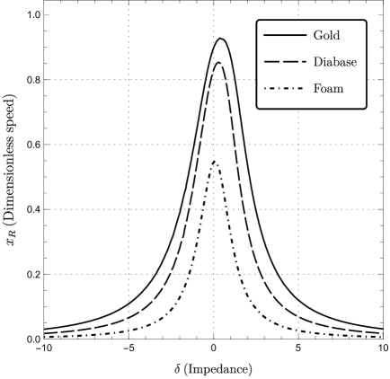
Now, we proceed as in [7] and illustrate the behavior stated above for three elastic materials, namely Gold (metal), Diabase (volcanic rock) and a polymer foam structure (auxetic material). A detailed description of these materials and their characteristics can be found in the handbook by Stacey and Page [25] (for Gold and Diabase) and in [9] (for the foam structure). The role of the elastic properties of a particular material in the secular equation is given through the dimensionless parameter , which depends on the Lame’s constants. However, for the sake of simplicity, we find in terms of the Young’s modulus and the Poisson’s ratio through the usual relations (see [1])
Straightforward calculations gives
Thus, in order to illustrate the relation of the surface wave speed and the impedance for each considered material, we just need to fix the Poisson’s ratio . Table 1 shows this elastic property for each considered material. To present the results, consider an impedance varying from a minimum value to a maximum value . The dimensionless speed is calculated by solving iteratively the secular equation (4.1), using for this the Newton-Raphson algorithm with a starting point for the iterations located at the region . The results are presented in Fig. 1. In general, the behavior can be stated as: The surface wave velocity decreases to zero as the impedance goes to and attains a maximum value at some positive impedance value .
6. Discussion
In this work we investigated the existence of surface waves in an isotropic elastic half-space endowed with a uniparametric family of impedance boundary conditions with both non-zero tangential and normal impedance. The existence and uniqueness of the surface wave for each value of the impedance parameter was demonstrated by means of the mathematical analysis of the secular equation. This has the form of the stress-free secular equation plus two additional terms regarding the impedance. The speed of the surface wave decreases asymptotically to zero for large negative and positive values of the impedance, with a maximum value for some positive value of the impedance. The theoretical findings are verified by presenting numerical results for three elastic media.
Acknowledgements
This work was supported by the National Science and Technology Council (CONACyT) of México under grant CF-2019 No. 304005.
References
- Achenbach [1975] J. Achenbach. Wave Propagation in Elastic Solids. North-Holland Series in Applied Mathematics and Mechanics. Elsevier, Amsterdam, 1975. doi: https://doi.org/10.1016/B978-0-7204-0325-1.50004-7. URL https://doi.org/10.1016/B978-0-7204-0325-1.50004-7.
- Antipov [2002] Y. A. Antipov. Diffraction of a plane wave by a circular cone with an impedance boundary condition. SIAM Journal on Applied Mathematics, 62(4):1122–1152, 2002. doi: 10.1137/S0036139900363324. URL https://doi.org/10.1137/S0036139900363324.
- Barnett et al. [1985] D. M. Barnett, J. Lothe, and P. Chadwick. Free surface (Rayleigh) waves in anisotropic elastic half-spaces: the surface impedance method. Proceedings of the Royal Society of London. A. Mathematical and Physical Sciences, 402(1822):135–152, 1985. doi: 10.1098/rspa.1985.0111. URL https://doi.org/10.1098/rspa.1985.0111.
- Bövik [1996] P. Bövik. A Comparison Between the Tiersten Model and O(H) Boundary Conditions for Elastic Surface Waves Guided by Thin Layers. Journal of Applied Mechanics, 63(1):162–167, 03 1996. ISSN 0021-8936. doi: 10.1115/1.2787193. URL https://doi.org/10.1115/1.2787193.
- Dai et al. [2010] H.-H. Dai, J. Kaplunov, and D. A. Prikazchikov. A long-wave model for the surface elastic wave in a coated half-space. Proceedings of the Royal Society A: Mathematical, Physical and Engineering Sciences, 466(2122):3097–3116, 2010. doi: 10.1098/rspa.2010.0125. URL https://doi.org/10.1098/rspa.2010.0125.
- de Lange and Raab [2013] O. L. de Lange and R. E. Raab. Electromagnetic boundary conditions in multipole theory. Journal of Mathematical Physics, 54(9), 09 2013. ISSN 0022-2488. doi: 10.1063/1.4821642. URL https://doi.org/10.1063/1.4821642. 093513.
- Godoy et al. [2012] E. Godoy, M. Durán, and J.-C. Nédélec. On the existence of surface waves in an elastic half-space with impedance boundary conditions. Wave Motion, 49(6):585–594, 2012. ISSN 0165-2125. doi: https://doi.org/10.1016/j.wavemoti.2012.03.005. URL https://doi.org/10.1016/j.wavemoti.2012.03.005.
- Hayes and Rivlin [1962] M. Hayes and R. Rivlin. A note on the secular equation for Rayleigh waves. Zeitschrift Fur Angewandte Mathematik Und Physik - ZAMP, 13:80–83, 07 1962. doi: 10.1007/BF01600759. URL http://dx.doi.org/10.1007/BF01600759.
- Lakes [1987] R. Lakes. Foam structures with a negative poisson’s ratio. Science, 235(4792):1038–1040, 1987. doi: 10.1126/science.235.4792.1038. URL https://www.science.org/doi/abs/10.1126/science.235.4792.1038.
- Li [2006] X.-F. Li. On approximate analytic expressions for the velocity of rayleigh waves. Wave Motion, 44(2):120–127, 2006. ISSN 0165-2125. doi: https://doi.org/10.1016/j.wavemoti.2006.07.003. URL https://doi.org/10.1016/j.wavemoti.2006.07.003.
- Lothe and Barnett [1976] J. Lothe and D. M. Barnett. On the existence of surface-wave solutions for anisotropic elastic half-spaces with free surface. Journal of Applied Physics, 47(2):428–433, 1976. doi: 10.1063/1.322665. URL https://doi.org/10.1063/1.322665.
- Mal et al. [2007] A. Mal, S. Banerjee, and F. Ricci. An automated damage identification technique based on vibration and wave propagation data. Philosophical Transactions of the Royal Society A: Mathematical, Physical and Engineering Sciences, 365(1851):479–491, 2007. doi: 10.1098/rsta.2006.1933. URL https://doi.org/10.1098/rsta.2006.1933.
- Malischewsky [1987] P. Malischewsky. Surface waves and discontinuities. 1 1987. URL https://www.osti.gov/biblio/6948756.
- Malischewsky [2000] P. G. Malischewsky. Comment to “A new formula for the velocity of Rayleigh waves” by D. Nkemzi [Wave Motion 26 (1997) 199–205]. Wave Motion, 31(1):93–96, 2000. ISSN 0165-2125. doi: https://doi.org/10.1016/S0165-2125(99)00025-6. URL https://doi.org/10.1016/S0165-2125(99)00025-6.
- Malischewsky Auning [2004] P. G. Malischewsky Auning. A note on Rayleigh-wave velocities as a function of the material parameters. Geofísica Internacional, 2004. ISSN 0016-7169. URL https://www.redalyc.org/articulo.oa?id=56843314.
- Martini et al. [2015] E. Martini, M. Mencagli, and S. Maci. Metasurface transformation for surface wave control. Philosophical Transactions of the Royal Society A: Mathematical, Physical and Engineering Sciences, 373(2049):20140355, 2015. doi: 10.1098/rsta.2014.0355. URL https://doi.org/10.1098/rsta.2014.0355.
- Nakamura [1991] G. Nakamura. Existence and propagation of Rayleigh waves and pulses. In J. J. Wu, T. C. T. Ting, and D. M. Barnett, editors, Modern Theory of Anisotropic Elasticity and Applications, pages 215–231. Society for Industrial and Applied Mathematics, Philadelphia, PA, 1991. URL https://books.google.com.mx/books?id=2fwUdSTN_6gC. Proceedings of the Workshop on Anisotropic Elasticity and its Applications (Research Triangle Park, NC, 1990).
- Pham and Vinh [2021] H. G. Pham and P. Vinh. Existence and uniqueness of Rayleigh waves with normal impedance boundary conditions and formula for the wave velocity. Journal of Engineering Mathematics, 130:13, 10 2021. doi: 10.1007/s10665-021-10170-y. URL https://doi.org/10.1007/s10665-021-10170-y.
- Qin and Colton [2012] H. H. Qin and D. Colton. The inverse scattering problem for cavities with impedance boundary condition. Advances in Computational Mathematics, 36:157–174, 2012. URL https://doi.org/10.1007/s10444-011-9179-2.
- Rahman and Barber [1995] M. Rahman and J. R. Barber. Exact Expressions for the Roots of the Secular Equation for Rayleigh Waves. Journal of Applied Mechanics, 62(1):250–252, 03 1995. ISSN 0021-8936. doi: 10.1115/1.2895917. URL https://doi.org/10.1115/1.2895917.
- Rahman and Michelitsch [2006] M. Rahman and T. Michelitsch. A note on the formula for the Rayleigh wave speed. Wave Motion, 43(3):272–276, 2006. ISSN 0165-2125. doi: https://doi.org/10.1016/j.wavemoti.2005.10.002. URL https://doi.org/10.1016/j.wavemoti.2005.10.002.
- Rayleigh [1885] L. Rayleigh. On waves propagating along the plane surface of an elastic solid. Proceedings of the London Mathematical Society, s1-17(1):4–11, 1885. doi: https://doi.org/10.1112/plms/s1-17.1.4. URL https://doi.org/10.1112/plms/s1-17.1.4.
- Ru [2023] C. Ru. Rayleigh waves in an elastic half-space with a hard sphere-filled metasurface. Mechanics Research Communications, 131:104148, 2023. ISSN 0093-6413. doi: 10.1016/j.mechrescom.2023.104148. URL https://doi.org/10.1016/j.mechrescom.2023.104148.
- Senior [1960] T. Senior. Impedance boundary conditions for imperfectly conducting surfaces. Applied Scientific Research, Sect B, 8(4):418–436, 1960. doi: 10.1007/BF02920074. URL https://doi.org/10.1007/BF02920074.
- Stacey and Page [1986] T. Stacey and C. Page. Practical Handbook for Underground Rock Mechanics. Series on rock and soil mechanics. Trans Tech, 1986. ISBN 9780878490561. URL https://books.google.com.mx/books?id=u-5OAQAAIAAJ.
- Stupfel and Poget [2011] B. Stupfel and D. Poget. Sufficient uniqueness conditions for the solution of the time harmonic maxwell’s equations associated with surface impedance boundary conditions. Journal of Computational Physics, 230(12):4571–4587, 2011. ISSN 0021-9991. doi: https://doi.org/10.1016/j.jcp.2011.02.032. URL https://doi.org/10.1016/j.jcp.2011.02.032.
- Tiersten [1969] H. F. Tiersten. Elastic surface waves guided by thin films. Journal of Applied Physics, 40(2):770–789, 1969. doi: 10.1063/1.1657463. URL https://doi.org/10.1063/1.1657463.
- Ting [2002] T. C. T. Ting. An Explicit Secular Equation for Surface Waves in an Elastic Material of General Anisotropy. The Quarterly Journal of Mechanics and Applied Mathematics, 55(2):297–311, 05 2002. ISSN 0033-5614. doi: 10.1093/qjmam/55.2.297. URL https://doi.org/10.1093/qjmam/55.2.297.
- Ting [2005] T. C. T. Ting. Explicit secular equations for surface waves in an anisotropic elastic half-space from rayleigh to today. In R. V. Goldstein and G. A. Maugin, editors, Surface Waves in Anisotropic and Laminated Bodies and Defects Detection, pages 95–116, Dordrecht, 2005. Springer Netherlands. ISBN 978-1-4020-2387-3. URL https://doi.org/10.1007/1-4020-2387-1_4.
- Vallejo [2024] F. Vallejo. The secular equation for elastic surface waves under non standard boundary conditions of impedance type: A perspective from linear algebra. 2024. doi: https://doi.org/10.48550/arXiv.2308.12407. URL https://doi.org/10.48550/arXiv.2308.12407.
- Vinh and Linh [2012] P. C. Vinh and N. T. K. Linh. An approximate secular equation of Rayleigh waves propagating in an orthotropic elastic half-space coated by a thin orthotropic elastic layer. Wave Motion, 49(7):681–689, 2012. ISSN 0165-2125. doi: https://doi.org/10.1016/j.wavemoti.2012.04.005. URL https://doi.org/10.1016/j.wavemoti.2012.04.005.
- Vinh and Ngoc Anh [2014] P. C. Vinh and V. T. Ngoc Anh. Rayleigh waves in an orthotropic half-space coated by a thin orthotropic layer with sliding contact. International Journal of Engineering Science, 75:154–164, 2014. ISSN 0020-7225. doi: https://doi.org/10.1016/j.ijengsci.2013.11.004. URL https://doi.org/10.1016/j.ijengsci.2013.11.004.
- Vinh and Ogden [2004a] P. C. Vinh and R. Ogden. Formulas for the Rayleigh wave speed in orthotropic elastic solids. Archives of Mechanics, 56(3):247–265, 2004a. URL https://am.ippt.pan.pl/am/article/view/161/0.
- Vinh and Ogden [2004b] P. C. Vinh and R. Ogden. On formulas for the Rayleigh wave speed. Wave Motion, 39(3):191–197, 2004b. ISSN 0165-2125. doi: https://doi.org/10.1016/j.wavemoti.2003.08.004. URL https://doi.org/10.1016/j.wavemoti.2003.08.004.
- Vinh and Xuan [2017] P. C. Vinh and N. Q. Xuan. Rayleigh waves with impedance boundary condition: Formula for the velocity, existence and uniqueness. European Journal of Mechanics - A/Solids, 61:180–185, 2017. ISSN 0997-7538. doi: https://doi.org/10.1016/j.euromechsol.2016.09.011. URL https://doi.org/10.1016/j.euromechsol.2016.09.011.
- Ylä‐Oijala and Järvenpää [2006] P. Ylä‐Oijala and S. Järvenpää. Iterative solution of high-order boundary element method for acoustic impedance boundary value problems. Journal of Sound and Vibration, 291(3):824–843, 2006. ISSN 0022-460X. doi: https://doi.org/10.1016/j.jsv.2005.06.044. URL https://doi.org/10.1016/j.jsv.2005.06.044.
- Zakharov [2006] D. Zakharov. Surface and internal waves in a stratified layer of liquid and an analysis of the impedance boundary conditions. Journal of Applied Mathematics and Mechanics, 70(4):573–581, 2006. ISSN 0021-8928. doi: https://doi.org/10.1016/j.jappmathmech.2006.09.008. URL https://doi.org/10.1016/j.jappmathmech.2006.09.008.