EnCoMP: Enhanced Covert Maneuver Planning using Offline Reinforcement Learning

Abstract

Cover navigation in complex environments is a critical challenge for autonomous robots, requiring the identification and utilization of environmental cover while maintaining efficient navigation. We propose an enhanced navigation system that enables robots to identify and utilize natural and artificial environmental features as cover, thereby minimizing exposure to potential threats. Our perception pipeline leverages LiDAR data to generate high-fidelity cover maps and potential threat maps, providing a comprehensive understanding of the surrounding environment. We train an offline reinforcement learning model using a diverse dataset collected from real-world environments, learning a robust policy that evaluates the quality of candidate actions based on their ability to maximize cover utilization, minimize exposure to threats, and reach the goal efficiently. Extensive real-world experiments demonstrate the superiority of our approach in terms of success rate, cover utilization, exposure minimization, and navigation efficiency compared to state-of-the-art methods.

1 Introduction

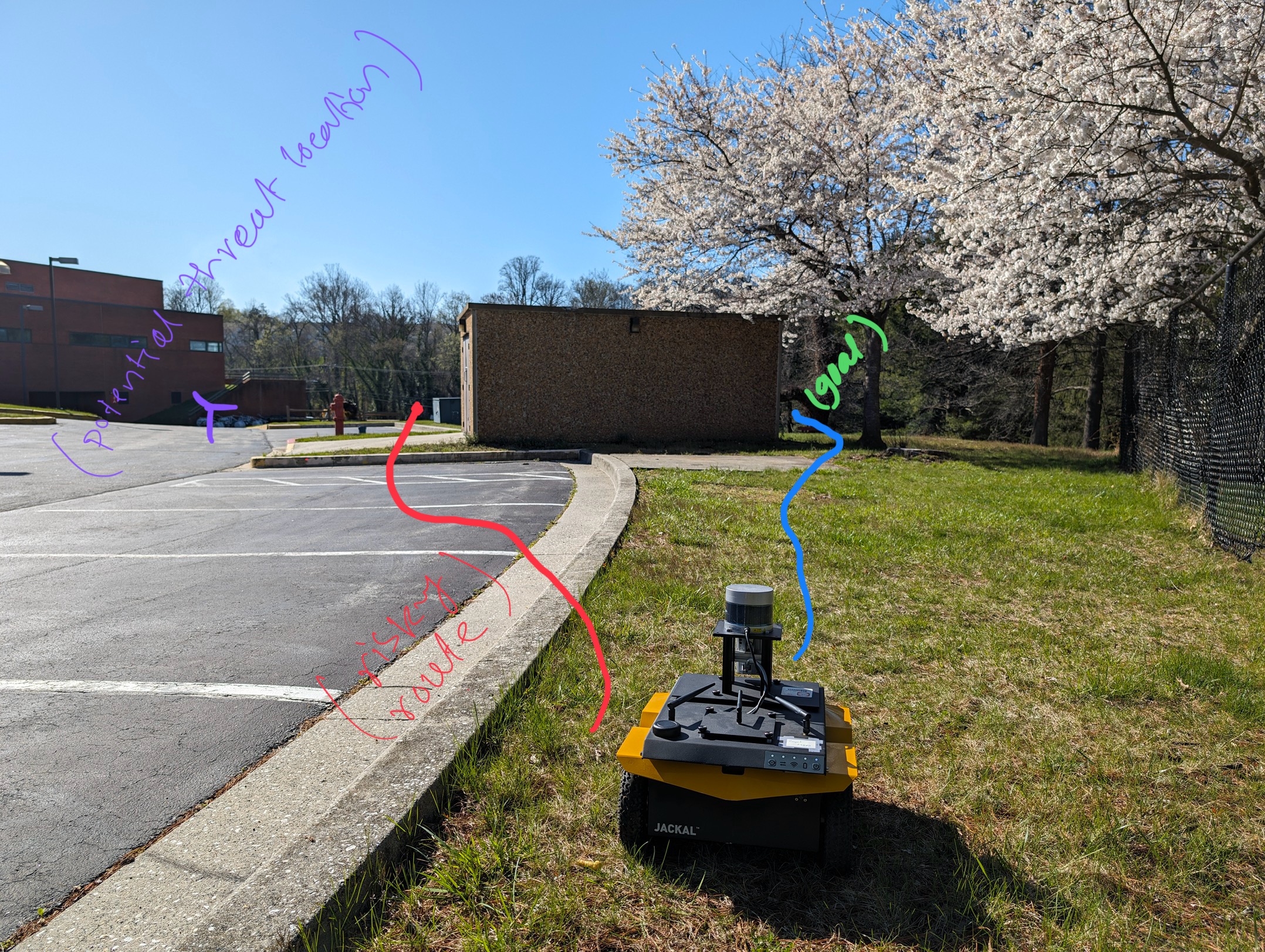
Figure 1: EnCoMP Covert Navigation Strategies: In this outdoor environment, the robot (Jackal) is navigating towards a goal location. To reach the goal while avoiding potential threats (purple marked), it identifies and moves towards nearby trees and a small brick building structure that can provide cover and concealment. By utilizing the natural obstacles in the environment strategically, the robot aims to minimize its visibility and exposure as it traverses the open field to reach its destination safely.

.

Autonomous navigation in complex environments is a critical capability for robots operating in various applications, such as military reconnaissance ‘[33], search and rescue missions  [2], and surveillance operations  [38]. These scenarios pose unique challenges for robots, requiring them to accurately perceive the environment, identify potential cover, and adapt their navigation strategies to minimize exposure to threats while efficiently reaching the goal. Existing approaches to covert navigation often rely on pre-defined environmental models  [15, 27] or supervised learning techniques  [4, 23] that require extensive manual annotation and labeling of traversable terrain. However, these methods may not align with the actual traversability capabilities of different robots due to varying dynamic constraints, leading to conservative and inefficient navigation behaviors  [8, 9].

Reinforcement learning (RL) is a promising approach for autonomous navigation, enabling robots to learn complex strategies through interaction with the environment [19, 26]. Online RL methods have been applied to outdoor navigation [13, 32], eliminating the need for human labeling. However, these methods often suffer from severe performance degradation during real-world deployment due to sim-to-real transfer issues  [35, 3]. Training complex models using online RL requires high-fidelity simulations, which may not be available for intricate environments. Offline RL  [17, 12] has been proposed to mitigate these limitations by training models using data collected in real-world environments, reducing sim-to-real transfer problems. Despite the advancements in RL-based navigation, existing methods have not fully exploited the rich information provided by modern sensors, such as LiDAR, which can offer valuable insights into the environment’s properties and potential cover  [39, 18].

To address these challenges, we propose an enhanced covert navigation framework that leverages LiDAR data, height maps, cover maps, potential threat maps, and offline reinforcement learning. Our approach enables robots to identify and utilize natural and artificial environmental features as cover, thereby minimizing exposure to potential threats while maintaining efficient navigation.

The main contributions of this work are as follows:

1. Novel Integration of LiDAR Data for Covert Navigation: We present EnCoMP, an innovative framework that uniquely combines LiDAR data, not just for mapping but explicitly for enhancing covert navigation. Unlike previous works that primarily focus on the navigational aspects, Multi-Map Generation utilizes LiDAR to perceive environmental features that offer potential cover, optimizing the robot’s path for minimal exposure.

2. Advanced Multi-Modal Perception Pipeline: Our system introduces a cutting-edge perception pipeline that fuses LiDAR-derived height and cover density maps. This approach surpasses traditional single-modality perception in understanding complex environments, enabling more informed navigation decisions under covert operation scenarios.

The remainder of this paper is organized as follows: Section 2 provides an overview of related work in covert navigation. Some related background information is present in Section 3 Section 4 presents our proposed covert navigation framework, detailing the multi-modal perception pipeline, offline reinforcement learning algorithm, and policy transfer to a physical robot platform. Section 6 describes the experimental setup and presents the results of our real-world tests. Finally, Section 7 concludes the paper and discusses potential future research directions.

2 Related Work

2.1 Perception for Outdoor Navigation

Accurate perception of the environment is crucial for autonomous navigation in complex outdoor scenes. Traditional approaches rely on supervised learning techniques, such as semantic segmentation [30] and object detection [29], to identify traversable terrain and potential cover. However, these methods require extensive manual annotation and may not generalize well to novel environments or robot platforms [25, 36]. Recent works have explored self-supervised learning [30] and adversarial training [6] to reduce the reliance on human annotation. While these techniques have shown promise, they still struggle to fully capture the complex properties and dynamics of real-world environments.

In contrast to these approaches, our framework leverages multi-modal sensory information, specifically LiDAR intensity and height data, to generate high-fidelity cover maps and potential threat maps. This allows the robot to accurately perceive and reason about the environment’s properties and potential cover without relying on extensive manual annotation.

2.2 Offline Reinforcement Learning for Navigation

Offline reinforcement learning is a promising approach for learning navigation policies from previously collected datasets, mitigating the challenges associated with online learning in real-world environments [16, 7]. Recent works have demonstrated the effectiveness of offline reinforcement learning for navigation tasks in simulated environments [20, 10]. Mandlekar et al. [20] proposed IRIS, an offline reinforcement learning framework for robotic manipulation tasks. Their approach learns a policy from a dataset of human demonstrations and achieves competitive performance compared to online learning methods. Similarly, Hansen et al. [10] introduced a generalization through offline reinforcement learning framework that learns a navigation policy from a diverse dataset of trajectories in simulated environments.

Our approach builds upon these advancements by introducing an offline reinforcement learning framework specifically designed for covert navigation in complex outdoor environments. By learning from a diverse dataset collected from real-world settings, our approach can effectively capture the complex dynamics and uncertainties present in these environments and generate robust navigation strategies.

2.3 Covert Navigation

Covert navigation is a critical capability for robots operating in hostile or sensitive environments, where the primary objective is to reach a designated goal while minimizing the risk of detection by potential threats [1, 24]. Existing approaches to stealth navigation often rely on heuristic methods [34] or potential field-based techniques [21] to identify potential cover and minimize exposure. However, these methods may not effectively capture the complex dynamics and uncertainties present in real-world environments. Recent works have explored the use of reinforcement learning for stealth navigation  [22]. While these approaches have shown promise in learning adaptive strategies, they often rely on simplified environmental representations and do not fully exploit the rich sensory information available in real-world settings.

Our framework addresses these limitations by integrating multi-modal perception and offline reinforcement learning to enable robots to navigate covertly and efficiently in complex outdoor environments. By learning from a diverse dataset of real-world experiences, our approach can effectively capture the complex dynamics and uncertainties present in these settings and generate robust navigation strategies.

3 Background

3.1 Problem Formulation

We formulate the covert navigation problem as a Markov Decision Process (MDP) defined by the tuple $(\mathcal{S},\mathcal{A},\mathcal{P},\mathcal{R},\gamma)$, where $\mathcal{S}$ is the state space, $\mathcal{A}$ is the action space, $\mathcal{P}$ is the transition probability function, $\mathcal{R}$ is the reward function, and $\gamma$ is the discount factor. The state space $\mathcal{S}$ includes the robot’s position $\mathbf{s}_{r}\in\mathbb{R}^{2}$, the goal position $\mathbf{s}_{g}\in\mathbb{R}^{2}$, the height map $\mathbf{H}\in\mathbb{R}^{M\times N}$, the cover map $\mathbf{C}\in\mathbb{R}^{M\times N}$, and the threat map $\mathbf{T}\in\mathbb{R}^{M\times N}$, where $M$ and $N$ are the dimensions of the maps. The height map represents the elevation of the terrain, the cover map indicates the presence and quality of cover objects, and the threat map represents the estimated positions and line-of-sight of potential threats in the environment. The action space $\mathcal{A}$ consists of the robot’s navigation actions, such as moving forward, turning left, turning right, or staying in place. The transition probability function $\mathcal{P}(s^{\prime}\mid s,a)$ defines the probability of transitioning from state $s$ to state $s^{\prime}$ when taking action $a$. The reward function $\mathcal{R}(s,a)$ assigns a scalar value to each state-action pair, taking into account the robot’s distance to the goal, the level of cover utilized, and the exposure to potential threats. The reward function is designed to encourage the robot to reach the goal efficiently while maximizing the use of cover and minimizing the risk of being detected by threats. The discount factor $\gamma\in[0,1]$ determines the importance of future rewards compared to immediate rewards. The objective is to learn an optimal policy $\pi^{*}:\mathcal{S}\rightarrow\mathcal{A}$ that maximizes the expected cumulative discounted reward:

$$\pi^{*}=\arg\max_{\pi}\mathbb{E}_{\pi}\left[\sum_{t=0}^{\infty}\gamma^{t}r_{t}\right]$$ (1)

where $r_{t}$ is the reward received at time step $t$.

3.2 Offline Reinforcement Learning

In the context of our covert navigation problem, we face the challenge of learning an effective policy from a fixed dataset without further interaction with the environment. While offline reinforcement learning offers a promising approach, directly applying standard reinforcement learning algorithms to offline datasets can lead to suboptimal performance. This is due to several factors, such as the mismatch between the distribution of states and actions in the dataset and the distribution induced by the learned policy, as well as the potential for overestimation of Q-values for unseen state-action pairs [28].

To address these challenges, we employ the Conservative Q-Learning (CQL) algorithm [14] as our offline reinforcement learning method. CQL is an off-policy algorithm that aims to learn a conservative estimate of the Q-function by incorporating a regularization term in the training objective. The key idea behind CQL is to encourage the learned Q-function to assign lower values to unseen or out-of-distribution actions while still accurately fitting the Q-values for actions observed in the dataset. The CQL algorithm modifies the standard Q-learning objective by adding a regularization term that penalizes overestimation of Q-values. This regularization term is based on the difference between the expected Q-value under the learned policy and the expected Q-value under the behavior policy used to collect the dataset. By minimizing this difference, CQL encourages the learned Q-function to be conservative in its estimates, especially for state-action pairs that are not well-represented in the dataset.

4 EnCoMP: Enhanced Covert Maneuver Planning

In this section, We explain the major stages of the EnCoMP approach. Fig. 2 shows how different modules in our method are connected.

5 Dataset Generation

Our raw training data is collected by navigating a ground robot equipped with a 3D LiDAR sensor through various outdoor environments for approximately 6 hours. The robot is teleoperated to explore diverse terrains, including open fields, wooded areas, and urban settings with a mix of natural and artificial cover objects. During data collection, we record raw 3D point clouds, the robot’s odometry, and GPS coordinates at each time step.

To create a goal-conditioned dataset $\mathcal{D}$ with a series of $\{\mathbf{s}_{j},\mathbf{a}_{j},r_{j},\mathbf{s}^{\prime}_{j}\}$, we first process the raw point cloud data to generate height maps $\mathcal{H}$, cover maps $\mathcal{C}$, and threat maps $\mathcal{T}$ for each time step. The height map $\mathcal{H}$ represents the elevation of the terrain, the cover map $\mathcal{C}$ indicates the presence and quality of cover objects, and the threat map $\mathcal{T}$ represents the estimated positions and line-of-sight of potential threats in the environment. Next, we sample random trajectory segments from the processed dataset. For each segment, we select a random initial state $\mathbf{s}_{j}$ and a future state $\mathbf{s}^{\prime}_{j}$ as the goal state, ensuring that the goal state is within a reasonable distance (e.g., 10-30 meters) from the initial state. The action $\mathbf{a}_{j}$ is derived from the robot’s odometry and represents the motion command executed to transition from state $\mathbf{s}_{j}$ to the next state in the original trajectory. To introduce diversity in the goal locations and threat distributions, we augment the dataset by applying random rotations and translations to the height maps $\mathcal{H}$, cover maps $\mathcal{C}$, and threat maps $\mathcal{T}$. This augmentation helps to improve the generalization capability of the learning algorithm. The final processed dataset $\mathcal{D}=\{(\mathbf{s}_{j},\mathbf{a}_{j},r_{j},\mathbf{s}^{\prime}_{j})\mid j=1,2,\ldots,N\}$ consists of $N$ goal-conditioned trajectories, where each trajectory is represented by a sequence of state-action-reward-next_state tuples. The state $\mathbf{s}_{j}$ includes the height map $\mathcal{H}_{j}$, cover map $\mathcal{C}_{j}$, threat map $\mathcal{T}_{j}$, and the robot’s position $\mathbf{p}_{j}$ at time step $j$. The next state $\mathbf{s}^{\prime}_{j}$ represents the state reached after executing action $\mathbf{a}_{j}$ in state $\mathbf{s}_{j}$. This processed dataset is then used to train the covert navigation policy using offline reinforcement learning. The policy learns to generate actions that maximize the expected cumulative reward, taking into account the terrain height, cover availability, and threat exposure.

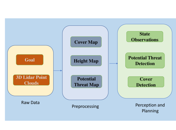
Figure 2: Overview of EnCoMP System Architecture.

5.1 Finding Cover in the Environment

To identify cover objects in the environment, we process the LiDAR point cloud $\mathcal{P}=\{\mathbf{p}_{i}\in\mathbb{R}^{3}\mid i=1,\dots,N\}$, where each point $\mathbf{p}_{i}$ is represented by its 3D coordinates $(x_{i},y_{i},z_{i})$. We apply the following steps:

Point Cloud Segmentation: We use the Euclidean cluster extraction algorithm to segment the point cloud into distinct objects. The algorithm groups nearby points based on their Euclidean distance, forming clusters $\mathcal{C}_{j}\subset\mathcal{P}$, where $j=1,\dots,M$ and $M$ is the number of clusters.

Cover Object Identification: For each cluster $\mathcal{C}_{j}$, we calculate its height $h_{j}$, density $d_{j}$, and volume $v_{j}$ as follows:

$$h_{j} =\max_{\mathbf{p}_{i}\in\mathcal{C}_{j}}z_{i}-\min_{\mathbf{p}_{i}\in\mathcal{C}_{j}}z_{i},$$ (2)

$$d_{j} =\frac{|\mathcal{C}_{j}|}{v_{j}},$$ (3)

$$v_{j} =(x_{j,\max}-x_{j,\min})\times(y_{j,\max}-y_{j,\min})\times h_{j},$$ (4)

where $|\mathcal{C}_{j}|$ is the number of points in cluster $\mathcal{C}_{j}$, and $x_{j,\min},x_{j,\max},y_{j,\min},y_{j,\max}$ are the minimum and maximum coordinates of the cluster in the $x$ and $y$ dimensions, respectively. A cluster $\mathcal{C}_{j}$ is considered a cover object if it satisfies the following criteria:

$$h_{j} \geq h_{\min},$$ (5)

$$d_{j} \geq d_{\min},$$ (6)

$$v_{j} \geq v_{\min},$$ (7)

where $h_{\min},d_{\min},v_{\min}$ are predefined thresholds for height, density, and volume, respectively.

5.2 Generating Cover Maps

The cover map $\mathcal{M}_{c}$ is a 2D grid representation of the environment, where each cell $(i,j)$ contains the cover density value $c_{i,j}\in[0,1]$. We generate the cover map using the identified cover objects as follows:

1. Initialize the cover map $\mathcal{M}_{c}$ with dimensions $H\times W$ and cell size $\delta$.

2. For each cover object $\mathcal{C}_{j}$, project its points onto the corresponding cells in the cover map. The projection of a point $\mathbf{p}_{i}=(x_{i},y_{i},z_{i})$ to a cell $(i,j)$ is given by:

   $$i =\left\lfloor\frac{x_{i}-x_{\min}}{\delta}\right\rfloor,$$ (8)

   $$j =\left\lfloor\frac{y_{i}-y_{\min}}{\delta}\right\rfloor,$$ (9)

   where $x_{\min},y_{\min}$ are the minimum coordinates of the environment in the $x$ and $y$ dimensions, respectively.

3. For each cell $(i,j)$ in the cover map, calculate the cover density $c_{i,j}$ as:

   $$c_{i,j}=\frac{|\mathcal{P}_{i,j}^{c}|}{|\mathcal{P}_{i,j}|},$$ (10)

   where $\mathcal{P}_{i,j}$ is the set of all LiDAR points projected onto cell $(i,j)$, and $\mathcal{P}_{i,j}^{c}\subseteq\mathcal{P}_{i,j}$ is the subset of points belonging to cover objects.

5.3 Generating Potential Threat Maps

The potential threat map $\mathcal{M}_{t}$ is a 2D grid representation of the environment, where each cell $(i,j)$ contains the potential threat level $t_{i,j}\in[0,1]$. We generate the potential threat map using the following steps:

1. Initialize the potential threat map $\mathcal{M}_{t}$ with the same dimensions and cell size as the cover map.

2. Randomly place $K$ potential threats in the environment at locations $\mathbf{t}_{k}=(x_{k},y_{k}),k=1,\dots,K$.

3. For each cell $(i,j)$ in the potential threat map, calculate the potential threat level $t_{i,j}$ as:

   $$t_{i,j}=\max_{k=1}^{K}\left(\frac{1}{d_{i,j,k}}\right)\cdot\mathbbm{1}[\text{LOS}(\mathbf{p}_{i,j},\mathbf{t}_{k})],$$ (11)

   where $d_{i,j,k}$ is the Euclidean distance between the center of cell $(i,j)$, denoted as $\mathbf{p}_{i,j}$, and the $k$-th potential threat location $\mathbf{t}_{k}$. $\mathbbm{1}[\text{LOS}(\mathbf{p}_{i,j},\mathbf{t}_{k})]$ is an indicator function that equals 1 if there is a line of sight between $\mathbf{p}_{i,j}$ and $\mathbf{t}_{k}$, and 0 otherwise. The line of sight is determined using Bresenham’s ray tracing algorithm [5].

5.4 Generating Height Maps

The height map $\mathcal{M}_{h}$ is a 2D grid representation of the environment, where each cell $(i,j)$ contains the maximum height value $h_{i,j}\in\mathbb{R}$. We generate the height map using the LiDAR point cloud as follows:

1. Initialize the height map $\mathcal{M}_{h}$ with the same dimensions and cell size as the cover map.

2. For each LiDAR point $\mathbf{p}_{i}=(x_{i},y_{i},z_{i})$, project it onto the corresponding cell $(i,j)$ in the height map using the projection equations defined earlier.

3. For each cell $(i,j)$ in the height map, calculate the maximum height value $h_{i,j}$ as:

   $$h_{i,j}=\max_{\mathbf{p}_{i}\in\mathcal{P}_{i,j}}z_{i},$$ (12)

   where $\mathcal{P}_{i,j}$ is the set of all LiDAR points projected onto cell $(i,j)$.

5.5 Reward Functions

We design the following reward functions to capture the objectives of the covert navigation problem:

5.5.1 Cover Utilization Reward

The cover utilization reward encourages the robot to navigate through areas with high cover density, as indicated by the cover map $\mathcal{C}$. It is defined as:

$$R_{\text{cover}}(s,a)=\lambda_{c}\sum_{i=1}^{M}\sum_{j=1}^{N}\mathcal{C}_{ij}\cdot\mathbbm{1}\left[(x_{i},y_{j})\in\xi(s,a)\right]$$ (13)

where $\lambda_{c}$ is a positive weighting factor, $\mathcal{C}_{ij}$ is the cover density value at cell $(i,j)$ in the cover map, $\mathbbm{1}[\cdot]$ is the indicator function, and $\xi(s,a)$ is the set of cells traversed by the robot when taking action $a$ in state $s$.

5.5.2 Threat Exposure Penalty

The threat exposure penalty discourages the robot from being exposed to potential threats, as indicated by the potential threat map $\mathcal{T}$. It is defined as:

$$R_{threat}(s)=-\lambda_{t}\sum_{i=1}^{M}\sum_{j=1}^{N}\mathcal{T}_{ij}\cdot\mathbbm{1}[(x_{i},y_{j})\in\xi(s)]$$ (14)

where $\lambda_{t}$ is a positive weighting factor, $\mathcal{T}_{ij}$ is the threat level at cell $(i,j)$ in the potential threat map, and $\xi(s)$ is the set of cells occupied by the robot in state $s$.

5.5.3 Goal Reaching Reward

The goal reaching reward encourages the robot to make progress towards the goal position. It is defined as:

$$R_{goal}(s,a)=\lambda_{g}(d(s,g)-d(s^{\prime},g))$$ (15)

where $\lambda_{g}$ is a positive weighting factor, $d(s,g)$ is the distance between the robot’s position in state $s$ and the goal position $g$, and $s^{\prime}$ is the state reached after taking action $a$ in state $s$.

5.5.4 Collision Avoidance Penalty

The collision avoidance penalty discourages the robot from colliding with obstacles or navigating through untraversable regions, as indicated by the height map $\mathcal{H}$. It is defined as:

$$R_{\text{collision}}(s,a)=\begin{cases}-\lambda_{o},&\text{if }\exists(x_{i},y_{j})\in\xi(s,a),\mathcal{H}_{ij}>h_{\max},\\ 0,&\text{otherwise.}\end{cases}$$ (16)

where $\lambda_{o}$ is a large positive constant, $\mathcal{H}_{ij}$ is the height value at cell $(i,j)$ in the height map, and $h_{max}$ is the maximum traversable height threshold.

5.6 CQL Policy Learning with Multi-modal Map Inputs

We employ Conservative Q-Learning (CQL) to learn the covert navigation policy from the diverse dataset $\mathcal{D}$ collected from real-world environments. CQL learns a conservative estimate of the Q-function by incorporating a regularization term in the training objective, which encourages the learned Q-function to assign lower values to out-of-distribution actions while still accurately fitting the Q-values for actions observed in the dataset. The CQL objective is defined as:

$$\begin{split}\mathcal{L}(\theta)=\mathbb{E}_{(\mathbf{s},\mathbf{a},r,\mathbf{s}^{\prime})\sim\mathcal{D}}\Big{[}&(Q_{\theta}(\mathbf{s},\mathbf{a})-\\ &(r+\gamma\mathbb{E}_{\mathbf{a}^{\prime}\sim\pi_{\theta}(\cdot\mid\mathbf{s}^{\prime})}[Q_{\theta}(\mathbf{s}^{\prime},\mathbf{a}^{\prime})]))^{2}\Big{]}\\ &+\alpha\mathcal{R}(\theta)\end{split}$$ (17)

where $Q_{\theta}$ is the Q-function parameterized by $\theta$, $\pi_{\theta}$ is the policy, $\alpha$ is a hyperparameter controlling the strength of the regularization term $\mathcal{R}(\theta)$, and $\mathcal{D}$ is the dataset of transitions.

The regularization term $\mathcal{R}(\theta)$ is defined as:

$$\begin{split}\mathcal{R}(\theta)=\mathbb{E}_{\mathbf{s}\sim\mathcal{D}}\bigg{[}&\log\sum_{\mathbf{a}}\exp(Q_{\theta}(\mathbf{s},\mathbf{a}))\\ &-\mathbb{E}_{\mathbf{a}\sim\pi_{\beta}(\cdot\mid\mathbf{s})}[Q_{\theta}(\mathbf{s},\mathbf{a})]\bigg{]}\end{split}$$ (18)

where $\pi_{\beta}$ is the behavior policy used to collect the dataset $\mathcal{D}$. To learn the covert navigation policy, we use the high-fidelity cover map $\mathcal{C}$, potential threat map $\mathcal{T}$, and height map $\mathcal{H}$ as input to the Q-function and policy networks. The state input to the networks is defined as:

$$\mathbf{s}=[\mathcal{C},\mathcal{T},\mathcal{H},\mathbf{p}_{r},\mathbf{p}_{g}]$$ (19)

where $\mathbf{p}_{r}$ and $\mathbf{p}_{g}$ are the robot’s position and goal position, respectively.

During training, the CQL algorithm samples batches of transitions $(\mathbf{s},\mathbf{a},r,\mathbf{s}^{\prime})$ from the dataset $\mathcal{D}$ and updates the Q-function and policy networks using the CQL objective. The Q-function network learns to estimate the expected cumulative reward for each state-action pair, while the policy network learns to select actions that maximize the Q-values. By incorporating the multi-modal map inputs and utilizing the conservative Q-learning objective, the learned policy effectively navigates the robot towards the goal while maximizing cover utilization, minimizing threat exposure, and avoiding collisions. The CQL algorithm ensures that the learned policy is robust and generalizes well to novel environments by penalizing overestimation of Q-values for out-of-distribution actions.

During deployment, the learned policy takes the current state $\mathbf{s}$, which includes the multi-modal map inputs, and outputs the optimal action $\mathbf{a}^{*}$ to navigate the robot covertly and efficiently:

$$\mathbf{a}^{*}=\pi_{\theta}(\mathbf{s})$$ (20)

The robot executes the selected action and observes the next state $\mathbf{s}^{\prime}$ and reward $r$. This process is repeated until the robot reaches the goal or a maximum number of steps is reached.

By leveraging the multi-modal map inputs and the CQL algorithm, our approach learns a robust and efficient policy for covert navigation in complex environments, enabling the robot to make informed decisions based on the comprehensive understanding of the environment provided by the cover map, potential threat map, and height map.

6 Experiments and Results

In this section, we present the experimental setup, results, and analysis of the EnCoMP framework. We evaluate the performance of EnCoMP in both simulated and real-world environments and compare it with state-of-the-art baselines.

6.1 Evaluation Metrics

We evaluate the performance of EnCoMP and the baselines using the following metrics:

• Success Rate: The percentage of trials in which the robot successfully reaches the goal location without being detected by threats or colliding with obstacles.

• Navigation Time: The average time taken by the robot to navigate from the start position to the goal location in successful trials.

• Trajectory Length: The average length of the path traversed by the robot from the start position to the goal location in successful trials.

• Threat Exposure: The average percentage of time the robot is exposed to threats during navigation, calculated as the ratio of the time spent in the line-of-sight of threats to the total navigation time.

• Cover Utilization: The average percentage of time the robot utilizes cover objects during navigation, calculated as the ratio of the time spent in high cover density areas (as indicated by the cover map) to the total navigation time.

6.2 Baselines

We compare the performance of EnCoMP against the following state-of-the-art navigation methods:

• CoverNav: A deep reinforcement learning-based system designed for navigation planning that prioritizes the use of natural cover in unstructured outdoor environments. This strategy aims to enhance stealth and safety in potentially hostile settings. [11]

• VAPOR: A method for autonomous legged robot navigation in unstructured, densely vegetated outdoor environments using offline Reinforcement Learning (RL).[37]

• VERN: An approach for vegetation-aware robot navigation, which facilitates efficient traversal in densely vegetated and unstructured outdoor environments. Their method integrates sensory data and learning algorithms to navigate with an understanding of vegetation density and type. [31]

6.3 Implementation Details

Our offline RL network is implemented in PyTorch and trained in a workstation with a 10th-generation Intel Core i9-10850K processor and an NVIDIA GeForce RTX 3090 GPU. For real-time deployment and inference, we use the Jackal UGV from Clearpath Robotics equipped with a 3D VLP-32C Velodyne Ultrapuck LiDAR. It also includes an onboard Intel computer system, equipped with an Intel i7-9700TE CPU and an NVIDIA GeForce GTX 1650 Ti GPU.

6.4 Testing Scenarios

We evaluate our covert-based navigation framework in three diverse outdoor environments:

• Scenario 1: An urban environment with buildings, structures, and sparse vegetation.

• Scenario 2: A densely vegetated forest environment with trees, bushes, and uneven terrain.

• Scenario 3: A mixed environment with both urban structures and natural vegetation.

Each scenario presents unique challenges for covert navigation, such as varying levels of cover availability, threat exposure, and terrain complexity.

6.5 Performance Comparison and Analysis

Table 1 demonstrates EnCoMP’s significant improvements over existing navigation systems across all evaluation metrics and testing scenarios. In terms of success rate, EnCoMP consistently outperforms the baseline methods across all scenarios, achieving success rates of 95%, 93%, and 91% in Scenarios 1, 2, and 3, respectively. This demonstrates the effectiveness of our approach in navigating complex environments while maintaining covertness and avoiding threats. EnCoMP also exhibits the shortest navigation times and trajectory lengths compared to the baselines, indicating its efficiency in reaching the goal location. The reduced navigation times and trajectory lengths can be attributed to the informed decision-making enabled by the multi-modal perception pipeline and the learned covert navigation policy. Our approach achieves the highest exploration coverage percentages, demonstrating its ability to thoroughly explore the environment while navigating towards the goal. The high exploration coverage ensures that the robot can identify potential cover locations and threats more effectively.

Notably, EnCoMP significantly reduces the threat exposure percentage compared to the baselines, with values of 10.5%, 12.0%, and 14.5% in Scenarios 1, 2, and 3, respectively. This highlights the effectiveness of our approach in minimizing the robot’s visibility to threats and maintaining a high level of covertness during navigation. Furthermore, EnCoMP achieves the highest cover utilization percentages, indicating its ability to effectively leverage the available cover objects in the environment. By actively seeking and utilizing cover, our approach enhances the robot’s survivability and reduces the risk of detection.

Fig. 3 presents sample navigation trajectories generated by EnCoMP and the baseline methods in the three testing scenarios. As evident from the trajectories, EnCoMP generates paths that prioritize cover utilization and threat avoidance, while the baseline methods often result in more exposed and less efficient paths.

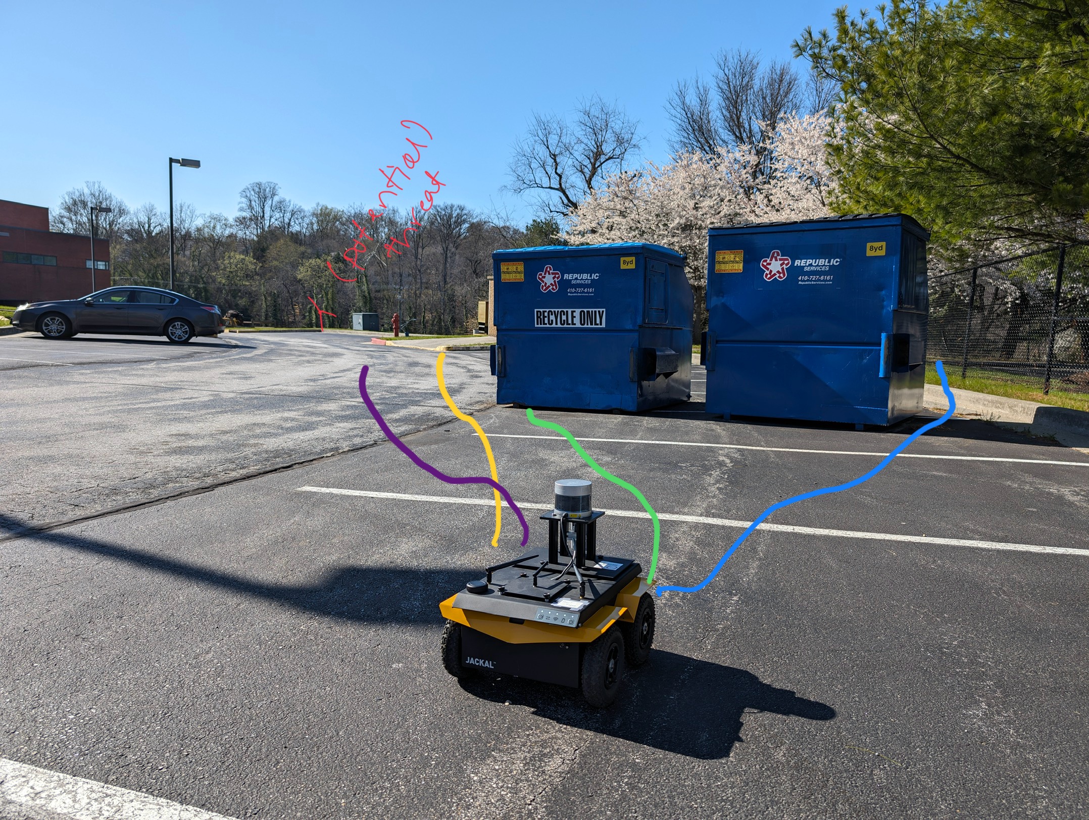
(a)

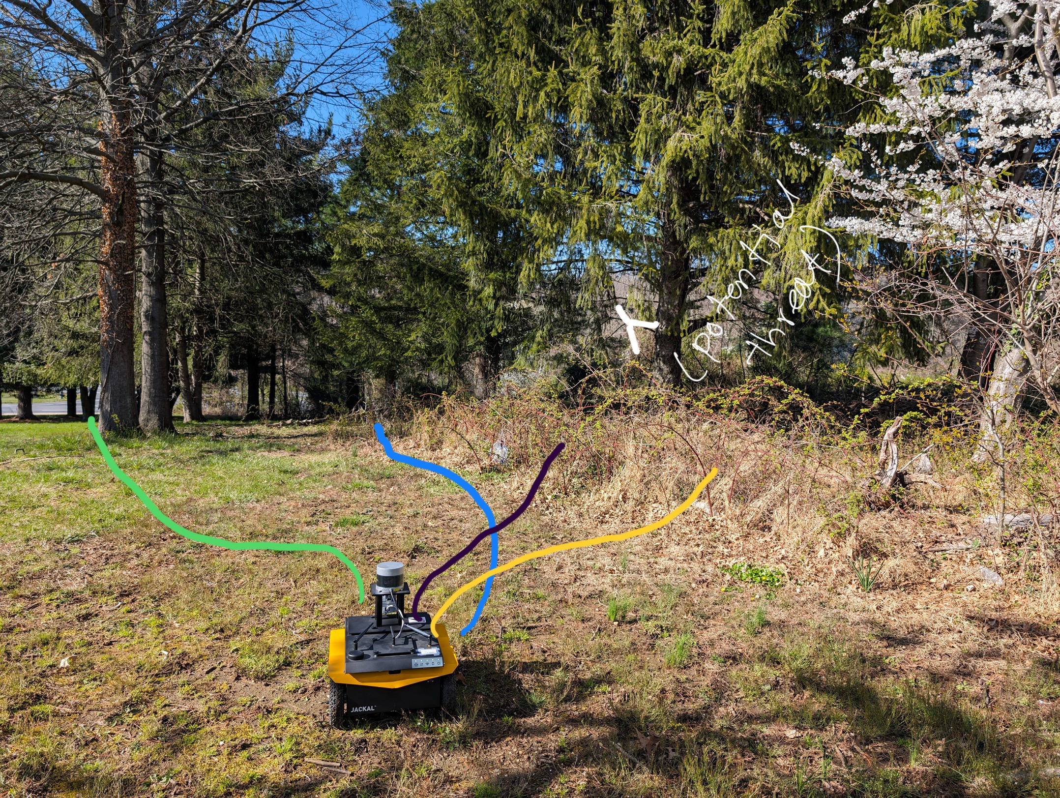
(b)

(c)

Figure 3: Comparison of navigation strategies in diverse outdoor settings (See 6.4). (a) Scenario 1, (b) Scenario 2, (c) Scenario 3. Paths indicate the trajectories taken by different systems, with EnCoMP (blue) demonstrating more optimized routes that effectively leverage cover while minimizing threat exposure, in contrast to CoverNav (green), VAPOR (purple), and VERN (yellow).

Metrics	Methods	Scen. 1	Scen. 2	Scen. 3
Success	CoverNav	85	83	81
Rate (%)	VAPOR	87	85	84
	VERN	88	86	85
	EnCoMP(Ours)	95	93	91
Navigation	CoverNav	40.0	42.5	45.0
Time (s)	VAPOR	38.5	40.0	42.0
	VERN	39.0	41.0	43.5
	EnCoMP(Ours)	32.0	34.5	36.0
Trajectory	CoverNav	14.0	14.5	15.0
Length (m)	VAPOR	13.5	14.0	14.5
	VERN	13.8	14.3	14.8
	EnCoMP(Ours)	11.0	12.0	12.5
Threat	CoverNav	22.5	25.0	27.5
Exposure (%)	VAPOR	20.0	22.5	25.0
	VERN	18.5	21.0	23.5
	EnCoMP(Ours)	10.5	12.0	14.5
Cover	CoverNav	65.0	62.5	60.0
Utilization (%)	VAPOR	67.5	65.0	62.5
	VERN	70.0	67.5	65.0
	EnCoMP(Ours)	85.0	82.5	80.0

Table 1: Comparative Analysis: EnCoMP vs. SOTA methods across three scenarios, highlighting superior performance in metrics such as success rate, navigation time, threat exposure, and cover utilization.

7 Conclusion, Limitations, and Future Directions

In this work, we presented EnCoMP, an enhanced covert maneuver planning framework that combines multi-modal perception and offline reinforcement learning to enable autonomous robots to navigate safely and efficiently in complex environments. Our approach introduces several key contributions, including a multi-modal perception pipeline that generates high-fidelity cover, threat, and height maps, an offline reinforcement learning algorithm that learns robust navigation policies from real-world datasets, and an effective integration of perception and learning components for informed decision-making. However, there are a few limitations to our current approach. First, the performance of EnCoMP relies on the quality and diversity of the real-world dataset used for training. While we have collected a substantial amount of data, there may still be scenarios or environments that are not well-represented in the dataset. Second, our approach assumes that the environment is static during navigation, which may not always hold in real-world scenarios. Dynamic obstacles or changing terrain conditions could impact the effectiveness of the learned policy.

Future research directions include extending EnCoMP to handle dynamic environments by incorporating online adaptation mechanisms into the reinforcement learning framework. Additionally, we plan to investigate the integration of active perception techniques, such as active mapping or exploration, to allow the robot to actively gather information about the environment during navigation. Another opportunity for future work is to explore the use of meta-learning approaches to enable the rapid adaptation of the learned policy to new environments or mission requirements. Furthermore, we plan to validate the performance of EnCoMP on a wider range of real-world terrains and scenarios, including more diverse vegetation types, weather conditions, and mission objectives.

References

- Ajai et al. [2019] S. Ajai, J. Ajith, S. Arjun, and S. Sebastian. An extensive survey on potential field based path planning for autonomous mobile robot. In International Conference on Intelligent Computing, Instrumentation and Control Technologies (ICICICT), pages 1004–1009, 2019.
- Brown and Davis [2019] A. Brown and E. Davis. Autonomous robots for search and rescue missions. In IEEE International Conference on Robotics and Automation (ICRA), 2019.
- Chebotar et al. [2019] Y. Chebotar, A. Handa, V. Makoviychuk, M. Macklin, J. Issac, N. Ratliff, and D. Fox. Closing the sim-to-real loop: Adapting simulation randomization with real world experience. In IEEE International Conference on Robotics and Automation (ICRA), 2019.
- Chen and Wang [2018] X. Chen and L. Wang. Supervised learning for traversable terrain classification. IEEE Transactions on Robotics, 2018.
- contributors [2024] Wikipedia contributors. Bresenham’s line algorithm — Wikipedia, the free encyclopedia, 2024. [Online; accessed 24-March-2024].
- Fan et al. [2020] Xinyi Fan, Zezhou Wang, Yuhang Zhang, Jiahao Liang, Wei Zhang, and Siwei Lyu. Learning stealth behaviors with multi-objective deep reinforcement learning. arXiv preprint arXiv:2006.10593, 2020.
- Fujimoto et al. [2019] S. Fujimoto, D. Meger, and D. Precup. Off-policy deep reinforcement learning without exploration. In International Conference on Machine Learning, pages 2052–2062, 2019.
- Garcia and Perez [2017] M. Garcia and L. Perez. Conservative navigation strategies for autonomous robots. Robotics and Autonomous Systems, 2017.
- Gupta and Sharma [2018] R. Gupta and S. Sharma. Efficient navigation in cluttered environments. In IEEE/RSJ International Conference on Intelligent Robots and Systems (IROS), 2018.
- Hansen et al. [2021] N. Hansen, Y. Sun, P. Abbeel, A.A. Efros, L. Pinto, and X. Wang. Self-supervised policy adaptation during deployment. In International Conference on Learning Representations (ICLR), 2021.
- Hossain et al. [2023] Jumman Hossain, Abu-Zaher Faridee, Nirmalya Roy, Anjan Basak, and Derrik E Asher. Covernav: Cover following navigation planning in unstructured outdoor environment with deep reinforcement learning. In 2023 IEEE International Conference on Autonomic Computing and Self-Organizing Systems (ACSOS), pages 127–132. IEEE, 2023.
- Kalashnikov et al. [2021] D. Kalashnikov, A. Irpan, P. Pastor, J. Ibarz, A. Herzog, E. Jang, D. Quillen, E. Holly, M. Kalakrishnan, V. Vanhoucke, and S. Levine. Offline reinforcement learning for efficient and robust robot manipulation. In IEEE International Conference on Robotics and Automation (ICRA), 2021.
- Kim and Park [2018] T. Kim and J. Park. Online reinforcement learning for outdoor navigation. Journal of Field Robotics, 2018.
- Kumar et al. [2020] Aviral Kumar, Aurick Zhou, George Tucker, and Sergey Levine. Conservative q-learning for offline reinforcement learning. Advances in Neural Information Processing Systems, 33:1179–1191, 2020.
- Lee and Kim [2017] J. Lee and S. Kim. Stealth navigation using pre-defined environmental models. In IEEE/RSJ International Conference on Intelligent Robots and Systems (IROS), 2017.
- Levine et al. [2020a] Sergey Levine, Aviral Kumar, George Tucker, and Justin Fu. Offline reinforcement learning: Tutorial, review, and perspectives on open problems. arXiv preprint arXiv:2005.01643, 2020a.
- Levine et al. [2020b] S. Levine, A. Kumar, G. Tucker, and J. Fu. Offline reinforcement learning: Tutorial, review, and perspectives on open problems. arXiv preprint arXiv:2005.01643, 2020b.
- Li et al. [2016] B. Li, T. Zhang, and T. Xia. Lidar-based 3d object detection for autonomous vehicles. In IEEE Intelligent Vehicles Symposium (IV), 2016.
- Liu and Chen [2020] J. Liu and Y. Chen. Reinforcement learning for autonomous navigation: A survey. IEEE Transactions on Intelligent Transportation Systems, 2020.
- Mandlekar et al. [2020] A. Mandlekar, F. Ramos, B. Boots, L. Fei-Fei, A. Garg, and D. Fox. Iris: Implicit reinforcement without interaction at scale for learning control from offline robot manipulation data. In IEEE International Conference on Robotics and Automation (ICRA), pages 4414–4420, 2020.
- Marzouqi and Jarvis [2006] M.A. Marzouqi and R.A. Jarvis. Covert robotics: Covert path planning in unknown environments. In Australasian Conference on Robotics and Automation (ACRA), 2006.
- Mendonça et al. [2018] Matheus RF Mendonça, Heder S Bernardino, and Raul Fonseca Neto. Reinforcement learning with optimized reward function for stealth applications. Entertainment Computing, 25:37–47, 2018.
- Nguyen and Tran [2019] A. Nguyen and H. Tran. Terrain traversability analysis using supervised learning. In IEEE International Conference on Robotics and Automation (ICRA), 2019.
- Niroui et al. [2019] Fatemeh Niroui, Kaiyu Zhang, Zoe Kashino, and Goldie Nejat. Deep reinforcement learning robot for search and rescue applications: Exploration in unknown cluttered environments. IEEE Robotics and Automation Letters, 4(2):610–617, 2019.
- Papadakis [2013] Pangiotis Papadakis. Terrain traversability analysis methods for unmanned ground vehicles: A survey. Engineering Applications of Artificial Intelligence, 26(4):1373–1385, 2013.
- Patel and Shah [2019] K. Patel and D. Shah. Deep reinforcement learning for robot navigation. In IEEE International Conference on Robotics and Automation (ICRA), 2019.
- Patel and Singh [2016] R. Patel and T. Singh. Stealth navigation in known environments. Journal of Field Robotics, 2016.
- Prudencio et al. [2023] Rafael Figueiredo Prudencio, Marcos ROA Maximo, and Esther Luna Colombini. A survey on offline reinforcement learning: Taxonomy, review, and open problems. IEEE Transactions on Neural Networks and Learning Systems, 2023.
- Sathyamoorthy et al. [2020] A.J. Sathyamoorthy, U. Patel, T. Guan, and D. Manocha. Frozone: Freezing-free, pedestrian-friendly navigation in human crowds. IEEE Robotics and Automation Letters, 5(3):4352–4359, 2020.
- Sathyamoorthy et al. [2022] A.J. Sathyamoorthy, K. Weerakoon, T. Guan, J. Liang, and D. Manocha. Terrapn: Unstructured terrain navigation using online self-supervised learning. In IEEE/RSJ International Conference on Intelligent Robots and Systems (IROS), pages 7197–7204, 2022.
- Sathyamoorthy et al. [2023] Adarsh Jagan Sathyamoorthy, Kasun Weerakoon, Tianrui Guan, Mason Russell, Damon Conover, Jason Pusey, and Dinesh Manocha. Vern: Vegetation-aware robot navigation in dense unstructured outdoor environments. In 2023 IEEE/RSJ International Conference on Intelligent Robots and Systems (IROS), pages 11233–11240. IEEE, 2023.
- Singh and Gupta [2019] V. Singh and A. Gupta. Outdoor navigation using online reinforcement learning. In IEEE/RSJ International Conference on Intelligent Robots and Systems (IROS), 2019.
- Smith and Johnson [2018] J. Smith and M. Johnson. Reconnaissance robots for military applications. Journal of Military Robotics, 2018.
- Tews and Sukhatme [2004] Ashley Tews and Gaurav S Sukhatme. Avoiding detection by abandoning perfect concealment. In IEEE/RSJ International Conference on Intelligent Robots and Systems (IROS), pages 1268–1273. IEEE, 2004.
- Tobin et al. [2017] J. Tobin, R. Fong, A. Ray, J. Schneider, W. Zaremba, and P. Abbeel. Sim-to-real transfer in reinforcement learning for robotics. IEEE Robotics and Automation Letters, 2017.
- Weerakoon et al. [2022] K. Weerakoon, A.J. Sathyamoorthy, U. Patel, and D. Manocha. Terp: Reliable planning in uneven outdoor environments using deep reinforcement learning. In IEEE International Conference on Robotics and Automation (ICRA), pages 9447–9453, 2022.
- Weerakoon et al. [2023] Kasun Weerakoon, Adarsh Jagan Sathyamoorthy, Mohamed Elnoor, and Dinesh Manocha. Vapor: Holonomic legged robot navigation in outdoor vegetation using offline reinforcement learning. arXiv preprint arXiv:2309.07832, 2023.
- Wilson and Taylor [2020] G. Wilson and H. Taylor. Surveillance robots: A survey. Robotics and Autonomous Systems, 2020.
- Zhang and Singh [2017] J. Zhang and S. Singh. Lidar-based terrain classification for autonomous driving. Journal of Field Robotics, 2017.