Influence of pressure anisotropy and non-metricity parameter on mass-radius relation and stability of millisecond pulsar in gravity
Abstract
In this study we explore the astrophysical implications of pressure anisotropy on the physical characteristics of millisecond pulsars within the framework of gravity. Starting off with the field equations for anisotropic matter distributions, we adopt the physically salient Durgapal-Fuloria ansatz together with a well-motivated anisotropic factor for the interior matter distribution. This leads to a nonlinear second order differential equation which is integrated to give the complete gravitational and thermodynamical properties of the stellar object. The resulting model is subjected to rigorous tests to ensure that it qualifies as a physically viable compact object within the -gravity framework. We study in detail two factors, one being non-metricity (gravitational interaction) and the other the pressure anisotropy (matter variation) and their contributions to the mass, radius and stability of the star. Our analyses indicate that our models are well-behaved, singularity-free and can account for the existence of a wide range of observed pulsars with masses ranging from 2.08 to 2.67 , with the upper value being in the so-called mass gap regime observed in gravitational events such as GW190814. A novel finding of this work is two-fold: an increase in the non-metricity factor (fixed anisotropy) leads to a spectrum of pulsars with radii ranging from a minimum of 10 km whereas a variation in anisotropy (fixed non-metricity) restricts the radii to a narrow window between () km for a 450 Hz pulsar. In addition, contributions from anisotropy outweigh the impact of nonmetricity in predicting the masses of pulsars with the ratio, for low mass pulsars.
1 Introduction
The first detection of a pulsar, aptly named LGM-1, by Jocelyn Bell in 1967 created quite a stir amongst her collaborators [1]. The regularity of the signals emanating from the source led them to believe that it could be artificially generated, hence the reference to Little Green Men 1 or LGM-1. Today we know that Bell had discovered a pulsar which is a rapidly rotating neutron star with a period of 1.3373 seconds. The neutron star itself is born out of a cataclysmic supernova explosion. Pulsars occupy an important place in observational astrophysics as they serve as natural laboratories for probing the nature of superdense matter, gravitational waves [2, 3, 4] and the end-states of gravitational collapse. Pulsars such as Cen X-, SAX J, Vela X- and PSR J have been extensively studied in the literature. Cen-X- was serendipituously discovered when rocket-borne detectors were trained upon X-ray sources Sco XR- and Tau XR-. X-rays were detected from the direction of the constellations Vela and Lupus in which the sources Vel XR- and Lup XR- were respectively located with the new source Cen-X- inhabiting the constellation Centaurus [5].
The pioneering work of Bowers & Liang [6] cast light on the impact of anisotropic stresses in relativistic compact objects. This seminal paper extended Bondi’s earlier work on isotropic configurations to include pressure anisotropy without the imposition of an equation of state (EOS). The key findings of their investigation were the prediction of higher surface redshifts and the maximum allowable mass of gravitating bodies in the presence of unequal radial and transverse stresses. It was well-known that physical processes such as pion condensation [7, 8], neutrino transport [9], superconducting states, amongst others, give rise to anisotropy within the stellar core. These processes play a significant role at ultra-high densities, especially during the last stages of gravitational collapse. In their review article, Herrera and Santos highlighted the impact of anisotropy in radiating stars [10]. The highlight of their work signified the modification of the adiabatic index in both the Newtonian and post-Newtonian approximations which generalises the classic stability result obtained by Chandrasekhar for isotropic matter distributions [11]. The dynamical (in)stability of the collapsing body is affected by the sign of the anisotropic factor as well as the gradient of the radial pressure. In a more recent study, Herrera demonstrated the instability of the pressure isotropy condition in fluids losing hydrostatic equilibrium [12]. It was shown that an initial isotropic matter distribution, upon leaving hydrostatic equilibrium, will evolve into an anisotropic regime. In particular, the appearance of the radial pressure term in the TOV equation (which is absent in the Newtonian analogue) plays a crucial role in the anisotropisation of the collapsing fluid.
Recently, there has been an exponential growth of exact solutions of the Einstein field equations describing anisotropic compact objects. A popular approach to close the system of coupled equations is to employ a metric ansatz for one of the gravitational potentials and impose a governing equation that dictates the symmetry and/or nature of the spacetime (for example, the Karmarkar condition for embedding class I spacetimes [14, 16, 13, 15]), an EOS (which relates the radial pressure and energy density), complexity-free condition, amongst others. Various EOS’s ranging from the simple linear EOS (), through to the MIT bag model, the polytropic EOS and the CFL EOS have been employed to complete the gravitational and thermodynamical behaviour of the models. The sophistication of the plethora of EOS’s has grown with experimental results from particle physics. Numerous stellar models arising from the imposition of an EOS have revealed the impact of the bag constant, quark interactions and quark energies. In a recent article, the authors considered quarks to form Cooper pairs which obeyed a color–flavor-locked (CFL) EOS which formed the stellar fluid of strange stars admitting masses in the vicinity of 3.61 [17]. They further provided evidence that the 3-flavor strange quark matter (SQM) in the CFL phase exhibits complete stability in comparison to for strange quark masses, . In addition, the stability of SQM increases with a decrease in . Their study of observed compact objects showed that PSR J1614-2230 and PSR J0740+6620 are found to be anisotropic in nature. In a more recent study, Mohanty et al. employed a total of 60 EOS’s to investigate the impact of anisotropy in neutron stars [18]. By using a numerical methodology, the researchers demonstrated the feasibility of producing neutron star masses above 2.0 within the framework of general relativity (GR) by influencing the magnitude of anisotropy present in the stellar core.
The inclusion of pressure anisotropy via gravitational decoupling (GD) has been successfully implemented to produce a wide spectrum of compact stellar objects. The basis of the GD framework is to introduce an additional source via the energy-momentum tensor of the standard Einstein field equations. The additional source term mimics anisotropy within the stellar configuration. The so-called minimal geometric deformation (MGD) technique [19] and its generalisation, referred to as complete geometric deformation (CGD) [20] have led to anisotropic analogues of well-known isotropic solutions of the Einstein field equations. It must be pointed that while the isotropic seed solution may suffer various pathologies, their anisotropic counterparts obtained via MGD or CGD may represent realistic compact stellar objects. It has been shown that the decoupling constant influences stellar characteristics such as mass-radius relations, stability and the upper mass limit of compact objects [21, 23, 22].
Inspired by the observations of the LIGO-VIRGO collaboration of events such as GW170817 and GW190814, researchers have renewed their efforts in modeling the compact objects involved in binary mergers which are sources for gravitational waves. In particular, the gravitational wave event GW190814 indicates that the signals were generated by a fusion of a black hole with a mass ranging from 22.2 to 24.3 and a compact object with a mass ranging from 2.50 to 2.67. On the other hand, the GW170817 event is ascribed to the merger of two neutron stars with masses in the range 0.86 - 2.26 . In order to achieve stellar masses greater than 2 in standard GR without invoking exotic matter distributions or rotation, theorists have ventured into modified gravity theories. One such popular theory is the -gravity which has proved to be quite diverse in its predictive power, both in the astrophysical and cosmological frontiers. A power-law form for the metricity factor which takes the form was first proposed by Capozziello and D’Agostino [24]. A special case of the Capozziello and D’Agostino ansatz, i.e., a linear form of metricity scalar (taking ) was employed by Maurya et al. [mauryajcap] to study compact objects with anisotropic pressure by the anisotropisation of the Tolman IV solution via gravitational decoupling. The ensuing models described physically viable stellar structures including a range of stars endowed with masses of the order of 1.2 - 2.26 . In particular, this work demonstrated that contributions from the metricity factor, predict larger stars. By adopting a singularity-free form for the gravitational potentials described by the Tolman-Kuchowicz ansatz, Bhar et al. modeled anisotropic hybrid stars in which the stellar fluid comprised of a superposition of strange quark matter (SQM) and ordinary baryonic matter (OBM) distributions within the gravity framework [25]. In addition, they adopted the MIT bag model EOS to complete the gravitational behaviour of the model. Their models were singularity-free and covered a range of stellar masses including compact objects in the range required by the secondary component of the GW 190814 event [26]. The mass-gap conundrum arising in gravitational events has presented researchers with various challenges over the recent years. The latest candidate is a pulsar of mass 2.09 to 2.71 which forms one component of a binary system observed by the MeerKat survey [27].
In a recent paper, Maurya et al. [28] employed a quadratic EOS together with a linear form for to study compact objects within the MGD framework. They showed that the most robust model which accounts for a wide spectrum of stars, especially compact objects with masses in the regime predicted by GW190814 is the one incorporating a superposition of linear and quadratic contributions from the stellar density. In order to study the influence of the quadratic term arising in , where in the limiting case of , we regain classical GR, Bhar et al. modeled charged compact objects with anisotropic stresses in the interior [29]. They demonstrated that their models were sensitive to the EOS parameter, metricity, charge, and the bag constant. In addition, they noted that the quadratic contribution from results in the lowering of the density, radial pressure, electric field, and sound speeds. The novelty of their work lies in the ability of increasing the magnitude of the anisotropy via the quadratic presence in without invoking gravitational decoupling or any exotic scalar field or matter distributions, including dark energy. For a recent review on gravity, we refer the reader to [30] for more details. In their recent work, Capozziello et al. [31] have demonstrated that gravitational waves generated in non-metricity-based gravity exhibit similar characteristics to those in torsion-based gravity [32, 33, 34, 35, 36]. Consequently, distinguishing between these gravitational waves and those predicted by General Relativity based solely on wave polarization measurements becomes challenging. This distinction contrasts with the behavior observed in curvature-based gravity [37, 38, 39, 40, 41, 42, 43, 44], where an additional scalar mode is always present when .
The paper is organized as follows: Sec. 2 presents a concise overview of the underlying principles of modified -gravity theory. Moving on to Sec. 3, an exact anisotropic solution in -gravity is derived. The determination of boundary conditions is addressed in Sec. 4, where the interior spacetime is matched with the exterior spacetime, specifically the Schwarzschild (Anti-) de Sitter spacetime, at the pressure-free boundary. Sec. 5 delves into the investigation of the physical viability of the stellar model, focusing on the behavior of various thermodynamic variables such as energy density, radial and tangential stresses, and the anisotropic parameter. In Secs. 6 and 7, the maximum mass and radii predictions for different neutron stars are discussed, along with stability analysis using the adiabatic index and Harrison-Zel’dovich-Novikov criteria, respectively. Finally, Sec. 8 provides concluding remarks on our findings.
2 Modified -gravity theory
The processes for the modified gravity technique are as follows [46, 45]: the action for -gravity with matter sources is given by
| (2.1) |
where the symbol denotes the Lagrangian density for matter distribution while represents a nonmetricity scalar. The energy-momentum tensor connected to Lagrangian is expressed as
| (2.2) |
The tensor for nonmetricity term is calculated as
| (2.3) |
where, defines the affine connection, further it is defined as
| (2.4) |
with
| (2.5) |
where , , , and are known as the disformation, Levi-Civita connection, torsion tensor and the contortion tensors respectively. Further, the anti-symmetric part of the affine connection can be defined as . This last expression also described by the torsion tensor .
Finally, the non-metricity scalar expression can be cast as
| (2.6) |
The above equation provides a non-metricity conjugate. The corresponding tensor is defined as
| (2.7) |
Here, and are the two independent traces. Both the traces can be defined by the following relation
| (2.8) |
To get the appropriate field equations for -gravity, it is required to vary the action (2.1) with respect to the metric tensor . Thus, one can obtain the gravity field equations as follows:
| (2.9) |
where . In addition, Eq. (2.1) can be used to construct an extra connection constraint. Consequently, It is defined as
| (2.10) |
Other restrictions, particularly torsion-free and curvature-free, permits us to represent the affine connection as
| (2.11) |
where, can be obtained for coincident gauge. As a result, from Eq. (2.3), we have the following expression
| (2.12) |
On the other hand, we consider the spherically symmetric metric of the form,
| (2.13) |
where and are functions of only.
The non-metricity scalar for the spacetime (2.13) is given by,
| (2.14) |
Furthermore, we consider the matter distribution to be anisotropic. In this case, the source is given as,
| (2.15) |
Then the non-zero components of the energy-momentum tensor are
| (2.16) |
For the spherically symmetric metric (3), the final form of the field equations (assuming that the affine connection is zero) can be written as,
| (2.17) | |||
| (2.18) | |||
| (2.19) | |||
| (2.20) |
In order to proceed with obtaining models of compact stellar objects, we assume that the interior matter distribution, under the influence of gravity, is endowed with anisotropic pressure. The results obtained by Zhao [46] on the compatibility of static SS spacetimes with the coincident gauge are very significant. In light of Zhao’s findings, with the affine connection being zero in the specified coordinate framework, and further enforcing the requirement that the -gravity theory yields vacuum solutions, particular , it is possible to deduce that the off-diagonal component as given by Eq. (2.20),
| (2.21) |
where, is given by Eq. (2.14).
Furthermore, the equations of motion, when combined with the diagonal components (2.21), lead to being zero. This finding suggests that choosing initially will lead to an inconsistent system of equations of motion. If the function is not linear with respect to , then the metric equation (2.13) combined with an affine connection does not provide an acceptable solution for the equations of motion. The nonexistence of static SS vacuum solutions in theory does not always indicate the absence of such solutions. Instead, it implies that the SS coordinate system does not align with the coincident gauge. To get SS solutions, one needs to think about a more extensive definition of the static SS metric. For a comprehensive understanding of this aspect and to get a detailed explanation, please refer to Ref. [46].
Furthermore, the research carried out by Avik & Loo [47] indicates that the presence of classical events cannot be guaranteed within the framework of the symmetric teleparallel theory. However, it relies on the distinct attributes of the model. The authors give further evidence that supports the correspondence between the energy conservation criteria and the field equation of the affine connection within the framework of theory. It is crucial to note that, except the linear form of , the non-linear models fail to satisfy the energy conservation criterion or, equivalently, the ensuing field equation for all spacetime geometries, as long as the variable stays constant. In this regard, Wang et al. [48] also proved that the exact Schwarzschild solution is only valid when the functional form of is linear, and they have imposed constraints on its derivation and limitation. Together with a deep-dive into related work in the existing literature and the compatibility of the proposed solution, we have assumed
| (2.22) |
where and are constants.
The set of equations for motion that results when Eqs. (2.13) and (2.22) are replaced into Eqs. (2.17) - (2.19) are as follows:
| (2.23) | |||
| (2.24) | |||
| (2.25) |
The mass function under -gravity regime can be calculated with the aid of the formula,
| (2.26) |
The linear combination of (2.23)-(2.25) yields,
| (2.27) |
Surprisingly the equation (2.27) corresponds to the conservation formula in General Relativity (GR) and is often referred to as the TOV equation in the -gravity theory [50, 49, 48]. Our objective is to find an exact solution to the -gravity field equations (2.23)-(2.25) by considering an anisotropic distribution of matter which we provide in the next section.
3 Exact anisotropic solution in -gravity
As we can see that we have five unknowns: , , , , and and three independent equations. It is very important to mention that various techniques, including the MIT bag model or polytropic EOS, Karmarkar conditions, and complexity factor conditions, have been used to solve the system of equations in -gravity along with various modified gravity theories. On the other hand, Harko and his collaborators [51, 52, 53] investigated the most general solution of Einstein’s gravitational field equations describing spherically symmetric and static anisotropic stellar type configurations using particular form of anisotropy and density profile. Therefore, we use the same methodology to solve the -gravity system to determine the most general exact solution for an anisotropic distribution of matter. To achieve this objective, we use the anisotropic condition in equations (2.24) and (2.25), which is derived by subtracting equation (2.18) from equation (2.19). The pressure anisotropy condition in -gravity is obtained in the following manner:
| (3.1) |
The above equation contains three unknowns namely , , and .
To solve the master equation (3.1), we shall consider the following physically valid expression for variable given by the Durgapal-Fuloria ansatz [54]:
| (3.2) |
where is a constant. The Durgapal-Fuloria ansatz has been widely used to model superdense stars in classical general relativity as the resulting stellar models display various salient features with regards to regularity, stability and causality. It was shown that the ensuing models could have masses which makes it suitable to model the secondary component of gravitational events such as GW190814. Using Eq. (3.2), the anisotropy condition (15) along with transformation reduce to
| (3.3) |
Since the above equation involves two undetermined unknowns and , we have to specify a viable expression for which yields the closed-form solution which we seek. Employing physical considerations based on regularity together with some mathematical manipulation, we conceive the following expression for ,
| (3.4) |
Here is a positive constant. To ensure positive anisotropy throughout the model, the factor:
, must be positive. This condition gives the constraint as:
| (3.5) |
By plugging the expression of in Eq.(3.3), we get a general second order ODE in ,
| (3.6) |
where, . If we look closely at Eq.(3.6), we note that setting:
satisfies the above equation.
Then the most general solution can be found by assuming: as a particular solution of Eq.(3.6). Let us assume, is a general solution of Eq.(3.6). We then obtain
| (3.7) |
where, and are arbitrary constants of integration. After integration of the above equation, we get
| (3.8) |
where, new arbitrary constants and have been introduced while
The expressions for energy density and pressures may be derived using equations (2.23)-(2.25) along with Eqs. (3.2) and (3.8) as,
| (3.9) | |||
| (3.10) | |||
| (3.11) |
where, , .
4 Boundary Condition
The junction conditions are an essential part of bounded astrophysical stellar systems, which could be determined by matching the interior spacetime with the exterior spacetime at the pressure-free boundary. In the linear -gravity, the Schwarzschild (Anti-) de Sitter spacetime is a suitable exterior spacetime, which can be given as
| (4.1) |
where indicates a cosmological constant () while is the total mass of object with and . For smooth matching, we use the Israel-Darmois junction conditions, which are mainly: (i) Smooth matching of metric functions at the boundary ), (ii) vanishing of radial pressure at the stellar boundary . Mathematically, we can express theses as:
| (4.2) | |||||
| (4.3) | |||||
| (4.4) |
The constants and will be obtained via the above-mentioned matching conditions.
5 Physical Analysis
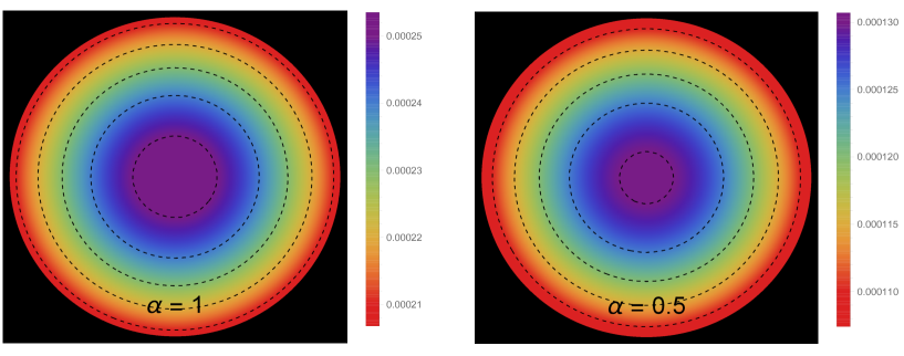
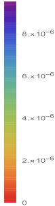
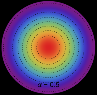
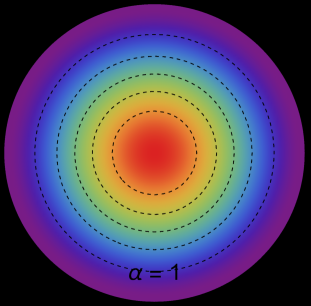
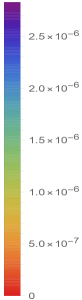
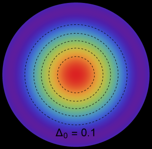
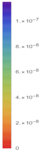
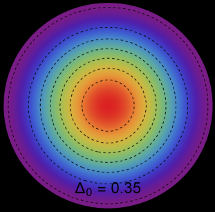
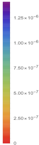
In this section, we investigate the physical viability of our stellar model in terms of the behaviours of the thermodynamical variables, viz., energy density, radial and tangential stresses and the anisotropic parameter. An inspection of Figure 1, reveals that the energy density is regular at each interior point of the configuration. The energy density is a monotonically decreasing function of the radial coordinate, attaining a maximum value at the centre of the self-gravitating object. The key difference in the left and right panels of Figure 1 is the change in magnitude of the parameter, while the anisotropy factor, is fixed. We observe that an increase in the magnitude of leads to a higher core density. The effect of the parameter is to accentuate the density in the central regions of the star, ie., there is a ’squeezing’ of more matter in central, concentric shells. As one moves away from the centre, towards the surface layers of the star, a change in has no perceptible effect on the stellar density.
We now turn our attention to Figure 2 in which we have plotted the radial pressure as a function of the radial coordinate. The left two panels display the variation of the radial pressure for and respectively with the anisotropy parameter, held constant. As with the trend in the density, we note that the radial pressure is continuous everywhere inside the star and decreases monotonically with increasing radial coordinate. In the right two panels, we have varied the anisotropy parameter (left image we set and on the extreme right ) while the parameter is fixed. For we observe that the radial pressure in the central region is higher than in the case of by an order of . An increase in the anisotropic factor seems to relax the fluid particles with this property being more pronounced in the central regions of the star.
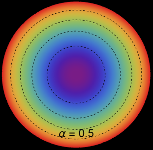
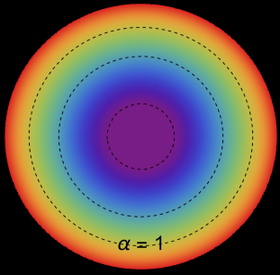
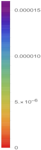
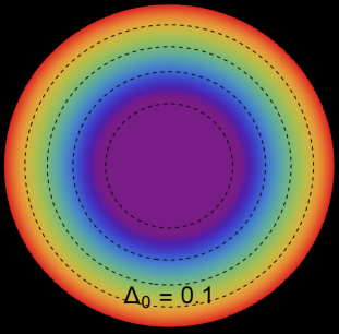
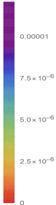
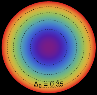
The trend in the anisotropy parameter, is portrayed in Figure 3. We recall that , with signifying a repulsive force due to radial stresses dominating the transverse stresses within the stellar configuration. This repulsive force helps stabilise the compact object against the inwardly directed gravitational force. In the left two panels of Figure 3, we have varied while holding constant. The anisotropy is well-behaved and vanishes at the centre of the configuration. Anisotropy grows in magnitude as one moves outwards towards the boundary which culminates in greater stability of the surface layers of the star. We note that an increase of from to , results in the doubling of the anisotropy within the stellar body. The two right figures in Figure 3 show the variation of with a variation in while is fixed. As increases, we observe a factor of increase in anisotropy at each interior point of the gravitating body. The role of is to render the stellar fluid more anisotropic, ie. there is a larger deviation between the radial and tangential stresses which helps stabilise the star. Effectively, can be a measure of physical processes such as phase transitions, neutrino and electron transport within the stellar interior as well as dissipation.

6 Prediction of maximum mass and radii for different Neutron stars
Pulsars are neutron stars that can emit periodic and strong electromagnetic signals as pulses arising from their high magnetic fields and rotational property. Large rotational frequencies of such pulsars indicate that they should be highly compact. In general, pulsars can be found in binary systems where the massive neutron star can have one companion star. These binary systems subject to Kepler’s third law can provide measurements of mass [55, 56] utilizing time delay analysis of pulses. To study the effect of anisotropy in Durgapal-Fuloria model under gravity framework, we have chosen some pulsars which are PSR J074 + 6620 [57] with low mass star as companion, PSR J1810+1744 [58, 59] with very low mass star as companion, PSR J1959+2048 (the black widow) [60] with PSR J2215+5135 (the redback) [60] as companion and GW190814 [4] with a black hole as companion. This set of pulsars having masses greater than 2 are considered to be very massive. Inevitably the existence of such massive pulsars is supported by stiff EOS which allows comparatively larger values of pressure for different fixed values of energy density. In this scenario, the pressure dominates in the neutron star configuration and resists the gravitational collapse of the matter.
Measurements of radii of neutron stars seem more difficult and tricky [62, 61] with observational parameters as compared to the determination of their masses. Certainly, both the tidal deformability factor related to the detection of gravitational waves [63] and NICER measurements on hotspots [64, 65] of neutron surfaces have opened ways to determine radii of neutron stars. For instance, the radius of PSR J0740+6620 has been measured to be km [66] at 68% credibility from NICER and XMM-Newton observations of rotating patterns of hotspots. Another reliable way is to determine the radiation radius which is given by as a consequence of redshifted stars’ surface temperatures and luminosities occurring from the observed thermal emissions of neutron stars. For a physical star .
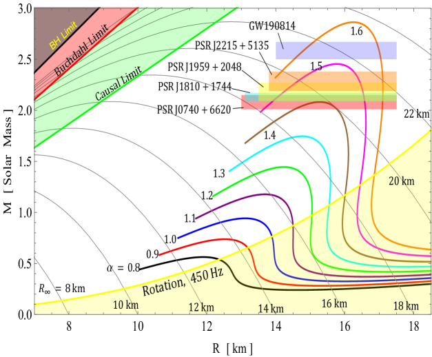
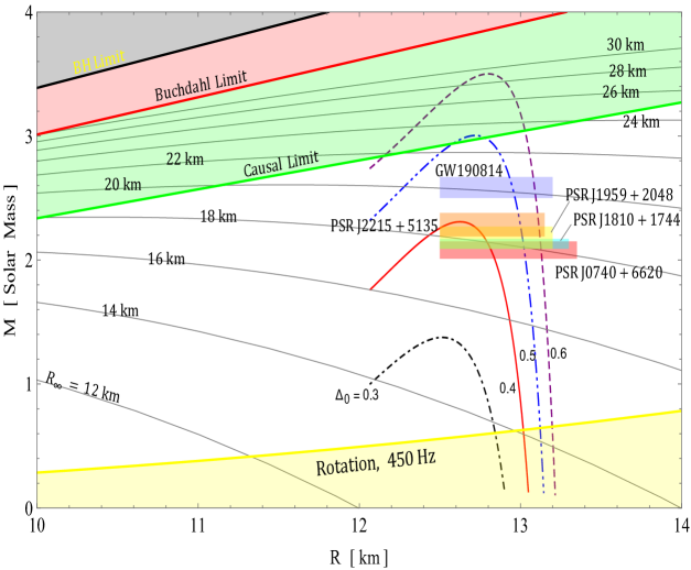
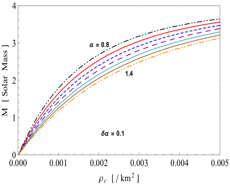
The determination of neutron star radii is a challenging task that can be eased by the progress in theoretical modeling. In this work we have developed a framework to construct models of pulsars based on the well-behaved Durgapal-Fuloria ansatz in gravity. Importantly, mass-radius curves are shown in Figure 4 for different values of for fixed anisotropy parameter (top panel) and for different values of anisotropy for fixed . It is to be noted that the curves correspond to the EOSs of matter via the TOV equation.
Contours of different fixed values of radiation radius are illustrated in Figure 4. The horizontal bands corresponding to the chosen pulsars have been shown in Fig 4. The curves which cross constraints like causality limit and Buchdahl limit and those do not intersect with the horizontal bands of pulsars can be excluded for radii measurements. This helps to predict the radii tabulated in Table 1.
In the top panel, the curves increase gradually towards a maximum peak and decrease sharply to a minimum thereafter remaining constant for increasing radii. This trend highlights the variation in radius for a range of different masses of neutron stars. We observe that neutron stars with a small mass () have larger radii for different values of . The intermediate part of curves shows the smaller change in the radii. As increases the peak of curves shifts upwards and horizontally towards the right. This means higher values lead to neutron stars with larger mass as well as larger radii. Evidently, curves with larger values of can be related to a stiffer EOS which supports the existence of massive neutron stars. The maximum masses and the corresponding radii for different values of in Table 2.
| () | (km) | () | (km) | ||
|---|---|---|---|---|---|
| 0.8 | 0.565 | 12.10 | 0.3 | 1.372 | 12.53 |
| 0.9 | 0.736 | 12.72 | 0.4 | 2.303 | 12.64 |
| 1.0 | 0.939 | 13.22 | 0.5 | 3.001 | 12.73 |
| 1.1 | 1.174 | 13.80 | 0.6 | 3.505 | 12.80 |
| 1.2 | 1.442 | 14.31 | - | - | - |
| 1.3 | 1.742 | 14.83 | - | - | - |
| 1.4 | 2.083 | 15.30 | - | - | - |
| 1.5 | 2.456 | 15.84 | - | - | - |
| 1.6 | 2.862 | 16.30 | - | - | - |
Furthermore, the top panel suggests that prediction of the radii of millisecond pulsars with a mass greater than 2 for a fixed value of anisotropy constant () is possible for . However, the bottom panel of Figure 4, implies that radii of very massive pulsars can be predicted for lower values of if anisotropy is increased to a sufficient amount. So, in gravity framework, there is a driving competition between and anisotropy to establish an impact on the stiffness of the EOS of matter. Hence, anisotropy has a significant influence on curves in gravity.
The intermediate linear part of curves goes to a certain height and sees a quick bend to go down with smaller changes in radii. The physical indication of the maxima of this bend is that matter within the neutron star is squeezed to its maximum limit. So, this peak provides the information on the maximum mass of the neutron star for a fixed value of and anisotropy. The maximum masses and the corresponding radii for different values of are in Table 2.
As compared to curves in Figure 4, similar kinds of curves with a maximum mass of 2.2 can be observed in earlier research work [67] based on variational methods and EOSs for nucleonic matter. Astashenok and Odintsov [68] conducted an investigation where they anticipated supermassive compact stars with masses ranging from and radii of roughly within the context of axion gravity. The presence of an axion “galo” around the star leads to a slower decay of the scalar curvature compared to vacuum gravity. In the study conducted by Nashed et al. [69], the authors explore the application of higher-order curvature theory to spherically symmetric spacetime solutions for the interior of stellar compact objects. The model successfully satisfies the required constraints for anisotropic compact stars, with particular emphasis on the Her X-1 star. The proposed model exhibits enhanced stability compared to analogous models in GR. Interestingly, the inclusion of hyperons in the EOS reduces the maximum mass effectively to 1.6 . In other works [71, 70], different EOSs such as AP1-4 [72], MS1-3 [73], PAL1-6 [74], GM1-3 [75] are utilized to plot curves which have similar type of patterns to curves in Figure 4 produced in gravity. It is worth mentioning that the EOSs such as MS2, PAL1, and AP3, AP4 are stiffer as these represent comparatively high mass neutron stars in the plot.
7 stability Analysis
7.1 Stability analysis via adiabatic index
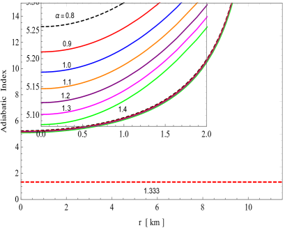
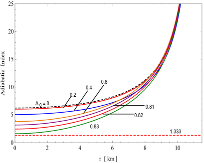
Now, we must assess the stability of the anisotropic stellar configuration. To do this, it is necessary to examine the adiabatic index () given by
| (7.1) |
The stability criterion for an isotropic fluid in the Newtonian limit is expressed as , as stated by Heintzmann and Bondi [77, 76] in their respective works on neutron stars and anisotropic fluids. The stability requirement for an anisotropic stellar model, deviates from the classic Chandrasekhar result for isotropic fluids [79, 78],
| (7.2) |
where primes are used to represent differentiation with respect to the radial coordinate, denoted as . The second component in Equation (7.2) accounts for the adjustments in the stability condition caused by the presence of anisotropy (), while the final term reflects relativistic adjustments.
From Figure (5), it is evident that the parameter and the anisotropy parameter significantly influence the limit for in the stability condition of an anisotropic star model. The left panel of Figure 5 illustrates that the value of increases as the value of decreases. This indicates that the parameter in the function determines the stability of the stellar structure. However, the value of cannot be arbitrarily high, despite other physical parameters such as pressure, density, casual limit and compactness exhibiting well-behaved characteristics within the model. In the given scenario, the left panel of Figure 5 demonstrates that the value of is more than 1.33 when is less than or equal to 13.8, which serves as the maximum limit for in order to obtain a stable model. In addition, the right panel of Figure 5 exhibits the same pattern as the left panel, indicating that an increase in corresponds to a decrease in the value of . This suggests that a model with significant anisotropy may result in an unstable model. In this scenario, it may be inferred that a stable star configuration cannot hold an arbitrarily high level of anisotropy. Observing the bottom panel of Figure 4, it is evident that the mass-radius relationship of our model fails to satisfy the casualty condition when . Based on the information shown in Figure 4 and 5, we can deduce that our model is stable when the value of is less than 0.5.
7.2 Stability analysis using the Harrison-Zel’dovich-Novikov criterion
In a previous study, Chandrasekhar [80] presented a way to determine the stability of a star system when subjected to radial perturbations. The perturbed physical parameters in this scenario, such as the metric functions, pressure, and density, are provided as follows:
| (7.3) | |||
| (7.4) |
The radial perturbations are modelled as exponential functions of the kind , where represents the characteristic frequency and the perturbations exhibit oscillatory behaviour. The oscillation’s stability is governed by the parameter . Therefore, we get from Eqs. (2.17) and (2.18),
| (7.5) |
The Lagrangian displacement, denoted by , is directly related to the radial velocity by the equation , where represents the world time.
Moreover, the fluctuation in energy density may be mathematically represented as
| (7.6) |
stating the conservation of the baryon number as
| (7.7) |
here, represents the radial adiabatic index.
By replacing equations (7.6) and (7.7) in equation (7.5), we find
| (7.8) |
which is reduced to a more basic or straightforward form
| (7.9) |
This has been referred to the pulsation equation in the literature.
Multiplying Eq. (7.9) by yields
| (7.10) |
as the “characteristic equation". This implies that the characteristic frequency is positive for a small radial oscillation that does not collapse. Moreover, Chandrasekhar’s computation is streamlined for the polytropic EOS, denoted as , as shown in references [81] and [82]. It is proven that for . Therefore, the mass may be expressed as a mathematical function of its central density, given by . Remarkably, we see that is a monotonically rising function of for , resulting in . The static stability criteria, also known as the Harrison-Zel’dovich-Novikov criterion, asserts that for an anisotropic stellar object to remain stable, the total mass () must increase as the centre density () increases.
In order to examine the condition for stability, we possess the following mathematical representations for the physical variables ,
| (7.11) | |||
| (7.12) | |||
| (7.13) |
From Figure 6, it is evident that mass is a monotonically increasing function of central density. Once again, Figure 6 demonstrates that the rate of change of mass in relation to the central density is positive and follows a linear pattern over the whole stellar area. Hence, the current model of anisotropic star satisfies the stability condition.
8 Concluding Remarks
In this paper, we have explored the impact of anisotropy on the mass, radius, and stability of pulsars within the framework of -gravity. By adopting the Durgapal-Fuloria ansatz described in (3.2), we derived a viable expression for the anisotropy function, denoted as . This expression allowed us to obtain a closed-form solution, as presented in (3.4). Our findings demonstrated that several compact objects, such as PSR J074+6620 [57], PSR J1810+1744 [58, 59], PSR J1959+2048 [60], PSR J2215+5135 [60], and GW190814 [4], are in good agreement with observational data. These pulsars serve as specific examples that highlight the significance of anisotropy in shaping their properties. Next, by utilizing the chosen metric functions, we proceeded to simplify the Einstein field equations and investigated the macroscopic characteristics of anisotropic pulsars within the framework of the theory under consideration. To account for the local anisotropy in pressure within the pulsars, we incorporated the Bower & Liang approach proposed in 1974 [6]. While there exists alternative formalisms such as the Horvat model [83] and the Cosenza model [84] that can also incorporate anisotropy within pulsars, the Bower-Liang model stands out for its simplicity. It assumes that the anisotropy is gravitationally induced and exhibits a nonlinear variation with radial pressure.
By considering the physical constraints, we have successfully aligned the interior solution with an exterior Schwarzschild (Anti-) de Sitter spacetime while fixing the constants and . Consequently, with the known values of these constant parameters, we further ascertained the masses and radii of pulsars. The models have been carefully analyzed to ensure they meet the necessary conditions for viability within the stellar fluid’s interior. Notably, the energy density within the configuration was regular at every point and decreases monotonically as the radial coordinate increases, reaching its maximum at the center of the self-gravitating object. Increasing the magnitude of the parameter led to a higher density in the core, effectively squeezing more matter into central, concentric shells. However, beyond the central region, changes in did not significantly affect the stellar density. The radial pressure as a function of the radial coordinate was examined in detail. We investigated two scenarios: one with and another with , while keeping the anisotropy parameter constant. Additionally, we explored the effects of varying the anisotropy parameter by considering and while keeping the parameter fixed. Similar to the density trend, we found that the radial pressure remains continuous throughout the star and decreased monotonically as the radial coordinate increased. Notably, when , the central region exhibited higher radial pressure compared to the case of by a factor of . Increasing the anisotropic factor appeared to result in a relaxation of the fluid particles, particularly in the central regions of the star. We delved into the characteristics of the anisotropy parameter, , where a positive indicates a repulsive force dominated by radial stresses that counteracts the inward gravitational force, thereby contributing to the stability of the compact object. By varying while keeping constant, we found that the anisotropy behaved smoothly, vanishing at the center of the configuration and increasing in magnitude towards the outer boundary, resulting in enhanced stability in the surface layers of the star. Moreover, doubling from to led to a doubling of anisotropy within the stellar body. When examining the variation of with changes in while remains fixed, we observed a tenfold increase in anisotropy at each interior point of the gravitating body as increases. The parameter plays a crucial role in rendering the stellar fluid more anisotropic, introducing a greater disparity between radial and tangential stresses, which ultimately aids in stabilizing the star.
Next, the Durgapal-Fuloria model in gravity had been developed to study the effect of anisotropy on pulsars. Specific pulsars, including PSR J074+6620, PSR J1810+1744, PSR J1959+2048, PSR J2215+5135, and GW190814, had been considered for their high masses. These massive pulsars are supported by EOSs that allow for larger pressure values at fixed energy density, preventing gravitational collapse. To analyze the mass-radius relationship, curves have been constructed for different values of (a parameter in the model) and anisotropy. The curves exhibited several notable features: the presence of contours representing fixed values of radiation radius, two bending parts at the top and bottom of the curves (with an almost linear part in the middle), and the dependence on both and anisotropy. The curves showed that neutron stars with smaller masses have larger radii, and increasing leads to neutron stars with larger masses and radii. The prediction of radii for pulsars with masses exceeding 2 is possible for certain values of and anisotropy. The maximum mass of a neutron star can also be inferred from the peak of the bending part in the curves. Comparisons with other studies using several methods and different EOSs have shown similar patterns in the curves. For instance, earlier research work by Togashi et al. [67], based on variational methods and EOSs for nucleonic matter, also exhibited curves with a maximum mass of 2.2 . In a study by Astashenok and Odintsov [68], supermassive compact stars with masses around and radii approximately were predicted within the framework of axion gravity. The presence of an axion “galo” around the star resulted in a slower decay of the scalar curvature compared to vacuum gravity. In contrast, Nashed et al. [69] conducted a study examining for sphercially symmetric anisotropic stellar models. within the framework of higher-order curvature theory, focusing specifically on the Her X-1 star. Their proposed model demonstrated enhanced stability compared to analogous models in GR. Interestingly, the inclusion of hyperons in the EOS effectively reduced the maximum mass to 1.6 . Other works, such as those by authors [71, 70, 72, 73, 74, 75], and the EOSs they utilized (e.g., AP1-4, MS1-3, PAL1-6, GM1-3) exhibited similar patterns in the curves to those observed in gravity (as shown in Figure 4). Notably, EOSs like MS2, PAL1, AP3, and AP4, representing higher-mass neutron stars, resulted in stiffer curves in the plot. The curves obtained in the Durgapal-Fuloria model in gravity resembled those produced by other approaches, indicating the stiffness of the EOS.
The stability of an anisotropic stellar configuration is determined by the adiabatic index (), which must be greater than . The stability criterion is influenced by anisotropy and relativistic adjustments. The parameters (related to ) and (anisotropy parameter) play a key role in the stability condition. Decreasing increases and promotes stability, but cannot be too high. For stability, must be less than or equal to , ensuring remains above . Increasing decreases , indicating that excessive anisotropy leads to instability. A stable configuration cannot have greater than . The mass-radius relationship violates the casualty condition when . Therefore, a stable model requires to be less than . The stability of the oscillations was also determined by the characteristic frequency, with positive values indicating stability. The computation focused on the polytropic EOS and showed that stability is achieved when the polytropic index is greater than . The mass of the star was found to be a monotonically increasing function of the central density, satisfying the static stability criteria. Mathematical representations of the mass, central density, and the rate of change of mass with respect to density were provided. The figures presented confirmed that the model satisfied the stability condition by showing the increasing mass and positive derivative of mass with respect to density.
Our findings have offered valuable insights into the intricate interplay between anisotropy and the gravitational interaction of -gravity, advancing our comprehension of pulsars and their underlying physical mechanisms.
Acknowledgments:
SKM is thankful for continuous support and encouragement from the administration of University of Nizwa. AE thanks the National Research Foundation of South Africa for the award of a postdoctoral fellowship.
G. Mustafa is very thankful to Prof. Gao Xianlong from the Department of Physics, Zhejiang Normal University, for his kind support and help during this research. Further, G. Mustafa acknowledges grant No. ZC304022919 to support his Postdoctoral Fellowship at Zhejiang Normal University.
Conflict Of Interest statement
The authors declare that they have no known competing financial interests or personal relationships that could have appeared to influence the work reported in this paper.
Data Availability Statement
This manuscript has no associated data, or the data will not be deposited. (There is no observational data related to this article. The necessary calculations and graphic discussion can be made available on request.)
References
- Hewish et al. [1968] Hewish, A., Bell, S. J., Pilkington, J. D. H., et al. 1968, Natur, 217, 709
- Abbott et al. [2016] Abbott, B. P., Abbott, R., Abbott, T. D., et al. 2016, PhRvL, 116, 6
- Abbott et al. [2017] Abbott, B. P., Abbott, R., Abbott, T. D., et al. 2017, apjl, 848, L12
- Abbott et al. [2020] Abbott, R., Abbott, T. D., Abraham, S., et al. 2020, ApJL, 896, L44
- Giacconi et al. [1971] Giacconi, R., Gursky, H., Kellogg, E., Schreier, E. & Tananbaum, H. 1971, apj, 167, L67
- Bowers & Liang [1974] Bowers, R. L., & Liang, E. P. T. 1974, apj, 188, 657
- Sawyer and Scalapino [1973] Sawyer, R., & Scalapino, D. 1973, PhRvD, 7, 953
- Hewish et al. [1968] Sawyer, R., & Soni, A. 1977, ApJ, 216, 73
- Sawyer [1996] Martinez, J. 1996, PhRvD, 53, 6921
- Herrera & Santos [1997] Herrera, L., & Santos, N. O. 1997, PhRp, 286, 53
- Chandrasekhar [1964] Chandrasekhar, S. 1964, PhRvL, 12, 114
- Herrera [2020] Herrera, L. 2020, PhRvD, 101, 104024
- Bhar [2017] Bhar, P. 2017, EPJP, 132, 274
- Karmarkar [1948] Karmarkar, K. R. 1948, Proc. Indian Acad. Sci. Sect. A, 27, 56
- Ospino & Núñez [2020] Ospino, J., & Núñez, L. A. 2020, EPJC, 80, 166
- Singh et al. [2017] Singh, K. N., Pant, N., & Govender, M. 2017, EPJC, 7, 100
- Goswami et al. [2023] Goswami, K.B., Saha, A, Chattopadhyay, P. K., & Karmakar, S. 2023, EPJC, 83, 1038
- Mohanty et al. [2024] Mohanty, S. R., Ghosh, S., Routaray, P., Das, H. C., & Kumar, B. 2024, arXiv:2305.15724
- Ovalle [2017] Ovalle, J. 2017, PhRvD, 95, 104019
- Ovalle [2019] Ovalle, J. 2019, PhLtB, 788, 213
- Maurya et al. [2022] Maurya, S. K., Govender, M., Mustafa, G. & Nag, R. 2022, EPJC, 82, 1006
- Maurya et al. [2023b] Maurya, S. K., Singh, Ksh. Newton, Govender, M. & Ray, S., 2023, Forts., 71, 2300023
- Maurya et al. [2023a] Maurya, S. K., Errehymy, A., Govender, M., Mustafa, G., Al-Harbi, N., Abdel-Aty, A. H. 2023, EPJC, 83, 348
- Capozziello & D’Agostino [2022] Capozziello, S., & D’Agostino, R. 2022, PhLtB, 832, 137229
- Bhar et al. [2023] Bhar, P., Pradhan, S., Malik, A., & Sahoo, P. K. 2023, EPJC, 83, 646
- [26] Bhar, P., Malik, A., Almas A., Chin. J. Phys. (2024) 88, 839
- Barr et al. [2024] Barr, E. D., et al., 2024, Science, 383, 275
- Maurya et al. [2023] Maurya, S. K., Singh, Govender, M., Mustafa, G., & Ray, S. 2023, ApJS, 269, 35
- Bhar et al. [2024] Bhar, P., Maurya, S. K., Singh, K. N., & Govender, M. 2024, PDU, 43, 101391
- Heisenberg [2024] Heisenberg, L. 2024, Phys. Rept. 1066, 1-78
- Capozziello et al. [2024] Capozziello, S., Capriolo, M., & Nojiri, S. 2024 Phys. Lett. B 850, 138510
- Capozziello et al. [2015] Capozziello, S., Luongo, O., & Saridakis, E. N., 2015 Phys. Rev. D 91, 12, 124037
- Bamba et al. [2014] Bamba, K., Nojiri, S., & Odintsov, S. D., Phys. Lett. B 2014, 731, 257-264
- Nashed [2012] Nashed, G. G. L., Chin. Phys. Lett. 2012, 29, 050402
- Iorio et al. [2012] Iorio, L., & Saridakis, E. N., 2012 Mon. Not. Roy. Astron. Soc. 427, 1555
- Awad et al. [2017] Awad, A., & Nashed, G. G. L., 2017 JCAP 02, 046
- Nojiri et al. [2006] Nojiri, S., & Odintsov, S. D, 2006 eConf C0602061, 06
- Sotiriou et al. [2008] Sotiriou, T. P., & Faraoni, V., 2010, Rev. Mod. Phys. 82, 451-497
- DeFelice et al. [2010] De Felice, A. and Tsujikawa, S., 2010, Living Rev. Rel. 13, 3
- Nojiri et al. [2011] Nojiri, S., & Odintsov, S. D, 2011, Phys. Rept. 505, 59-144
- Nojiri et al. [2017] Nojiri, S., Odintsov, S. D, & Oikonomou, V. K., 2017, Phys. Rept. 692, 1-104
- Astashenok et al. [2020] Astashenok, A. V., Capozziello, S., Odintsov, S. D, & Oikonomou, V. K., 2020, Phys. Lett. B 811, 135910
- Astashenok et al. [2021] Astashenok, A. V., Capozziello, S., Odintsov, S. D, & Oikonomou, V. K., 2021, Phys. Lett. B 816, 136222
- [44] Mardan, S.A., Moeed, UeF., Noureen, I., Malik, A., Eur. Phys. J. Plus 138, 782 (2023).
- Jiménez et al. [2018] Jiménez, J. B., Heisenberg, L., & Koivisto, T. 2018, PhRvD, 98, 044048
- Zhao [2022] Zhao, D. 2022, EPJC, 82, 303
- Avik & Loo [2023] De, A., & Loo, T.H. 2023, CQGrav, 40, 115007
- Wang et al. [2022] Wang, W., Chen, H., & Katsuragawa, T. 2022, PhRvD, 105, 024060
- Oppenheimer & Volkoff [1939] Oppenheimer, J. R., Volkoff, G. M. 1939, PhRv, 55, 374
- Tolman [1939] Tolman, R.C. 1939, PhRv, 55, 364
- Harko & Mak [2002] Harko, T. and Mak, M.K. 2022 Annalen der Physik, 514, 3
- Mak & Harko [2002] Mak M.K. and Harko T. 2002 Chin. J. Astron. Astrophys. 2, 248
- Mak & Harko [2003] Mak M.K. and Harko T. 2003 Proc. R. Soc. Lond. A. 459, 393
- Durgapal & Fuloria [1985] Durgapal, M. C & Fuloria, R. S. 1985, GRGrav, 17, 671
- Lattimer [2012] Lattimer, J. M. 2012, Annu. Rev. Nucl. Part. Sci., 62, 485
- Özel et al. [2012] Özel, F., Psaltis, D., Narayan, R., & Villarreal A. S. 2012, ApJ, 757, 55
- Fonseca et al. [2021] Fonseca, E., Cromartie, H. T., Pennucci, T. T., et al. 2021, apjl, 915, L12
- Hessels et al. [2011] Hessels, J.W.T., Roberts, M.S.E., McLaughlin, M.A., et al. 2011, AIP Conf. Proc., 1357, 40
- Romani et al. [2021] Romani, R. W., Kandel, D., Filippenko, A. V., et al. 2021, ApJL, 908, L46
- Kandel & Romani [2020] Kandel, D., & Romani, R. W. 2020, ApJ, 892, 101
- Özel & Freire [2016] Özel, F., & Freire, P. 2016, ARA&A, 54, 401
- Fortin et al. [2015] Fortin, M., Zdunik, J. L., Haensel, P., & Bejger, M. 2015, A&A, 576, A68
- Abbott et al. [2018] Abbott, B. P., Abbott, R., Abbott, T. D., et al. 2018, PhRvL, 121, 161101
- Miller et al. [2019] Miller, M. C., Lamb, F. K., Dittmann, A. J., et al. 2019, ApJ, 887, L24
- Riley et al. [2021] Riley, T. E., Watts, A. L., Ray, P. S., et al. 2021, ApJL, 918, L27
- Miller et al. [2021] Miller, M. C., Lamb, F. K., Dittmann, A. J., et al. 2021, ApJL, 918, L28
- Togashi et al. [2016] Togashi, H., Hiyama, E., Yamamoto, Y., & Takano, M. 2016, PhRvC, 93, 035808
- Astashenok et al. [2021] Astashenok, A. V., & Odintsov, S. D., 2020 Mon. Not. Roy. Astron. Soc. 493, 1, 78-86
- Nashed et al. [2021] Nashed, G. G. L., Odintsov, S. D., and Oikonomou, V. K., 2021 Eur. Phys. J. C 81, 528
- Lattimer & Prakash [2001] Lattimer, J. M. & Prakash, M. 2001, ApJ, 550, 426
- Demorest et al. [2010] Demorest, P., Pennucci, T., Ransom, S., et al. 2010, Natur, 467, 1081
- Akmal & Pandharipande [1997] Akmal, A., & Pandharipande, V.R. 1997, PhRvC, 56, 2261
- Muller & Serot [1996] Muller, H., & Serot, B. D. 1996, Nucl. Phys. A, 606, 508
- Prakash et al. [1988] Prakash, M., Ainsworth, T. L., & Lattimer, J. M. 1988, PhRvL, 61, 2518
- Glendenning & Moszkowski [1991] Glendenning, N. K., & Moszkowski, S. A. 1991, PhRvL, 67, 2414
- Bondi [1992] Bondi, H. 1992, MNRAS, 259, 365.
- Heintzmann & Heintzmann [1975] Heintzmann, H., & Heintzmann, W. 1975, A&A, 38, 51
- Chan et al. [1993] Chan, R., Herrera, L., & Santos, N. O. 1993, MNRAS, 265, 533
- Chan et al. [1992] Chan, R., Herrera, L., & Santos, N. O. 1992, CQGra, 9, 133
- Chandrasekhar [1964] Chandrasekhar, S. 1964, ApJ, 140, 417
- Harrison et al. [1965] Harrison, B. K., Thorne, K. S., Wakano, M., & Wheeler, J. A. 1965, Gravitational Theory and Gravitational Collapse, Chicago: University of Chicago Press, 1965
- Zeldovich & Novikov [1971] Zeldovich, Y. B. & Novikov, I. D. 1971, Chicago: University of Chicago Press, 1971
- Horvat et al. [2011] Horvat, D., Ilijic, S., & Marunovic, A. 2011, CQGra, 28, 025009
- Cosenza et al. [1981] Cosenza, M., Herrera, L., Esculpi, M. & Witten, L. 1981, J. Math. Phys., 22, 118