Semantically-Shifted Incremental Adapter-Tuning is A Continual ViTransformer

Abstract

Class-incremental learning (CIL) aims to enable models to continuously learn new classes while overcoming catastrophic forgetting. The introduction of pre-trained models has brought new tuning paradigms to CIL. In this paper, we revisit different parameter-efficient tuning (PET) methods within the context of continual learning. We observe that adapter tuning demonstrates superiority over prompt-based methods, even without parameter expansion in each learning session. Motivated by this, we propose incrementally tuning the shared adapter without imposing parameter update constraints, enhancing the learning capacity of the backbone. Additionally, we employ feature sampling from stored prototypes to retrain a unified classifier, further improving its performance. We estimate the semantic shift of old prototypes without access to past samples and update stored prototypes session by session. Our proposed method eliminates model expansion and avoids retaining any image samples. It surpasses previous pre-trained model-based CIL methods and demonstrates remarkable continual learning capabilities. Experimental results on five CIL benchmarks validate the effectiveness of our approach, achieving state-of-the-art (SOTA) performance.

1 Introduction

In traditional deep learning, the model can access all the data at once and learning is performed on a static dataset. However, in real-life applications, data usually arrives in a stream format with new classes, requiring the model to learn continuously, known as class-incremental learning (CIL). The primary objective of CIL is to enable the model to learn continuously from non-stationary data streams, facilitating adaptation to new classes and mitigating catastrophic forgetting [7]. A number of methods [28, 34, 54] have been devoted to alleviating catastrophic forgetting. Those methods can be mainly divided into replay-based [2, 3, 28], regularization-based [17, 43, 1], and isolation-based methods [30, 23, 24]. However, all these methods assume that models are trained from scratch while ignoring the generalization ability of a strong pre-trained model [5] in the CIL.

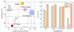
Figure 1: Comparison of different parameter-efficient tuning CIL baselines on CIFAR100 dataset. Left: The relationship between the average accuracy of the incremental sessions and the number of tunable parameters. Right: The average performance of old classes and new classes for each PET method.

Pre-trained vision transformer models [5] have demonstrated excellent performance on various vision tasks. Recently, it has been explored in the field of CIL and continues to receive considerable attention [50, 38, 37, 45]. Due to the powerful representation capabilities of pre-trained models, CIL methods based on pre-trained models achieve significant performance improvements compared to traditional SOTA methods which are trained from scratch. CIL with a pre-trained model typically fixes the pre-trained model to retain the generalizability and adds a few additional training parameters such as adapter [4], prompt [15] and SSF [22], which is referred to as parameter-efficient tuning (PET).

Inspired by language-based intelligence, current research in CIL is primarily focused on the prompt-based method [37, 31, 52]. Typically, these approaches require the construction of a pool of task-specific prompts during the training phase which increases storage overhead. Additionally, selecting prompts during the testing stage incurs additional computational costs. Other PET methods as well as fully fine-tuning are still in exploration in the context of CIL. Recently, SLCA [45] proposes fine-tuning the entire ViT and classifier incrementally with different learning rates. However, fine-tuning the entire pre-trained model requires substantial computational resources. In addition, Adam [50] initially explores the application of other PET methods in CIL using first-session adaptation and branch fusion. Training in the first stage and subsequently freezing the model can reduce training time but result in lower accuracy for subsequent new classes. Our linear probing results reveal that the first-session adaptation is insufficient when there is a significant domain discrepancy between downstream data and the pre-trained model.

In this paper, we first revisit different PET methods within the CIL paradigm. As shown in Fig. 1, we observe that adapter tuning [4] is a better continual learner than prompt-tuning [15] and SSF-tuning [22]. When progressively fine-tuning the prompt and SSF parameters, the forgetting of old classes is catastrophic. In comparison, adapter tuning effectively balances learning new classes and maintaining performance in old classes. Unlike prompt-based methods, which require constructing a prompt pool, adapter tuning avoids catastrophic forgetting even sharing the same parameters across learning sessions. Additionally, the adapter balances the number of tuning parameters and model performance compared to fully fine-tuning. Moreover, unlike previous methods that use feature distillation loss to restrict changes in shared parameters as part of overall loss, we analyze that tuning with constraints hinders continual learning from the perspective of parameter sensitivity. Therefore, we train the adapter and task-specific classifier without parameter regularization in each session, allowing for greater plasticity in learning new classes.

As we only train the local classifier in each learning session, we propose to adopt a new classifier retraining method [54, 45, 32] to further improve the CIL performance. First, we implicitly compute the semantic shift [42] of previous prototypes which leverages the semantic shift of current task samples to estimate the change of old classes. Then, we sample several features according to the updated prototypes to retrain the classifier which is more effective than previous methods. The advantages of our proposed method can be summarized as follows: 1) Fine-tuning adapters significantly reduces training costs and improves learning efficiency; 2) We do not need to retain any image samples; 3) The accuracy for new classes is relatively high which verifies the continual learning capacity of the model.

In summary, our proposed learning framework has the following main contributions: (1) Different from various devotion into the prompt-based methods for CIL, we discover that incrementally tuning adapter is a better continual learner even without constructing an adapter-pool; (2) After each session adaptation with local classifier, we propose to retrain a unified classifier with the semantic shift compensated prototypes which can further improve the performance; (3) Extensive experimental results on five CIL benchmarks demonstrate the superiority of the proposed simple but effective methods which achieves the SOTA.

2 Related Work

2.1 Class-incremental Learning

Class-incremental learning requires the model to be continuously updated with new class instances while retaining old knowledge [49]. Traditional CIL methods can be categorized into replay-based [2, 3, 28], regularization-based [17, 43, 40, 53], and parameter isolation-based methods [30, 23, 24]. Replay-based methods involve retaining or generating samples of previous classes and incorporating them into the current training phase. These methods often employ strategies for sample selection or sample generation to effectively replay past information. Regularization-based methods add constraints or penalties in the learning process which limit the update of the parameters that are important for old classes. Isolation-based methods aim to isolate and update task-specific parameters. By focusing on updating only a subset of parameters, these methods can mitigate catastrophic forgetting. To expand the representative capacity of a model without compromising its existing knowledge, methods for expanding the network have been proposed [41, 34, 48]. These methods dynamically extend the feature extraction network, combined with the replay-based method, achieving dramatic performance improvements.

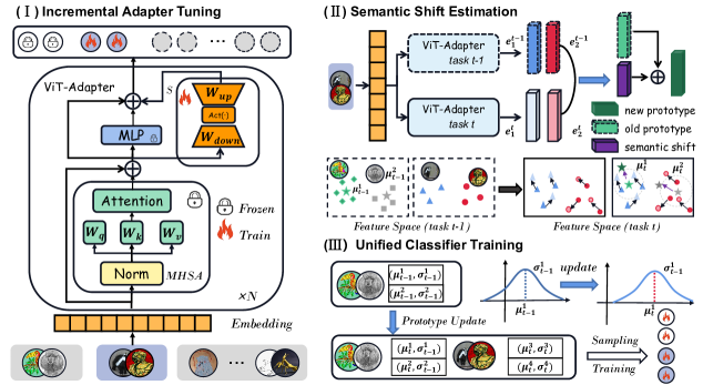
Figure 2: The framework of our proposed method. Left: The illustration of the structure of ViT and adapter. The adapter and local classifier are incrementally trained in each session using the Eq. 4. Right: The process of retraining the classifier with semantic shift estimation.

2.2 Parameter-Efficient Tuning

Parameter-Efficient Tuning can be considered as a transfer learning method. It refers to not performing full fine-tuning on a pre-trained model, instead inserting and fine-tuning specific sub-modules within the network. This approach is initially demonstrated to have effective transfer learning results in NLP [13, 19, 20, 14]. Recently, similar approaches have been applied to vision transformer models as well. AdaptFormer [4] inserts lightweight modules after the MLP layers in the attention module and has been found to outperform full fine-tuning on action recognition benchmarks. Another PET approach SSF [22] surprisingly outperforms other methods in certain tasks even with a smaller number of parameters. Inspired by the prompt approach used in the language model, VPT [15] applies it to visual models and achieves impressive results across various downstream tasks while only introducing a small number of additional parameters. Furthermore, the prompt-based method has also been used in vision-language models [27, 52, 51, 46] to improve performance on various downstream tasks.

2.3 Continual Learning on a Pre-trained Model

The aforementioned CIL methods all involve training the model from scratch, while CIL with pre-trained model [39, 52, 50, 35] has gained much attention due to its strong feature representation ability. L2P [52] utilizes the pre-trained model and learns a set of extra prompts dynamically to guide the model to solve corresponding tasks. DualPrompt [37] proposes to learn of two mutually unrelated prompt spaces: the general prompt and the expert prompt. It encodes task-invariant instructions and task-specific instructions, respectively. CODAPrompt [31] introduces a decomposed attention-based continual learning prompting method, which offers a larger learning capacity than existing prompt-based methods [52, 37]. SLCA [45] explores the fine-tuning paradigm of the pre-trained models, setting different learning rates for backbone and classifiers, and gains excellent performance. Adam [50] proposes to construct the classifier by merging the embeddings of a pre-trained model and an adapted downstream model. LAE [8] proposes a unified framework that calibrates the adaptation speed of tuning modules and ensembles PET modules to accomplish predictions.

3 Methodology

3.1 Preliminary

Class-incremental learning formulation: We first introduce the definition of CIL. Consider a neural network $\mathcal{M}_{\theta}=f_{\theta_{cls}}(\mathcal{F}_{\theta_{bne}}(\cdot))$ with trainable parameters $\theta=\{\theta_{bne},\theta_{cls}\}$. $\mathcal{F}_{\theta_{bne}}$ represents the feature extraction backbone which extracts features from input images and $f_{\theta_{cls}}$ stands for the classification layer that projects feature representations to class predictions. In CIL setting, $\mathcal{M}_{\theta}$ needs to learn a series of sessions from training data $D_{t}=\{(x^{t}_{1},y^{t}_{1}),(x^{t}_{2},y^{t}_{2}),...\},t=1,...,T$ and satisfy the condition $Y(i)\cap Y(j)=\emptyset,i\neq j$, where $Y(i)$ represent the label set in session $i$. The goal of $\mathcal{M}_{\theta}$ is to perform well on test sets that contain all the classes learned denoted as $\mathcal{Y}=Y(1)\cup...Y(t)$ after $t$-$th$ session.

Parameter-efficient tuning with Adapter: An adapter is a bottleneck structure [4] that can be incorporated into a pre-trained transformer-based network to facilitate transfer learning and enhance the performance of downstream tasks. An adapter typically consists of a downsampled MLP layer $W_{down}\in\mathbb{R}^{d\times\hat{d}}$, a non-linear activation function $\sigma$, and an upsampled MLP layer $W_{up}\in\mathbb{R}^{\hat{d}\times d}$. Denote the input as $x_{i}$, we formalize the adapter as

$$out=x_{i}+s\cdot\sigma(x_{i}*W_{down})*W_{up},\vspace{-2mm}$$ (1)

where $*$ stands for the matrix multiplication, $\sigma$ denotes the activation function RELU, and $s$ denotes the scale factor.

Parameter-efficient tuning with SSF: SSF [22] modulates pre-trained models using scale and shift factors to align the feature distribution of downstream tasks. SSF inserts its layers in each transformer operation. Suppose $x_{i}$ is the output of one of the modules, SSF can be represented as

$$y=\gamma\odot x_{i}+\beta,$$ (2)

where $\gamma\in\mathbb{R}^{d}$ and $\beta\in\mathbb{R}^{d}$ denote the scale and shift factor, respectively. $\odot$ stands for Hadamard product.

Parameter-efficient tuning with VPT: Visual Prompt Tuning (VPT) inserts a small number of trainable parameters in the input space after the embedding layer [15]. It is called prompts and only these parameters will be updated in the fine-tuning process. Depending on the number of layers inserted, VPT can be categorized as VPT-shallow and VPT-deep. Suppose $P=\{p^{k}\in R^{d}|1\leq k\leq n\}$ and the input embedding is $x$, VPT will combine $x$ with $P$ as

$$\vspace{-2mm}x^{\prime}=[x,P],$$ (3)

where $n$ is the number of prompts and the $x^{\prime}$ will be passed into subsequent blocks.

3.2 Adapter-tuning without parameter constraints

Most of the work based on pre-trained models focuses on how to apply the prompt-tuning strategies to the CIL paradigm. However, tuning the same prompt parameters across each learning session will cause catastrophic forgetting. As shown in Fig. 1, when progressively training the shared extra module while keeping the pre-trained model fixed, the adapter demonstrates its superiority over other tuning methods such as prompt-tuning and SSF. Fine-tuning the shared adapter incrementally seems to well balance the learning of new classes and old-knowledge retaining. Based on this observation, we delve deeper into incremental adapter tuning and use it as our baseline. The whole framework of the proposed method is shown in Fig. 2. Some methods [25, 47] adopt the first-session adaption and then fix the backbone. In addition, previous methods often utilize knowledge distillation [12] (KD) loss to restrict parameter changes of the feature extractor to mitigate forgetting. Totally different from earlier methods [21, 28, 17], we propose that the shared adapter should be tuned incrementally without parameter constraints. Next, we will provide a detailed description of the proposed baseline and offer a reasonable explanation and analysis.

Implementation of adapter-based baselines: During incremental training sessions, only adapter and classifier layers are updated, and the pre-trained ViT model is frozen. As the cosine classifier has shown great success in CIL, we follow ALICE [26] to use the cosine classifier with a margin. The margin hyper-parameter could also be used as a balance factor to decide the learning and retaining. The training loss can be formulated as follows:

$$\mathcal{L}^{t}=-\frac{1}{N^{t}}\sum_{j=1}^{N^{t}}log\frac{e^{s(cos\theta_{j}^{i}-m)}}{e^{s(cos\theta_{j}^{i}-m)}+\sum_{c=1}^{Y(t)-\{i\}}e^{s(cos\theta_{j}^{c})}}$$ (4)

where $cos\theta_{j}^{i}=\frac{w_{i}*f_{j}}{||w_{i}||*||f_{j}||}$, $N^{t}$ denotes the number of training samples of the current session, $s$ and $m$ represent the scale factor and margin factor, respectively.

As we do not retain any image samples, the gradients computed during the optimization of current samples not only affect the newly trained classifiers but also have an impact on the previously learned classifiers. The forgetting of the classifier is significant when no samples are retained. Thus, we follow previous work [45, 36, 8] to adopt the local training loss where we only compute the loss between current logits and labels and hinder the gradient updates of the previous classifier which alleviates the classifier forgetting.

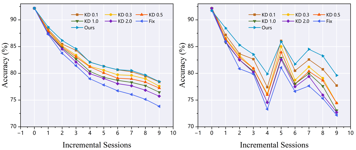
Figure 3: Comparison of the performance on ImageNetR dataset with different extent of parameter constraints. Left: The overall accuracy of each session. Right: The accuracy of new classes.

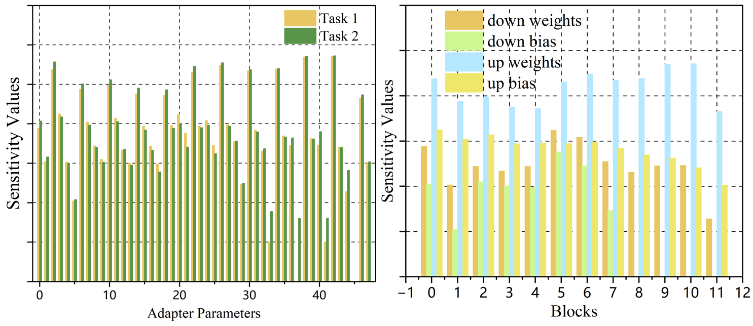
Figure 4: Parameter sensitivity analysis on the ImageNetR dataset. Left: The parameter sensitiveness of two incremental tasks. Right: The sensitiveness of different parameters in one task.

Analysis of the adapter-based baseline: We will analyze why the adapter shows its superiority in the CIL over other PET methods, and why we choose to incrementally tune the shared adapter without parameter constraints.

First, we elaborate on why incrementally tuning the adapter is better in the context of CIL. By utilizing the residual structure, the adapter can retain the generalization capabilities from the pre-trained model while adapting to new tasks. The incremental tuning of the adapter exhibits a cumulative learning capability, where the representational capacity of the adapter is further enhanced as the learning sessions progress. In contrast, both SSF and prompt tuning have limitations when it comes to handling CIL. These methods suffer from overfitting to the current distribution. When the shared parameters excessively overfit each current task, the model gradually loses its generalization ability which is harmful for training a unified model for CIL. Then, we try to utilize KD loss to implicitly limit parameter updates and adjust the weighting factor. As shown in Fig. 3, the results demonstrate that unconstrained training is more beneficial for new-classes learning and improving overall performance. Based on this observation, we propose our proposition from the perspective of parameter sensitivity.

Proposition 1: Confining the change of parameters of previous tasks hinders the plasticity of new classes due to the similarity of parameter sensitivity among tasks.

Proof: Given the parameter set $\theta=\{\theta_{1},\theta_{2},...\theta_{N}\}$ and training set $D_{t}=(X_{t},Y_{t})$ in $t$-$th$ session, the definition of parameter sensitivity [9, 47] is defined as

$$s_{i}^{t}=\mathcal{L}(X_{t},Y_{t}|\theta_{i})-\mathcal{L}(X_{t},Y_{t}|\theta_{i}^{*}),$$ (5)

where $\theta_{i}^{*}=\theta_{i}+\Delta\theta_{i}$ and $\mathcal{L}$ denotes the optimized loss in the classification task. We use the first-order Taylor expansion, and the parameter sensitivity can be rewritten as follows:

$$s_{i}=-g_{i}\Delta\theta_{i}=-\frac{\delta\mathcal{L}}{\delta\theta_{i}}*\Delta\theta_{i},$$ (6)

as $\Delta\theta_{i}$ denotes the update after the training process, we follow the work [9] to use the one-step update to approximate the $\Delta\theta_{i}=\epsilon\frac{\delta\mathcal{L}}{\delta\theta_{i}}$. Therefore, the parameter can be approximately computed as $s_{i}\approx-\epsilon(\frac{\delta\mathcal{L}}{\delta\theta_{i}})^{2}$. As shown in Fig. 4, the sensitivity values of tuning parameters for two different sessions are nearly equal and the most sensitive parameters are always up weights. This means that constraining the parameter update would hinder the learning of new classes and further impede the ability of the model for continual learning. Furthermore, in the experimental section, we demonstrate the representative capacity of the adapter continued to strengthen through incremental tuning.

3.3 Semantic shift estimation without past samples

Due to the selective updating of classifiers corresponding to the current task during training, the classifiers across different learning sessions are not fully aligned in the same feature space. To further optimize classifiers, we store the prototypes after training the backbone and local classifier. However, as the backbone is trained incrementally with new classes, the feature distribution of old classes undergoes changes. Retraining the classifier with the previous prototypes is sub-optimal. Since the feature representability of the backbone updates over time, using outdated features may not effectively retrain a unified classifier. To solve this problem, we update the feature distribution of old classes by computing the semantic shift over the learning process. We follow SDC [42] to estimate the semantic shift of old prototypes without access to past samples.

Suppose $\varphi_{c}^{t}$ denotes the prototype of category $c$ in session $t$ and $r$ is the learning session that the category belongs to. We have no access to the samples of category $c$ to update the prototype in session $t$ (when $t>r$). The semantic shift of class $c$ between two sessions can be represented as

$$\Delta_{c}^{r\rightarrow t}=\varphi_{c}^{t}-\varphi_{c}^{r},\quad\varphi_{c}^{r}=\frac{1}{N_{r}^{c}}\sum_{n=1}^{N_{r}^{c}}\mathcal{F}(X_{r}^{c},\theta_{r}).$$ (7)

While we do not have access to data from the old class $c$, we can only estimate the shift of current task categories on old and new models. The semantic shift of current samples between two sessions can be represented as

$$\delta_{i}^{t-1\to t}=e_{i}^{t}-e_{i}^{t-1},$$ (8)

where $e$ denotes the embedding of one sample in the current task $t$. We can compute $e_{i}^{t-1}$ at the start of the current task with the model trained in task $t-1$. After training on the new task, we compute $\delta_{i}^{t-1\to t}$ and use it to estimate $\Delta_{c}^{t-1\rightarrow t}$. We compute the shift as

$$\widetilde{\Delta}_{c}^{t-1\to t}= \frac{\sum\alpha_{i}\delta_{i}^{t-1\to t}}{\sum\alpha_{i}},c\notin C^{t},$$ (9)

$$\alpha_{i}= \mathbf{e}^{-\frac{||e_{i}^{t-1}-\varphi_{c}^{t-1}||}{2\sigma^{2}}},$$

where $\sigma$ is the standard deviation of the distribution of class $c$; $C^{t}$ denotes classes learned in the current session. Before retraining the classifier, we update the prototypes with

$$\left\{\begin{array}[]{lc}\varphi_{c}=\varphi_{c}^{t-1}+\widetilde{\Delta}_{c}^{t-1\to t}&,c\notin C^{t}\\ \varphi_{c}=\frac{1}{N_{c}}\sum_{i}e_{c}&,c\in C^{t},\\ \end{array}\right.$$ (10)

where $N_{c}$ denotes the number of images in class $c$.

3.4 Unified classifier training

Previous work [45, 32, 54] has attempted to retrain a unified classifier by modeling each class as a Gaussian distribution and sampling features from the distribution. We refer to this method as classifier alignment (CA) and adopt a similar approach that incorporates semantic shift estimation, which we denote as SSCA. Specifically, we compute the class prototypes $P_{c}=\{\varphi_{1},...,\varphi_{C}\}$ and covariance $\Sigma_{c}=\{\varsigma_{1},...,\varsigma_{C}\}$ for each class after training process in each learning session. The calculation of class prototypes is based on Eq. 10. Due to the capability of the trained backbone network to provide well-distributed representations, each class exhibits an unimodal distribution. Therefore, we form a normal distribution $\mathcal{N}(\mu_{c},\Sigma_{c})$ for each class with class prototype and variance. We sample features $\mathcal{V}_{c}=\{v_{c,1},...v_{c,S_{n}}\}$ from the distribution to obtain diverse samples, where $S_{n}$ is the number of the sample features for each class. Then, we use these features to train classification layers $\theta_{cls}$ with a commonly used cross-entropy loss as

$$\mathcal{L}(\theta_{cls},\mathcal{V}_{c})=-\sum_{i=1}^{S_{n}*C}log\frac{\mathbf{e}^{(\theta_{cls}^{j}(v_{i}))}}{\sum_{k\in C}\mathbf{e}^{(\theta_{cls}^{k}(v_{i}))}},\vspace{-1mm}$$ (11)

where $C$ denotes all classes learned so far. We normalize the features and classifier the same as backbone training.

Method	Params	Split-ImageNetR		Split-ImageNetA		CUB200		CIFAR100
		$\mathcal{A}_{Last}\uparrow$	$\mathcal{A}_{Avg}\uparrow$	$\mathcal{A}_{Last}\uparrow$	$\mathcal{A}_{Avg}\uparrow$	$\mathcal{A}_{Last}\uparrow$	$\mathcal{A}_{avg}\uparrow$	$\mathcal{A}_{Last}\uparrow$	$\mathcal{A}_{avg}\uparrow$
Joint	86M	$81.72_{\pm 0.35}$	-	$50.56_{\pm 1.75}$	-	$88.17_{\pm 0.32}$	-	$89.71_{\pm 0.07}$	-
FT	86M	$20.93_{\pm 0.86}$	$40.35_{\pm 0.74}$	$6.03_{\pm 4.74}$	$16.57_{\pm 5.8}$	$22.05_{\pm 1.69}$	$45.67_{\pm 2.04}$	$22.17_{\pm 1.09}$	$41.83_{\pm 1.60}$
SLCA [45]	86M	$79.35_{\pm 0.28}$	$83.29_{\pm 0.46}$	$61.05_{\pm 0.63}$	$68.88_{\pm 2.31}$	$84.68_{\pm 0.09}$	$90.77_{\pm 0.79}$	$91.26_{\pm 0.37}$	$94.29_{\pm 0.92}$
Adam-adapter [50]	1.19M	$65.79_{\pm 0.98}$	$72.42_{\pm 1.41}$	$48.81_{\pm 0.08}$	$58.84_{\pm 1.37}$	$85.84_{\pm 0.08}$	$91.33_{\pm 0.49}$	$87.29_{\pm 0.27}$	$91.21_{\pm 1.33}$
Adam-ssf [50]	0.2M	$66.61_{\pm 0.09}$	$74.36_{\pm 1.00}$	$48.94_{\pm 0.14}$	$58.79_{\pm 2.82}$	$85.67_{\pm 0.15}$	$90.99_{\pm 0.76}$	$85.27_{\pm 0.21}$	$89.90_{\pm 0.98}$
Adam-prompt [50]	0.04M	$65.29_{\pm 1.52}$	$72.97_{\pm 0.56}$	$29.29_{\pm 7.42}$	$39.14_{\pm 7.59}$	$85.28_{\pm 0.47}$	$90.89_{\pm 0.86}$	$85.04_{\pm 1.04}$	$89.49_{\pm 0.58}$
LAE [8]	0.19M	$72.29_{\pm 0.14}$	$77.99_{\pm 0.46}$	$47.18_{\pm 1.17}$	$58.15_{\pm 0.73}$	$80.97_{\pm 0.51}$	$87.22_{\pm 1.21}$	$85.25_{\pm 0.43}$	$89.80_{\pm 1.20}$
L2P [38]	0.04M	$72.34_{\pm 0.17}$	$77.36_{\pm 0.64}$	$44.04_{\pm 0.93}$	$51.24_{\pm 2.26}$	$67.02_{\pm 1.90}$	$79.62_{\pm 1.60}$	$84.06_{\pm 0.88}$	$88.26_{\pm 1.34}$
ADA [6]	1.19M	$73.76_{\pm 0.27}$	$79.57_{\pm 0.84}$	$50.16_{\pm 0.20}$	$59.43_{\pm 2.20}$	$76.13_{\pm 0.94}$	$85.74_{\pm 0.26}$	$88.25_{\pm 0.26}$	$91.85_{\pm 1.32}$
DualPrompt [37]	0.25M	$69.10_{\pm 0.62}$	$74.28_{\pm 0.66}$	$53.19_{\pm 0.74}$	$64.59_{\pm 0.08}$	$68.48_{\pm 0.47}$	$80.59_{\pm 1.50}$	$86.93_{\pm 0.24}$	$91.13_{\pm 0.32}$
CODAPrompt [31]	3.84M	$73.31_{\pm 0.50}$	$78.47_{\pm 0.53}$	$52.08_{\pm 0.12}$	$63.92_{\pm 0.12}$	$77.23_{\pm 1.12}$	$81.90_{\pm 0.85}$	$83.21_{\pm 3.39}$	$87.71_{\pm 3.17}$
SSIAT (Ours)	1.19M	$79.38_{\pm 0.59}$	$83.63_{\pm 0.43}$	$62.43_{\pm 1.63}$	$70.83_{\pm 1.63}$	$88.75_{\pm 0.38}$	$93.00_{\pm 0.90}$	$91.35_{\pm 0.26}$	$94.35_{\pm 0.60}$

Table 1: Experimental results on four CIL benchmarks. All other methods are reproduced using the same seeds for a fair comparison.

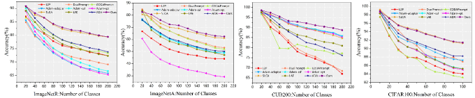
Figure 5: The performance of each learning session on four datasets. (a) ImageNetR; (b) ImageNetA; (c) CUB200; (d) CIFAR100. These curves are plotted by calculating the average performance across three different seeds for each incremental session.

4 Experiments

4.1 Datasets and Evaluation Protocols

Dataset: We evaluate our method on four commonly-used CIL benchmarks and one cross-domain CIL dataset. We randomly split the dataset into 10 or 20 learning tasks. CIFAR100 [18] is a widely used dataset in CIL which consists of 60000 images, belonging to 100 different categories. CUB200 [33] is a dataset that contains approximately 11,788 images of 200 bird species with fine-grained class labels. Additionally, we also follow recent work [50, 45] to use the other three datasets which have a large domain gap with pre-training data. ImageNetR [10] consists of 30,000 images with 200 categories. Although its categories overlap with ImageNet-21K [29], the images belong to a different domain. ImageNetA [11] is a real-world dataset that consists of 200 categories. This dataset exhibits significant class imbalance, with some categories having only a few training samples. VTAB [44] is a complex dataset that consists of 19 tasks covering a broad spectrum of domains and semantics. We follow previous work [50] to select 5 tasks to construct a cross-domain CIL dataset.

Method	ImageNetR		ImageNetA
	$\mathcal{A}_{Last}\uparrow$	$\mathcal{A}_{Avg}\uparrow$	$\mathcal{A}_{Last}\uparrow$	$\mathcal{A}_{Avg}\uparrow$
SLCA [45]	$74.63_{\pm 1.55}$	$79.92_{\pm 1.29}$	$36.69_{\pm 21.31}$	$56.35_{\pm 7.09}$
Adam-adapter[50]	$57.42_{\pm 0.84}$	$64.75_{\pm 0.79}$	$48.65_{\pm 0.12}$	$59.55_{\pm 1.07}$
Adam-ssf[50]	$64.30_{\pm 0.94}$	$72.42_{\pm 1.47}$	$47.27_{\pm 4.34}$	$58.36_{\pm 4.70}$
Adam-prompt[50]	$59.90_{\pm 1.13}$	$68.02_{\pm 1.02}$	$29.93_{\pm 4.88}$	$39.13_{\pm 4.19}$
LAE [8]	$69.86_{\pm 0.43}$	$77.38_{\pm 0.61}$	$39.52_{\pm 0.78}$	$51.75_{\pm 2.15}$
L2P [38]	$69.64_{\pm 0.42}$	$75.28_{\pm 0.57}$	$40.48_{\pm 1.78}$	$49.62_{\pm 1.46}$
DualPrompt [37]	$66.61_{\pm 0.58}$	$72.45_{\pm 0.37}$	$42.28_{\pm 1.94}$	$53.39_{\pm 1.64}$
CODAPrompt [31]	$69.96_{\pm 0.50}$	$75.34_{\pm 0.85}$	$44.62_{\pm 1.92}$	$54.86_{\pm 0.50}$
SSIAT (Ours)	$75.67_{\pm 0.14}$	$82.30_{\pm 0.36}$	$59.16_{\pm 1.03}$	$68.45_{\pm 1.92}$

Table 2: Experimental results for long-sequences (20 incremental sessions) on ImageNetR and ImageNetA dataset.

Implementation details: We use ViT-B/16 [5] as the pre-trained model, which is pre-trained on ImageNet-21K [29]. The initial learning rate is set as 0.01 and we use the cosine Anneal scheduler. In our experiments, we train the first session for 20 epochs and 10 epochs for later sessions. Following previous papers [50, 45], we use common evaluation metrics in CIL. Specifically, we report the last session accuracy $\mathcal{A}_{Last}$ and average accuracy of the whole incremental sessions $\mathcal{A}_{Avg}=\frac{1}{T}\sum_{i=1}^{T}\mathcal{A}_{i}$. We utilize three different seeds to generate three different class orders for evaluating various methods. We report the mean and standard deviation based on the three experiments. See codes.

4.2 Experiment Results

For a fair comparison, we compare our methods with SOTA CIL methods based on the pre-trained vision transformer model. We compare our methods with prompt-based methods L2P [52], DualPrompt [37], CODAPrompt [31], fine-tuning methods SLCA [45], and adapter-based method [50, 8, 6]. Tab. 1 shows $\mathcal{A}_{Avg}$ and $\mathcal{A}_{Last}$ with three different seeds on four CIL benchmarks.

CUB200 $\&$ CIFAR100: We first report the results of each method on the CUB200 and CIFAR100 datasets. Since these two datasets overlap with the pre-training data, methods based on a pre-trained model achieve a huge improvement in performance compared with methods that are trained from scratch. For example, as shown in Tab. 1, the average accuracy on L2P, DualPrompt, and CODAPrompt reached 88.26%, 91.13%, and 87.71% on CIFAR100, respectively. Nevertheless, our method still outperforms those prompt-based methods. Besides, our method does not require the construction of a prompt pool which allows each task to learn specific prompt parameters. The adapter is shared across tasks and our method avoids the parameter expansion with tasks increasing. Even though the Adam-adapter/SSF/prompt only needs to train in the first stage which requires less training time, the performance of those methods is inferior to our proposed method. Although the performance of SLCA is comparable to our method in CIFAR100, the number of tuning parameters of our method is much smaller. Besides that, the average performance of our method on CUB200 is 93.00$\%$, nearly 2.3$\%$ improvement over SLCA. Fig. 5 (c) (d) shows the incremental accuracy of each session on CUB200 and CIFAR100 and our method is always at the top of all lines in the incremental process.

Method	Ses.1	Ses.2	Ses.3	Ses.4	Ses.5	Avg$\uparrow$
Adam-adapter[50]	87.60	86.07	89.14	82.72	84.35	85.97
Adam-ssf[50]	89.60	88.21	89.94	80.50	82.38	86.13
Adam-vpt[50]	90.20	87.57	89.69	80.39	82.18	86.01
SLCA[45]	94.80	92.43	93.54	93.98	94.33	93.82
LAE [8]	97.99	85.26	79.68	78.78	74.36	83.21
SSIAT (Ours)	96.10	92.71	94.09	93.68	94.50	94.21

Table 3: Experimental results for different methods on VTAB dataset which contain 5 datasets from different domains.

PET Method	Params	Ses.1	Ses.2	Ses.3	Ses.4	Ses.5	Ses.6	Ses.7	Ses.8	Ses.9	Ses.10	Avg$\uparrow$
SSF [22]	0.2M	98.50	91.90	88.57	85.02	83.92	78.70	77.79	77.89	73.02	74.91	83.03
VPT-deep [15]	0.046M	97.60	69.15	68.70	56.60	55.56	48.87	55.97	56.05	53.48	55.21	61.72
VPT-shallow [15]	0.004M	98.40	92.95	88.80	92.06	87.26	86.37	85.64	85.31	85.36	85.10	88.72
Adapter [4]	1.19M	98.50	95.35	91.60	91.08	90.92	90.08	89.80	89.62	88.98	89.29	91.52

Table 4: Experimental results for baselines with different efficient tuning methods on CIFAR100. We report the overall performance of each session and the average performance.

ImageNetR $\&$ ImageNetA: We report the performance on ImageNetR and ImageNetA in Tab. 1. These two datasets are more difficult due to the domain gap with the pre-training data. It can be seen that the performance of each method on these two datasets is lower than CIFAR100 and CUB200. Besides, we can see that SLCA outperforms other previous methods significantly on these two datasets. Notably, SLCA achieves an impressive last accuracy on ImageNetR, surpassing the other methods. In contrast, our method achieves SOTA-level performance on both datasets with fewer tuning parameters. Based on Fig. 5, the performance of our method is slightly higher than SLCA in several learning sessions with fewer tuning parameters on the ImageNetR dataset. On the ImageNetA dataset, our method achieves the last accuracy of 62.43%, surpassing SLCA by 1.39%. The average accuracy across all sessions is 70.83%, showing a 2% improvement.

Additionally, we evaluate the performance of each method under the condition of long sequences. In this setting, each session consists of only 10 classes, and the results are summarized in Tab. 2. Our method also maintains excellent performance in terms of $\mathcal{A}_{Last}$ and $\mathcal{A}_{Avg}$. The performance of SLCA is highly dependent on the class order in which the training data appears, resulting in a substantial variance in $\mathcal{A}_{Last}$ on ImageNetA. In contrast, the Adam-based methods remain relatively stable in long-sequence settings. For Adam-SSF, the long sequence only leads to a nearly $2\%$ performance drop in ImageNetR. However, for SLCA, its performance drops by $5\%$ on ImageNetR and nearly $10\%$ on ImageNetA. In comparison, our method demonstrates excellent stability on long sequences and outperforms other methods by a large margin.

Classifier	Method	Ses.1	Ses.2	Ses.3	Ses.4	Ses.5	Ses.6	Ses.7	Ses.8	Ses.9	Ses.10	Avg$\uparrow$
Linear	w/o CA	74.65	68.37	63.90	58.82	58.02	55.48	54.03	52.89	51.62	52.13	58.99
	w/ CA	74.65	71.59	67.93	64.24	62.08	60.90	59.03	57.32	56.41	56.85	63.10
	w/ SSCA	74.65	70.92	67.64	63.91	62.65	60.96	60.38	58.55	58.13	57.77	63.55
Cosine	w/o CA	82.66	77.78	72.20	67.63	66.01	63.18	59.97	59.35	58.93	57.91	66.56
	w/ CA	82.66	79.70	74.56	70.40	68.19	65.66	63.40	61.77	60.70	59.78	68.68
	w/ SSCA	82.66	80.60	75.91	72.41	71.56	69.01	66.10	64.60	63.00	62.43	70.83

Table 5: Ablation results for unified classifier training and semantic shift estimation on ImageNetA. We report the overall performance of each session and the average performance. We run the experiments with three seeds and reported the average performance.

Method	CIFAR	ImageNetR	ImageNetA	CUB
No-Adapt.	86.08	68.42	33.71	86.77
First-Adapt.	91.33	78.02	63.53	89.27
All-Adapt.	92.57	82.02	65.96	89.86
$\Delta\uparrow$	$1.24\%$	$4.00\%$	$2.43\%$	$0.59\%$

Table 6: Linear probing results of different training ways on four datasets. We retrain the classifier using all the data on the fixed-trained backbone.

Structure	Params	CIFAR	ImageNetR	ImageNetA
AdaptMLP-P [4]	1.19M	$94.35_{\pm 0.60}$	$83.63_{\pm 0.43}$	$70.83_{\pm 1.63}$
AdaptMLP-S [4]	1.19M	$94.16_{\pm 0.88}$	$83.19_{\pm 0.47}$	$71.00_{\pm 1.52}$
Convpass [16]	1.63M	$94.08_{\pm 0.99}$	$83.64_{\pm 0.35}$	$69.96_{\pm 1.09}$
Adapter [13]	2.38M	$94.26_{\pm 0.91}$	$83.65_{\pm 0.50}$	$70.94_{\pm 1.42}$

Table 7: Experimental results of different adapter structures. We report the average performance and standard deviation.

VTAB: VTAB is a cross-domain CIL dataset where each task provides training data from a different domain. Based on the results presented in Tab. 3, it can be observed that both SLCA and our method perform well in cross-domain CIL. Specifically, in the last incremental stage, our method achieves an accuracy that is $12\%$ higher than the Adam-based methods. Adam-based methods only perform fine-tuning in the first task and are not able to adapt well to subsequent tasks on the cross-domain dataset.

4.3 Ablation Study

Baselines with different PET methods: Tab. 4 shows the results of baselines with three different parameter-efficient tuning methods in each incremental session. It can be observed that the pre-trained model with an adapter achieves the best performance in terms of both the last session accuracy and average accuracy. Fig. 1 demonstrates that tuning with an adapter achieves a better balance between learning new classes and retaining knowledge of old classes. Both VPT-deep and SSF methods tend to prioritize learning new categories, which leads to increased forgetting of previously learned categories. Although VPT-shallow performs well on CIFAR, its limited parameters hinder the model from incrementally learning new classes on ImageNetR. More results on the other datasets can be found in the Supp.

Unified classifier retraining vs. Separate local classifier: As we train separate task-specific classifiers in each incremental session, we propose to retrain the classifier to find the optimal decision boundary for all the classes. Tab. 5 displays the ablation experiments of the classifier re-trained on ImageNetA which is the most difficult benchmark. It can be observed that whether it is a linear or a cosine classifier, retraining the classifier leads to a significant performance improvement. Additionally, incorporating the computation of prototype semantic shifts further enhances the performance by an additional $2\%$ in the cosine classifier. Compared to the classifier alignment methods that do not involve computing updated prototypes, our method demonstrates its superiority as the incremental stages progress. More results on the other datasets can be found in the Supp.

Progressively tuning vs. first session adaptation: Tab. 6 shows the linear probing results of different adaption ways. After finishing the training of the last session, we freeze the pre-trained backbone and only train the classifier using all the samples. It is evident that not performing tuning and solely freezing the pre-trained model leads to the worst performance, regardless of the dataset. First-session adaptation proves to be a good choice as it reduces training time and works well for datasets like CIFAR100 and CUB200. However, for datasets such as ImageNetA and ImageNetR, which have significant domain gaps from the pre-trained model, relying solely on first-session adaptation is suboptimal. By continuously fine-tuning the adapter, we observe that the backbone exhibits stronger representability compared to only tuning in the first session.

Different structures of the adapter: In this paper, we follow AdaptFormer [4] to use parallel adapterMLP as the adapter structure. We also delve deeper into different adapter structures such as Adapter [13] and Convpass [16]. Although these different tuning structures may exhibit performance differences under static settings, the performance differences among those adapter structures are minimal in the context of CIL shown in Tab. 7. This offers us the flexibility to employ various adapter structures within the context of the CIL paradigm.

Comparison to traditional CIL methods: We conduct evaluations by comparing our approach to SOTA traditional CIL methods shown in Tab. 8. We replace the Resnet backbone with the pre-trained ViT model for fair comparison. The results indicate that the performance of iCaRL tends to be inferior compared to SOTA model expansion methods and our proposed method, even when past samples are stored. It can be observed that methods such as Foster and Der, which dynamically expand feature extraction networks, achieve impressive results on ImageNetR. The average accuracy of these methods is only $2\%$ lower than our method. However, on ImageNetA, where there are few-shot samples for many classes, these methods exhibit low performance. More ablation experiments related to hyper-parameters can be found in the supp.

Method	ImageNetR		ImageNetA
	$\mathcal{A}_{Last}\uparrow$	$\mathcal{A}_{Avg}\uparrow$	$\mathcal{A}_{Last}\uparrow$	$\mathcal{A}_{Avg}\uparrow$
iCaRL [28]	$61.70_{\pm 0.56}$	$71.34_{\pm 0.67}$	$29.32_{\pm 2.36}$	$40.11_{\pm 1.36}$
Foster [34]	$75.87_{\pm 0.38}$	$81.54_{\pm 0.82}$	$12.44_{\pm 17.45}$	$17.01_{\pm 20.44}$
Der [41]	$75.63_{\pm 0.86}$	$81.13_{\pm 0.11}$	$38.43_{\pm 2.39}$	$46.43_{\pm 3.29}$
Memo [48]	$65.38_{\pm 0.90}$	$73.80_{\pm 0.86}$	$28.45_{\pm 2.37}$	$40.27_{\pm 1.22}$
SSIAT (Ours)	$79.38_{\pm 0.59}$	$83.63_{\pm 0.43}$	$62.43_{\pm 1.63}$	$70.83_{\pm 1.63}$

Table 8: Comparison to traditional CIL methods on ImageNetR and ImageNetA dataset.

5 Conclusion

Class-incremental learning on a pre-trained model has received significant attention in recent years. In this paper, we first revisit different PET methods in the context of CIL. Then, we propose that incrementally tuning the shared adapter and local classifier without constraints exhibits less forgetting and gains plasticity for learning new classes. Moreover, to train a unified classifier, we calculate the semantic shift of old prototypes and retrain the classifier using updated prototypes in each session. The proposed method eliminates the need for constructing an adapter pool and avoids retaining any image samples. Experimental results on five benchmarks demonstrate the effectiveness of our method which achieves the SOTA performance.

Acknowledgement. This research was supported by Natural Science Fund of Hubei Province (Grant # 2022CFB823), Alibaba Innovation Research program under Grant Contract # CRAQ7WHZ11220001-20978282, and HUST Independent Innovation Research Fund (Grant # 2021XXJS096).

Appendix

A. More experiments on parameter sensitivity

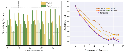
Figure 6: left: Parameter sensitivity of the different modules of task 2 and task 3. right: Incremental performance of varying degrees of update limits on important parameters.

We conduct parameter sensitivity experiments on ImageNetR, and the results are shown in Fig. 6. The left graph illustrates the parameter sensitivity of the second and third tasks. Similar to the trends observed in task one and two as shown in the main paper, the parameter sensitivity of different modules in task two and three also exhibits a high degree of similarity. Therefore, restricting parameter updates based on parameter sensitivity negatively impacts the learning of new categories. To investigate this phenomenon, we conduct experiments, as shown in the right graph. It can be seen that as the restriction on parameter updates in increases, the overall performance decreases.

B. More Ablation Experiments

Adapter dimension and layers insert: As shown in Tab. 9 and 10 left, we further conduct experiments on the specific position to insert the adapter module on the ImageNetR and ImageNetA datasets. We observe that the performance is progressively improved with the number of layers increased. Thus, we insert adapter modules in all $12$ layers in our comparative experiments of various methods. We also conduct ablation experiments on the middle dimension in the adapter in Tab. 9 and 10 right. We observe that increasing the dimension has a positive effect on the performance of the model. Interestingly, setting the middle dimension to 32 did not result in a significant decrease in performance. On the other hand, setting it to 256 led to an improvement in performance but also quadrupled the number of parameters. To strike a balance between performance and the number of fine-tuning parameters, we set the middle dimension to $64$.

Analysis of margin and scale: We conduct experiments on the hyper-parameter of the scale and margin in our cosine loss as shown in Tab. 13. We discover that appropriately increasing scale can enhance the performance of the model. For example, on the ImageNetR dataset, when the scale is set to $20$, the average accuracy is $3.36\%$ higher than when the value is $10$. We also conduct experiments to analyze the influence of the margin. As shown in Tab. 14, we observe that different datasets have different appropriate margin values. For example, on the ImageNetR dataset, we set the margin to $0.0$, and on the CUB200 dataset, we set it to $0.1$.

Layers	Form	Acc	Num	#Param	Acc
1-3	parallel	80.53	32	0.60M	81.98
1-6	parallel	81.63	64	1.19M	82.09
1-12	parallel	81.95	256	4.87M	82.38

Table 9: Experimental results of the inserted layers of the adapter and the middle dimension.

Different PET methods in the CIL: The experiment results on CIFAR100 are in the main paper. In the supplementary material, we provide experiments with different PET methods on ImageNetR as shown in Tab. 15. We can observe that in the initial sessions, the performance of SSF surpasses that of the adapter. However, due to the tendency of SSF to overfit to the current session classes, there is a significant decline in subsequent incremental sessions and the adapter performs best in both the accuracy of the last session and average accuracy. We also provide experiments on ImageNetA as shown in Tab. 16. We can draw the same conclusion from ImageNetR.

Layers	Form	Acc	Num	#Param	Acc
1-3	parallel	65.25	32	0.60M	66.49
1-6	parallel	65.81	64	1.19M	66.85
1-12	parallel	66.67	256	4.87M	67.54

Table 10: Experimental results of the inserted layers of the adapter and the middle dimension.

Unified classifier retraining vs. Separate local classifier: The experiment results on ImageNetA are in the main paper. Here we show the accuracy of each session of three different seeds on ImageNetA as shown in Tab. 17. It can be seen that retraining the classifier can improve the performance by $2\%$ to $3\%$ on three seeds, effectively improving the performance of the classifier. Furthermore, classifier retraining with semantic shift estimation can further improve performance by $2\%$ to $3\%$. We also show the results on CUB200 as shown in Tab. 18. The same trend is shown in this dataset. CA can significantly improve the performance, and SSCA can align the prototype and further improve performance. The results on ImageNetR are shown in Tab. 19.

Different pre-trained models. We experiment with pre-trained models (PTMs) with different generalization abilities on ImageNetR and ImageNetA datasets shown in Tab. 11. It can be observed that our method generalizes well to various PTMs. The large-based ViT model can get better performance.

Different tuning methods with SSCA. We incorporate classifier alignment with semantic shift estimation into SSF and prompt tuning shown in Tab. 12. It can be seen that both the performance of prompt-based and SSF tuning approaches show significant improvement. However, our proposed method still outperforms them by a large margin. The results further verify the effectiveness of our proposed method.

Pre-trained Model	ImageNetR		ImageNetA
	$\mathcal{A}_{Last}\uparrow$	$\mathcal{A}_{Avg}\uparrow$	$\mathcal{A}_{Last}\uparrow$	$\mathcal{A}_{Avg}\uparrow$
ViT-base 1K	$80.15_{\pm 0.41}$	$83.87_{\pm 0.26}$	$64.88_{\pm 1.11}$	$72.68_{\pm 1.72}$
ViT-base 21k	$79.38_{\pm 0.59}$	$83.63_{\pm 0.43}$	$62.43_{\pm 1.63}$	$70.83_{\pm 1.63}$
ViT-large 21k	$83.62_{\pm 0.41}$	$86.70_{\pm 0.69}$	$68.38_{\pm 2.25}$	$74.85_{\pm 1.93}$

Table 11: Results on different pre-trained models on ImageNetR/A.

Method	ImageNetR		ImageNetA
	$\mathcal{A}_{Last}\uparrow$	$\mathcal{A}_{Avg}\uparrow$	$\mathcal{A}_{Last}\uparrow$	$\mathcal{A}_{Avg}\uparrow$
SSF	$71.84_{\pm 0.33}$	$79.98_{\pm 0.79}$	$52.11_{\pm 0.64}$	$62.34_{\pm 1.33}$
+SSCA	$75.01_{\pm 0.31}$	$82.09_{\pm 0.41}$	$58.94_{\pm 1.09}$	$67.94_{\pm 1.06}$
VPT-deep	$38.49_{\pm 0.13}$	$50.34_{\pm 1.93}$	$37.39_{\pm 22.03}$	$46.55_{\pm 16.69}$
+SSCA	$56.11_{\pm 3.25}$	$61.11_{\pm 1.71}$	$47.83_{\pm 18.75}$	$55.67_{\pm 14.92}$
VPT-shallow	$58.79_{\pm 1.07}$	$69.23_{\pm 4.06}$	$48.34_{\pm 0.99}$	$56.96_{\pm 3.45}$
+SSCA	$68.25_{\pm 2.50}$	$72.40_{\pm 2.23}$	$54.49_{\pm 0.76}$	$62.26_{\pm 2.54}$

Table 12: Results for different PET methods on ImageNetR/A.

Scale	ImageNetR		ImageNetA		CIFAR100		CUB200
	Last $\uparrow$	Avg $\uparrow$	Last $\uparrow$	Avg $\uparrow$	Last $\uparrow$	Avg $\uparrow$	Last $\uparrow$	Avg $\uparrow$
s=10	73.80	80.84	56.95	66.88	89.49	93.61	86.39	91.61
s=15	77.83	83.36	59.84	69.25	91.02	94.53	88.46	92.57
s=20	79.55	84.20	60.76	69.62	91.62	94.75	88.51	92.83
s=30	78.90	83.30	60.50	68.73	91.21	94.51	88.60	92.64

Table 13: Experimental results of the influence of scale in cosine loss on different datasets.

Margin	ImageNetR		ImageNetA		CIFAR100		CUB200
	Last$\uparrow$	Avg $\uparrow$	Last $\uparrow$	Avg $\uparrow$	Last $\uparrow$	Avg $\uparrow$	Last $\uparrow$	Avg $\uparrow$
m = 0	79.55	84.20	60.76	69.62	91.62	94.75	88.13	92.33
m = 0.1	78.38	84.25	63.00	72.13	91.60	94.71	88.46	92.57
m = 0.2	76.48	82.94	62.74	73.18	89.71	93.28	88.38	92.56
m = 0.3	73.90	80.76	62.61	72.46	86.83	91.45	87.57	91.89

Table 14: Experimental results of the influence of margin in cosine loss on different datasets.

PET Method	Params	Ses.1	Ses.2	Ses.3	Ses.4	Ses.5	Ses.6	Ses.7	Ses.8	Ses.9	Ses.10	Avg$\uparrow$
SSF [22]	0.2M	94.75	89.28	86.11	82.61	80.19	78.67	77.27	75.4	75.04	72.78	81.21
VPT-deep [15]	0.046M	87.23	64.19	59.16	40.27	39.4	36.6	31.51	33.32	33.79	31.62	45.71
VPT-shallow [15]	0.004M	81.86	73.20	68.81	66.85	64.89	63.81	62.84	62.21	61.35	58.97	66.48
Adapter [4]	1.19M	91.87	88.42	86.51	84.43	82.75	81.51	80.99	80.62	79.75	78.28	83.51

Table 15: Experimental results for baselines with different parameter efficient tuning methods on ImageNetR. We report the overall performance of each session and the average performance.

PET Method	Params	Ses.1	Ses.2	Ses.3	Ses.4	Ses.5	Ses.6	Ses.7	Ses.8	Ses.9	Ses.10	Avg$\uparrow$
SSF [22]	0.2M	82.86	76.11	67.44	65.62	61.47	58.97	54.33	52.32	51.04	51.28	62.14
VPT-deep [15]	0.046M	61.14	31.67	15.55	15.62	10.11	6.05	4.82	4.17	3.37	3.42	15.92
VPT-shallow [15]	0.004M	80.00	70.00	64.92	60.32	56.84	54.26	52.63	51.52	49.68	48.26	58.84
Adapter	1.19M	82.86	74.72	71.43	67.62	64.68	62.15	59.14	56.89	55.20	55.50	65.02

Table 16: Experimental results for baselines with different parameter efficient tuning methods on ImageNetA. We report the overall performance of each session and the average performance.

Seed	Method	Ses.1	Ses.2	Ses.3	Ses.4	Ses.5	Ses.6	Ses.7	Ses.8	Ses.9	Ses.10	Avg $\uparrow$
1993	w/o CA	85.71	81.11	75.84	72.92	68.85	64.21	60.48	60.18	59.07	58.66	68.70
	w/ CA	85.71	81.94	77.10	73.07	71.22	68.00	64.14	63.22	60.14	59.91	70.45
	w/ SSCA	85.71	83.61	78.57	76.36	73.84	72.00	66.73	65.06	62.37	62.15	72.64
1996	w/o CA	81.99	77.34	71.36	64.74	66.14	63.83	62.54	60.25	60.09	58.39	66.67
	w/ CA	81.99	78.06	74.57	67.91	67.15	64.57	64.59	62.62	61.92	62.08	68.55
	w/ SSCA	81.99	78.06	74.81	69.78	71.18	67.9	66.43	65	64.2	64.19	70.35
1997	w/o CA	80.29	74.91	69.41	65.23	63.03	61.49	56.89	57.63	57.62	56.68	64.32
	w/ CA	80.29	79.09	72	70.22	66.21	64.41	61.46	59.46	60.03	57.34	67.05
	w/ SSCA	80.29	80.14	74.35	71.08	69.66	67.12	65.15	63.73	62.44	60.96	69.49

Table 17: Ablation results for unified classifier training and semantic shift estimation on ImageNetA. We report the overall performance of each session and the average performance.

Seed	Method	Ses.1	Ses.2	Ses.3	Ses.4	Ses.5	Ses.6	Ses.7	Ses.8	Ses.9	Ses.10	Avg $\uparrow$
1993	w/o CA	99.19	95.37	91.37	87.81	85.86	82.49	82.15	80.96	79.09	78.63	86.29
	w/ CA	99.19	98.24	93.45	91.62	91.33	88.42	87.69	86.78	86.37	85.50	90.86
	w/ SSCA	99.19	98.24	94.64	93.14	93.10	91.45	90.68	90.59	89.71	88.80	92.95
1996	w/o CA	100.00	94.79	91.09	90.02	88.34	85.92	85.59	82.74	80.87	79.05	87.84
	w/ CA	100.00	95.83	94.60	92.60	92.00	90.83	90.56	86.84	85.40	85.58	91.42
	w/ SSCA	100.00	96.25	96.06	94.96	94.30	93.81	93.32	91.26	90.22	89.10	93.93
1997	w/o CA	96.55	97.20	91.9	87.87	84.92	84.28	82.15	82.1	82.69	78.92	86.86
	w/ CA	96.55	97.90	95.8	90.67	90.12	90.29	87.96	87.43	86.98	85.88	90.96
	w/ SSCA	96.55	97.67	95.8	92.02	91.25	91.30	89.56	89.5	89.39	88.34	92.14

Table 18: Ablation results for unified classifier training and semantic shift estimation on CUB200. We report the overall performance of each session and the average performance.

Seed	Method	Ses.1	Ses.2	Ses.3	Ses.4	Ses.5	Ses.6	Ses.7	Ses.8	Ses.9	Ses.10	Avg $\uparrow$
1993	w/o CA	91.73	88.64	86.14	84.59	82.08	81.32	80.68	80.52	79.67	78.47	83.38
	w/ CA	91.73	88.12	86.20	84.51	82.08	81.26	81.32	81.00	79.38	78.02	83.36
	w/ SSCA	91.73	88.57	86.72	84.95	82.91	82.19	82.32	81.63	80.43	79.58	84.10
1996	w/o CA	89.55	86.63	85.27	82.45	81.64	80.36	79.56	78.33	78.34	77.40	81.95
	w/ CA	89.55	87.59	86.37	83.58	82.15	81.12	79.85	78.81	78.51	77.67	82.52
	w/ SSCA	89.55	87.11	86.65	84.04	83.34	82.00	81.51	79.87	79.73	78.72	83.25
1997	w/o CA	91.20	87.90	85.17	82.96	80.57	80.59	79.35	78.14	77.85	77.68	82.14
	w/ CA	91.20	88.73	85.52	83.47	81.88	81.02	79.70	79.06	78.42	78.40	82.74
	w/ SSCA	91.20	89.00	86.16	83.68	82.40	81.75	80.97	80.63	79.73	79.85	83.54

Table 19: Ablation results for unified classifier training and semantic shift estimation on ImageNetR. We report the overall performance of each session and the average performance.

C. More Implementation Details

To mitigate the impact of randomness in the experiments, we selected three different seeds (1993,1996, and 1997) to conduct experiments separately and calculate the average and variance. In experiments involving different PET methods, we fine-tuned the parameters inserted into the network without unified classifier retraining. For experiments of adapter dimension and layers insert, we conduct experiments on the ImageNetR dataset and we set the loss margin to $0.0$ and the scale to $20$. In the analysis of margin experiments, we set the scale to $20$ for all datasets. In the analysis of scale experiments, we set the scale to $0.0$ for all datasets.

References

- Aljundi et al. [2018] Rahaf Aljundi, Francesca Babiloni, Mohamed Elhoseiny, Marcus Rohrbach, and Tinne Tuytelaars. Memory aware synapses: Learning what (not) to forget. In Proceedings of the European conference on computer vision (ECCV), pages 139–154, 2018.
- Bang et al. [2021] Jihwan Bang, Heesu Kim, YoungJoon Yoo, Jung-Woo Ha, and Jonghyun Choi. Rainbow memory: Continual learning with a memory of diverse samples. In Proceedings of the IEEE/CVF conference on computer vision and pattern recognition, pages 8218–8227, 2021.
- Chaudhry et al. [2018] Arslan Chaudhry, Puneet K Dokania, Thalaiyasingam Ajanthan, and Philip HS Torr. Riemannian walk for incremental learning: Understanding forgetting and intransigence. In Proceedings of the European conference on computer vision (ECCV), pages 532–547, 2018.
- Chen et al. [2022] Shoufa Chen, Chongjian Ge, Zhan Tong, Jiangliu Wang, Yibing Song, Jue Wang, and Ping Luo. Adaptformer: Adapting vision transformers for scalable visual recognition. Advances in Neural Information Processing Systems, 35:16664–16678, 2022.
- Dosovitskiy et al. [2020] Alexey Dosovitskiy, Lucas Beyer, Alexander Kolesnikov, Dirk Weissenborn, Xiaohua Zhai, Thomas Unterthiner, Mostafa Dehghani, Matthias Minderer, Georg Heigold, Sylvain Gelly, et al. An image is worth 16x16 words: Transformers for image recognition at scale. arXiv preprint arXiv:2010.11929, 2020.
- Ermis et al. [2022] Beyza Ermis, Giovanni Zappella, Martin Wistuba, Aditya Rawal, and Cedric Archambeau. Memory efficient continual learning with transformers. Advances in Neural Information Processing Systems, 35:10629–10642, 2022.
- French [1999] Robert M French. Catastrophic forgetting in connectionist networks. Trends in cognitive sciences, 3(4):128–135, 1999.
- Gao et al. [2023] Qiankun Gao, Chen Zhao, Yifan Sun, Teng Xi, Gang Zhang, Bernard Ghanem, and Jian Zhang. A unified continual learning framework with general parameter-efficient tuning. arXiv preprint arXiv:2303.10070, 2023.
- He et al. [2023] Haoyu He, Jianfei Cai, Jing Zhang, Dacheng Tao, and Bohan Zhuang. Sensitivity-aware visual parameter-efficient tuning. arXiv preprint arXiv:2303.08566, 2023.
- Hendrycks et al. [2021a] Dan Hendrycks, Steven Basart, Norman Mu, Saurav Kadavath, Frank Wang, Evan Dorundo, Rahul Desai, Tyler Zhu, Samyak Parajuli, Mike Guo, et al. The many faces of robustness: A critical analysis of out-of-distribution generalization. In Proceedings of the IEEE/CVF International Conference on Computer Vision, pages 8340–8349, 2021a.
- Hendrycks et al. [2021b] Dan Hendrycks, Kevin Zhao, Steven Basart, Jacob Steinhardt, and Dawn Song. Natural adversarial examples. In Proceedings of the IEEE/CVF Conference on Computer Vision and Pattern Recognition, pages 15262–15271, 2021b.
- Hinton et al. [2015] Geoffrey Hinton, Oriol Vinyals, and Jeff Dean. Distilling the knowledge in a neural network. arXiv preprint arXiv:1503.02531, 2015.
- Houlsby et al. [2019] Neil Houlsby, Andrei Giurgiu, Stanislaw Jastrzebski, Bruna Morrone, Quentin De Laroussilhe, Andrea Gesmundo, Mona Attariyan, and Sylvain Gelly. Parameter-efficient transfer learning for nlp. In International Conference on Machine Learning, pages 2790–2799. PMLR, 2019.
- Hu et al. [2021] Edward J Hu, Yelong Shen, Phillip Wallis, Zeyuan Allen-Zhu, Yuanzhi Li, Shean Wang, Lu Wang, and Weizhu Chen. Lora: Low-rank adaptation of large language models. arXiv preprint arXiv:2106.09685, 2021.
- Jia et al. [2022] Menglin Jia, Luming Tang, Bor-Chun Chen, Claire Cardie, Serge Belongie, Bharath Hariharan, and Ser-Nam Lim. Visual prompt tuning. In European Conference on Computer Vision, pages 709–727. Springer, 2022.
- Jie and Deng [2022] Shibo Jie and Zhi-Hong Deng. Convolutional bypasses are better vision transformer adapters. arXiv preprint arXiv:2207.07039, 2022.
- Kirkpatrick et al. [2017] James Kirkpatrick, Razvan Pascanu, Neil Rabinowitz, Joel Veness, Guillaume Desjardins, Andrei A Rusu, Kieran Milan, John Quan, Tiago Ramalho, Agnieszka Grabska-Barwinska, et al. Overcoming catastrophic forgetting in neural networks. Proceedings of the national academy of sciences, 114(13):3521–3526, 2017.
- Krizhevsky et al. [2009] Alex Krizhevsky, Geoffrey Hinton, et al. Learning multiple layers of features from tiny images. 2009.
- Lester et al. [2021] Brian Lester, Rami Al-Rfou, and Noah Constant. The power of scale for parameter-efficient prompt tuning. arXiv preprint arXiv:2104.08691, 2021.
- Li and Liang [2021] Xiang Lisa Li and Percy Liang. Prefix-tuning: Optimizing continuous prompts for generation. arXiv preprint arXiv:2101.00190, 2021.
- Li and Hoiem [2017] Zhizhong Li and Derek Hoiem. Learning without forgetting. IEEE transactions on pattern analysis and machine intelligence, 40(12):2935–2947, 2017.
- Lian et al. [2022] Dongze Lian, Daquan Zhou, Jiashi Feng, and Xinchao Wang. Scaling & shifting your features: A new baseline for efficient model tuning. Advances in Neural Information Processing Systems, 35:109–123, 2022.
- Mallya and Lazebnik [2018] Arun Mallya and Svetlana Lazebnik. Packnet: Adding multiple tasks to a single network by iterative pruning. In Proceedings of the IEEE conference on Computer Vision and Pattern Recognition, pages 7765–7773, 2018.
- Mallya et al. [2018] Arun Mallya, Dillon Davis, and Svetlana Lazebnik. Piggyback: Adapting a single network to multiple tasks by learning to mask weights. In Proceedings of the European conference on computer vision (ECCV), pages 67–82, 2018.
- Panos et al. [2023] Aristeidis Panos, Yuriko Kobe, Daniel Olmeda Reino, Rahaf Aljundi, and Richard E Turner. First session adaptation: A strong replay-free baseline for class-incremental learning. arXiv preprint arXiv:2303.13199, 2023.
- Peng et al. [2022] Can Peng, Kun Zhao, Tianren Wang, Meng Li, and Brian C Lovell. Few-shot class-incremental learning from an open-set perspective. In European Conference on Computer Vision, pages 382–397. Springer, 2022.
- Radford et al. [2021] Alec Radford, Jong Wook Kim, Chris Hallacy, Aditya Ramesh, Gabriel Goh, Sandhini Agarwal, Girish Sastry, Amanda Askell, Pamela Mishkin, Jack Clark, et al. Learning transferable visual models from natural language supervision. In International conference on machine learning, pages 8748–8763. PMLR, 2021.
- Rebuffi et al. [2017] Sylvestre-Alvise Rebuffi, Alexander Kolesnikov, Georg Sperl, and Christoph H Lampert. icarl: Incremental classifier and representation learning. In Proceedings of the IEEE conference on Computer Vision and Pattern Recognition, pages 2001–2010, 2017.
- Russakovsky et al. [2015] Olga Russakovsky, Jia Deng, Hao Su, Jonathan Krause, Sanjeev Satheesh, Sean Ma, Zhiheng Huang, Andrej Karpathy, Aditya Khosla, Michael Bernstein, et al. Imagenet large scale visual recognition challenge. International journal of computer vision, 115:211–252, 2015.
- Serra et al. [2018] Joan Serra, Didac Suris, Marius Miron, and Alexandros Karatzoglou. Overcoming catastrophic forgetting with hard attention to the task. In International conference on machine learning, pages 4548–4557. PMLR, 2018.
- Smith et al. [2023] James Seale Smith, Leonid Karlinsky, Vyshnavi Gutta, Paola Cascante-Bonilla, Donghyun Kim, Assaf Arbelle, Rameswar Panda, Rogerio Feris, and Zsolt Kira. Coda-prompt: Continual decomposed attention-based prompting for rehearsal-free continual learning. In Proceedings of the IEEE/CVF Conference on Computer Vision and Pattern Recognition, pages 11909–11919, 2023.
- Tang et al. [2023] Yu-Ming Tang, Yi-Xing Peng, and Wei-Shi Zheng. When prompt-based incremental learning does not meet strong pretraining. In Proceedings of the IEEE/CVF International Conference on Computer Vision, pages 1706–1716, 2023.
- Wah et al. [2011] Catherine Wah, Steve Branson, Peter Welinder, Pietro Perona, and Serge Belongie. The caltech-ucsd birds-200-2011 dataset. 2011.
- Wang et al. [2022a] Fu-Yun Wang, Da-Wei Zhou, Han-Jia Ye, and De-Chuan Zhan. Foster: Feature boosting and compression for class-incremental learning. In European conference on computer vision, pages 398–414. Springer, 2022a.
- Wang et al. [2022b] Yabin Wang, Zhiwu Huang, and Xiaopeng Hong. S-prompts learning with pre-trained transformers: An occam’s razor for domain incremental learning. Advances in Neural Information Processing Systems, 35:5682–5695, 2022b.
- Wang et al. [2023] Yabin Wang, Zhiheng Ma, Zhiwu Huang, Yaowei Wang, Zhou Su, and Xiaopeng Hong. Isolation and impartial aggregation: A paradigm of incremental learning without interference. In Proceedings of the AAAI Conference on Artificial Intelligence, pages 10209–10217, 2023.
- Wang et al. [2022c] Zifeng Wang, Zizhao Zhang, Sayna Ebrahimi, Ruoxi Sun, Han Zhang, Chen-Yu Lee, Xiaoqi Ren, Guolong Su, Vincent Perot, Jennifer Dy, et al. Dualprompt: Complementary prompting for rehearsal-free continual learning. In European Conference on Computer Vision, pages 631–648. Springer, 2022c.
- Wang et al. [2022d] Zifeng Wang, Zizhao Zhang, Chen-Yu Lee, Han Zhang, Ruoxi Sun, Xiaoqi Ren, Guolong Su, Vincent Perot, Jennifer Dy, and Tomas Pfister. Learning to prompt for continual learning. In Proceedings of the IEEE/CVF Conference on Computer Vision and Pattern Recognition, pages 139–149, 2022d.
- Wu et al. [2022] Tz-Ying Wu, Gurumurthy Swaminathan, Zhizhong Li, Avinash Ravichandran, Nuno Vasconcelos, Rahul Bhotika, and Stefano Soatto. Class-incremental learning with strong pre-trained models. In Proceedings of the IEEE/CVF Conference on Computer Vision and Pattern Recognition, pages 9601–9610, 2022.
- Xiang et al. [2022] Xiang Xiang, Yuwen Tan, Qian Wan, Jing Ma, Alan Yuille, and Gregory D Hager. Coarse-to-fine incremental few-shot learning. In European Conference on Computer Vision, pages 205–222. Springer, 2022.
- Yan et al. [2021] Shipeng Yan, Jiangwei Xie, and Xuming He. Der: Dynamically expandable representation for class incremental learning. In Proceedings of the IEEE/CVF Conference on Computer Vision and Pattern Recognition, pages 3014–3023, 2021.
- Yu et al. [2020] Lu Yu, Bartlomiej Twardowski, Xialei Liu, Luis Herranz, Kai Wang, Yongmei Cheng, Shangling Jui, and Joost van de Weijer. Semantic drift compensation for class-incremental learning. In Proceedings of the IEEE/CVF conference on computer vision and pattern recognition, pages 6982–6991, 2020.
- Zenke et al. [2017] Friedemann Zenke, Ben Poole, and Surya Ganguli. Continual learning through synaptic intelligence. In International conference on machine learning, pages 3987–3995. PMLR, 2017.
- Zhai et al. [2019] Xiaohua Zhai, Joan Puigcerver, Alexander Kolesnikov, Pierre Ruyssen, Carlos Riquelme, Mario Lucic, Josip Djolonga, Andre Susano Pinto, Maxim Neumann, Alexey Dosovitskiy, et al. A large-scale study of representation learning with the visual task adaptation benchmark. arXiv preprint arXiv:1910.04867, 2019.
- Zhang et al. [2023] Gengwei Zhang, Liyuan Wang, Guoliang Kang, Ling Chen, and Yunchao Wei. Slca: Slow learner with classifier alignment for continual learning on a pre-trained model. arXiv preprint arXiv:2303.05118, 2023.
- Zhang et al. [2022] Renrui Zhang, Ziyu Guo, Wei Zhang, Kunchang Li, Xupeng Miao, Bin Cui, Yu Qiao, Peng Gao, and Hongsheng Li. Pointclip: Point cloud understanding by clip. In Proceedings of the IEEE/CVF Conference on Computer Vision and Pattern Recognition, pages 8552–8562, 2022.
- Zhao et al. [2023] Hengyuan Zhao, Hao Luo, Yuyang Zhao, Pichao Wang, Fan Wang, and Mike Zheng Shou. Revisit parameter-efficient transfer learning: A two-stage paradigm. arXiv preprint arXiv:2303.07910, 2023.
- Zhou et al. [2022a] Da-Wei Zhou, Qi-Wei Wang, Han-Jia Ye, and De-Chuan Zhan. A model or 603 exemplars: Towards memory-efficient class-incremental learning. arXiv preprint arXiv:2205.13218, 2022a.
- Zhou et al. [2023a] Da-Wei Zhou, Qi-Wei Wang, Zhi-Hong Qi, Han-Jia Ye, De-Chuan Zhan, and Ziwei Liu. Deep class-incremental learning: A survey. arXiv preprint arXiv:2302.03648, 2023a.
- Zhou et al. [2023b] Da-Wei Zhou, Han-Jia Ye, De-Chuan Zhan, and Ziwei Liu. Revisiting class-incremental learning with pre-trained models: Generalizability and adaptivity are all you need. arXiv preprint arXiv:2303.07338, 2023b.
- Zhou et al. [2022b] Kaiyang Zhou, Jingkang Yang, Chen Change Loy, and Ziwei Liu. Conditional prompt learning for vision-language models. In Proceedings of the IEEE/CVF Conference on Computer Vision and Pattern Recognition, pages 16816–16825, 2022b.
- Zhou et al. [2022c] Kaiyang Zhou, Jingkang Yang, Chen Change Loy, and Ziwei Liu. Learning to prompt for vision-language models. International Journal of Computer Vision, 130(9):2337–2348, 2022c.
- Zhou et al. [2023c] Qinhao Zhou, Xiang Xiang, and Jing Ma. Hierarchical task-incremental learning with feature-space initialization inspired by neural collapse. Neural Processing Letters, pages 1–17, 2023c.
- Zhu et al. [2021] Fei Zhu, Xu-Yao Zhang, Chuang Wang, Fei Yin, and Cheng-Lin Liu. Prototype augmentation and self-supervision for incremental learning. In Proceedings of the IEEE/CVF Conference on Computer Vision and Pattern Recognition, pages 5871–5880, 2021.