Time-correlation functions of stochastic three-sphere micromachines

Abstract

We discuss and compare the statistical properties of two stochastic three-sphere micromachines, i.e., odd micromachine and thermal micromachine. We calculate the steady state time-correlation functions for these micromachines and decompose them into the symmetric and antisymmetric parts. In both cases, the cross-correlation between the two spring extensions has an antisymmetric part, which is a direct consequence of the broken time-reversal symmetry. For the odd micromachine, the antisymmetric part of the correlation function is proportional to the odd elasticity, whereas it is proportional to the temperature difference between the two edge spheres for the thermal micromachine. The entropy production rate and the Green-Kubo relations for the two micromachines are also obtained. Comparing the results of the two models, we argue an effective odd elastic constant of the thermal micromachine. The effective odd elasticity of the thermal micromachine is proportional to the temperature difference among the spheres, which causes an internal heat flow and leads to directional locomotion in the presence of hydrodynamic interactions.

I Introduction

Microswimmers are tiny objects moving in fluids, such as sperm cells or motile bacteria, that swim in a fluid and are expected to be relevant to microfluidics and microsystems Lauga09a ; LaugaBook ; Hosaka22 . By transforming chemical energy into mechanical work, microswimmers change their shapes and can move in viscous environments. According to Purcell’s scallop theorem, reciprocal body motion cannot be used for locomotion in a Newtonian fluid Purcell1977 ; Ishimoto12 . As one of the simplest models exhibiting nonreciprocal body motion, Najafi and Golestanian proposed a model of a three-sphere microswimmer Najafi04 ; Golestanian08 , in which three in-line spheres are linked by two arms of varying lengths. Later, such a three-sphere microswimmer has been experimentally realized Leoni09 ; Grosjean16 ; Grosjean18 . Various extensions of the original three-sphere microswimmer model were considered and summarized in Ref. Yasuda23 . Among them, we focus on the two stochastic microswimmers, i.e., thermal microswimmer in which the spheres have different temperatures Hosaka17 ; Sou19 ; Sou21 and odd microswimmer in which the two springs (rather than arms) have odd elasticity Yasuda21 ; Kobayashi23 .

The concept of odd elasticity was proposed by Scheibner et al. to account for nonreciprocal interactions in active systems Scheibner20 ; Fruchart23 . They showed that the odd component of the elastic constant matrix quantifies the amount of work extracted along quasistatic deformation cycles. Generalized odd elasticity exists not only in elastic materials but also in generic micromachines, such as molecular motors and catalytic enzymes that exhibit nonequilibrium steady state dynamics Yasuda21catalytic ; YasudaOM22 ; YasudaTCF22 ; KobayashiODD23 ; Ishimoto22 ; Ishimoto23 . Since the thermal microswimmer model was proposed before the work by Scheibner et al., it is necessary to understand how it can be quantitatively characterized in terms of effective odd elasticity and further compare it with the odd microswimmer.

For this purpose, we discuss various quantities obtained from the two stochastic microswimmer models and particularly focus on their time-correlation functions. This is because the antisymmetric part of the cross-correlation function can exist for nonequilibrium micromachines when the time-reversal symmetry is broken YasudaTCF22 ; KobayashiODD23 . In order to have a proper comparison between the two models, we generalize the odd microswimmer model to have different even elastic constants. On the other hand, we mostly neglect hydrodynamic interactions between the different spheres except when we calculate the average velocity. In the absence of hydrodynamic interactions, the considered models do not exhibit directed locomotion but undergo Brownian motion Sou19 ; Sou21 . Hence, we use the word “micromachine” instead of “microswimmer” throughout this paper.

After explaining the thermal three-sphere micromachine and the odd three-sphere micromachine, we show the average velocity, entropy production rate, extension-extension and velocity-velocity time correlation functions, and the corresponding Green-Kubo relations. The antisymmetric parts of the cross-correlation functions are explicitly obtained for the two micromachines, reflecting the degree of broken time-reversal symmetry. For the odd micromachines, the time-correlation functions exhibit oscillatory behaviors when the odd elasticity is large enough. We shown that the effective odd elasticity of the thermal microswimmer is essentially proportional to the temperature difference between the two edge spheres. Such a temperature difference causes a heat flow inside the micromachine, which can be quantified by the entropy production rate.

In Sec. II, we describe the model of the odd three-sphere micromachine and show its statistical properties as mentioned above. In Sec. III, we perform a similar analysis for the thermal three-sphere micromachine. In Sec. IV, we compare the two stochastic micromachines and discuss the effective odd elasticity of the thermal micromachine. A summary and some further discussion are given in Sec. V. The two Appendices list the velocity-velocity correlation functions for the two models.

II Odd three-sphere micromachine

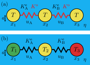
Figure 1: Two stochastic three-sphere micromachines consisting of three spheres with a radius $a$ and two springs with a natural length $\ell$. These micromachines are immersed in a fluid with viscosity $\eta$. The positions of the spheres are denoted by $x_{i}$ ($i=1,2,3$) in a one-dimensional coordinate, and the spring extensions with respect to $\ell$ are denoted by $u_{\alpha}$ ($\alpha={\rm A},{\rm B}$). (a) Odd three-sphere micromachine in which the two springs have the odd elastic constant $K^{\rm o}$ in addition to the even elastic constants $K^{\rm e}_{\rm A}$ and $K^{\rm e}_{\rm B}$. The temperature of all the spheres is $T$. The ratios are defined by $\kappa=K_{\rm B}^{\rm e}/K_{\rm A}^{\rm e}$ and $\lambda=K^{\rm o}/K_{\rm A}^{\rm e}$. (b) Thermal three-sphere micromachine in which the two springs have only the two elastic constants $K^{\rm e}_{\rm A}$ and $K^{\rm e}_{\rm B}$. However, the three spheres are in equilibrium with independent heat baths at different temperatures $T_{i}$ ($i=1,2,3$).

II.1 Model

We first describe the model of the odd micromachine that is slightly extended from our previous model Yasuda21 ; Kobayashi23 . As schematically shown in Fig. 1(a), this model consists of three spheres of radius $a$ positioned along a one-dimensional coordinate system, denoted by $x_{i}$ ($i=1,2,3$). These three spheres are connected by two springs that exhibit both even and odd elasticities. We denote the two spring extensions by $u_{\rm A}=x_{2}-x_{1}-\ell$ and $u_{\rm B}=x_{3}-x_{2}-\ell$, where $\ell$ is the constant natural length. Then the forces $F_{\rm A}$ and $F_{\rm B}$ conjugate to $u_{\rm A}$ and $u_{\rm B}$, respectively, are given by $F_{\alpha}=-K_{\alpha\beta}u_{\beta}$ ($\alpha,\beta={\rm A},{\rm B}$). For an odd elastic spring, the elastic constant matrix $K_{\alpha\beta}$ is given by

$$\mathbf{K}=\left(\begin{array}[]{cc}K_{\rm A}^{\rm e}&K^{\rm o}\vspace{1ex}\\ -K^{\rm o}&K_{\rm B}^{\rm e}\\ \end{array}\right).$$ (3)

In the two-dimensional configuration space, $K_{\rm A}^{\rm e}$ and $K_{\rm B}^{\rm e}$ are positive even elastic constants, while $K^{\rm o}$ is an odd elastic constant that can take both positive and negative values. In our previous study, we only studied the case of $K_{\rm A}^{\rm e}=K_{\rm B}^{\rm e}$ Yasuda21 ; Kobayashi23 . Then, the forces $f_{i}$ acting on each sphere are given by $f_{1}=-F_{\rm A}$, $f_{2}=F_{\rm A}-F_{\rm B}$, and $f_{3}=F_{\rm B}$. Notice that these forces automatically satisfy the force-free condition, i.e., $f_{1}+f_{2}+f_{3}=0$ Yasuda17a .

The above odd micromachine is immersed in a fluid of shear viscosity $\eta$ and temperature $T$. The Langevin equation of each sphere is given by DoiBook

$$\dot{x}_{i}=M_{ij}f_{j}+\xi_{i},$$ (4)

where $\dot{x}_{i}=dx_{i}/dt$ and $M_{ij}$ is hydrodynamic mobility coefficient matrix Najafi04 ; Golestanian08

$$M_{ij}=\begin{cases}1/(6\pi\eta a)&(i=j),\vspace{1ex}\\ 1/(4\pi\eta|x_{i}-x_{j}|)&(i\neq j).\end{cases}$$ (5)

In Eq. (4), the Gaussian white-noise sources $\xi_{i}$ have zero mean $\langle\xi_{i}(t)\rangle=0$, and their correlations satisfy the fluctuation-dissipation theorem DoiBook

$$\langle\xi_{i}(t)\xi_{j}(t^{\prime})\rangle=2k_{\rm B}TM_{ij}\delta(t-t^{\prime}),$$ (6)

where $k_{\rm B}$ is the Boltzmann constant. This condition assures that the surrounding fluid is in thermal equilibrium. Since the noise amplitudes depend on the particle positions, we use the Itô interpretation in Eq. (4) Kobayashi23 .

II.2 Average velocity

It is convenient to introduce the characteristic time scale $\tau=6\pi\eta a/K_{\rm A}^{\rm e}$ describing the spring relaxation time. We define the ratios between the elastic constants by $\kappa=K_{\rm B}^{\rm e}/K_{\rm A}^{\rm e}$ and $\lambda=K^{\rm o}/K_{\rm A}^{\rm e}$. In the following analysis, we assume $u_{\alpha}\ll\ell$ and $a\ll\ell$, and focus on the leading-order contribution. The instantaneous total velocity of the micromachine is simply given by $V=(\dot{x}_{1}+\dot{x}_{2}+\dot{x}_{3})/3$. Using Eqs. (3)-(5) and taking the statistical average, we obtain Yasuda21 ; Kobayashi23

$$\langle V\rangle =\frac{a}{8\ell^{2}\tau}\Big{[}(-1+3\lambda)\langle u_{\rm A}^{2}\rangle+(\kappa+3\lambda)\langle u_{\rm B}^{2}\rangle$$

$$+[3(1-\kappa)-2\lambda]\langle u_{\rm A}u_{\rm B}\rangle\Big{]},$$ (7)

where we have used $\langle u_{\alpha}\rangle=0$.

The equal-time correlation functions $\langle u_{\alpha}u_{\beta}\rangle$ appearing in Eq. (7) can be obtained from the reduced Langevin equations for $\dot{u}_{\rm A}=\dot{x}_{2}-\dot{x}_{1}$ and $\dot{u}_{\rm B}=\dot{x}_{3}-\dot{x}_{2}$ as

$$\dot{u}_{\alpha}=\Gamma_{\alpha\beta}u_{\beta}+\Xi_{\alpha},$$ (8)

where the friction matrix $\Gamma_{\alpha\beta}$ and the noise vector $\Xi_{\alpha}$ are given by

$$\mathbf{\Gamma}=-\frac{1}{\tau}\left(\begin{array}[]{cc}2+\lambda&-\kappa+2\lambda\\ -1-2\lambda&2\kappa-\lambda\\ \end{array}\right),\quad\mathbf{\Xi}=\left(\begin{array}[]{cc}\xi_{2}-\xi_{1}\\ \xi_{3}-\xi_{2}\\ \end{array}\right).$$ (13)

Here, under the assumption $u_{\alpha}\ll\ell$, we have neglected the hydrodynamic interactions acting between different spheres, i.e., $M_{ij}\approx 0$ when $i\neq j$ in Eq. (5). It should be noted that the friction matrix $\Gamma_{\alpha\beta}$ is nonreciprocal, i.e., $\Gamma_{\rm{AB}}\neq\Gamma_{\rm{BA}}$ when $\lambda\neq 0$ even if $\kappa=1$. Such a nonreciprocal interaction between $\langle u_{\rm A}\rangle$ and $\langle u_{\rm B}\rangle$ results from the odd elasticity $K^{\rm o}$.

To deal with the above Langevin equations, we introduce the bilateral Fourier transform of a function $f(t)$ as $f(\omega)=\int_{-\infty}^{\infty}dt\,f(t)e^{-{\rm i}\omega t}$ and its inverse transform as $f(t)=\int_{-\infty}^{\infty}(d\omega/2\pi)\,f(\omega)e^{{\rm i}\omega t}$. Solving Eq. (8) in the frequency domain, we obtain

$$u_{\rm A}(\omega) =\frac{\left[(2\kappa-\lambda)+{\rm i}\omega\tau\right]\xi_{1}(\omega)-\left[(\kappa+\lambda)+{\rm i}\omega\tau\right]\xi_{2}(\omega)-(\kappa-2\lambda)\xi_{3}(\omega)}{-3(\kappa+\lambda^{2})-2(1+\kappa){\rm i}\omega\tau+(\omega\tau)^{2}}\tau,$$ (14)

$$u_{\rm B}(\omega) =\frac{(1+2\lambda)\xi_{1}(\omega)+\left[(1-\lambda)+{\rm i}\omega\tau\right]\xi_{2}(\omega)-\left[(2+\lambda)+{\rm i}\omega\tau\right]\xi_{3}(\omega)}{-3(\kappa+\lambda^{2})-2(1+\kappa){\rm i}\omega\tau+(\omega\tau)^{2}}\tau.$$ (15)

Using Eqs. (14) and (15), one can calculate the correlation functions $\langle u_{\rm\alpha}(\omega)u_{\rm\beta}(\omega^{\prime})\rangle$. Then, the equal-time correlation functions are obtained as

$$\langle u_{\rm A}^{2}\rangle =\int_{-\infty}^{\infty}\frac{d\omega}{2\pi}\int_{-\infty}^{\infty}\frac{d\omega^{\prime}}{2\pi}\langle u_{\rm A}(\omega)u_{\rm A}(\omega^{\prime})\rangle$$

$$=\frac{k_{\rm B}T(\kappa+\kappa^{2}-\kappa\lambda+2\lambda^{2})}{K_{\rm A}^{\rm e}(1+\kappa)(\kappa+\lambda^{2})},$$ (16)

$$\langle u_{\rm B}^{2}\rangle =\frac{k_{\rm B}T(1+\kappa+\lambda+2\lambda^{2})}{K_{\rm A}^{\rm e}(1+\kappa)(\kappa+\lambda^{2})},$$ (17)

$$\langle u_{\rm A}u_{\rm B}\rangle =-\frac{k_{\rm B}T[(1-\kappa)\lambda+\lambda^{2}]}{K_{\rm A}^{\rm e}(1+\kappa)(\kappa+\lambda^{2})}.$$ (18)

Here, we have neglected the cross-correlations of the noise, $\langle\xi_{i}\xi_{j}\rangle$ with $i\neq j$, because they only contribute to the higher order terms in $a/\ell$. When $\lambda=0$, the above expressions reduce to $\langle u_{\rm A}^{2}\rangle=k_{\rm B}T/K_{\rm A}^{\rm e}$, $\langle u_{\rm B}^{2}\rangle=k_{\rm B}T/K_{\rm B}^{\rm e}$, and $\langle u_{\rm A}u_{\rm B}\rangle=0$, reproducing the well-known thermal equilibrium case.

Substituting the equal-time correlations in Eqs. (16)-(18) into Eq. (7), we obtain the steady state average velocity of the odd micromachine as

$$\langle V\rangle=\frac{7k_{\rm B}T\lambda}{24\pi\eta\ell^{2}(1+\kappa)},$$ (19)

which reduces to the previous result when $\kappa=1$ Yasuda21 ; Kobayashi23 . Recalling $\lambda=K^{\rm o}/K_{\rm A}^{\rm e}$, we see that $\langle V\rangle$ is proportional to the odd elastic constant $K^{\rm o}$ whose sign determines the swimming direction. Since $\langle V\rangle$ is also proportional to $k_{\rm B}T$, thermal fluctuations are responsible for the locomotion of the odd micromachine.

II.3 Entropy production rate

Next, we calculate the steady state average entropy production rate $\langle\dot{\sigma}\rangle$ of the odd three-sphere micromachine, which is given by

$$\langle\dot{\sigma}\rangle=-\sum_{i=1}^{3}\frac{\langle\dot{Q}_{i}\rangle}{T}.$$ (20)

According to the framework of stochastic energetics established by Sekimoto SekimotoBook , the time-derivative of the heat gained by the $i$-th sphere is

$$\dot{Q}_{i}=6\pi\eta a(-\dot{x}_{i}+\xi_{i})\circ\dot{x}_{i},$$ (21)

where $\dot{x}_{i}$ and $\xi_{i}$ are given by Eq. (4) and $\circ$ indicates the Stratonovich product (the summation over $i$ is not taken in this expression). Then, the lowest-order average heat flows become

$${\langle\dot{Q}_{1}\rangle} =\frac{k_{\rm B}T\lambda(1-2\lambda)}{\tau(1+\kappa)},$$ (22)

$${\langle\dot{Q}_{2}\rangle} =\frac{k_{\rm B}T\lambda(-1+\kappa-2\lambda)}{\tau(1+\kappa)},$$ (23)

$${\langle\dot{Q}_{3}\rangle} =-\frac{k_{\rm B}T\lambda(\kappa+2\lambda)}{\tau(1+\kappa)},$$ (24)

which all vanish when $\lambda=0$. Substituting Eqs. (22)-(24) into Eq. (20), we obtain the average entropy production rate of the odd micromachine as

$$\langle\dot{\sigma}\rangle=\frac{6k_{\rm B}\lambda^{2}}{\tau(1+\kappa)},$$ (25)

which is obviously non-negative, $\langle\dot{\sigma}\rangle\geq 0$, and vanishes only when $\lambda=0$. This result is consistent with the second law for nonequilibrium steady states Freitas22 .

In our previous work with $\kappa=1$ Yasuda21 , we obtained the entropy production rate by using the combination of the friction matrix and the covariant matrix of the Gaussian distribution function Weiss03 ; Weiss07 . We also showed that the entropy production rate coincides with the power (work per unit time) of the odd micromachine. Hence, all the extracted work due to odd elasticity is converted into entropy production in the steady state.

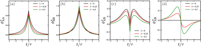
Figure 2: Plots of the scaled extension-extension correlation functions (a) $\phi_{\rm{AA}}^{\rm s}$, (b) $\phi_{\rm{BB}}^{\rm s}$, (c) $\phi_{\rm{AB}}^{\rm s}$, and (d) $\phi_{\rm{AB}}^{\rm a}$ as a function of $t/\tau$ for $\kappa=1$. The dimensionless odd elasticity is chosen as $\lambda=0$ (black), $0.25$ (red), and $5$ (green). For these parameters, $\mu=\sqrt{3\lambda^{2}-(1-\kappa+\kappa^{2})}$ is purely imaginary, and the correlation functions do not exhibit any oscillatory behaviors.

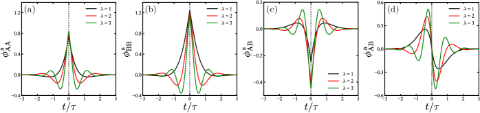
Figure 3: Plots of the scaled extension-extension correlation functions (a) $\phi_{\rm{AA}}^{\rm s}$, (b) $\phi_{\rm{BB}}^{\rm s}$, (c) $\phi_{\rm{AB}}^{\rm s}$, and (d) $\phi_{\rm{AB}}^{\rm a}$ as a function of $t/\tau$ for $\kappa=1$. The dimensionless odd elasticity is chosen as $\lambda=1$ (black), $2$ (red), and $3$ (green). For these parameters, $\mu=\sqrt{3\lambda^{2}-(1-\kappa+\kappa^{2})}$ is real and the correlation functions exhibit oscillatory behaviors.

II.4 Time-correlation functions

Next, we calculate the time-correlation functions of the odd micromachine in the steady state. Using Eqs. (14) and (15), we perform inverse Fourier transform and obtain the extension-extension time-correlation function matrix $\phi_{\alpha\beta}(t)$ defined by

$$\langle u_{\alpha}(t)u_{\beta}(0)\rangle=\frac{k_{\rm B}T}{K_{\rm A}^{\rm e}}\phi_{\alpha\beta}(t),$$ (26)

where $\phi_{\alpha\beta}$ is dimensionless. Generally, one can decompose the time-correlation functions into the symmetric and antisymmetric parts as YasudaTCF22 ; KobayashiODD23

$$\phi_{\alpha\beta}(t)=\phi_{\alpha\beta}^{\mathrm{s}}(t)+\phi_{\alpha\beta}^{\mathrm{a}}(t),$$ (27)

where $\phi_{\alpha\beta}^{\mathrm{s}}(t)=\phi_{\beta\alpha}^{\mathrm{s}}(t)$ and $\phi_{\alpha\beta}^{\mathrm{a}}(t)=-\phi_{\beta\alpha}^{\mathrm{a}}(t)$. When $\alpha=\beta$ (auto-correlation), only the symmetric part is allowed due to the time-translational invariance of the steady state and hence the antisymmetric parts should vanish, i.e., $\phi_{\rm{AA}}^{\rm a}=\phi_{\rm{BB}}^{\rm a}=0$. When $\alpha\neq\beta$ (cross-correlation) and if the system is in thermal equilibrium, the antisymmetric part of the cross-correlation $\phi_{\rm{AB}}^{\rm a}$ should also vanish due to the time-reversal symmetry DoiBook . In nonequilibrium situations, however, $\phi_{\rm{AB}}^{\rm a}$ can exist because the time-reversal symmetry is generally broken YasudaTCF22 ; KobayashiODD23 . In other words, $\phi_{\rm{AB}}^{\rm a}$ quantifies the degree of nonequilibrium in stochastic micromachines.

The inverse Fourier transform of the correlation function can be straightforwardly performed by employing the residue theorem. After some calculation, we obtain the time-dependent extension-extension correlation functions as

$$\phi_{\rm{AA}}^{\rm s}(t) =\frac{\kappa+\kappa^{2}-\kappa\lambda+2\lambda^{2}}{(1+\kappa)(\kappa+\lambda^{2})}\cos\left(\mu t/\tau\right)e^{-(1+\kappa)|t|/\tau}$$

$$-\frac{\kappa(1-\kappa+\lambda)}{(\kappa+\lambda^{2})\mu}\sin\left(\mu|t|/\tau\right)e^{-(1+\kappa)|t|/\tau},$$ (28)

$$\phi_{\rm{BB}}^{\rm s}(t) =\frac{1+\kappa+\lambda+2\lambda^{2}}{(1+\kappa)(\kappa+\lambda^{2})}\cos\left(\mu t/\tau\right)e^{-(1+\kappa)|t|/\tau}$$

$$+\frac{1-\kappa+\lambda}{(\kappa+\lambda^{2})\mu}\sin\left(\mu|t|/\tau\right)e^{-(1+\kappa)|t|/\tau},$$ (29)

$$\phi_{\rm{AB}}^{\rm s}(t) =-\frac{(1-\kappa)\lambda+\lambda^{2}}{(1+\kappa)(\kappa+\lambda^{2})}\cos\left(\mu t/\tau\right)e^{-(1+\kappa)|t|/\tau}$$

$$+\frac{\kappa-(1-\kappa)\lambda}{(\kappa+\lambda^{2})\mu}\sin\left(\mu|t|/\tau\right)e^{-(1+\kappa)|t|/\tau},$$ (30)

$$\phi_{\rm{AB}}^{\rm a}(t) =-\frac{3\lambda}{(1+\kappa)\mu}\sin\left(\mu t/\tau\right)e^{-(1+\kappa)|t|/\tau},$$ (31)

where we have used the notation $\mu=\sqrt{3\lambda^{2}-(1-\kappa+\kappa^{2})}$. When $\lambda^{2}<(1-\kappa+\kappa^{2})/3$, $\mu$ is purely imaginary so that “$\cos$” and “$\sin$” functions should be regarded as “$\cosh$” and “$\sinh$” functions, respectively. The equal-time correlations in Eqs. (16)-(18) can be recovered by setting $t=0$ in the above equations.

As mentioned before, the auto-correlations have only the symmetric parts $\phi_{\rm{AA}}^{\rm s}$ and $\phi_{\rm{BB}}^{\rm s}$, whereas the cross-correlation contains both the symmetric part $\phi_{\rm{AB}}^{\rm s}$ and the antisymmetric part $\phi_{\rm{AB}}^{\rm a}$. However, $\phi_{\rm{AB}}^{\rm a}$ exists only for nonzero $\lambda$ and measures the degree of the broken time-reversal symmetry. Obviously, the symmetric parts are even functions in time, and the antisymmetric part is an odd function in time. In Fig. 2, we plot (a) $\phi_{\rm{AA}}^{\rm s}$, (b) $\phi_{\rm{BB}}^{\rm s}$, (c) $\phi_{\rm{AB}}^{\rm s}$, and (d) $\phi_{\rm{AB}}^{\rm a}$ as a function of $t/\tau$ when $\kappa=1$ and $\lambda=0,0.25,0.5$ (when $\mu$ is imaginary). In Fig. 3, we plot the same functions when $\kappa=1$ and $\lambda=1,2,3$ (when $\mu$ is real). In Figs. 2(a) and (b), the auto-correlation functions decay monotonically, whereas the symmetric part of the cross-correlation function exhibits maximum values and even takes negative values in Figs. 2(c). As we increase the odd elasticity $\lambda$ in Fig. 3, the oscillatory behaviors of the time-correlation functions become pronounced.

The velocity-velocity correlation function matrix $\psi_{\alpha\beta}(t)$ can be obtained by taking the second time derivative of the extension-extension correlation functions as DoiBook

$$\langle\dot{u}_{\alpha}(t)\dot{u}_{\beta}(0)\rangle=-\frac{\partial^{2}}{\partial t^{2}}\langle u_{\alpha}(t)u_{\beta}(0)\rangle=\frac{D}{\tau}\psi_{\alpha\beta}(t),$$ (32)

where we have introduced the diffusion coefficient of a sphere $D=k_{\rm B}T/(6\pi\eta a)$. Alternatively, one can also use Eq. (8) to calculate $\langle\dot{u}_{\alpha}(t)\dot{u}_{\beta}(0)\rangle$ directly, as shown in Appendix A. Similar to Eq. (27), $\psi_{\alpha\beta}(t)$ can be decomposed into the symmetric and antisymmetric parts as $\psi_{\alpha\beta}(t)=\psi_{\alpha\beta}^{\mathrm{s}}(t)+\psi_{\alpha\beta}^{\mathrm{a}}(t)$. Following the same argument as before, we have $\psi_{\rm{AA}}^{\rm a}=\psi_{\rm{BB}}^{\rm a}=0$ for the auto-correlation functions. However, the antisymmetric part of the cross-correlation $\psi_{\rm{AB}}^{\rm a}$ exists when $\lambda$ is nonzero.

The explicit expressions of the velocity-velocity correlation functions and their plots are given in Appendix A. We note that the symmetric part of the velocity-velocity correlation functions has a sharp peak at $t=0$, which arises from the noise term in the Langevin equation. For very short time, $t\ll\tau$, the velocity-velocity correlation functions are approximated as DoiBook

$$\langle\dot{u}_{\rm A}(t)\dot{u}_{\rm A}(0)\rangle =\langle\dot{u}_{\rm B}(t)\dot{u}_{\rm B}(0)\rangle\approx 4D\delta(t),$$ (33)

$$\langle\dot{u}_{\rm A}(t)\dot{u}_{\rm B}(0)\rangle =\langle\dot{u}_{\rm B}(t)\dot{u}_{\rm A}(0)\rangle\approx-2D\delta(t).$$ (34)

II.5 Green-Kubo relations

At equilibrium, the time integral of the velocity-velocity correlation function for a free particle gives the diffusion coefficient, known as one of the Green-Kubo relations Zwanzig . Recently, Han et al. argued that an equilibrium-like Green-Kubo relation holds near the steady state of an isotropic active fluid if the activated and fluctuating degrees of freedom are statistically decoupled Han21 . Epstein and Mandadapu obtained the Green-Kubo relation for the odd viscosity Avron98 , which explicitly violates the time-reversal symmetry at the level of the steady state stress fluctuations Epstein20 ; Hargus20 .

For the odd micromachine, we perform the time integral of the velocity-velocity correlation functions given in Appendix A. From the auto-correlation functions in Eqs. (62) and (63), we obtain

$$\int_{0}^{\infty}dt\,\langle\dot{u}_{\rm A}(t)\dot{u}_{\rm A}(0)\rangle=\int_{0}^{\infty}dt\,\langle\dot{u}_{\rm B}(t)\dot{u}_{\rm B}(0)\rangle=0.$$ (35)

Here, the time integral of Eq. (33) gives $2D$ which is canceled by the rest of the terms in Eqs. (62) and (63). The result that the integrals in Eq. (35) vanish is reasonable because the particles are connected by the springs DoiBook .

For the cross-correlation functions in Eqs. (64)-(65), on the other hand, one obtains

$$\int_{0}^{\infty}dt\,\left[\langle\dot{u}_{\rm A}(t)\dot{u}_{\rm B}(0)\rangle-\langle\dot{u}_{\rm B}(t)\dot{u}_{\rm A}(0)\rangle\right]=-\frac{6\lambda D}{1+\kappa}.$$ (36)

In this calculation, only the antisymmetric part of the correlation function $\psi_{\rm AB}^{\mathrm{a}}$ remains. Equation (36) explicitly demonstrates that the broken time-reversal symmetry is caused by the finite odd elasticity $\lambda$. The above result also suggests that one can estimate the odd elasticity of a micromachine by measuring the cross-correlation function KobayashiODD23 .

III Thermal three-sphere micromachine

III.1 Model

In this section, we discuss another type of stochastic micromachine that is also purely driven by thermal fluctuation but without any explicit odd elasticity. Here, the key assumption is that the three spheres are in equilibrium with independent heat baths having different temperatures Hosaka17 ; Sou19 ; Sou21 . In this micromachine, the heat transfer occurs from a hotter sphere to a colder one, driving the whole system out of equilibrium.

As shown in Fig. 1(b), we consider a three-sphere micromachine in which the three spheres are in equilibrium with independent heat baths having different temperatures $T_{i}$ ($i=1,2,3$) Hosaka17 ; Sou19 ; Sou21 . On the other hand, the two springs have only even elasticity characterized by $K_{\rm A}^{\rm e}$ and $K_{\rm B}^{\rm e}$, whereas an explicit odd elastic constant does not exist. The equation of motion of each sphere is the same as in Eq. (4), although the thermal noise $\xi_{i}$ has different statistical properties. For the thermal micromachine, we assume that Gaussian white-noise sources $\xi_{i}$ have zero mean $\langle\xi_{i}(t)\rangle_{\rm t}=0$, and their correlations satisfy

$$\langle\xi_{i}(t)\xi_{j}(t^{\prime})\rangle_{\rm t}=2D_{ij}\delta(t-t^{\prime}).$$ (37)

Here, $D_{ij}$ is the mutual diffusion coefficient matrix given by

$$D_{ij}=\begin{cases}k_{\rm B}T_{i}/(6\pi\eta a)&(i=j),\vspace{1ex}\\ k_{\rm B}\Theta(T_{i},T_{j})/(4\pi\eta|x_{i}-x_{j}|)&(i\neq j),\end{cases}$$ (38)

where $\Theta(T_{i},T_{j})$ is a function of $T_{i}$ and $T_{j}$. The effective temperature $\Theta$ can be the mobility-weighted average Grosberg15 , which in the present case is simply given by $\Theta(T_{i},T_{j})=(T_{i}+T_{j})/2$ because all the spheres have the same size. However, its explicit functional form is not needed here, and we only require that $\Theta$ should satisfy an appropriate fluctuation-dissipation theorem in thermal equilibrium. Such a simplification is justified because we only consider the limit of $a\ll\ell$.

III.2 Average velocity

The average velocity of the thermal micromachine can be obtained similarly as before by using Eq. (7) with $\lambda=0$ because odd elasticity does not exist in this model. In our previous paper, the average velocity was obtained as Hosaka17

$$\langle V\rangle_{\rm t}=\frac{k_{\rm B}T_{2}\left[(2-5\kappa)\theta_{1}-7(1-\kappa)+(5-2\kappa)\theta_{3}\right]}{144\pi\eta\ell^{2}(1+\kappa)},$$ (39)

where $\kappa=K_{\rm B}^{\rm e}/K_{\rm A}^{\rm e}$ as before and we have defined the temperature ratios by $\theta_{1}=T_{1}/T_{2}$ and $\theta_{3}=T_{3}/T_{2}$. When the three temperatures are identical, $T_{1}=T_{2}=T_{3}$ or $\theta_{1}=\theta_{3}=1$, the velocity vanishes identically, $\langle V\rangle_{\rm t}=0$. This means that the temperature difference among the spheres causes the locomotion of the thermal three-sphere micromachine.

When the two springs are equivalent and $\kappa=1$, $\langle V\rangle_{\rm t}$ does not depend on $T_{2}$ and is proportional to the temperature difference $T_{3}-T_{1}$. In this case, the average velocity vanishes when $T_{1}=T_{3}$ even though $T_{1}$ and $T_{3}$ are different from $T_{2}$.

III.3 Entropy production rate

The average entropy production rate can also be calculated similarly to the previous section. For the thermal micromachine, the lowest-order average heat flows were obtained as Hosaka17

$$\langle\dot{Q}_{1}\rangle_{\rm t} =\frac{k_{\rm B}T_{2}[(3+2\kappa)\theta_{1}-(3+\kappa)-\kappa\theta_{3}]}{6\tau(1+\kappa)},$$ (40)

$$\langle\dot{Q}_{2}\rangle_{\rm t} =\frac{k_{\rm B}T_{2}[-(3+\kappa)\theta_{1}+(3+2\kappa+3\kappa^{2})-(\kappa+3\kappa^{2})\theta_{3}]}{6\tau(1+\kappa)},$$ (41)

$$\langle\dot{Q}_{3}\rangle_{\rm t} =\frac{k_{\rm B}T_{2}[-\kappa\theta_{1}-(\kappa+3\kappa^{2})+(2\kappa+3\kappa^{2})\theta_{3}]}{6\tau(1+\kappa)},$$ (42)

which all vanish when $T_{1}=T_{2}=T_{3}$ or $\theta_{1}=\theta_{3}=1$. It is worth to note that the above heat flows satisfy $\langle\dot{Q}_{1}\rangle_{\rm t}+\langle\dot{Q}_{2}\rangle_{\rm t}+\langle\dot{Q}_{3}\rangle_{\rm t}=0$ so that the total heat is conserved.

Using these results and keeping in mind the different temperatures of the spheres, the steady state average entropy production rate is given by

$$\langle\dot{\sigma}\rangle_{\rm t}= -\sum_{i=1}^{3}\frac{\langle\dot{Q}_{i}\rangle_{\rm t}}{T_{i}}$$

$$= \frac{k_{\rm B}}{6\tau(1+\kappa)}\Biggl{[}(3+\kappa)\left(\theta_{1}+\frac{1}{\theta_{1}}\right)+\kappa\left(\frac{\theta_{1}}{\theta_{3}}+\frac{\theta_{3}}{\theta_{1}}\right)$$

$$+\kappa(1+3\kappa)\left(\theta_{3}+\frac{1}{\theta_{3}}\right)-6(1+\kappa+\kappa^{2})\Biggr{]}.$$ (43)

One can easily confirm the second law, $\langle\dot{\sigma}\rangle_{\rm t}\geq 0$, by using the inequality $A+B\geq 2\sqrt{AB}$ for $A,B>0$ and $\langle\dot{\sigma}\rangle_{\rm t}$ vanishes when $\theta_{1}=\theta_{3}=1$. The above entropy production rate reduces to that in Ref. Sou21 when $\kappa=1$.

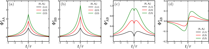
Figure 4: Plots of the scaled extension-extension correlation functions (a) $\Phi_{\rm{AA}}^{\rm s}$, (b) $\Phi_{\rm{BB}}^{\rm s}$, (c) $\Phi_{\rm{AB}}^{\rm s}$, and (d) $\Phi_{\rm{AB}}^{\rm a}$ as a function of $t/\tau$ for $\kappa=1$. The dimensionless temperature ratios between the spheres are chosen as $(\theta_{1},\theta_{3})=(1,1)$ (black), $(2,3)$ (red), and $(3,5)$ (green).

III.4 Time-correlation functions

Next, we calculate the extension-extension time-correlation function matrix $\Phi_{\alpha\beta}$ for the thermal micromachine and decompose it into the symmetric and antisymmetric parts as

$$\langle u_{\alpha}(t)u_{\beta}(0)\rangle_{\rm t}=\frac{k_{\rm B}T_{2}}{K_{\rm A}^{\rm e}}\Phi_{\alpha\beta}(t)=\frac{k_{\rm B}T_{2}}{K_{\rm A}^{\rm e}}\left[\Phi_{\alpha\beta}^{\mathrm{s}}(t)+\Phi_{\alpha\beta}^{\mathrm{a}}(t)\right].$$ (44)

The time-translational invariance requiers $\Phi_{\rm{AA}}^{\rm a}=\Phi_{\rm{BB}}^{\rm a}=0$ as before. After repeating similar calculations, we obtain

$$\Phi_{\rm AA}^{\mathrm{s}}(t) =\frac{(3+4\kappa)\theta_{1}+(3+\kappa)+\kappa\theta_{3}}{6(1+\kappa)}\cosh\left(\rho t/\tau\right)e^{-(1+\kappa)|t|/\tau}$$

$$+\frac{(-3+4\kappa)\theta_{1}-(3-\kappa)+\kappa\theta_{3}}{6\rho}\sinh\left(\rho|t|/\tau\right)e^{-(1+\kappa)|t|/\tau},$$ (45)

$$\Phi_{\rm BB}^{\mathrm{s}}(t) =\frac{\theta_{1}+(1+3\kappa)+(4+3\kappa)\theta_{3}}{6\kappa(1+\kappa)}\cosh\left(\rho t/\tau\right)e^{-(1+\kappa)|t|/\tau}$$

$$+\frac{\theta_{1}+(1-3\kappa)+(4-3\kappa)\theta_{3}}{6\kappa\rho}\sinh\left(\rho|t|/\tau\right)e^{-(1+\kappa)|t|/\tau},$$ (46)

$$\Phi_{\rm{AB}}^{\rm s}(t) =\frac{\theta_{1}-2+\theta_{3}}{3(1+\kappa)}\cosh\left(\rho t/\tau\right)e^{-(1+\kappa)|t|/\tau}$$

$$+\frac{\theta_{1}+1+\theta_{3}}{3\rho}\sinh\left(\rho|t|/\tau\right)e^{-(1+\kappa)|t|/\tau},$$ (47)

$$\Phi_{\rm{AB}}^{\rm a}(t) =\frac{-\theta_{1}+(1-\kappa)+\kappa\theta_{3}}{2(1+\kappa)\rho}\sinh\left(\rho t/\tau\right)e^{-(1+\kappa)|t|/\tau},$$ (48)

where we have used the notation $\rho=\sqrt{1-\kappa+\kappa^{2}}$. Since $1-\kappa+\kappa^{2}>0$, $\rho$ is real for any $\kappa$, and all the above time-correlation functions do not oscillate in time. In Eq. (48), we see that $\Phi_{\rm{AB}}^{\rm a}(t)$ vanishes when $\theta_{1}=\theta_{3}=1$.

Next, we calculate the velocity-velocity correlation function matrix $\Psi_{\alpha\beta}(t)$ for the thermal micromachine as

$$\langle\dot{u}_{\alpha}(t)\dot{u}_{\beta}(0)\rangle_{\rm t}=\frac{D_{22}}{\tau}\Psi_{\alpha\beta}(t)=\frac{D_{22}}{\tau}\left[\Psi_{\alpha\beta}^{\mathrm{s}}(t)+\Psi_{\alpha\beta}^{\mathrm{a}}(t)\right],$$ (49)

where $D_{22}=k_{\rm B}T_{2}/(6\pi\eta a)$ is the diffusion coefficient defined by using the temperature $T_{2}$ [see Eq. (38)]. The explicit expressions of the velocity-velocity correlation functions and their plots are given in Appendix B. Similar to the odd micromachine, the symmetric parts of the velocity-velocity correlation functions have a sharp peak at $t=0$. In the short time limit, $t\ll\tau$, the velocity-velocity correlation functions become

$$\langle\dot{u}_{\rm A}(t)\dot{u}_{\rm A}(0)\rangle_{\rm t} \approx 2(\theta_{1}+1)D_{22}\delta(t),$$ (50)

$$\langle\dot{u}_{\rm B}(t)\dot{u}_{\rm B}(0)\rangle_{\rm t} \approx 2(1+\theta_{3})D_{22}\delta(t),$$ (51)

$$\langle\dot{u}_{\rm A}(t)\dot{u}_{\rm B}(0)\rangle_{\rm t} =\langle\dot{u}_{\rm B}(t)\dot{u}_{\rm A}(0)\rangle_{\rm t}\approx-2D_{22}\delta(t).$$ (52)

These results coincide with Eqs. (33) and (34) when $\theta_{1}=\theta_{3}=1$ and if $D_{22}$ can be identified with $D$.

III.5 Green-Kubo relations

Having obtained the velocity-velocity correlation functions for the thermal micromachine, we now calculate the Green-Kubo relations as in the previous section. From the auto-correlation functions in Eqs. (66) and (67), we have

$$\int_{0}^{\infty}dt\,\langle\dot{u}_{\rm A}(t)\dot{u}_{\rm A}(0)\rangle_{\rm t}=\int_{0}^{\infty}dt\,\langle\dot{u}_{\rm B}(t)\dot{u}_{\rm B}(0)\rangle_{\rm t}=0,$$ (53)

similar to Eq. (35). From the cross-correlation functions in Eqs. (68) and (69), however, we obtain

$$\int_{0}^{\infty}dt\,\left[\langle\dot{u}_{\rm A}(t)\dot{u}_{\rm B}(0)\rangle_{\rm t}-\langle\dot{u}_{\rm B}(t)\dot{u}_{\rm A}(0)\rangle_{\rm t}\right]$$

$$=-\frac{[\theta_{1}-(1-\kappa)-\kappa\theta_{3}]D_{22}}{1+\kappa}.$$ (54)

This result implies that the time-reversal symmetry is broken for the thermal microswimmer when the temperatures are different.

IV Effective odd elasticity of the thermal micromachine

So far, we have discussed the statistical properties of the odd and thermal micromachines, and obtained their time-correlation functions to discuss the Green-Kubo relations. Although these two stochastic models are different, it is worthwhile to consider the effective odd elasticity of the thermal micromachine. As we mentioned earlier, odd elasticity gives a quantitative measure of the work that can be extracted from active systems Scheibner20 ; Fruchart23 , and nonequilibrium cyclic dynamics of micromachines can be quantified by effective odd elasticity Yasuda21catalytic ; YasudaOM22 . Such an approach is possible for stochastic micromachines by looking at the violation of the time-reversal symmetry of the cross-correlation functions YasudaTCF22 ; KobayashiODD23 .

For this purpose, we compare the Green-Kubo relations in Eqs. (36) and (54), and define an effective odd elasticity $\lambda_{\rm t}$ ratio of the thermal micromachine as

$$\lambda_{\rm t}=\frac{D_{22}}{6D}[\theta_{1}-(1-\kappa)-\kappa\theta_{3}].$$ (55)

If we further assume $D_{22}=D$ and $\kappa=1$, we obtain

$$\lambda_{\rm t}=\frac{T_{1}-T_{3}}{6T_{2}}.$$ (56)

This result clearly demonstrates that the effective odd elasticity of the thermal micromachine is purely determined by the temperature difference between the edge spheres. The above relations further indicate that $\lambda_{\rm t}$ is inversely proportional to the middle sphere temperature $T_{2}$.

It should be mentioned, however, that the above argument is not the only way to obtain the effective odd elasticity of the thermal micromachine. For example, one can also compare the average velocities of the two micromachines as given in Eqs. (19) and (39) or the entropy production rates in Eqs. (25) and (43). Although the comparison of different quantities leads to a slightly modified numerical factor, the effective odd elasticity is always proportional to the temperature difference among the spheres, as shown in Eq. (56). This is because both the odd elasticity and the temperature difference lead to the violation of the time-reversal symmetry. One of the advantages of using the Green-Kubo relations to define $\lambda_{\rm t}$ is that they contain information on the cross-correlation functions over the whole time.

V Summary and discussion

In this paper, we have calculated the time-correlation functions of the two different stochastic three-sphere micromachines, i,e., the odd micromachine and the thermal micromachine. For both models, the cross-correlation functions of the two springs contain the antisymmetric part, which is a direct consequence of the broken time-reversal symmetry of the micromachines. For the odd micromachine, the antisymmetric part of the correlation function is proportional to the odd elastic constant [see Eq. (31)], whereas it is proportional to the temperature difference among the spheres [see Eq. (48)]. We have also obtained the entropy production rate and the Green-Kubo relations for the two micromachines. A comparison of these results allows us to discuss the effective odd elasticity of the thermal micromachine [see Eq. (55)], even though the odd elasticity is not explicitly included in the model. For the thermal micromachine, the effective odd elasticity is proportional to the temperature difference between the spheres, which causes an internal heat flow and leads to directional locomotion.

Evaluation of effective odd elasticity was previously discussed for a model micromachine driven by catalytic chemical reactions KobayashiODD23 . We calculated the time-correlation functions of the structural variables and analyzed them in terms of Langevin dynamics with effective odd elasticity YasudaTCF22 . It was also shown that the odd elasticity is directly related to the quantity called nonreciprocality of a micromachine. For a deterministic micromachine undergoing cyclic motions, the nonreciprocality $R$ is defined by Yasuda21

$$R=\frac{1}{2}\oint dt\,(u_{\rm A}\dot{u}_{\rm B}-\dot{u}_{\rm A}u_{\rm B}),$$ (57)

where the integral is taken over one cycle, and $R$ represents the area enclosed by the trajectory in the configuration space Shapere89 . For stochastic micromachines, the average nonreciprocality $\langle R\rangle$ is essentially given by the time derivative of the antisymmetric part of the extension-extension correlation function, such as given by Eq. (31) that is proportional to the odd elasticity. Hence, the effective odd elasticity introduced in Eq. (56) directly characterizes the nonreciprocality of the thermal micromachines.

Recently, Hargus et al. discussed odd diffusivity in two-dimensional chiral active matter and derived the Green-Kubo relation for the odd diffusion coefficient Hargus20prl . A similar relation was also obtained for the odd mobility of a passive tracer in a chiral active fluid Poggioli23 . In their results, both odd diffusivity and odd mobility result from the broken time-reversal symmetry in active systems and are related to the antisymmetric part of the cross-correlation functions, which is similar to our result. In our stochastic micromachines, the integrals of the auto-correlations vanish as in Eqs. (35) and (53) because the spheres are connected by the springs. Although the motions of the micromachines are one-dimensional in our models, the configurational space spanned by $u_{\rm A}$ and $u_{\rm B}$ are two-dimensional. It is useful to consider an effective odd elasticity in such a configurational space, and the obtained Green-Kubo relations for the cross-correlation functions in Eqs. (36) and (54) are directly proportional to the odd elasticity. We also note that the oscillatory trajectory seen in the chiral random walk Hargus20prl is analogous to the oscillatory behaviors of the time-correlation functions in this paper due to the odd elasticity.

In this work, the elastic constant matrix for the odd micromachine was given by Eq. (3) in which we took into account the difference between $K_{\rm A}^{\rm e}$ and $K_{\rm B}^{\rm e}$. However, the most general form of the elastic constant matrix can take the form

$$\mathbf{K}=\left(\begin{array}[]{cc}K_{\rm A}^{\rm e}&K^{\rm e}_{\rm AB}+K^{\rm o}\vspace{1ex}\\ K^{\rm e}_{\rm AB}-K^{\rm o}&K_{\rm B}^{\rm e}\\ \end{array}\right),$$ (60)

where we have introduced another even elastic constant $K^{\rm e}_{\rm AB}$ in the off-diagonal components KobayashiODD23 . Such an even elasticity can induce amplitude asymmetry between the two springs Lin23 . Although the time-correlation functions can be easily calculated in the presence of $K^{\rm e}_{\rm AB}$, Eq. (3) is sufficient to compare with the thermal micromachine.

To calculate the time-correlation functions, we have neglected hydrodynamic interactions acting between the spheres. This is justified because hydrodynamic interactions are higher-order contributions for the correlation functions, which will be calculated in our future work. It should be mentioned again, however, that hydrodynamic interactions are necessary for the locomotion of the three-sphere micromachines.

Appendix A Velocity-velocity correlation functions of the odd three-sphere micromachine

As mentioned in the text, the velocity-velocity correlation functions can be calculated by using Eq. (8) as

$$\langle\dot{u}_{\alpha}(t)\dot{u}_{\beta}(0)\rangle =\langle[\Gamma_{\alpha\gamma}u_{\gamma}(t)+\Xi_{\alpha}(t)][\Gamma_{\beta\delta}u_{\delta}(0)+\Xi_{\beta}(0)]\rangle.$$ (61)

The correlations between the displacement and noise, $\langle u_{\alpha}(t)\Xi_{\beta}(0)\rangle$, can also be calculated straightforwardly.

For the odd micromachine, the expressions of the velocity-velocity correlation functions defined in Eq. (32) are given as follows:

$$\psi_{\rm{AA}}^{\rm s}(t) =4\tau\delta(t)+\frac{6\lambda^{2}-3\kappa\lambda-(4+5\kappa+\kappa^{2})}{1+\kappa}\cos\left(\mu t/\tau\right)e^{-(1+\kappa)|t|/\tau}-\frac{12\lambda^{2}-3\kappa\lambda-(4-\kappa+\kappa^{2})}{\mu}\sin\left(\mu|t|/\tau\right)e^{-(1+\kappa)|t|/\tau},$$ (62)

$$\psi_{\rm{BB}}^{\rm s}(t) =4\tau\delta(t)+\frac{6\lambda^{2}+3\lambda-(1+5\kappa+4\kappa^{2})}{1+\kappa}\cos\left(\mu t/\tau\right)e^{-(1+\kappa)|t|/\tau}-\frac{12\lambda^{2}+3\lambda-(1-\kappa+4\kappa^{2})}{\mu}\sin\left(\mu|t|/\tau\right)e^{-(1+\kappa)|t|/\tau},$$ (63)

$$\psi_{\rm{AB}}^{\rm s}(t) =-2\tau\delta(t)$$

$$-\frac{3\lambda^{2}+3(1-\kappa)\lambda-2(1+2\kappa+\kappa^{2})}{1+\kappa}\cos\left(\mu t/\tau\right)e^{-(1+\kappa)|t|/\tau}+\frac{6\lambda^{2}+3(1-\kappa)\lambda-(2+\kappa+2\kappa^{2})}{\mu}\sin\left(\mu|t|/\tau\right)e^{-(1+\kappa)|t|/\tau},$$ (64)

$$\psi_{\rm{AB}}^{\rm a}(t) =\begin{cases}-6\lambda\cos\left(\mu t/\tau\right)e^{-(1+\kappa)t/\tau}-\dfrac{3\lambda[3\lambda^{2}-(2+\kappa+2\kappa^{2})]}{(1+\kappa)\mu}\sin\left(\mu t/\tau\right)e^{-(1+\kappa)t/\tau}&(t>0),\vspace{1ex}\\ 6\lambda\cos\left(\mu t/\tau\right)e^{(1+\kappa)t/\tau}-\dfrac{3\lambda[3\lambda^{2}-(2+\kappa+2\kappa^{2})]}{(1+\kappa)\mu}\sin\left(\mu t/\tau\right)e^{(1+\kappa)t/\tau}&(t<0),\end{cases}$$ (65)

where $\mu=\sqrt{3\lambda^{2}-(1-\kappa+\kappa^{2})}$.

Appendix B Velocity-velocity correlation functions of the thermal three-sphere micromachine

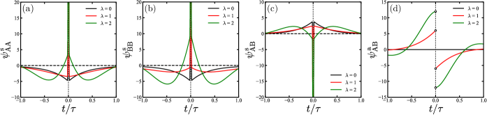
Figure 5: Plots of the scaled velocity-velocity correlation functions (a) $\psi_{\rm{AA}}^{\rm s}$, (b) $\psi_{\rm{BB}}^{\rm s}$, (c) $\psi_{\rm{AB}}^{\rm s}$, and (d) $\psi_{\rm{AB}}^{\rm a}$ as a function of $t/\tau$ for $\kappa=1$. The dimensionless odd elasticity is chosen as $\lambda=0$ (black), $1$ (red), and $2$ (green).

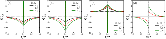
Figure 6: Plots of the scaled velocity-velocity correlation functions (a) $\Psi_{\rm{AA}}^{\rm s}$, (b) $\Psi_{\rm{BB}}^{\rm s}$, (c) $\Psi_{\rm{AB}}^{\rm s}$, and (d) $\Psi_{\rm{AB}}^{\rm a}$ as a function of $t/\tau$ for $\kappa=1$. The dimensionless temperature ratios between the spheres are chosen as $(\theta_{1},\theta_{3})=(1,1)$ (black), $(2,3)$ (red), and $(3,5)$ (green).

For the thermal micromachine, the expressions of the velocity-velocity correlation functions defined in Eq. (49) are given as follows:

$$\Psi_{\rm{AA}}^{\rm s}(t) =2(\theta_{1}+1)\tau\delta(t)$$

$$-\frac{(4+5\kappa)\theta_{1}+(4+5\kappa+3\kappa^{2})-\kappa^{2}\theta_{3}}{2(1+\kappa)}\cosh\left(\rho t/\tau\right)e^{-(1+\kappa)|t|/\tau}-\frac{(\kappa-4)\theta_{1}-(4-\kappa+3\kappa^{2})+\kappa^{2}\theta_{3}}{2\rho}\sinh\left(\rho|t|/\tau\right)e^{-(1+\kappa)|t|/\tau},$$ (66)

$$\Psi_{\rm{BB}}^{\rm s}(t) =2(1+\theta_{3})\tau\delta(t)$$

$$-\frac{-\theta_{1}+(3+5\kappa+4\kappa^{2})+\kappa(5+4\kappa)\theta_{3}}{2(1+\kappa)}\cosh\left(\rho t/\tau\right)e^{-(1+\kappa)|t|/\tau}-\frac{\theta_{1}-(3-\kappa+4\kappa^{2})+\kappa(1-4\kappa)\theta_{3}}{2\rho}\sinh\left(\rho|t|/\tau\right)e^{-(1+\kappa)|t|/\tau},$$ (67)

$$\Psi^{\rm s}_{\rm{AB}}(t) =-2\tau\delta(t)+\frac{\kappa\theta_{1}+2(1+\kappa+\kappa^{2})+\kappa\theta_{3}}{1+\kappa}\cosh\left(\rho t/\tau\right)e^{-(1+\kappa)|t|/\tau}-\frac{\kappa\theta_{1}+(2-\kappa+2\kappa^{2})+\kappa\theta_{3}}{\rho}\sinh\left(\rho|t|/\tau\right)e^{-(1+\kappa)|t|/\tau},$$ (68)

$$\Psi^{\rm a}_{\rm{AB}}(t) =\begin{cases}-[\theta_{1}-(1-\kappa)-\kappa\theta_{3}]\cosh\left(\rho t/\tau\right)e^{-(1+\kappa)t/\tau}+\dfrac{(2+\kappa+2\kappa^{2})[\theta_{1}-(1-\kappa)-\kappa\theta_{3}]}{2(1+\kappa)\rho}\sinh\left(\rho t/\tau\right)e^{-(1+\kappa)t/\tau}&(t>0),\vspace{1ex}\\ [\theta_{1}-(1-\kappa)-\kappa\theta_{3}]\cosh\left(\rho t/\tau\right)e^{(1+\kappa)t/\tau}+\dfrac{(2+\kappa+2\kappa^{2})[\theta_{1}-(1-\kappa)-\kappa\theta_{3}]}{2(1+\kappa)\rho}\sinh\left(\rho t/\tau\right)e^{(1+\kappa)t/\tau}&(t<0),\end{cases}$$ (69)

where $\rho=\sqrt{1-\kappa+\kappa^{2}}$.

References

• (1) E. Lauga and T. R. Powers, Rep. Prog. Phys. 72, 096601 (2009).
• (2) E. Lauga, The Fluid Dynamics of Cell Motility (Cambridge University Press, 2020).
• (3) Y. Hosaka and S. Komura, Biophys. Rev. Lett. 17, 51 (2022).
• (4) E. M. Purcell, Am. J. Phys. 45, 3 (1977).
• (5) K. Ishimoto and M. Yamada, SIAM J. Appl. Math. 72, 1686 (2012).
• (6) A. Najafi and R. Golestanian, Phys. Rev. E 69, 062901 (2004).
• (7) R. Golestanian and A. Ajdari, Phys. Rev. E 77, 036308 (2008).
• (8) M. Leoni, J. Kotar, B. Bassetti, P. Cicuta, and M. C. Lagomarsino, Soft Matter 5, 472 (2009).
• (9) G. Grosjean, M. Hubert, G. Lagubeau, and N. Vandewalle, Phys. Rev. E 94, 021101(R) (2016).
• (10) G. Grosjean, M. Hubert, and N. Vandewalle, Adv. Colloid Interface Sci. 255, 84 (2018).
• (11) K. Yasuda, Y. Hosaka, and S. Komura, J. Phys. Soc. Jpn. 92, 121008 (2023).
• (12) Y. Hosaka, K. Yasuda, I. Sou, R. Okamoto, and S. Komura, J. Phys. Soc. Jpn. 86, 113801 (2017).
• (13) I. Sou, Y. Hosaka, K. Yasuda, and S. Komura, Phys. Rev. E 100, 022607 (2019).
• (14) I. Sou, Y. Hosaka, K. Yasuda, and S. Komura, Physica A 562, 125277 (2021).
• (15) K. Yasuda, Y. Hosaka, I. Sou, and S. Komura, J. Phys. Soc. Jpn. 90, 075001 (2021).
• (16) A. Kobayashi, K. Yasuda, L.-S. Lin, I. Sou, Y. Hosaka, and S. Komura, J. Phys. Soc. Jpn. 92, 034803 (2023).
• (17) C. Scheibner, A. Souslov, D. Banerjee, P. Surówka, W. T. M. Irvine, and V. Vitelli, Nat. Phys. 16, 475 (2020).
• (18) M. Fruchart, C. Scheibner, and V. Vitelli, Annu. Rev. Condens. Matter Phys. 14, 471 (2023).
• (19) K. Yasuda and S. Komura, Phys. Rev. E 103, 062113 (2021).
• (20) K. Yasuda, A. Kobayashi, L.-S. Lin, Y. Hosaka, I. Sou, and S. Komura, J. Phys. Soc. Jpn. 91, 015001 (2022).
• (21) K. Yasuda, K. Ishimoto, A. Kobayashi, L.-S. Lin, I. Sou, Y. Hosaka, and S. Komura, J. Chem. Phys. 157, 095101 (2022).
• (22) A. Kobayashi, K. Yasuda, K. Ishimoto, L.-S. Lin, I. Sou, Y. Hosaka, and S. Komura, J. Phys. Soc. Jpn. 92, 074801 (2023).
• (23) K. Ishimoto, C. Moreau, and K. Yasuda, Phys. Rev. E 105, 064603 (2022).
• (24) K. Ishimoto, C. Moreau, and K. Yasuda, PRX Life 1, 023002 (2023).
• (25) K. Yasuda, Y. Hosaka, M. Kuroda, R. Okamoto, and S. Komura, J. Phys. Soc. Jpn. 86, 093801 (2017).
• (26) M. Doi, Soft Matter Physics (Oxford University, Oxford, 2013).
• (27) K. Sekimoto, Stochastic Energetics (Springer, Berlin Heidelberg, 2010).
• (28) J. N. Freitas and M. Esposito, Nat. Commun. 13, 5084 (2022).
• (29) J. B. Weiss, Tellus A 55, 208 (2003).
• (30) J. B. Weiss, Phys. Rev. E 76, 061128 (2007).
• (31) R. Zwanzig, Nonequilibrium Statistical Mechanics (Oxford Univ. Press, London, 2001).
• (32) M. Han, M. Fruchart, C. Scheibner, S. Vaikuntanathan, J. J. de Pablo, and V. Vitelli, Nat. Phys. 17, 1260 (2021).
• (33) J. E. Avron, J. Stat. Phys. 92, 543 (1998).
• (34) J. M. Epstein and K. K. Mandadapu, Phys. Rev. E 101, 052614 (2020).
• (35) C. Hargus, K. Klymko, J. M. Epstein, and K. K. Mandadapu, J. Chem. Phys. 152, 201102 (2020).
• (36) A. Y. Grosberg and J.-F. Joanny, Phys. Rev. E 92, 032118 (2015).
• (37) A. Shapere and F. Wilczek, J. Fluid Mech. 198, 557 (1989).
• (38) C. Hargus, J. M. Epstein, and K. K. Mandadapu, Phys. Rev. Lett. 127, 178001 (2021).
• (39) A. R. Poggioli and D. T. Limmer, Phys. Rev. Lett. 130, 158201 (2023).
• (40) L.-S. Lin, K. Yasuda, K. Ishimoto, and S. Komura, arXiv:2311.01973