Separate, Dynamic and Differentiable (SMART) Pruner for Block/Output Channel Pruning on Computer Vision Tasks
Abstract
Deep Neural Network (DNN) pruning has emerged as a key strategy to reduce model size, improve inference latency, and lower power consumption on DNN accelerators. Among various pruning techniques, block and output channel pruning have shown significant potential in accelerating hardware performance. However, their accuracy often requires further improvement. In response to this challenge, we introduce a separate, dynamic and differentiable (SMART) pruner. This pruner stands out by utilizing a separate, learnable probability mask for weight importance ranking, employing a differentiable Top k operator to achieve target sparsity, and leveraging a dynamic temperature parameter trick to escape from non-sparse local minima. In our experiments, the SMART pruner consistently demonstrated its superiority over existing pruning methods across a wide range of tasks and models on block and output channel pruning. Additionally, we extend our testing to Transformer-based models in N:M pruning scenarios, where SMART pruner also yields state-of-the-art results, demonstrating its adaptability and robustness across various neural network architectures, and pruning types.
1 Introduction
Deep neural networks (DNN) have a broad spectrum of applications, spanning from image recognition to natural language processing (Howard et al., 2017; Silver et al., 2018; Anasosalu Vasu et al., 2022; Wang et al., 2019; Wu et al., 2018). In many scenarios, such as autonomous driving, we need to deploy DNN directly on edge devices. However, given the resource-constraints of these devices, there is a pressing demand for highly efficient deployment strategies for DNN models (Unlu, 2020; Van Delm et al., 2023; Han et al., 2015b).
Various types of techniques could be adopted to improve the DNN inference efficiency, such as designing efficient DNN architectures (Mehta & Rastegari, 2021; Sandler et al., 2018; Anasosalu Vasu et al., 2022), quantization (Cho et al., 2021; Han et al., 2015a; Lee et al., 2021; Li et al., 2019; Zhao et al., 2019), distillation (Polino et al., 2018). Among these techniques, one of the most popular approaches is neural network pruning (Kusupati et al., 2020; Liu et al., 2021a; Peste et al., 2021; Sanh et al., 2020; Wortsman et al., 2019; Zafrir et al., 2021; Zhang et al., 2022; Zhu & Gupta, 2017), which entails removing insignificant parameters from an existing network. By structurally pruning out less significant parameters, the pruning algorithm can drastically conserve computational resources, resulting in less latency and higher frame rates, with only a minimal compromise in accuracy.
Hardware-supported structural pruning is the only pruning method that can effectively accelerate hardware performance. There are mainly three types of hardware-supported structural pruning methods: N:M pruning (Sun et al., 2021), block pruning (Lagunas et al., 2021) and output channel pruning (He et al., 2017; Lin et al., 2020). N:M pruning selectively retains N weights out of every group of M weights, while block pruning eliminates contiguous blocks of weights, and output channel pruning removes entire output channels from a neural network. N:M pruning, characterized by its finer granularity, allows even basic magnitude-based pruners to achieve high accuracy. In contrast, block and output channel pruning, which involves larger pruning units, necessitates more advanced methods to preserve model accuracy. In this paper, driven by the practical need for acceleration on a world-leading Chinese autonomous driving chip, our focus is primarily on block and output channel pruning.
Currently, numerous research has been conducted to improve the neural network pruning algorithm. The most intuitive method is criteria-based pruning method, like magnitude pruning (Reed, 1993), accumulated weight and gradient pruning (AWG). These methods work on the assumption that weights can be ranked based on a specific criterion, with the least significant weights being pruned accordingly. The advantage of this type of method is stability and simplicity. However, since the mask is not integrated into the training process, there is a risk of pruning out important weights, leading to loss of accuracy.
To incorporate the weight importance ranking into the training process, methods employing weight-frozen learnable pruning masks have been developed. These methods simplify training procedures by freezing the pre-trained weights, focusing solely on training the pruning mask for weight importance. For example, AutoML for Model Compression (AMC) (He et al., 2018), employs reinforcement learning to create pruning masks, leveraging direct feedback on accuracy from a pruned pre-trained model. Currently, to the best of our knowledge, the Disentangled Differentiable Network Pruning (DDNP) (Gao et al., 2022) is considered the most advanced method in this field, utilizing a soft probability mask to capture cross-layer dependencies. However, these methods have a significant limitation: the importance mask will not adapt to changes in weights, leading to suboptimal pruning results. Furthermore, these pruning methods typically require the training of an auxiliary model. This requirement introduces additional complexity and resource demands, which may reduce their practicality for industrial applications.
To address this challenge, straight through estimator (STE)-based pruning algorithm has been developed to train the pruning masks and weights simultaneously. For instance, Pruning as Searching (PaS) method (Li et al., 2022) introduces binary pruning masks to determine weight importance, and regularization term is employed to penalize the target multiple-accumulate (MAC)/sparsity. STE-based methods, by training the pruning mask and weights concurrently, not only ensure that the pruning mask is closely correlated with the actual loss function but also capture the dynamic changes in weights during the training process. This typically results in superior performance when compared to both criteria-based and weight-frozen learnable mask methods. However, the STE-based approach also has its intrinsic drawbacks. A fundamental limitation is that its mask, being binary (0/1), is non-smooth. The non-smooth mask gives rise to what is termed the “STE learning delay problem”. This issue is characterized by the weights of the model remaining insensitive to incremental changes in the mask values. This, in turn, will lead to a loss of vital information. Detailed illustration of STE learning delay problem can be found in Appendix E. Furthermore, to achieve the desired sparsity, STE-based methods require extensive parameter searching as they rely on regularization-based approaches. Lastly, a significant limitation of most STE-based methods is the backward pass does not directly derive from the gradient of the forward pass. This divergence often results in a lack of convergence guarantee.
Fully trainable smooth pruning masks-based methods have emerged as solutions to these challenges. To the best of our knowledge, the state-of-the-art of such techniques is parameter-free differentiable pruning (PDP) algorithm (Cho et al., 2023). Rather than relying on a binary mask, this approach leverages a probability mask that fluctuates within [0,1] range. The mask will be updated for each training epoch and finally converged to near 0 or 1. By adopting smooth pruning mask, PDP counteracts the STE learning delay issue, leading to state-of-the-art performance across a variety of models and tasks. Additionally, PDP eliminates the requirement for extensive parameter searching and ensures reliable convergence. However, our analysis has unveiled certain limitations inherent to PDP. First, the PDP algorithm determines the cross-layer sparsity distribution solely based on the ranking of weight magnitudes. This inherently presumes that across different layers, weights with a greater absolute magnitude are more important than their less counterparts—an assumption that is not universally applicable. Second, when employing a fixed temperature parameter, the PDP algorithm may converge to a non-sparse local minimum before weight freeze, leading to a notable accuracy drop in certain applications.
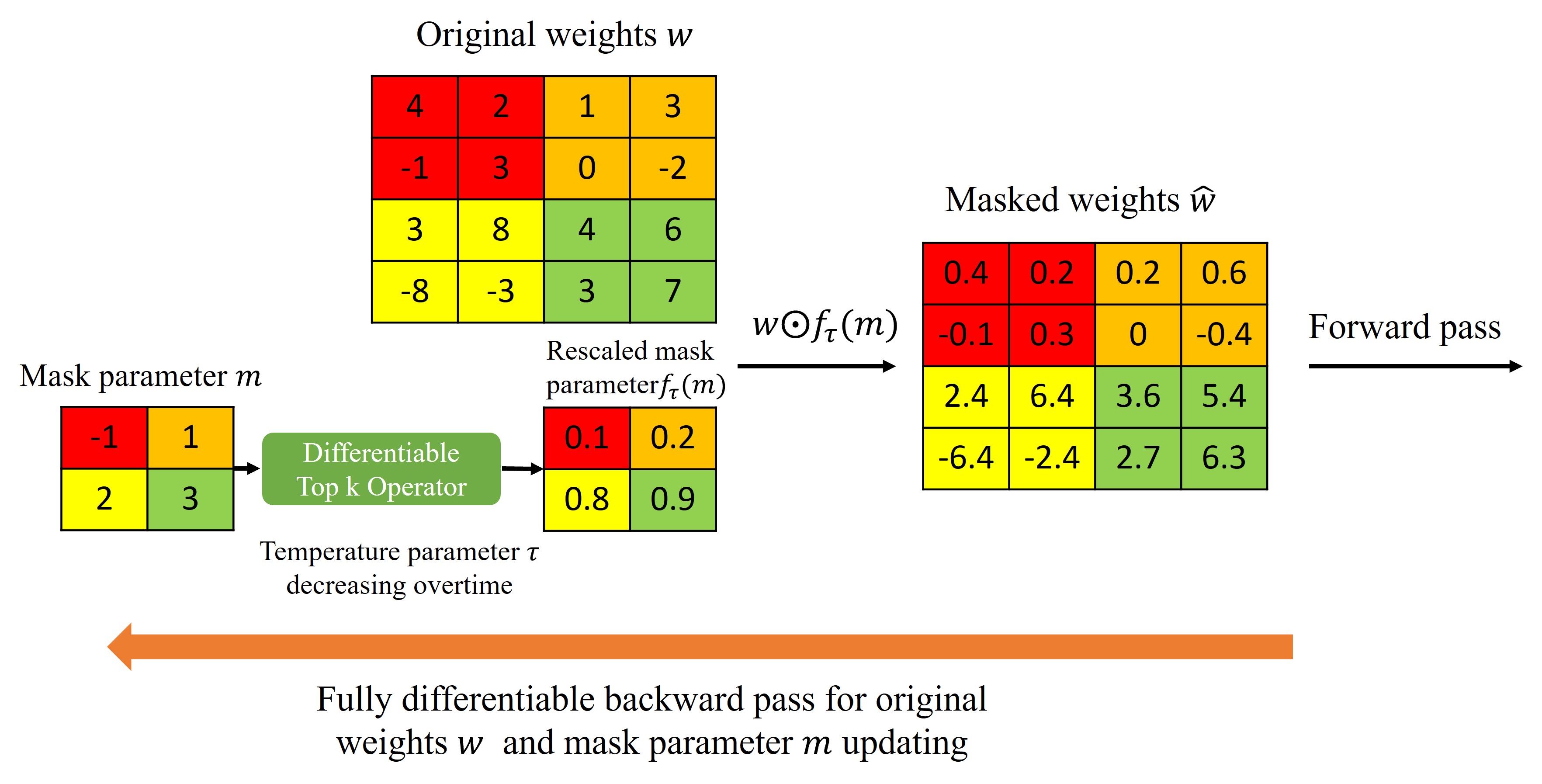
To address these limitations, we propose a novel pruning method – SMART pruning algorithm. To better capture cross-layer dependencies, we rank the weight importance based on a separate learnable soft probability mask. Our target is to train such mask to progressively converge to 0 (to-prune) and 1 (not-to-prune). To facilitate this process, we employ a differentiable Top operator to iteratively adjust and redistribute mask parameters. In our algorithm, the differentiable Top operator could (1) redistribute mask in each iteration to accommodate weight updates. (2) facilitate soft probability mask to converge to binary mask gradually. (3) maintain both forward and backward pass to be differentiable. To avoid non-sparse local minimum before weight freeze, we employ the dynamic temperature parameter trick, which is to change the temperature parameter from high to low gradually during training phases. With higher temperature parameters, the differentiable Top function is smoother, increasing the probability for a mask element to flip from ‘0’ mask to ‘1’ mask. While lower temperature parameters make the differentiable Top function sharper, amplifying the magnitude difference between ‘0’ mask elements and ‘1’ mask elements. By adopting differentiable Top operator with dynamic temperature parameter trick, we could update soft probability mask iteratively and learn the weight importance ranking via backpropagation.
Compared to criteria-based methods, our algorithm integrates importance ranking into training procedure, thereby reducing the probability of pruning out important weight. Compared to weight-frozen learnable pruning masks methods, our approach ensures that the importance masks dynamically adjust to accommodate weight changes. Moreover, our method eliminates the necessity for complicated auxiliary model training, thus more suitable for industrial applications. Compared to STE-based approaches, we counteract the STE learning delay issue by adopting a smooth probability mask. Furthermore, our pruning method eliminates the need for extensive parameter searching and guarantees convergence. Compared to PDP, we mainly have two advantages: (1) Our mask, being directly trainable, eliminates the restrictive presumption that larger magnitude weights are more important across layers. By removing this restrictive assumption, we could better rank the cross-layer weight importance. (2) Our method, utilizing easy-to-tune dynamic temperature parameters, ensures convergence to sparse weight solution without increasing tuning effort. Our major contributions include:
-
•
SMART pruner is the pioneering work in directly training a separate learnable probability mask of weight importance. This innovation enables more precise ranking of cross-layer weight importance and ensures convergence.
-
•
The adoption of dynamic temperature parameter trick enables the pruner to escape from non-sparse local minima, thereby preventing substantial accuracy decreases in some applications.
-
•
Theoretical analysis supports that as temperature parameter approaches zero, the global optimum solution of SMART pruner is equivalent to the global optimum solution of the most fundamental pruning problem, mitigating the impact of regularization bias.
-
•
Experimental studies demonstrate that the SMART pruner achieves state-of-the-art performance on a variety of models and tasks.
2 Methodology
In this section, we will introduce the methodology of SMART pruner. Specifically, in section 2.1, we will introduce our differentiable Top operator, which is the cornerstone of our SMART pruner. Section 2.2 elaborates on the SMART pruning algorithm, including the problem formulation and detailed training flow. Finally, section 2.3 elaborates on our dynamic temperature parameter trick, explaining its role in avoiding non-sparse local minima.
2.1 Differentiable Top Operator
In the deep learning field, the selection of the Top elements is a fundamental operation with extensive applications, ranging from recommendation systems to computer vision (Shazeer et al., 2017; Fedus et al., 2022). Standard Top operators, however, suffer from non-differentiability, which impedes their direct utilization within gradient-based learning frameworks. Typically, the standard Top operator could be written as:
| (1) |
where represents -th input value, refers to the sorted permutations, i.e., .
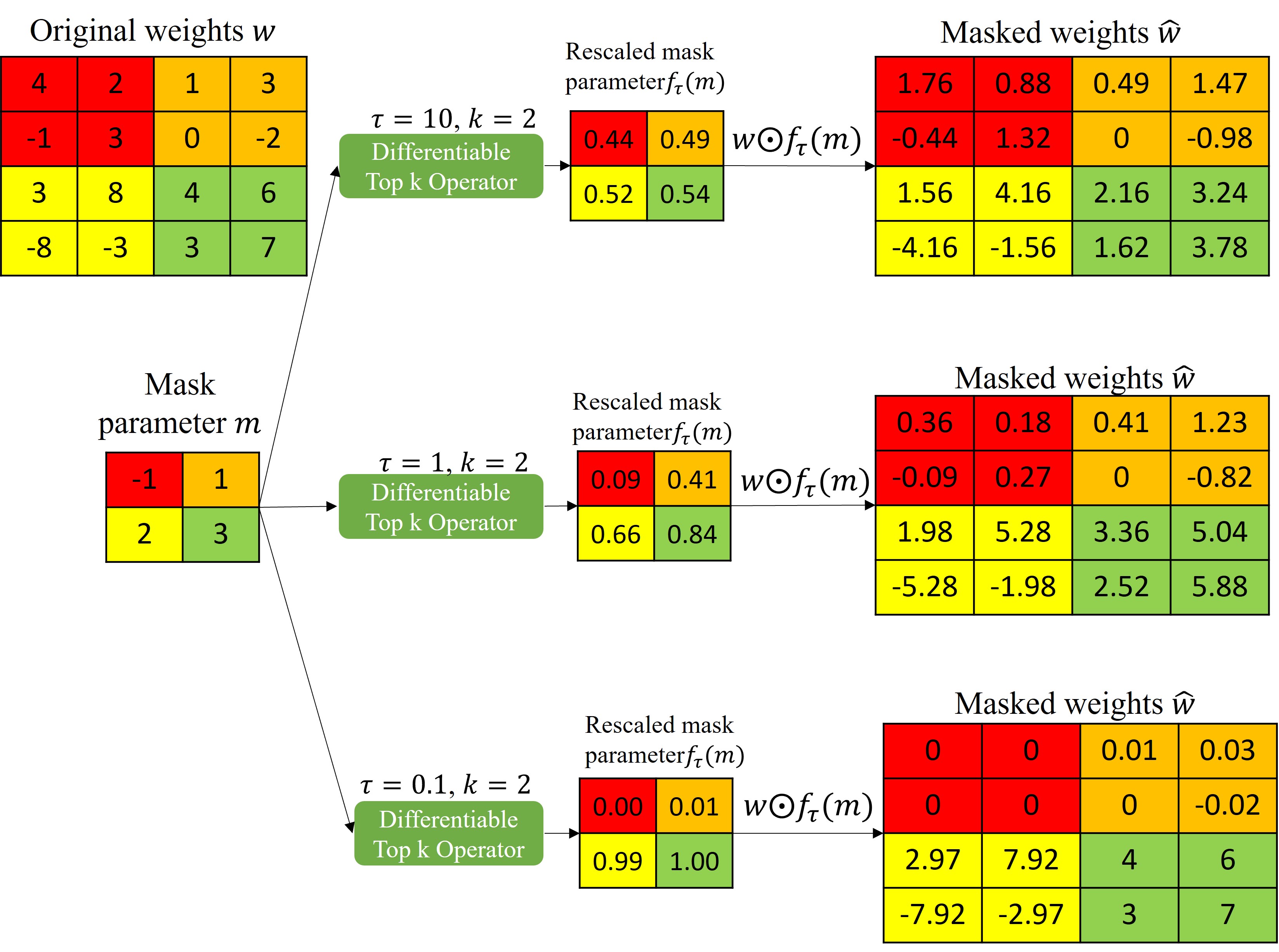
There are numerous works focusing on designing differentiable Top operators (Xie et al., 2020; Sander et al., 2023). Our requirement of differentiable Top operators is (i) simple to implement and (ii) capable of arbitrary precision approximation. To achieve this goal, we modify the sigmoid-based Top operator (Ahle, 2023) by introducing the temperature parameter and the mathematical definition of our differentiable Top operator is as follows:
| (2) | |||
where denotes the total number of inputs, specifies the number of largest elements to be selected by the Top operator, stands for the temperature parameter, and represents the -th input variable. The function represents the sigmoidal activation function, mapping the input into the interval. The determination of hinges on the monotonicity of the sigmoid function. A viable approach to calculate is the binary search algorithm, ensuring that the constraint of Equation (2) is satisfied.
Theorem 2.1.
Suppose and , as the temperature parameter approaches zero, we have , and .
The proof can be found in Appendix A. From Theorem 2.1, we prove that this differentiable Top operator could approximate the standard Top operator to an arbitrary precision by simply reducing the temperature parameter.
Proposition 2.2.
The gradient of is:
where is the gradient of the sigmoid function. The notation is a conditional expression, where it equals 1 if , and 0 otherwise. If we further define , the Jacobian of our differentiable Top-k operator at is:.
The proof of proposition 2.2 can be found in Appendix B. From Proposition 2.2, the backpropagation of this differentiable Top operator could be easily computed. From the above derivation, it is evident that the time and space complexities of both the forward and backward passes are .
2.2 SMART pruning algorithm
Let represent the loss function, denote the weights blocks (grouped by the pruning structure), represent the total number of weights blocks, and indicate the sparsity ratio. A typical pruning problem can be formulated as solving the following optimization problem:
| (3) | ||||
| subject to |
where denotes the zero-norm, which counts the total number of non-zero weight blocks.
Theorem 2.3.
Suppose the pair is the global optimum solution of the following problem (4), then is also the global optimum solution of problem (3).
| (4) | ||||
| subj |
where is the Hadamard product.
The proof of Theorem 2.3 can be found in Appendix C. Theorem 2.3 enables us to shift our focus from solving the problem (3) to solving the problem (4). A significant hurdle in optimizing problem (4) is the non-differentiability of its objective function. To overcome this challenge, we replace the standard Top operator with our differentiable Top operator. We define such that the -th element multiplication . Then, the problem (4) is transformed into the new problem (5), which is the problem formulation for our SMART pruner:
| (5) | |||
Theorem 2.4.
Suppose the pair is the global optimum solution of problem (4) and is a Lipschitz continuous loss function. Then, for any given solution pair satisfying , there exists a such that for any , the inequality holds: .
The proof of Theorem 2.4 can be found in Appendix D. From the Theorem 2.3 and Theorem 2.4, our SMART pruner inherently strives to solve the fundamental pruning problem directly as temperature parameter approaches 0. By directly solving the fundamental pruning problem, our SMART algorithm mitigates the impact of regularization bias, resulting in superior performance over existing arts. During the training procedure, our SMART pruner employs projected stochastic gradient descent to solve the problem (5). The detailed training flow of our SMART pruning algorithm is summarized in Algorithm 1.

In Algorithm 1, denotes the total number of epochs allocated for pretraining, while represents the combined total number of epochs dedicated to both pretraining and structural searching. Additionally, and signify the starting and ending values of the temperature parameter, respectively. Algorithm 1 outlines a three-phase process in our algorithm: (1) The pre-training stage, which focuses on acquiring a pre-trained model; (2) The structural-searching stage, dedicated to identifying the optimal pruning structure; and (3) The fine-tuning stage, aimed at further improving model performance.
The SMART pruning algorithm is also adaptable to N:M pruning scenarios. Detailed information on this extension is provided in Appendix F.
2.3 Dynamic temperature parameter trick
The gradients of the original weights and masks in the SMART pruning algorithm are as follows:
| (6) | ||||
To illustrate the effect of fixed temperature parameters, we introduce Theorem 2.5.
Theorem 2.5.
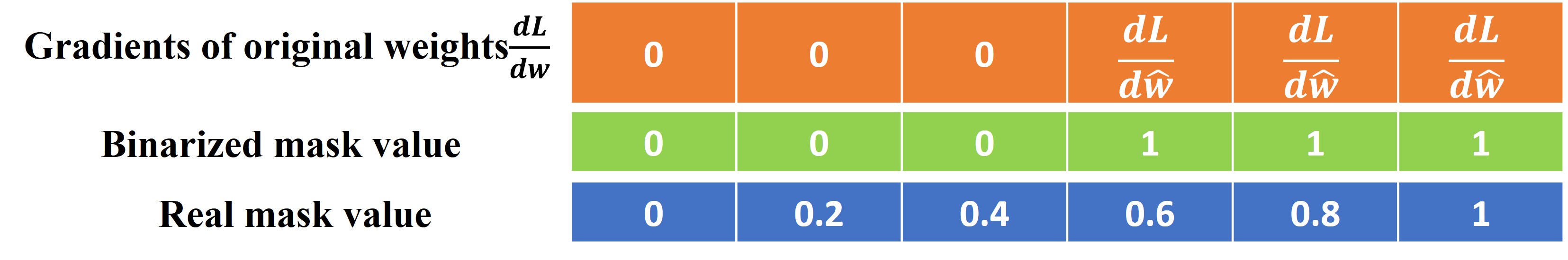
For any given , if the gradients of masked weights equal zero, , then the gradients of original weights and the gradients of mask equals zero.
The proof of Theorem 2.5 is straightforward if the feasible region of is , with representing the total number of weight elements. As shown in the Equation (6), for any , there exists a corresponding set of parameters that satisfies the constraint . This confirms that the feasible region for is indeed , thereby validating Theorem 2.5. This theorem implies that when the temperature parameter is fixed, our algorithm may converge to a non-sparse local minimum prior to weight freeze. This analysis can also be applied to other soft probability mask-based pruning methods, such as PDP, which may similarly result in non-sparse solutions.
To address this challenge, we integrate a dynamic temperature parameter trick in our approach. This technique entails the continual reduction of the temperature parameter within each mini batch during the structural searching phase. To demonstrate the efficacy of the dynamic temperature parameter trick in facilitating the escape from non-sparse local minima, we introduce Proposition 2.6.
Proposition 2.6.
For any given and weights block , we have
The proof of proposition 2.6 is straightforward. It shows that approaches zero if and only if either is close to zero or is close to one. In the non-sparse local minimum case, where neither is close to zero nor is close to one, a significant fluctuation occurs due to temperature reduction, as summarized in Table 1. This fluctuation provides an opportunity to escape the non-sparse local minimum, thereby facilitating the continued convergence towards sparse solutions.
| Masked weights | ||
|---|---|---|
| Mask value | Not close to zero | Close to zero |
| Not close to one | Large | Negligible |
| Close to one | Negligible | Negligible |
In practice, we employ the exponential temperature updating function , with the definitions as follows:
3 Experimental Results
We compare our SMART pruner with state-of-the-art block, output channel, and N:M pruning schemes on various computer vision tasks and models. Motivated by practical applications on a top tier Chinese autonomous driving chip, we make minor modifications to some models for optimal hardware compatibility. All models are trained from scratch. Detailed hyper-parameters are available in Table 5 of Appendix H.
Block pruning for vision benchmark: In our study, we benchmarked the SMART pruning algorithm against the most recent advancements in the field, including PDP, ACDC , PaS and AWG, across three key tasks: classification, object detection, and image segmentation. For classification, we utilized Resnet50 (He et al., 2016) on the ImageNet dataset (Deng et al., 2009). For object detection, Yolov5m (Jocher, 2020) (ReLU version) was chosen for evaluation on the COCO dataset (Lin et al., 2014). For image segmentation, we employed a variant of BiSeNetv2(Yu et al., 2021) on the Cityscapes dataset (Cordts et al., 2015). This adaptation involved replacing the ReduceMean operator with two average pool and one resize operators, a modification specifically designed to ensure compatibility with a leading Chinese autonomous driving chip.
Considering the specific constraints of the real hardware we used, we defined the block shape in our study as 16×8×1×1, where 16 represents the number of output channels, 8 represents the number of input channels, and 1×1 are the conv kernel size dimensions, respectively. To the best of our knowledge, there is no existing research offering tuning parameters for block pruning with this specific block shape. Therefore, we fine-tuned the competing methods as thoroughly as possible to optimize their performance. Detailed settings of hyper-parameters are available in Table 5 in Appendix H. Furthermore, the AWG pruning algorithm is elaborated in detail in Appendix G.
The primary goal of pruning is to balance both model accuracy and latency. For most hardware, sparsity has a greater influence on latency compared to MAC. This is because sparsity not only influences MAC but also impacts the time required to load weights. Therefore, we use sparsity as a proxy for latency, comparing various methods across different levels of sparsity, such as , , .
Our experimental results are summarized in Table 2. In Table 2, we compare our SMART pruner with benchmark methods across three different neural network models: Yolov5m, Resnet50 and BiSeNetv2, evaluated using different metrics. For Yolov5m, the metric used is Mean Average Precision (MAP), while for Resnet50, it is the Top 1 Accuracy, and for BiSeNetv2, the evaluation is based on Mean Intersection over Union (MIOU). The table categorizes the results based on different sparsity levels: , and . The results in Table 2 clearly show that our SMART pruning algorithm outperforms all benchmark methods at each sparsity level, consistently across all the models evaluated.
| Sparsity | Method | Yolov5m (MAP) | Resnet50 (Top-1 Acc) | BiSeNetv2 (MIOU) |
|---|---|---|---|---|
| Original | - | 0.426 | 0.803 | 0.725 |
| 30% | SMART | 0.423 | 0.798 | 0.738 |
| PDP | 0.401 | 0.796 | 0.734 | |
| PaS | 0.416 | 0.795 | 0.731 | |
| AWG | 0.404 | 0.793 | 0.734 | |
| ACDC | 0.403 | 0.795 | 0.732 | |
| 50% | SMART | 0.416 | 0.790 | 0.735 |
| PDP | 0.384 | 0.787 | 0.731 | |
| PaS | 0.407 | 0.784 | 0.727 | |
| AWG | 0.392 | 0.781 | 0.733 | |
| ACDC | 0.379 | 0.785 | 0.727 | |
| 70% | SMART | 0.400 | 0.775 | 0.721 |
| PDP | 0.323 | 0.758 | 0.702 | |
| PaS | 0.377 | 0.761 | 0.689 | |
| AWG | 0.355 | 0.758 | 0.699 | |
| ACDC | 0.318 | 0.759 | 0.691 |
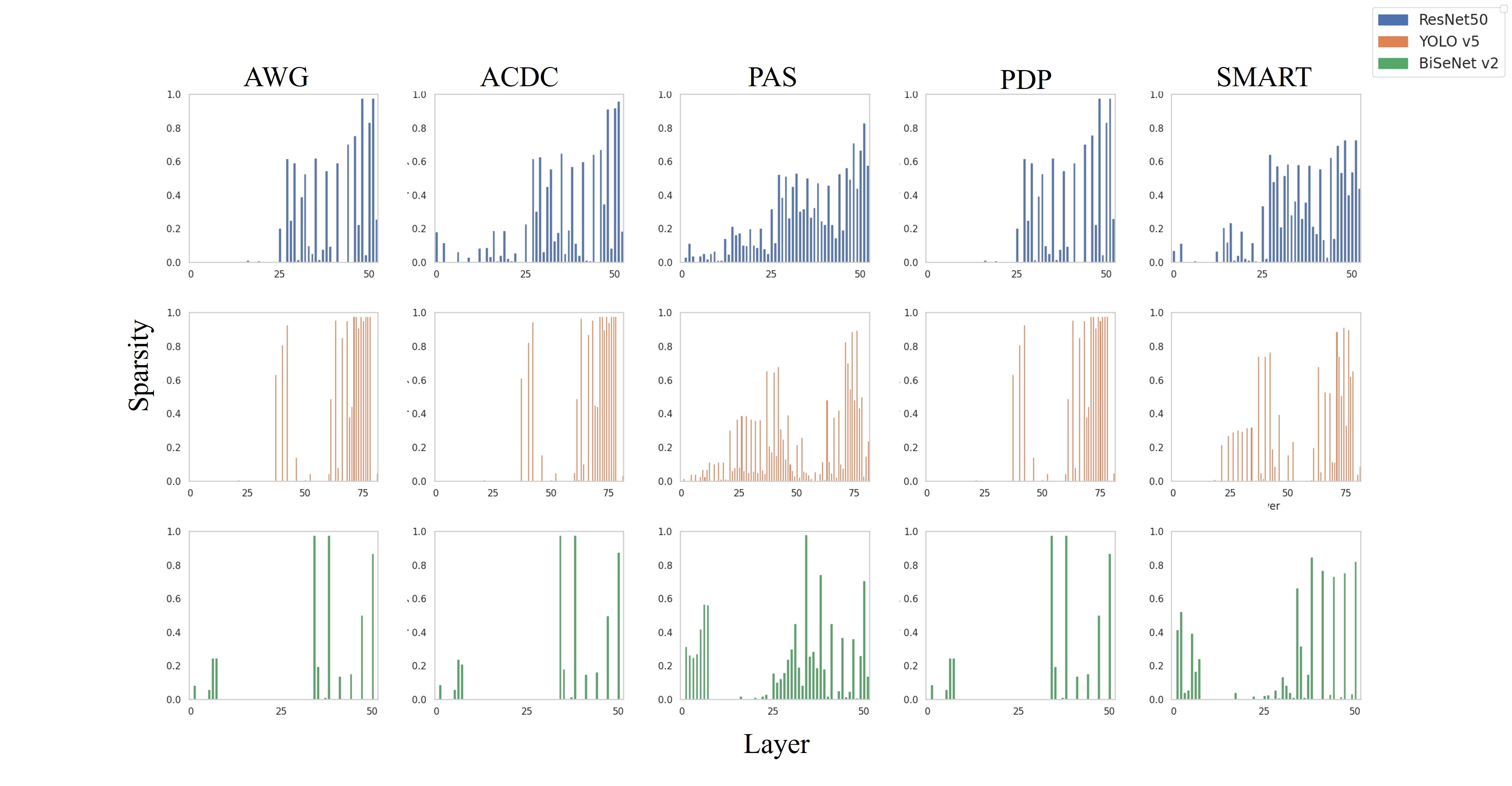
As depicted in Figure 4, the SMART pruner exhibits significantly distinct layer-wise sparsity patterns compared to other pruning algorithms. This notable difference suggests that the training flow of the SMART pruner influences the cross-layer sparsity distribution, potentially contributing to its superior performance.
Output channel pruning for vision benchmark: Output channel pruning, which involves eliminating entire output channels, typically yields the worst accuracy among structural pruning methods at equivalent sparsity levels due to its larger granularity. However, its advantages are notable: (1) it is the only pruning method that reduces data I/O. (2) it could achieve hardware-agnostic acceleration, meaning it can enhance performance on any hardware without requirement of specific hardware designs. In contrast, both block and N:M pruning necessitate specialized hardware designs to realize actual performance gains. In our output channel pruning study, we compared the five pruning methods – SMART, PDP, PaS, AWG, and ACDC – across the three models: Yolov5m, Resnet50, and BiSeNetv2. This comparison was conducted at an output channel sparsity level of and . The results shown in Table 3 clearly demonstrate the superior effectiveness of the SMART pruning algorithm over existing methods in the context of output channel pruning.
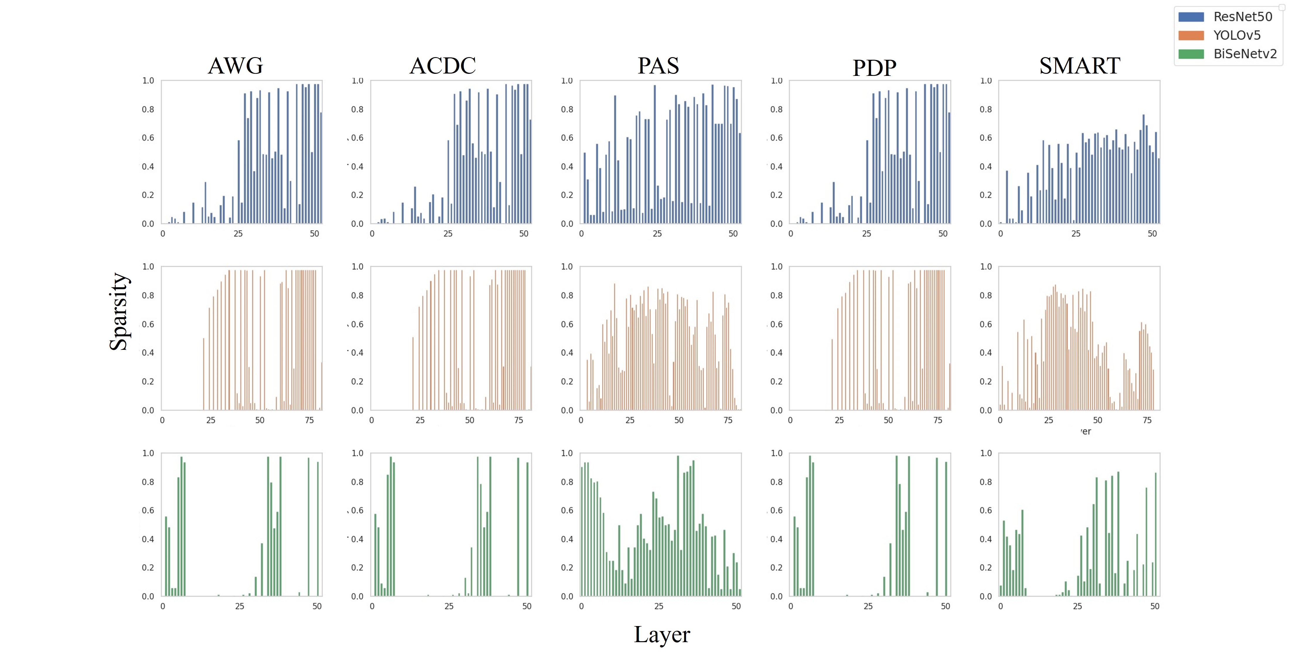
Figure 5 demonstrates that the SMART pruner exhibits significant difference in layer-wise sparsity compared to other algorithms. With the larger granularity of output channel pruning, cross-layer sparsity becomes more critical to final accuracy. Therefore, the superior ranking in cross-layer sparsity could be the key factor in the substantial outperformance of the SMART pruner over other benchmarks.
| Sparsity | Method | Yolov5m (MAP) | Resnet50 (Top-1 Acc) | BiSeNetv2 (MIOU) |
|---|---|---|---|---|
| Original | - | 0.426 | 0.803 | 0.725 |
| 20% | SMART | 0.414 | 0.789 | 0.737 |
| PDP | 0.307 | 0.776 | 0.736 | |
| PaS | 0.384 | 0.779 | 0.703 | |
| AWG | 0.308 | 0.781 | 0.734 | |
| ACDC | 0.303 | 0.777 | 0.688 | |
| 50% | SMART | 0.331 | 0.747 | 0.720 |
| PDP | 0.115 | 0.636 | 0.682 | |
| PaS | 0.310 | 0.555 | 0.311 | |
| AWG | 0.124 | 0.661 | 0.701 | |
| ACDC | 0.110 | 0.615 | 0.685 |
N:M pruning for vision benchmark: While our algorithm was initially developed with a focus on block/output channel pruning for CNN models, we were keen to assess its performance on N:M pruning with Transformer-based models. Therefore, we applied the same suite of five pruning algorithms, including our SMART pruning method, to both the Swin Transformer (Liu et al., 2021b) and the Vision Transformer (ViT) (Dosovitskiy et al., 2020), specifically using a 2:4 pruning ratio. The performance metric of these models is Top 1 accuracy, and the results are summarized in Table 4. From these results, it is evident that our SMART pruning algorithm also performs commendably on Transformer-based models in the context of N:M pruning. This demonstrates the algorithm’s versatility and robustness, extending its applicability beyond CNN architectures to include Transformer-based models.
| Sparsity | Method | Swin-Transformer (Top-1 Acc) | Vision-Transformer (Top-1 Acc) |
|---|---|---|---|
| Original | - | 0.813 | 0.788 |
| 2:4 | SMART | 0.805 | 0.768 |
| PDP | 0.805 | 0.765 | |
| PaS | 0.794 | 0.765 | |
| AWG | 0.797 | 0.764 | |
| ACDC | 0.798 | 0.761 |
4 Conclusion
In this paper, we propose a novel SMART pruner to improve the block/output channel pruning. SMART pruner ranks the weight importance based on a separate, directly learnable probability mask to better capture the cross-layer correlation. Additionally, the dynamic temperature parameter trick aids in overcoming non-sparse local minima, further enhancing the pruner’s effectiveness. Empirical studies have confirmed that our SMART pruner outperforms existing methods in a wide range of computer vision tasks and models, specifically in block and output channel pruning. Moreover, the SMART pruner has also demonstrated its superiority in N:M pruning for Transformer-based models, showcasing its adaptability and robustness.
References
- Ahle (2023) Ahle, T. Differentiable Top-k function. https://math.stackexchange.com/questions/3280757/differentiable-top-k-function, 2023. Accessed: 2024-01-12.
- Anasosalu Vasu et al. (2022) Anasosalu Vasu, P. K., Gabriel, J., Zhu, J., Tuzel, O., and Ranjan, A. MobileOne: An improved one millisecond mobile backbone. arXiv e-prints, pp. arXiv–2206, 2022.
- Cho et al. (2021) Cho, M., Vahid, K. A., Adya, S., and Rastegari, M. Dkm: Differentiable k-means clustering layer for neural network compression. arXiv preprint arXiv:2108.12659, 2021.
- Cho et al. (2023) Cho, M., Adya, S., and Naik, D. PDP: Parameter-free Differentiable Pruning is all you need. arXiv preprint arXiv:2305.11203, 2023.
- Cordts et al. (2015) Cordts, M., Omran, M., Ramos, S., Scharwächter, T., Enzweiler, M., Benenson, R., Franke, U., Roth, S., and Schiele, B. The cityscapes dataset. In CVPR Workshop on the Future of Datasets in Vision, volume 2. sn, 2015.
- Deng et al. (2009) Deng, J., Dong, W., Socher, R., Li, L.-J., Li, K., and Fei-Fei, L. Imagenet: A large-scale hierarchical image database. In 2009 IEEE conference on computer vision and pattern recognition, pp. 248–255. IEEE, 2009.
- Dosovitskiy et al. (2020) Dosovitskiy, A., Beyer, L., Kolesnikov, A., Weissenborn, D., Zhai, X., Unterthiner, T., Dehghani, M., Minderer, M., Heigold, G., Gelly, S., et al. An image is worth 16x16 words: Transformers for image recognition at scale. arXiv preprint arXiv:2010.11929, 2020.
- Fedus et al. (2022) Fedus, W., Dean, J., and Zoph, B. A review of sparse expert models in deep learning. arXiv preprint arXiv:2209.01667, 2022.
- Gao et al. (2022) Gao, S., Huang, F., Zhang, Y., and Huang, H. Disentangled differentiable network pruning. In European Conference on Computer Vision, pp. 328–345. Springer, 2022.
- Han et al. (2015a) Han, S., Mao, H., and Dally, W. J. Deep compression: Compressing deep neural networks with pruning, trained quantization and huffman coding. arXiv preprint arXiv:1510.00149, 2015a.
- Han et al. (2015b) Han, S., Pool, J., Tran, J., and Dally, W. Learning both weights and connections for efficient neural network. Advances in neural information processing systems, 28, 2015b.
- He et al. (2016) He, K., Zhang, X., Ren, S., and Sun, J. Deep residual learning for image recognition. In Proceedings of the IEEE conference on computer vision and pattern recognition, pp. 770–778, 2016.
- He et al. (2017) He, Y., Zhang, X., and Sun, J. Channel pruning for accelerating very deep neural networks. In Proceedings of the IEEE international conference on computer vision, pp. 1389–1397, 2017.
- He et al. (2018) He, Y., Lin, J., Liu, Z., Wang, H., Li, L.-J., and Han, S. AMC: Automl for model compression and acceleration on mobile devices. In Proceedings of the European conference on computer vision (ECCV), pp. 784–800, 2018.
- Howard et al. (2017) Howard, A. G., Zhu, M., Chen, B., Kalenichenko, D., Wang, W., Weyand, T., Andreetto, M., and Adam, H. MobileNets: Efficient convolutional neural networks for mobile vision applications. arXiv preprint arXiv:1704.04861, 2017.
- Jocher (2020) Jocher, G. YOLOv5 by Ultralytics, May 2020. URL https://github.com/ultralytics/yolov5.
- Kusupati et al. (2020) Kusupati, A., Ramanujan, V., Somani, R., Wortsman, M., Jain, P., Kakade, S., and Farhadi, A. Soft threshold weight reparameterization for learnable sparsity. In International Conference on Machine Learning, pp. 5544–5555. PMLR, 2020.
- Lagunas et al. (2021) Lagunas, F., Charlaix, E., Sanh, V., and Rush, A. M. Block pruning for faster transformers. arXiv preprint arXiv:2109.04838, 2021.
- Lee et al. (2021) Lee, J., Kim, D., and Ham, B. Network quantization with element-wise gradient scaling. In Proceedings of the IEEE/CVF conference on computer vision and pattern recognition, pp. 6448–6457, 2021.
- Li et al. (2019) Li, Y., Dong, X., and Wang, W. Additive powers-of-two quantization: An efficient non-uniform discretization for neural networks. arXiv preprint arXiv:1909.13144, 2019.
- Li et al. (2022) Li, Y., Zhao, P., Yuan, G., Lin, X., Wang, Y., and Chen, X. Pruning-as-search: Efficient neural architecture search via channel pruning and structural reparameterization. arXiv preprint arXiv:2206.01198, 2022.
- Lin et al. (2020) Lin, M., Ji, R., Zhang, Y., Zhang, B., Wu, Y., and Tian, Y. Channel pruning via automatic structure search. arXiv preprint arXiv:2001.08565, 2020.
- Lin et al. (2014) Lin, T.-Y., Maire, M., Belongie, S., Hays, J., Perona, P., Ramanan, D., Dollár, P., and Zitnick, C. L. Microsoft coco: Common objects in context. In Computer Vision–ECCV 2014: 13th European Conference, Zurich, Switzerland, September 6-12, 2014, Proceedings, Part V 13, pp. 740–755. Springer, 2014.
- Liu et al. (2021a) Liu, S., Chen, T., Chen, X., Atashgahi, Z., Yin, L., Kou, H., Shen, L., Pechenizkiy, M., Wang, Z., and Mocanu, D. C. Sparse training via boosting pruning plasticity with neuroregeneration. Advances in Neural Information Processing Systems, 34:9908–9922, 2021a.
- Liu et al. (2021b) Liu, Z., Lin, Y., Cao, Y., Hu, H., Wei, Y., Zhang, Z., Lin, S., and Guo, B. Swin transformer: Hierarchical vision Transformer using shifted windows. In Proceedings of the IEEE/CVF international conference on computer vision, pp. 10012–10022, 2021b.
- Mehta & Rastegari (2021) Mehta, S. and Rastegari, M. MobileVIT: light-weight, general-purpose, and mobile-friendly vision Transformer. arXiv preprint arXiv:2110.02178, 2021.
- Peste et al. (2021) Peste, A., Iofinova, E., Vladu, A., and Alistarh, D. Ac/dc: Alternating compressed/decompressed training of deep neural networks. Advances in neural information processing systems, 34:8557–8570, 2021.
- Polino et al. (2018) Polino, A., Pascanu, R., and Alistarh, D. Model compression via distillation and quantization. arXiv preprint arXiv:1802.05668, 2018.
- Reed (1993) Reed, R. Pruning algorithms-a survey. IEEE transactions on Neural Networks, 4(5):740–747, 1993.
- Sander et al. (2023) Sander, M. E., Puigcerver, J., Djolonga, J., Peyré, G., and Blondel, M. Fast, differentiable and sparse Top-k: a convex analysis perspective. In International Conference on Machine Learning, pp. 29919–29936. PMLR, 2023.
- Sandler et al. (2018) Sandler, M., Howard, A., Zhu, M., Zhmoginov, A., and Chen, L.-C. MobileNetv2: Inverted residuals and linear bottlenecks. In Proceedings of the IEEE conference on computer vision and pattern recognition, pp. 4510–4520, 2018.
- Sanh et al. (2020) Sanh, V., Wolf, T., and Rush, A. Movement pruning: Adaptive sparsity by fine-tuning. Advances in Neural Information Processing Systems, 33:20378–20389, 2020.
- Shazeer et al. (2017) Shazeer, N., Mirhoseini, A., Maziarz, K., Davis, A., Le, Q., Hinton, G., and Dean, J. Outrageously large neural networks: The sparsely-gated mixture-of-experts layer. arXiv preprint arXiv:1701.06538, 2017.
- Silver et al. (2018) Silver, D., Hubert, T., Schrittwieser, J., Antonoglou, I., Lai, M., Guez, A., Lanctot, M., Sifre, L., Kumaran, D., Graepel, T., et al. A general reinforcement learning algorithm that masters chess, shogi, and Go through self-play. Science, 362(6419):1140–1144, 2018.
- Sun et al. (2021) Sun, W., Zhou, A., Stuijk, S., Wijnhoven, R., Nelson, A. O., Corporaal, H., et al. Dominosearch: Find layer-wise fine-grained N:M sparse schemes from dense neural networks. Advances in neural information processing systems, 34:20721–20732, 2021.
- Unlu (2020) Unlu, H. Efficient neural network deployment for microcontroller. arXiv preprint arXiv:2007.01348, 2020.
- Van Delm et al. (2023) Van Delm, J., Vandersteegen, M., Burrello, A., Sarda, G. M., Conti, F., Pagliari, D. J., Benini, L., and Verhelst, M. HTVM: Efficient neural network deployment on heterogeneous TinyML platforms. In 2023 60th ACM/IEEE Design Automation Conference (DAC), pp. 1–6. IEEE, 2023.
- Wang et al. (2019) Wang, K., Liu, Z., Lin, Y., Lin, J., and Han, S. Haq: Hardware-aware automated quantization with mixed precision. In Proceedings of the IEEE/CVF conference on computer vision and pattern recognition, pp. 8612–8620, 2019.
- Wortsman et al. (2019) Wortsman, M., Farhadi, A., and Rastegari, M. Discovering neural wirings. Advances in Neural Information Processing Systems, 32, 2019.
- Wu et al. (2018) Wu, J., Wang, Y., Wu, Z., Wang, Z., Veeraraghavan, A., and Lin, Y. Deep k-means: Re-training and parameter sharing with harder cluster assignments for compressing deep convolutions. In International Conference on Machine Learning, pp. 5363–5372. PMLR, 2018.
- Xie et al. (2020) Xie, Y., Dai, H., Chen, M., Dai, B., Zhao, T., Zha, H., Wei, W., and Pfister, T. Differentiable Top-k with optimal transport. Advances in Neural Information Processing Systems, 33:20520–20531, 2020.
- Yu et al. (2021) Yu, C., Gao, C., Wang, J., Yu, G., Shen, C., and Sang, N. BiSeNet v2: Bilateral network with guided aggregation for real-time semantic segmentation. International Journal of Computer Vision, 129:3051–3068, 2021.
- Zafrir et al. (2021) Zafrir, O., Larey, A., Boudoukh, G., Shen, H., and Wasserblat, M. Prune once for all: Sparse pre-trained language models. arXiv preprint arXiv:2111.05754, 2021.
- Zhang et al. (2022) Zhang, Y., Lin, M., Chen, M., Xu, Z., Chao, F., Shen, Y., Li, K., Wu, Y., and Ji, R. OptG: Optimizing Gradient-driven criteria in network sparsity. arXiv preprint arXiv:2201.12826, 2022.
- Zhao et al. (2019) Zhao, X., Wang, Y., Cai, X., Liu, C., and Zhang, L. Linear symmetric quantization of neural networks for low-precision integer hardware. In International Conference on Learning Representations, 2019.
- Zhu & Gupta (2017) Zhu, M. and Gupta, S. To prune, or not to prune: exploring the efficacy of pruning for model compression. arXiv preprint arXiv:1710.01878, 2017.
Appendix A Proof of Theorem 2.1
Proof.
Given the monotonicity of the sigmoid function, we have . We prove Theorem 2.1 by contradiction.
Define: , we have (1) , (2) , (3) .
Suppose , where , we have: . Define , we have: . Given the monotonicity of the sigmoid function, we have: , which is a contradict. Thus, .
Similarly, suppose , where , we have: . Define , we have: . Given the monotonicity of the sigmoid function, we have:
, which is a contradict. Thus, .
∎
Appendix B Proof of Proposition 2.2
Proof.
The gradient of can be calculated as follows:
| (7) |
To obtain the gradient of , we need to determine . To determine the value of , we employ a methodology like the one described in (Ahle, 2023). Specifically, the steps for derivation are outlined as follows:
| (8) |
Then we have:
| (9) |
By plugging Equation (9) into Equation (8), we obtain the following result:
| (10) |
Then, by defining , it follows directly from Equation (10) that . ∎
Appendix C Proof of Theorem 2.3
Proof.
We proceed with a proof by contradiction. Assume the existence of a vector such that , subject to sparsity constraint . Let us define and , we have , which contradicts the premise that the pair is the global optimum solution. ∎
Appendix D Proof of Theorem 2.4
Proof.
Suppose is the Lipschitz constant of loss function , and define , we have:
Since is a Lipschitz continuous function with Lipschitz constant , we have:
Then we have:
Theorem 2.1 shows that the differentiable Top k function can approximate the standard Top k function with arbitrary precision. Thus, there exists a such that for any , we have:
This inequality implies:
∎
Appendix E Illustration of STE Learning Delay Issue
The loss function employed in typical STE-based methods can be mathematically formulated as follows:
| (11) |
In this expression, represents the rounding operator, which rounds the values of to lie within the range of 0 and 1. The denotes the regularization term. The parameter is a tuning parameter, which balances between the primary loss function and the regularization term. The gradients of (11) are as follows:
| (12) | ||||
| (13) | ||||
| subject to |
In Equation (13), the symbol represents a typical approximation used in STE methods. From Equation (12), we observe that when , the derivative of the loss function with respect to the weights, , consistently equals zero. Conversely, when , the derivative becomes equivalent to . Such behavior suggests that variations in the mask value have no effect on the weight parameters until there is a definitive switch in the mask value from 0 to 1, or vice versa. This delayed awareness can, however, lead to significant accuracy drops and stability issues in certain applications.
Appendix F Extension to N:M pruning
While our SMART pruning algorithm was originally designed for block and output channel pruning, it is applicable to N:M pruning with some modifications. The modifications are required due to differences between N:M pruning and block/output channel pruning. Firstly, unlike block or output channel pruning, N:M pruning does not involve issues related to cross-layer sparsity distribution. Secondly, as N:M pruning is a fine-grained technique, the usage of an importance mask in this context would lead to a mask size that is comparable to the size of the weights. Thus, to suit N:M pruning, we revised our original problem formulation presented in Equation (5). This revision, as shown in the Equation (14), removes the importance mask parameters:
| (14) | ||||
Here, denotes the differentiable Top operator applied to -th weight within weights group . The parameters N and M define the pruning ratio, with N:M indicating that N weights are retained out of every M weights in the group. Additionally, is used to denote the ceiling operator.
With the problem formulation (14), we have accordingly modified our training flow, as illustrated in Algorithm 2. The primary distinction between Algorithm 1 and Algorithm 2 lies in the removal of importance mask parameters.
By eliminating the importance mask parameters, our SMART pruning algorithm now closely aligns with the PDP algorithm, differing in only two aspects. Firstly, we utilize a soft top-k operator to generate the probability mask, while they use SoftMax. Secondly, our approach adopts a dynamic temperature parameter trick, while the PDP algorithm employs fixed temperature parameters. Experimental studies have shown that, in N:M pruning tasks, our SMART pruning algorithm still outperforms the PDP algorithm, although with a relatively small margin.
Appendix G The Accumulated Weight and Gradient (AWG) Pruning Algorithm
The Accumulated Weight and Gradient pruner is an advanced variant of the magnitude-based pruning method, where the importance score is a function of the pre-trained weights and the tracked gradients over one epoch of gradient calibration. As opposed to the pre-trained weights, the product of pre-trained weights and accumulated gradients is assumed to be the proxy for importance. For each layer, the importance score is the product of three terms. 1) The pre-trained weight. 2) The accumulated gradient. 3) The scaling factor, which rescales the importance by favoring (higher score) layers with high sparsity already.
The pruning consists of three stages. 1) Initially, the training data is fed to the pre-trained model and we keep track of the smoothed importance scores via exponential moving average (EMA) at each layer. For more detail regarding how the importance score is computed and updated, please refer to Algorithm 3. Weights are not updated at this stage. After running one epoch, we reduce the importance scores by block and rank them in the ascending order. We prune the least important of the blocks through 0-1 masks. 2) With the masks updated, we fine-tune the weights on the training set for epochs. The masks are kept unchanged throughout the fine-tuning. Typically, we carry out iterative pruning to allow for smoother growth in sparsity and thus more stable convergence, so stages 1 and 2 alternate for steps. 3) At the very last step, we fine-tune the model for another epochs.
A brief explanation for the notation in the algorithm: is the number of iterative steps in pruning. is the decay factor that governs the EMA smoothing for importance. is the number of epochs to fine-tune the model at each iterative step. is the number of epochs to fine-tune the model after the last iterative step is complete. , and are the block-wise weight, mask and EMA importance of the -th block, respectively.
Appendix H Hyperparameter Settings
| Network | Method | Batch size | Epochs | #WU | Main optimizer; scheduler | Mask optimizer; scheduler | Pruning-specific params |
|---|---|---|---|---|---|---|---|
| ResNet50 | AWG | 128 | 100 | 0 | AdamW: 1e-4, 0.9, 0.025; cosine | N/A | mspl: 0.98 |
| ACDC | 256 | 100 | 0 | AdamW: 1e-4, 0.9, 0.025; cosine | N/A | mspl: 0.98, steps: 8, #comp: 5, #decomp: 5 | |
| PAS | 128 | 100 | 0 | AdamW: 1e-5, 0.9, 0.025; cosine | Same as the main | - | |
| PDP | 256 | 100 | 0 | AdamW: 1e-5, 0.9, 0.025; cosine | Same as the main | #se: 20 | |
| Ours | 256 | 100 | 0 | AdamW: 1e-4, 0.9, 0.025; cosine | Same as the main | init_temp: 10, final_temp: 1e-4, #se: 20 | |
| YOLO v5 | AWG | 16 | 100 | 3 | SGD: 1e-4, 0.937, 5e-4; lambdaLR | N/A | mspl: 0.98 |
| ACDC | 32 | 100 | 0 | SGD: 1e-4, 0.937, 5e-4; lambdaLR | N/A | mspl: 0.98, steps: 8, #comp: 5, #decomp: 5 | |
| PAS | 16 | 100 | 3 | SGD: 1e-4, 0.9, 5e-4; lambdaLR | SGD: 1e-3, 0.9, 5e-4, lambdaLR | - | |
| PDP | 32 | 100 | 0 | SGD: 1e-4, 0.937, 5e-4; lambdaLR | Same as the main | #se: 20 | |
| Ours | 16 | 100 | 3 | SGD: 1e-4, 0.937, 5e-4; lambdaLR | Same as the main | init_temp: 10, final_temp: 1e-4, #se: 20 | |
| BiSeNet v2 | AWG | 16 | 134.6 | 0 | SGD: 5e-4, 0.9, 0; WarmupPolyLR | N/A | mspl: 0.98 |
| ACDC | 16 | 134.6 | 0 | SGD: 5e-4, 0.9, 0; WarmupPolyLR | N/A | mspl: 0.98, steps: 8, #comp: 6.73, #decomp: 6.73 | |
| PAS | 16 | 134.6 | 0 | SGD: 5e-4, 0.9, 0; WarmupPolyLR | Same as the main | - | |
| PDP | 16 | 134.6 | 0 | SGD: 5e-4, 0.9, 0; WarmupPolyLR | Same as the main | #se: 62.2 | |
| Ours | 16 | 134.6 | 0 | SGD: 5e-4, 0.9, 0; WarmupPolyLR | SGD: 1e-4, 0.9, 0; WarmupPolyLR | init_temp: 10, final_temp: 1e-4, #se: 9.42 | |
| ViT | AWG | 64 | 150 | 0 | AdamW: 1e-5, 0.9, 0.3; cosine | N/A | - |
| ACDC | 64 | 150 | 0 | AdamW: 1e-5, 0.9, 0.3; cosine | N/A | steps: 2, #comp: 1, #decomp: 1 | |
| PAS | 64 | 150 | 0 | AdamW: 1e-5, 0.9, 0.3; cosine | Same as the main | - | |
| PDP | 64 | 150 | 0 | AdamW: 1e-5, 0.9, 0.3; cosine | Same as the main | #se: 20 | |
| Ours | 64 | 150 | 0 | AdamW: 1e-5, 0.9, 0.3; cosine | Same as the main | init_temp: 1e-4, final_temp: 1e-5, #se: 5 | |
| Swin-Transformer | AWG | 128 | 200 | 20 | AdamW: 5e-6, 0.9, 0.05; cosine | N/A | steps: 5, #feps: 5 |
| ACDC | 128 | 200 | 20 | AdamW: 5e-6, 0.9, 0.05; cosine | N/A | wteps: 5, #comp: 2, #decomp: 2 | |
| PAS | 128 | 200 | 20 | AdamW: 5e-6, 0.9, 0.05; cosine | Same as the main | - | |
| PDP | 128 | 200 | 20 | AdamW: 5e-6, 0.9, 0.05; cosine | Same as the main | #se: 20 | |
| Ours | 128 | 200 | 20 | AdamW: 5e-6, 0.9, 0.05; cosine | Same as the main | init_temp: 10, final_temp: 1e-5, #se: 20 |
Notes:
-
•
#WU means the number of warmup epochs.
-
•
For each pruning method, the same hyperparameter setting was used among all sparsity levels and pruning structures.
Optimizer Parameters:
-
•
SGD: lr, momentum, weight_decay
-
•
AdamW: lr, momentum, weight_decay
Pruning Parameters:
-
•
AWG: mspl = maximum sparsity per layer, steps = iterative steps, #feps = number of fine-tuning epochs per step
-
•
ACDC: mspl = maximum sparsity per layer, steps = iterative steps, #comp = number of compressed epochs per step, #decomp = number of decompressed epochs per step
-
•
PDP: #se = number of search epochs
-
•
Ours (SMART): init_temp = initial temperature, final_temp = final temperature, #se = number of search epochs