Multi-task Magnetic Resonance Imaging Reconstruction using Meta-learning

Abstract

Using single-task deep learning methods to reconstruct Magnetic Resonance Imaging (MRI) data acquired with different imaging sequences is inherently challenging. The trained deep learning model typically lacks generalizability, and the dissimilarity among image datasets with different types of contrast leads to suboptimal learning performance. This paper proposes a meta-learning approach to efficiently learn image features from multiple MR image datasets. Our algorithm can perform multi-task learning to simultaneously reconstruct MR images acquired using different imaging sequences with different image contrasts. The experiment results demonstrate the ability of our new meta-learning reconstruction method to successfully reconstruct highly-undersampled k-space data from multiple MRI datasets simultaneously, outperforming other compelling reconstruction methods previously developed for single-task learning.

1 Introduction

MR images acquired using different imaging sequences can provide complementary soft tissue contrasts, which are collectively used for clinical disease diagnosis. However, MRI is a slow imaging modality, resulting in a high sensitivity to subject motion. Long acquisition time is also undesirable, as it leads to lower patient throughput than other popular imaging modalities. Accelerated MRI acquisition and reconstruction are highly desirable and remain an active research topic [16, 6, 14, 10, 11, 12]. In the past years, deep learning methods [8] have shown great potential to enable rapid MRI. Deep learning approaches typically use task-specific deep networks to learn image features associated with incomplete k-space sampling and aim to remove image artifacts and noises caused by k-space undersampling during accelerated acquisition. While the conventional single-task models can work well when the training and testing data stem from the same data distribution (e.g., acquired using the same imaging sequence), they typically underperform when training and testing data differ substantially (e.g., acquired from different imaging sequences) [1, 15, 9]. Therefore, multi-task deep learning using methods to synergistically learn image features across multiple image datasets with different image contrasts is highly desirable for robust and high-efficient reconstruction.

This paper proposes a meta-learning framework to learn image features from multiple MR image datasets. Meta-learning is a stacking ensemble learning [4] scheme that is considered a process of “learning-to-learn”, which can learn to improve the learning algorithm and parameter generalizability over multiple training episodes, thus enabling each task to learn better [7]. In this study, we developed a bi-level meta-learning reconstruction framework (i.e., including base-level and meta-level) to handle the learning of multiple image datasets. At the base-level, we introduce new deep networks (e.g., base-learners) by unrolling proximal gradient descent in both image and k-space domains to cross-learn the image and frequency domain features for single image contrast. In the meta-level, we introduce an optimization algorithm that can alternatively optimize the base-learners and one additional meta-learner for efficiently characterizing mutual correlation among multiple image datasets. Our bi-level meta-learning can simultaneously reconstruct highly-undersampled k-space data acquired using different imaging sequences with an optimal reconstruction for all image contrasts.

Our contribution can be summarized as follows:
1. A novel bi-level meta-learning framework is proposed to reconstruct highly-undersampled MRI datasets acquired using different imaging sequences.
2. An unrolled network is proposed to extend proximal gradient descent [13] on both image and k-space domains, enabling cross-domain learning of MRI data and leading to a superior reconstruction performance for every single contrast.
3. The proposed algorithm is validated for reconstructing a set of knee MRIs acquired at different imaging contrasts and planes.

2 Methodology and Algorithm

Considering the multi-coil MR images at multi-task image datasets, we denote each image as $\mathbf{x}_{i,j}\in\mathbb{C}^{n}$ for $i=1,\cdots,m$ and $j=1,\cdots,c$, where $m$ is the number of tasks (i.e., the acquired image sequences), $c$ is the number of receiving coils and $n$ is the number of pixels in the image. The corresponding undersampled k-space data can be formulated as $\mathbf{f}_{i,j}=\mathbf{P}\mathbf{F}\mathbf{x}_{i,j}+\mathbf{n}_{i,j}$, where $\mathbf{F}$ denotes the MR encoding matrix, $\mathbf{P}$ is a binary undersampling matrix, and $\mathbf{n}_{i,j}$ is the noise. We aim to handle this reconstruction by solving the following optimization problem using meta-learning:

$$\min_{\mathbf{x}_{i,j}}\,\, \Psi_{\Theta,W}(\mathbf{x}_{i,j}):=\textstyle{\sum\limits_{i=1}^{m}\sum\limits_{j=1}^{c}\frac{1}{2}\|\mathbf{P}\mathbf{F}\mathbf{x}_{i,j}-\mathbf{f}_{i,j}\|_{2}^{2}+G_{w_{i}}(\mathbf{x}_{i,j})+K_{w_{i}}(\mathbf{F}(\mathbf{x}_{i,j}))},$$ (1a)

s.t. $$\mathbf{x}_{i,j}=\operatorname*{arg\,min}_{\mathbf{x}_{i,j}}\textstyle{\frac{1}{2}\|Z_{w_{i}}(H_{\Theta}([J_{w_{i}}(\{\mathbf{x}_{j}\})_{i}]_{i=1}^{m}))-RSS(\{\mathbf{x}_{j}\})_{i}\|^{2}_{2}}.$$ (1b)

In model (1), $G,K,J,Z$ and $H$ all represent deep neural networks. We denote a collection of task-specific features as $W=\{w_{i}:i\in[m]\}$, which are generated by base-learners $G,K,J,Z$ to learn from the individual task. The meta-learner $H$, however, attempts to learn meta-knowledge $\Theta$ that captures multi-task features from multiple datasets. Note that $W$ and $\Theta$ are network weights to be learned during training.

More specifically, in the upper-level minimization problem (1a), two learnable regularization terms, namely $G_{w_{i}}$ and $K_{w_{i}}$, are applied to each task to learn image domain features and frequency domain (k-space) features, respectively, from the training data. The learner $G_{w_{i}}$ is designed to reduce image domain artifacts and noise while the learner $K_{w_{i}}$ intends to refine k-space to emphasize structural details, patterns, and textures. The lower-level optimization problem (1b) enforces data consistency to ensure that the output generated by the three learners $J,H,Z$ are close to the root sum-of-squares ($RSS$) of the multi-coil images. Each learner performed fundamentally different but essential roles in the learning process.

$J$ is the coil combination network that integrates the multi-coil images to produce a coil-combined image [3]. Each task is associated with a task-specific $J$, and the resulting coil combined image $J_{w_{i}}(\{\mathbf{x}_{j}\})$ for $i$-th task is input into the high-dimensional meta-learner $H$ to extract meta-knowledge $\Theta$. The meta-knowledge is generated by learning the mapping $H_{\Theta}:\mathbb{C}^{mn}\rightarrow\mathbb{C}^{dn}$, where $d$ is the feature dimension (e.g., the number of kernels in the last convolutional layer of $H$). The meta-learner $H$ plays an essential role in generating, balancing, and compensating cross-correlations between the features of the different tasks. More importantly, the meta-knowledge $\Theta$ provides the parameter initialization of the entire model, which subsequently supports the individual base-learners to train their target tasks. The meta-distributor $Z_{w_{i}}:\mathbb{C}^{dn}\rightarrow\mathbb{C}^{n}$ learns the mapping from the meta-knowledge $\Theta$ to the coil-combined image through $RSS$. More specifically, $Z_{w_{i}}(H_{\Theta}([J_{w_{1}}(\{\mathbf{x}_{1,j}\}),\cdots,J_{w_{m}}(\{\mathbf{x}_{m,j}\})]))$ attempts to output an image matching the coil-combined image $RSS(\{\mathbf{x}_{j}\}_{j=1}^{c})_{i}$ for the $i$-th task. The meta-distributor maintains data consistency by learning the ability to distribute the meta-knowledge into each image. This enables knowledge sharing across multi-tasks, where the meta-knowledge can be efficiently distributed to each task according to their respective feature importance, thus improving the reconstruction quality of each task.

In our algorithm, we developed a neural network architecture Fig. 1 to implement training of the multi-task MRI reconstruction model. Our implementation consists of a forward step to unroll the optimization procedure through proximal gradient descent, and a backward meta-training to update weights and features in base-learners and meta-learner.

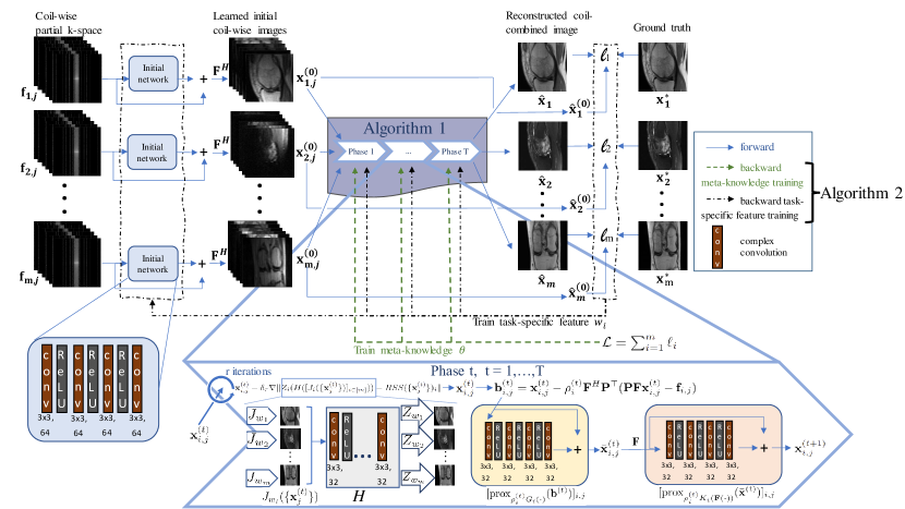
Figure 1: The proposed multi-task meta-learning MRI reconstruction.

2.1 Forward Learnable Optimization using Gradient Descent

We propose to develop an unrolled network to solve both the upper-level variational minimization problem and the lower-level constrained optimization problem in model (1). We introduce a proximal gradient descent [13] inspired algorithm 1, which can be parametrized as an iterative procedure with total $T$ iterations. The input $\mathbf{x}^{(0)}_{i,j}$ of the algorithm is obtained from an initial network that tries to pre-estimate the missing k-space data (similar to conventional parallel imaging methods such as GRAPPA [6]) therefore providing a good initial start for Algorithm 1. This helps reduce the number of iterations needed for convergence and decreases the overall computational complexity. The overall procedure consists of two for-loops: an outer and an inner loop, as follows:

1:  Input: $\mathbf{x}^{(0)}_{i,j},\delta_{0},\rho_{i}^{(0)}$.

2:  for $t=0,1,\dots,T-1$ do

3:     for $\tau=0,1,\dots,r$ do

4:        $\mathbf{x}^{(t)}_{i,j}\leftarrow{\mathbf{x}}^{(t)}_{i,j}-\delta_{\tau}\nabla\|Z_{i}(H([J_{i}(\{{\mathbf{x}}_{j}^{(t)}\})]_{i\in[m]}))-RSS(\{\mathbf{x}^{(t)}_{j}\})_{i}\|$

5:     end for

6:     $\mathbf{b}_{i,j}^{(t)}=\mathbf{x}_{i,j}^{(t)}-\rho^{(t)}_{i}\mathbf{F}^{H}\mathbf{P}^{\top}(\mathbf{P}\mathbf{F}\mathbf{x}_{i,j}^{(t)}-\mathbf{f}_{i,j}),\quad i=1,\cdots,m,\,j=1,\cdots,c,$

7:     $\bar{\mathbf{x}}_{i,j}^{(t)}=[\operatorname{\mathrm{prox}}_{\rho^{(t)}_{i}G_{i}(\cdot)}({\mathbf{b}}^{(t)})]_{i,j},\quad i=1,\cdots,m,\,j=1,\cdots,c,$

8:     ${\mathbf{x}}_{i,j}^{(t+1)}=[\operatorname{\mathrm{prox}}_{\rho^{(t)}_{i}K_{i}(\mathbf{F}(\cdot))}(\bar{\mathbf{x}}^{(t)})]_{i,j},\quad i=1,\cdots,m,\,j=1,\cdots,c,$

9:  end for and output $\mathbf{x}^{(T)}_{i,j}$, $Z_{i}(H([J_{i}(\{{\mathbf{x}}_{j}^{(T)}\})]_{i\in[m]}))$, $Z_{i}(H([J_{i}(\{{\mathbf{x}}_{j}^{(0)}\})]_{i\in[m]}))$

Algorithm 1 Forward Learnable Descent Algorithm for solving (1)

The inner loop aims to solve the lower-level optimization in (1b). We first calculate the gradient of the constrained least squares in (1b) and then iterate $r$ steps using gradient descent with a learnable step size $\delta_{\tau}$ shown in steps 3-5 in Algorithm 1. In the outer loop, the updated ${\mathbf{x}}^{(t)}_{i,j}$ serves as the initial input for steps 6-8 of proximal gradient descent. The proximal operator is defined as $\operatorname{\mathrm{prox}}_{\alpha R}(\mathbf{b}):=\operatorname*{arg\,min}_{\mathbf{x}}\left\{\frac{1}{2\alpha}\|\mathbf{x}-\mathbf{b}\|^{2}+R(\mathbf{x})\right\}$. In step 7 and 8, two proximal operators are conducted by alternating between image and k-space domains to ensure learning of both image and frequency features. Because the proximal operators do not have a closed-form solution for explicit implementation, we parametrize $\operatorname{\mathrm{prox}}_{\rho^{(t)}_{i}G_{i}(\cdot)}$ and $\operatorname{\mathrm{prox}}_{\rho^{(t)}_{i}K_{i}(\mathbf{F}(\cdot))}$ as two learnable deep residual networks in image and k-space domains, respectively, to emphasize artifacts and noise removal (in image domain) and structure preservation (in frequency domain). Our final outputs in step 9 from Algorithm 1 are reconstructed multi-coil images of all tasks $\mathbf{x}^{(T)}_{i,j}$, we then apply $Z_{i},H,J_{i}$ to obtain their corresponding coil-combined, meta-knowledge distributed image $\hat{\mathbf{x}}_{i}=Z_{i}(H([J_{i}(\{{\mathbf{x}}_{j}^{(T)}\})]_{i\in[m]}))$. In addition, we also apply $Z_{i},H,J_{i}$ to the initial reconstruction $\mathbf{x}^{(0)}_{i,j}$ and get $\hat{\mathbf{x}}_{i}^{(0)}=Z_{i}(H([J_{i}(\{{\mathbf{x}}_{j}^{(0)})\}]_{i\in[m]}))$. Both $\hat{\mathbf{x}}_{i}$ and $\hat{\mathbf{x}}_{i}^{(0)}$ are then input to the loss function. Our overall loss function is designed as follows for the forward optimization:

$$\textstyle{\mathcal{L}(\Theta,W;\mathcal{D}):=\sum^{m}_{i=1}\ell_{i}(\Theta,w_{i};\mathcal{D}_{i})},\text{ where each $\ell_{i}$ is called \emph{base-loss}:}$$ (2a)

$$\textstyle{\ell_{i}(\Theta,w_{i};\mathcal{D}_{i})=\|\hat{\mathbf{x}}_{i}(\Theta,w_{i})-\mathbf{x}^{*}_{i}\|+\lambda\|\hat{\mathbf{x}}_{i}^{(0)}(\Theta,w_{i})-\mathbf{x}^{*}_{i}\|-\mu\text{SSIM}(\hat{\mathbf{x}}_{i}(\Theta,w_{i}),\mathbf{x}^{*}_{i})},$$ (2b)

where we use $*$ to reflect the fully-sampled k-space and the ground truth for each task is $\mathbf{x}^{*}_{i}=RSS(\{\mathbf{x}^{*}_{j}\}_{j=1}^{c})_{i}$ and $\mathcal{D}_{i}={(\mathbf{f}_{i},\mathbf{x}^{*}_{i})}$ is the training data pair for the $i$-th task. The objective is to learn network weights $W$ and $\Theta$ during training. The loss function consists of three terms in (2). The first term is a standard supervised learning term forcing the final reconstructed image to approximate the target image from a fully-sampled k-space. The second term aims to learn a favorable initial input $\mathbf{x}^{(0)}_{i,j}$ for Algorithm 1. The third term uses the structural similarity index (SSIM) [17] to enforce the similarity between the reconstructed and target images. Parameters $\lambda$ and $\mu$ are prescribed to balance the three terms.

2.2 Backward Network Update through Meta-training

The backward operation (3) is conducted during training to minimize the overall loss function in (2) with respect to the network weights $\Theta$ and $W$.

$$\textstyle{\min_{\Theta(W)}\mathcal{L}(\Theta,W;\mathcal{D})}$$ (3a)

s.t. $$w_{i}=\textstyle{\operatorname*{arg\,min}_{w_{i}}\ell_{i}(\Theta(W),w_{i};\mathcal{D}_{i}),\quad i=1,\cdots,m}$$ (3b)

The overall procedure to solve (3) is inspired by Model-Agnostic Meta-Learning (MAML) [5] that consists of two for-loops: an outer and an inner loop, as follows:

11:  Input: $\mathcal{D}_{i}$ and initialize $\Theta$, ${w_{i}}$, $i=1,\cdots,m$.

2:  for $l=0,1,\dots,L$ do

3:     Sample training volume $\mathcal{V}_{i}\subset\mathcal{D}_{i}$.

4:     for $k=0,1,\dots,K$ (inner loop) do

5:        $\Theta\leftarrow\Theta-\beta\nabla_{\Theta}\mathcal{L}(\Theta,W;\{\mathcal{V}_{i}:i\in[m]\})$

6:     end for

7:     $w_{i}\leftarrow w_{i}-\alpha_{i}\nabla_{w_{i}}\ell_{i}(\Theta,w_{i};\mathcal{V}_{i}),\quad i=1,\cdots,m$

8:  end for and output $\Theta$, $W=\{w_{1},\cdots,w_{m}\}$

Algorithm 2 Backward Meta-Training algorithm for solving (3).

We train the outer loop with a total of $L$ epochs. A mini-batch training with a randomly selected 3D image volume is used in each epoch $l\in\{0,\cdots,L\}$. The inner loop aims to learn meta-knowledge $\Theta(W)$ through the upper-level (meta-level) minimization in (3a), where the meta-knowledge $\Theta$ is a function dependent on network weights $W$ (a.k.a., learning-to-learn). The upper-level minimization fixes $W$ and only updates $\Theta$ in the inner loop steps 4-6, and then the updated $\Theta(W)$ is used as input into lower-level (base-level) minimization to optimize each $w_{i}$ in (3b) in the outer loop. $\beta$ represents the meta-learning rate in the inner loop and $\alpha_{i}$ represents each base learning rate in the outer loop.

3 Experiments

3.1 Experiment Setup

The study was approved by the local IRB. Knee datasets with fully-sampled k-space were acquired on $25$ subjects (20/5 for training/testing). The datasets were acquired on a 3.0T scanner with an 18-element knee coil array using four two-dimensional fast spin-echo (FSE) sequences, including coronal proton density-weighted FSE (Cor-PD) and T2-weighted FSE (Cor-T2), and sagittal proton density-weighted FSE (Sag-PD) and T2-weighted FSE (Sag-T2).

Experiments were performed to evaluate the efficacy and efficiency of our proposed method to reconstruct highly-undersampled multi-task knee MRI. K-space data were retrospectively undersampled [10] to simulate acceleration rates (AR) of $\{4,5,6\}$. To illustrate the effect of meta-learning, we denote our proposed method without the meta-learner $H_{\Theta}$ (i.e., only iterate steps 6 to 8 in Algorithm 1 for m tasks separately) as single-task learning (STL) and the full version as multi-task meta-learning (MTML). All hyper-parameter selection is shown in the Appendix. We also compared our proposed STL and MTML against two recently developed reconstruction methods ISTA-Net [18] and pMRI-Net [2], both of which were previously shown to provide great performance in reconstructing undersampled single-task MRI data.

3.2 Experimental Results

Table 1: Quantitative comparison of different methods. (ITL: proposed single-task learning; MTML: proposed multi-task meta-learning; PSNR: peak signal-to-noise ratio; NMSE: normalized mean squared error)

		Sag-T2
AR	4x	5x	6x
	PSNR/SSIM/NMSE	PSNR/SSIM/NMSE	PSNR/SSIM/NMSE
ISTA-Net[18]	34.6138/0.9687/0.1444	33.4308/0.9600/0.1659	31.5700/0.9458/0.2061
pMRI-Net[2]	36.1084/0.9769/0.1214	35.0315/0.9712/0.1375	34.3608/0.9672/0.1486
ITL	37.4666/0.9825/0.1039	36.6242/0.9793/0.1144	35.9206/0.9763/0.1239
MTML	38.3446/0.9854/0.0941	37.5966/0.9832/0.1023	36.8210/0.9799/0.1118

		Cor-T2
	PSNR/SSIM/NMSE	PSNR/SSIM/NMSE	PSNR/SSIM/NMSE
ISTA-Net[18]	34.1552/0.9628/0.1142	32.7243/0.9472/0.1382	30.0678/0.9155/0.1864
pMRI-Net[2]	36.3567/0.9767/0.0867	35.5938/0.9728/0.0942	34.1399/0.9646/0.1108
ITL	37.0114/0.9796/0.0808	36.1727/0.9758/0.0883	35.7136/0.9739/0.0930
MTML	37.8478/0.9828/0.0740	37.1512/0.9812/0.0793	36.6107/0.9781/0.0843

		Sag-PD
	PSNR/SSIM/NMSE	PSNR/SSIM/NMSE	PSNR/SSIM/NMSE
ISTA-Net[18]	33.1395/0.9541/0.0774	31.9699/0.9495/0.0877	29.4236/0.9280/0.1176
pMRI-Net[2]	35.0189/0.9685/0.0623	34.1714/0.9588/0.0690	31.8230/0.9365/0.0906
ITL	35.9640/0.9736/0.0558	35.0720/0.9680/0.0617	34.0919/0.9619/0.0691
MTML	37.0246/0.9784/0.0493	36.2652/0.9754/0.0537	35.1452/0.9688/0.0611

		Cor-PD
	PSNR/SSIM/NMSE	PSNR/SSIM/NMSE	PSNR/SSIM/NMSE
ISTA-Net[18]	32.3933/0.9640/0.1030	31.1878/0.9555/0.1150	29.1795/0.9603/0.1281
pMRI-Net[2]	33.5534/0.9695/0.0937	32.7408/0.9667/0.1003	30.8576/0.9560/0.1178
ITL	35.5481/0.9760/0.0809	33.5579/0.9698/0.0939	31.9874/0.9625/0.1045
MTML	36.6621/0.9797/0.0748	35.4338/0.9765/0.0817	32.8284/0.9663/0.0999

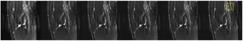
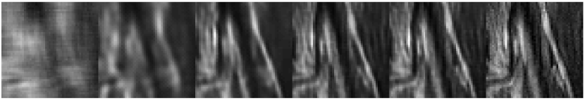
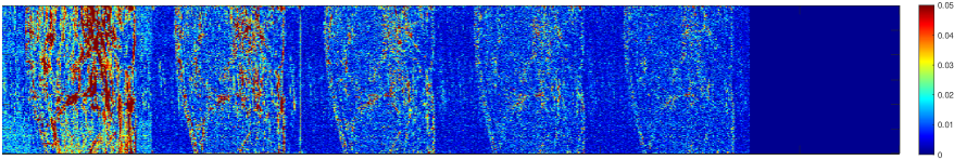
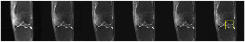
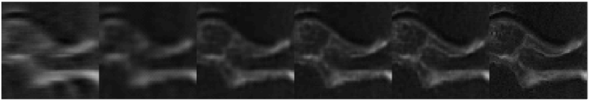
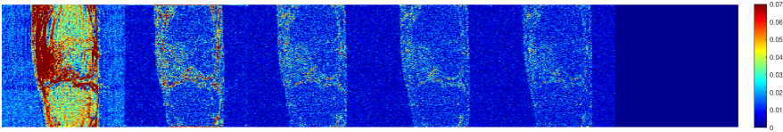
Figure 2: Comparison of Sag-T2 and Cor-T2 contrasts at AR = 6.

Fig. 2 compares the reconstructed images for Sag-T2 and Cor-T2 contrasts from different methods at AR=6. While ISTA-Net and pMRI-Net can largely remove the aliasing artifacts at this undersampling level, both methods yielded suboptimal reconstruction performance with noticeable image blurring in the reconstructed images. Our proposed STL can enable better reconstruction than ISTA-Net and pMRI-Net with improved image sharpness, due to its ability to cross-learn both image and k-space features, therefore better removing noises and artifacts and meanwhile preserving high-frequency image features. Our proposed MTML using meta-learning performs the best, outperforming all single-task learning methods. The pixel-wise error maps show that MTML has the smallest reconstruction errors compared to the fully-sampled reference, and the error is more homogeneous across the entire image domain for MTML. The zoom-in images further highlight the superb reconstruction performance of MTML where the tissue boundaries are better characterized at all tissue types (cartilage, meniscus, and muscle), and tissue texture, sharpness, and conspicuity are well-preserved. Similar comparisons of reconstructed images for the Sag-PD and Cor-PD sequences are shown in the Appendix, where MTML also consistently enables the best and most balanced performance on different types of contrast.

The qualitative comparison in Fig. 2 is further verified by different quantitative metrics shown in Table 1. The table shows the mean PSNR, SSIM, and NMSE for all tested subjects for all methods at three ARs=$\{4,5,6\}$. MTML achieves the best quantitative performance in all metrics at all ARs, consistent with the qualitative assessment in exemplified figures.

Our proof-of-concept study using multi-task meta-learning opens a new window for further investigating robust and efficient multi-contrast large-scale MRI reconstruction algorithms.

References

- [1] Antun, V., Renna, F., Poon, C., Adcock, B., Hansen, A.C.: On instabilities of deep learning in image reconstruction and the potential costs of ai. Proceedings of the National Academy of Sciences 117(48), 30088–30095 (2020)
- [2] Bian, W., Chen, Y., Ye, X.: Deep parallel mri reconstruction network without coil sensitivities. In: Machine Learning for Medical Image Reconstruction: Third International Workshop, MLMIR 2020, Held in Conjunction with MICCAI 2020, Lima, Peru, October 8, 2020, Proceedings 3. pp. 17–26. Springer (2020)
- [3] Bian, W., Chen, Y., Ye, X.: An optimal control framework for joint-channel parallel mri reconstruction without coil sensitivities. Magnetic Resonance Imaging (2022)
- [4] Džeroski, S., Ženko, B.: Is combining classifiers with stacking better than selecting the best one? Machine learning 54, 255–273 (2004)
- [5] Finn, C., Abbeel, P., Levine, S.: Model-agnostic meta-learning for fast adaptation of deep networks. In: International conference on machine learning. pp. 1126–1135. PMLR (2017)
- [6] Griswold, M.A., et al.: Generalized autocalibrating partially parallel acquisitions (grappa). Magnetic Resonance in Medicine: An Official Journal of the International Society for Magnetic Resonance in Medicine 47(6), 1202–1210 (2002)
- [7] Hospedales, T., Antoniou, A., Micaelli, P., Storkey, A.: Meta-learning in neural networks: A survey. IEEE transactions on pattern analysis and machine intelligence 44(9), 5149–5169 (2021)
- [8] Knoll, F., Hammernik, K., Zhang, C., Moeller, S., Pock, T., Sodickson, D.K., Akcakaya, M.: Deep-learning methods for parallel magnetic resonance imaging reconstruction: A survey of the current approaches, trends, and issues. IEEE signal processing magazine 37(1), 128–140 (2020)
- [9] Liu, F., Samsonov, A., Chen, L., Kijowski, R., Feng, L.: Santis: sampling-augmented neural network with incoherent structure for mr image reconstruction. Magnetic resonance in medicine 82(5), 1890–1904 (2019)
- [10] Lustig, M., Donoho, D., Pauly, J.M.: Sparse mri: The application of compressed sensing for rapid mr imaging. Magnetic Resonance in Medicine: An Official Journal of the International Society for Magnetic Resonance in Medicine 58(6), 1182–1195 (2007)
- [11] Lustig, M., Pauly, J.M.: Spirit: iterative self-consistent parallel imaging reconstruction from arbitrary k-space. Magnetic resonance in medicine 64(2), 457–471 (2010)
- [12] Otazo, R., Kim, D., Axel, L., Sodickson, D.K.: Combination of compressed sensing and parallel imaging for highly accelerated first-pass cardiac perfusion mri. Magnetic resonance in medicine 64(3), 767–776 (2010)
- [13] Parikh, N., Boyd, S.: Proximal algorithms. Foundations and Trends in optimization 1(3), 127–239 (2014)
- [14] Pruessmann, K.P., Weiger, M., Scheidegger, M.B., Boesiger, P.: Sense: sensitivity encoding for fast mri. Magnetic Resonance in Medicine: An Official Journal of the International Society for Magnetic Resonance in Medicine 42(5), 952–962 (1999)
- [15] Shimron, E., Tamir, J.I., Wang, K., Lustig, M.: Implicit data crimes: Machine learning bias arising from misuse of public data. Proceedings of the National Academy of Sciences 119(13), e2117203119 (2022)
- [16] Sodickson, D.K., Manning, W.J.: Simultaneous acquisition of spatial harmonics (smash): fast imaging with radiofrequency coil arrays. Magnetic resonance in medicine 38(4), 591–603 (1997)
- [17] Wang, Z., et al.: Image quality assessment: from error visibility to structural similarity. IEEE transactions on image processing 13(4), 600–612 (2004)
- [18] Zhang, J., Ghanem, B.: Ista-net: Interpretable optimization-inspired deep network for image compressive sensing. In: Proceedings of the IEEE conference on computer vision and pattern recognition. pp. 1828–1837 (2018)