Self-consistent single-nucleon potential at positive energy produced by semi-realistic interaction and its examination via nucleon-nucleus elastic scattering

Abstract

Based on the variational principle, self-consistent single-particle (s.p.) potentials at positive energies are discussed, which correspond to the real part of the optical potential as the single folding potential (SFP). The nuclear-matter s.p. potential produced by the semi-realistic nucleonic interaction M3Y-P6, which has links to the bare nucleonic interaction, resembles those extracted from the empirical optical potential. Applying M3Y-P6 both to the self-consistent mean-field calculations for the target nucleus and to the SFP for the scattered nucleon, we find that the differential cross-sections of the nucleon-nucleus elastic scattering are reproduced almost comparably to the empirical potentials up to $80\,\mathrm{MeV}$ incident energy. The results demonstrate that the s.p. potential compatible with available experimental data can be derived from a single energy-independent effective interaction in this wide energy range.

I Introduction

Many-body systems comprised of nucleons, from atomic nuclei to objects in the universe, are important ingredients of Nature. While primarily governed by the strong interaction, they often behave as quantum Fermi liquid [1], in which constituent nucleons move almost independently under a mean field (MF). At the ground state (g.s.), the nuclear MF contains correlation effects as incorporated by the Brueckner theory [2], and is nowadays discussed in terms of the Kohn-Sham (KS) method in the density functional theory [3]. In the KS method, properties of the whole many-fermion system can be described in terms of a collection of single-particle (s.p.) orbitals under the self-consistent MF (SCMF) constructed from effective interaction (or energy density functional) [4, 5].

Nuclear equation-of-state (EoS), i.e., the energy of the nuclear matter as a function of density and temperature ($T$) [6], plays a vital role in supernovae and neutron stars. Whereas the EoS at $T=0$ has been investigated relatively well in connection to the experimental data and the EoS at finite $T$ has often been developed by extending it [7, 8, 9], the finite-$T$ EoS has not sufficiently been verified by experiments. At finite $T$, the constituent nucleons distribute over a wide energy range. Therefore, it is desirable to handle the nucleonic states without discontinuity with respect to energy. The extension of the KS or the SCMF approaches to finite $T$ [10, 11], in which the energy of the system is described by the s.p. states obeying the Fermi-Dirac distribution function, is a promising tool to obtain the EoS in connection to experimental data. However, as the effective interactions have been examined only via the nuclear structure data, the reliability of these approaches has been limited to low $T\,(\lesssim\,10\mathrm{MeV}$) so far. In the supernovae, $T$ may reach as high as $T_{\mathrm{max}}\sim 30\,\mathrm{MeV}$ [12], at which nucleons distribute over s.p. energies $\epsilon$ up to a few times $T_{\mathrm{max}}$. Although some EoSs have been developed from the bare nucleonic interaction through sophisticated theoretical methods [13, 14] up to finite-$T$ cases [15, 16], they are not easily compared with a variety of experimental data. Since the energy distribution of nucleons is determined by the MF, i.e., the s.p. potential produced by the nucleonic interaction, it is a crucial step to examine whether the effective interaction produces adequate s.p. potential at $\epsilon>0$, as well as in the nuclear structure.

Nuclear MF at $\epsilon>0$ is connected to the nucleon-nucleus ($N$-$A$) elastic scattering. The $N$-$A$ elastic scattering is described by the optical potential $\mathcal{U}=\mathcal{V}+i\,\mathcal{W}$ [17, 18], where $\mathcal{V}$ and $\mathcal{W}$ are hermitian one-body operators, often expressed by real functions of the position. The imaginary part $\mathcal{W}$ carries effects of absorption, i.e., loss of the flux out of the elastic channel. Most conventionally, both $\mathcal{V}$ and $\mathcal{W}$ were adjusted to the data. A local function was assumed, with the parameters dependent on the incident energy and the mass number [19, 20]. The folding model has been developed to derive the optical potential from the nucleonic effective interaction [21], which does not need parameters depending on the mass number. There have been attempts to derive folding potentials from the bare nucleonic interaction [22, 23, 24, 25, 26, 27, 28].

Under the thermal equilibrium, there is no absorption because of the detailed balance between inflow and outflow. Only the real potential $\mathcal{V}$ is relevant, involving correlation effects like the s.p. potential in the KS theory. In this respect, $\mathcal{V}$ is of particular interest, which could be the s.p. potential at $\epsilon>0$ continuous with the MF potential in nuclear structure. The Skyrme and the Gogny interactions, which are effective interactions developed for nuclear SCMF calculations, have been applied to the $N$-$A$ elastic scattering [29, 30, 31, 32, 33, 34, 35, 36, 37]. However, the good applicability of these phenomenological interactions could be limited to low energy. Whereas the imaginary potential has also been argued within the many-body perturbation theory (MBPT) [30, 31, 34, 36, 38], correlation effects already contained in the effective interaction have yet to be subtracted. If we can develop a reliable real potential covering a wide energy range without counting on the MBPT, it could be a significant step toward a reasonable SCMF (or KS) approach at finite $T$. It should be mentioned that a Brueckner-Hartree-Fock approach to EoS combined with the $N$-$A$ scattering was reported in Ref. [39], though not precisely examined by nuclear structure.

The Michigan-three-range-Yukawa (M3Y) interaction was developed for $N$-$A$ inelastic scattering, based on the $G$-matrix [40, 41]. By introducing density-dependent coefficients, the M3Y interaction was extensively applied to the folding potential [42, 43]. One of the authors (H.N.) evolved M3Y-type effective interactions applicable to nuclear structure [44]. In particular, the parameter-set M3Y-P6 [45] has been scrutinized in the SCMF approach [46], and notable success has been found in describing the nuclear shell structure [46, 47], establishing reliability for s.p. potential at $\epsilon<0$. Moreover, M3Y-P6 is compatible with the EoS parameters at $T=0$ extracted by experiments and reproduces a microscopic neutron-matter EoS [45, 46]. It has also been pointed out that the M3Y-type interactions are almost free from unphysical instabilities in excitations of the nuclear matter [48], unlike many other MF interactions. A SCMF approach with M3Y-P6 has been extended to finite $T$ to investigate the liquid-gas phase transition occurring at $T\approx 10\,\mathrm{MeV}$ in Ref. [11]. It is interesting to examine this effective interaction for the $N$-$A$ scattering.

II Single folding potential and self-consistent mean field

Within the SCMF scheme, the total energy $E$ is represented by

$$E=\sum_{\alpha}\langle\alpha|\frac{\mathbf{p}^{2}}{2M}|\alpha\rangle\,n_{\alpha}+\frac{1}{2}\sum_{\alpha\beta}\langle\alpha\beta|\hat{v}|\alpha\beta\rangle\,n_{\alpha}\,n_{\beta}\,.$$ (1)

The indices $\alpha$ and $\beta$ denote s.p. states, which will be commonly used for labeling nucleons without confusion, $n_{\alpha}$ is the occupation probability on $\alpha$, and $\hat{v}$ is the two-body interaction, whose strengths may depend on the density. The s.p. Hamiltonian $h$ is derived as

$$h=\sum_{\alpha}\bigg{[}\Big{(}\frac{1}{n_{\alpha}}\,\frac{\delta E}{\delta\langle\alpha|}\Big{)}\bigg{|}_{n^{(0)}}\langle\alpha|\bigg{]}=\frac{\mathbf{p}^{2}}{2M}+U\,,$$ (2)

from which the s.p. state $|\alpha\rangle$ and its energy $\epsilon_{\alpha}$ are obtained via $h|\alpha\rangle=\epsilon_{\alpha}|\alpha\rangle$. We have defined $(\delta/\delta\langle\alpha|)\langle\alpha^{\prime}|\hat{\mathcal{O}}|\beta\rangle=\delta_{\alpha\alpha^{\prime}}\,\hat{\mathcal{O}}|\beta\rangle$ for a matrix element of a one-body operator $\hat{\mathcal{O}}$, and analogously for two-body matrix elements. The expression $|_{n^{(0)}}$ means substituting appropriate values $n_{\beta}^{(0)}$ for $n_{\beta}$. The second term on the right-hand side (rhs) of Eq. (1) leads to the s.p. potential $U$, which is non-local in general. For spherical nuclei, it is appropriate to take $\alpha=(\nu_{r}\ell jm\tau)$, where $\tau\,(=p,n)$ is the particle type, $(\ell jm)$ are the angular-momentum quantum numbers, and $\nu_{r}$ distinguishes radial wave-functions. For homogeneous nuclear matter, we take $\alpha=(\mathbf{k}\sigma\tau)$, with the momentum $\mathbf{k}$ and the $z$-component of the nucleon spin $\sigma$.

Suppose that $\hat{v}$ can be expressed as

$$\hat{v}=\sum_{i}C_{i}[\rho]\cdot\hat{w}_{i}\,,$$ (3)

where $\hat{w}_{i}$ is a two-body operator with strength $C_{i}$ that may depend on $\rho(\mathbf{r})$, as the interaction of Eq. (11) in Appendix A. Then, the s.p. potential $U$ in Eq. (2) becomes

$$\begin{split}U|\alpha\rangle=&\sum_{i}\sum_{\beta}\big{\langle}\!\!\ast\!\beta\big{|}C_{i}[\rho^{(0)}(\mathbf{R}_{\alpha\beta})]\cdot\hat{w}_{i}\big{|}\alpha\beta\big{\rangle}\,n_{\beta}^{(0)}\\ &+\frac{1}{2}\,|\alpha\rangle\,\sum_{i}\sum_{\alpha^{\prime}\beta}C^{\prime}_{i}[\rho^{(0)}(\mathbf{r}_{\alpha})]\,\big{\langle}\alpha^{\prime}\beta\big{|}\delta(\mathbf{r}_{\alpha}-\mathbf{R}_{\alpha^{\prime}\beta})\cdot\hat{w}_{i}\big{|}\alpha^{\prime}\beta\big{\rangle}\,n_{\alpha^{\prime}}^{(0)}\,n_{\beta}^{(0)}\,.\end{split}$$ (4)

We have assumed that $\rho$ depends on $\mathbf{R}_{\alpha\beta}:=(\mathbf{r}_{\alpha}+\mathbf{r}_{\beta})/2$ when it acts on two nucleons $\alpha$ and $\beta$. The expression $\langle\ast\beta|$ means that it is the result of the variation, $\langle\ast\beta|:=(\delta/\delta\langle\alpha|)\langle\alpha\beta|$, and $\rho^{(0)}$ is the density obtained by $n^{(0)}$. The second term on the rhs that includes $C^{\prime}_{i}=dC_{i}/d\rho$ is the rearrangement potential, for which we have inserted $\delta\rho(\mathbf{r})/\delta\langle\alpha|=\delta(\mathbf{r}_{\alpha}-\mathbf{r})\,|\alpha\rangle$.

In the homogeneous nuclear matter, Eq. (4) arrives at

$$\begin{split}&\langle\mathbf{k}\sigma\tau|U|\mathbf{k}\sigma\tau\rangle\\ &\quad=\sum_{i}C_{i}[\rho]\,\frac{\Omega}{(2\pi)^{3}}\sum_{\sigma^{\prime}\tau^{\prime}}\int_{k^{\prime}\leq k_{\mathrm{F}\tau^{\prime}}}d^{3}k^{\prime}\,\langle\mathbf{k}\sigma\tau\,\mathbf{k}^{\prime}\sigma^{\prime}\tau^{\prime}|\hat{w}_{i}|\mathbf{k}\sigma\tau\,\mathbf{k}^{\prime}\sigma^{\prime}\tau^{\prime}\rangle\\ &\qquad+\sum_{i}C^{\prime}_{i}[\rho]\,\frac{\Omega}{2(2\pi)^{6}}\sum_{\sigma\tau\sigma^{\prime}\tau^{\prime}}\int_{k\leq k_{\mathrm{F}\tau},k^{\prime}\leq k_{\mathrm{F}\tau^{\prime}}}d^{3}k\,d^{3}k^{\prime}\,\langle\mathbf{k}\sigma\tau\,\mathbf{k}^{\prime}\sigma^{\prime}\tau^{\prime}|\hat{w}_{i}|\mathbf{k}\sigma\tau\,\mathbf{k}^{\prime}\sigma^{\prime}\tau^{\prime}\rangle\,.\end{split}$$ (5)

Here $\Omega$ is the volume of the system, and $k_{\mathrm{F}\tau}$ $(\tau=p,n)$ denotes the Fermi momentum that is related to the density, $\rho_{\tau}=k_{\mathrm{F}\tau}^{3}/(3\pi^{2})$ and $\rho=\sum_{\tau}\rho_{\tau}$. Analytic formulae for the integration in Eq. (5) are given in Ref. [44]. The potential $\langle\mathbf{k}\sigma\tau|U|\mathbf{k}\sigma\tau\rangle$ depends on $\rho$ and the asymmetry parameter $\eta_{t}$, where $\eta_{t}:=\sum_{\tau}\tau\rho_{\tau}\big{/}\rho$ with $\tau=\pm 1$ in the summation, as well as on $k=|\mathbf{k}|$ and $\tau$.

Let us consider the $N$-$A$ elastic scattering, to which the above formulae are applicable. The incident nucleon is denoted by $N$ with the energy $\epsilon_{N}$ (the subscript $N$ will occasionally be replaced by $p$ or $n$ in Sec. IV), and the target nucleus by its mass number $A$, whose g.s. energy and density are expressed as $E_{A}$ and $\rho_{A}^{(0)}$. The occupation probabilities are $n_{N}^{(0)}=1$, $n_{\alpha}^{(0)}=1$ for $\alpha$ belonging to the occupied states of $A$, and $n_{\alpha}^{(0)}=0$ for all the other s.p. states. Whereas the increment of the density due to the scattered nucleon is infinitesimal at each position, its variation with respect to $\langle N|$ is not negligible [50]. Therefore, the s.p. potential of Eq. (4) for $N$ is given by

$$\begin{split}U|N\rangle=&\sum_{i}\sum_{\beta=1}^{A}\big{\langle}\!\!\ast\!\beta\big{|}C_{i}[\rho_{A}^{(0)}(\mathbf{R}_{N\beta})]\cdot\hat{w}_{i}\big{|}N\beta\big{\rangle}\,n_{\beta}^{(0)}\\ &+\frac{1}{2}\,|N\rangle\,\sum_{i}\sum_{\alpha,\beta=1}^{A}C^{\prime}_{i}[\rho_{A}^{(0)}(\mathbf{r}_{N})]\,\big{\langle}\alpha\beta\big{|}\delta(\mathbf{r}_{N}-\mathbf{R}_{\alpha\beta})\cdot\hat{w}_{i}\big{|}\alpha\beta\big{\rangle}\,n_{\alpha}^{(0)}\,n_{\beta}^{(0)}\,.\end{split}$$ (6)

This $U$ corresponds to the single folding potential (SFP), which generally has non-locality, owing to the exchange term. The incident energy is $\epsilon_{N}=E-E_{A}=\langle N|h|N\rangle/\langle N|N\rangle$. In addition to the first term on the rhs of Eq. (6), which is the conventional SFP, the rearrangement potential appears in the second term [49, 50, 51, 52]. When three-body interaction acts on the system, its effects are treated analogously. If correlation effects are embodied in the effective interaction as in the KS theory [5], the above $U$ can be identified with the real part of the optical potential $\mathcal{V}$. Relativistic effects may partly be incorporated into the effective interaction [23], as well. We denote $\mathcal{V}$ by $\mathcal{V}^{\mathrm{SFP}}$ when calculated via Eq. (6). The present derivation elucidates that the SFP is a self-consistent s.p. potential at positive energies, in complete analogy to the SCMF potential. It deserves noting that $U$ in Eq. (6) does not depend on $\epsilon_{N}$ when the non-locality is explicitly taken into account, as will be confirmed from the formulae in Appendix B.

III Single-particle potential in nuclear matter

In the homogeneous nuclear matter, $\epsilon_{N}=k^{2}/(2M)+\langle\mathbf{k}\sigma\tau|U|\mathbf{k}\sigma\tau\rangle$ with the potential of Eq. (5). The non-locality in $U$ can be absorbed in the momentum-dependence, which is further translated into the $\epsilon_{N}$-dependence without approximation, because the momentum $\mathbf{k}$ is a good quantum number. If the nuclear-matter energy is a quadratic function of $\eta_{t}$ to good approximation [53], the s.p. potential is represented as

$$\langle\mathbf{k}\sigma\tau|U|\mathbf{k}\sigma\tau\rangle\approx U_{0}(\epsilon_{N};\rho)+\tau\,U_{1}(\epsilon_{N};\rho)\,\eta_{t}\,,$$ (7)

corresponding to the Lane form [18]. The s.p. potential at the saturation density $\rho_{0}$ can be compared to the empirical local potential $\mathcal{V}^{\mathrm{emp}}$ at the center of heavy nuclei, ideally the $A\to\infty$ limit,

$$\lim_{A\to\infty}\mathcal{V}^{\mathrm{emp}}(\mathbf{r}=0)\approx U_{0}^{\mathrm{emp}}(\epsilon_{N};\rho_{0})-\tau\,U_{1}^{\mathrm{emp}}(\epsilon_{N};\rho_{0})\,\frac{N-Z}{A}\,.\quad\left(\tau=\left\{\begin{array}[]{ll}+1&\mbox{for $p$}\\ -1&\mbox{for $n$}\end{array}\right.\right)$$ (8)

In Fig. 1, $U_{0}$ and $U_{1}$ at $\rho=0.16\,\mathrm{fm}^{-3}$ are shown as a function of $\epsilon_{N}$. Several effective interactions that successfully describe nuclear structure are applied: Skyrme-SLy4 [54], Gogny-D1S [55] and M3Y-P6 [45]. $U_{0}^{\mathrm{emp}}$ and $U_{1}^{\mathrm{emp}}$ are displayed for comparison, for which we take those of Refs. [19] (CH89) and [20] (KD). The CH89 potential was fitted to the data in $10\leq\epsilon_{N}\leq 65\,\mathrm{MeV}$. The KD potential, applicable in $0.001\leq\epsilon_{N}\leq 200\,\mathrm{MeV}$, contains linear terms of $A$ to which small coefficients are attached. Though divergent at the $A\to\infty$ limit, these terms should correspond to expansion with respect to $A$. We plot $U_{0}^{\mathrm{emp}}$ and $U_{1}^{\mathrm{emp}}$ at $A=208$ and $400$ to view the values at large $A$.

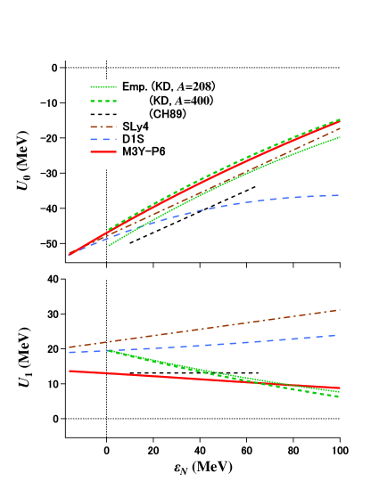
Figure 1: Energy dependence of $U_{0}$ and $U_{1}$ for homogeneous nuclear matter [see Eq. (7)] at $\rho=0.16\,\mathrm{fm}^{-3}$. The s.p. potentials given by the SCMF interactions, Skyrme-SLy4 (brown dot-dashed lines), Gogny-D1S (blue long-dashed lines) and M3Y-P6 (red solid lines), are compared with the empirical potentials, KD evaluated at $A=208$ (green dotted lines), at $A=400$ (green short-dashed lines) and CH89 (black short-dashed lines).

Although the empirical potentials do not match one another precisely, suggesting ambiguity in the extrapolation, the qualitative trend is similar. We point out that $U_{0}$ at the saturation energy $\epsilon_{N}\to\epsilon_{0}\approx-16\,\mathrm{MeV}$ is constrained by the condition $\epsilon_{0}=k_{\mathrm{F}}^{2}/(2M)+U_{0}(\epsilon_{0};\rho_{0})$. It is also noted that the slope of $U_{0}$ at $\epsilon_{0}$ corresponds to the effective mass (to be precise, the $k$-mass), which is constrained by the nuclear structure. Nevertheless, Fig. 1 clarifies that $U_{0}$ significantly depends on the effective interactions as $\epsilon_{N}$ becomes several tens MeV. In particular, the Gogny-D1S interaction provides $\epsilon_{N}$-dependence different from the empirical potentials. In contrast, $U_{0}$ with M3Y-P6 resembles $U_{0}^{\mathrm{emp}}$ of the KD potential for $A=400$. $U_{0}$ and $U_{1}$ with the Skyrme interaction are linear functions of $\epsilon_{N}$, and the $k$-mass determines the slope of $U_{0}$. $U_{0}$ from the Skyrme interaction does not severely deviate from the empirical potential as long as the $k$-mass has been adjusted as in SLy4, though it cannot describe a slight bend of $U_{0}$.

It is hard to constrain $U_{1}$ from the nuclear structure. The $\epsilon_{N}$-dependence of $U_{1}$ is distinctive among the effective interactions. M3Y-P6 provides $U_{1}$ almost consistent with the empirical potentials and with a microscopic result reported in Ref. [56], decreasing almost linearly for growing $\epsilon_{N}$, in contrast to SLy4 and D1S. These properties of M3Y-P6 could originate from its links to the bare nucleonic interaction. While the applications of the Skyrme and the Gogny interactions have been limited to $\epsilon_{N}\lesssim 30\,\mathrm{MeV}$, it will deserve testing M3Y-P6 for $N$-$A$ elastic scattering even at higher energies.

IV $N$-$A$ scattering cross-sections

We now turn to finite nuclei. As mentioned above, $U\,(=\mathcal{V}^{\mathrm{SFP}})$ of Eq. (6) provides a non-local potential, in general. Because the non-local SFP needs the s.p. wave-functions beyond the local density $\rho(\mathbf{r})$ and somewhat complicated computation, the local approximation has customarily been applied [57]. However, for consistency with the nuclear structure calculations, we apply the non-local SFP up to the non-central and Coulomb channels. Formulae deriving the non-local SFP from the effective interaction and the MF wave-functions are given in Appendix B. We emphasize that the present non-local SFP is independent of energy ($\epsilon_{N}$). The $\epsilon_{N}$-dependence of $U_{0}$ and $U_{1}$ in Fig. 1 results merely from converting the non-locality to the momentum dependence.

In this work, we investigate the $N$-$A$ elastic scattering at the incident energies ranging from $\epsilon_{N}\approx 10\,\mathrm{MeV}$ to $80\,\mathrm{MeV}$. For the target nuclei, we pick up ¹⁶O, ⁴⁰Ca, ⁹⁰Zr and ²⁰⁸Pb, which have $J^{\pi}=0^{+}$ and whose wave-function can reasonably be obtained by the spherical Hartree-Fock (HF) calculation. On top of the self-consistent HF wave-function of the target nucleus with M3Y-P6, the wave-function of the scattered nucleon is calculated under the optical potential, whose real part is taken from Eq. (6) with the same M3Y-P6 interaction. For the imaginary part, we employ the empirical potential $\mathcal{W}^{\mathrm{emp}}$ of Ref. [20], which is local and $\epsilon_{N}$-dependent. Thus, the optical potential is $\mathcal{U}=\mathcal{V}^{\mathrm{SFP}}+i\,\mathcal{W}^{\mathrm{emp}}$. We then compute physical quantities with the SIDES code [58]. Because the imaginary potential is connected to the inelastic scattering and the particle emission, its microscopic description should be consistent with these processes, and is left for future works. Whereas we have also tried other empirical imaginary potentials [19, 59, 60], the results are similar to those with the potential of Ref. [20]. Influence of the center-of-mass (c.m.) Hamiltonian on the $N$-$A$ scattering is discussed in Appendix. C. The $[-\mathbf{P}_{A}^{2}/(2AM)]$ term in Eq. (40) has been included in the HF calculations [46]. The c.m. correction of the first term on the rhs in Eq. (40) is handled within the SIDES code [58].

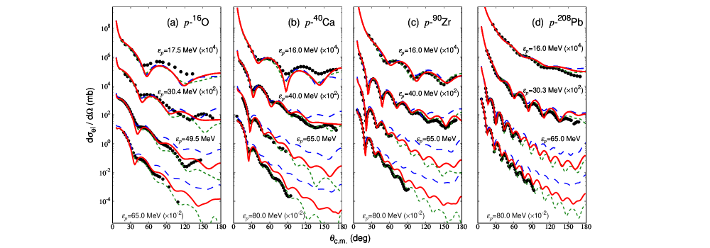
Figure 2: $d\sigma_{\mathrm{el}}/d\Omega$ of $p$-$A$ scattering: (a) $p$-¹⁶O, (b) $p$-⁴⁰Ca, (c) $p$-⁹⁰Zr and (d) $p$-²⁰⁸Pb. Results of $\mathcal{V}^{\mathrm{SFP}}$ with M3Y-P6 plus $\mathcal{W}^{\mathrm{emp}}$ are depicted by red solid lines and compared with experimental data (black circles) taken from the database [61], originally reported in Refs. [19, 62, 63, 64, 65, 66, 67, 68]. For comparison, results of $\mathcal{V}^{\mathrm{SFP}}$ with Gogny-D1S (blue long-dashed line), and those of $\mathcal{V}^{\mathrm{emp}}$ of Ref. [20] (green short-dashed lines) are also displayed. Depending on $\epsilon_{p}$, the cross sections are scaled by the coefficients in the parentheses.

In Fig. 2, the calculated differential cross-sections $d\sigma_{\mathrm{el}}/d\Omega$ of the proton-nucleus ($p$-$A$) scatterings are compared with the experimental data [61]. As well as the results of $\mathcal{V}^{\mathrm{SFP}}$ with M3Y-P6, we display the results with the Gogny-D1S interaction [55], and those applying the phenomenological potential of Ref.  [20] also to the real part, $\mathcal{V}^{\mathrm{emp}}$. Covering light to heavy nuclei ranging from $\epsilon_{p}\approx 15\,\mathrm{MeV}$ to $80\,\mathrm{MeV}$, the SFPs with M3Y-P6 reproduce $d\sigma_{\mathrm{el}}/d\Omega$ well, almost comparably to the empirical potential but without adjusting $\mathcal{V}$ to the scattering data. In particular, notable agreement with the data is found at $\epsilon_{p}=65\,\mathrm{MeV}$. At $\epsilon_{p}=80\,\mathrm{MeV}$, the calculated $d\sigma_{\mathrm{el}}/d\Omega$ is larger than the data at $\theta_{\mathrm{c.m.}}\gtrsim 60^{\circ}$. Still, the positions of the peaks and dips are well reproduced. In contrast, the D1S interaction gives $d\sigma_{\mathrm{el}}/d\Omega$ seriously deviating from the data in $\epsilon_{p}\gtrsim 65\mathrm{MeV}$, while it reproduces the cross sections at $\epsilon_{p}\lesssim 30\,\mathrm{MeV}$. This seems connected with the $\epsilon_{N}$-dependence of $U_{0}$ in Fig. 1.

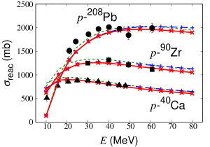
Figure 3: $\sigma_{\mathrm{reac}}$ of $p$-⁴⁰Ca, $p$-⁹⁰Zr and $p$-²⁰⁸Pb scattering. Results of $\mathcal{V}^{\mathrm{SFP}}$ with M3Y-P6 (D1S) plus $\mathcal{W}^{\mathrm{emp}}$ are plotted by crosses connected with red solid lines (pluses with blue long-dashed lines), and those of $\mathcal{V}^{\mathrm{emp}}$ are displayed by green short-dashed lines. Black circles, squares and triangles are experimental data [61, 69, 70, 71].

The optical theorem gives the total cross-section $\sigma_{\mathrm{tot}}$ [18], from which the reaction cross-section $\sigma_{\mathrm{reac}}$ is obtained as

$$\sigma_{\mathrm{reac}}=\sigma_{\mathrm{tot}}-\int d\Omega\,\frac{d\sigma_{\mathrm{el}}}{d\Omega}\,.$$ (9)

While both terms on the rhs are divergent in the $p$-$A$ scatterings, $\sigma_{\mathrm{reac}}$ is calculated in the SIDES code by properly treating the Coulombic contribution as discussed in Ref. [18]. Although $\sigma_{\mathrm{reac}}$ is primarily subject to the imaginary potential, the real potential indirectly influences $\sigma_{\mathrm{reac}}$. We show $\sigma_{\mathrm{reac}}$’s in the $p$-$A$ scatterings in Fig. 3 to examine the consistency of $\mathcal{W}^{\mathrm{emp}}$ combined with $\mathcal{V}^{\mathrm{SFP}}$. As expected, $\sigma_{\mathrm{reac}}$’s are insensitive to $\mathcal{V}$, and the application of $\mathcal{W}^{\mathrm{emp}}$ in combination with $\mathcal{V}^{\mathrm{SFP}}$ is justified in $10\lesssim\epsilon_{p}\lesssim 65\,\mathrm{MeV}$. Without available data, there remains room to improve $d\sigma_{\mathrm{el}}/d\Omega$ by readjusting $\mathcal{W}$ at $\epsilon_{p}\approx 80\,\mathrm{MeV}$, although an upper limit in $\epsilon_{N}$ is anticipated for the applicability of $\mathcal{V}^{\mathrm{SFP}}$, as argued below.

The calculated $d\sigma_{\mathrm{el}}/d\Omega$ of the neutron-nucleus ($n$-$A$) scatterings at $\epsilon_{n}\lesssim 30\,\mathrm{MeV}$ are compared with the experimental data [61] in Fig. 4. Data at higher energies are limited to small angles. It is confirmed that the calculated $\sigma_{\mathrm{tot}}$’s are compatible with the data in this energy range.

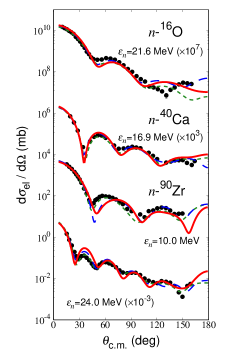
Figure 4: $d\sigma_{\mathrm{el}}/d\Omega$ of $n$-$A$ scattering: $n$-¹⁶O, $n$-⁴⁰Ca and $n$-⁹⁰Zr. Results of $\mathcal{V}^{\mathrm{SFP}}$ with M3Y-P6 and D1S, and those of $\mathcal{V}^{\mathrm{emp}}$ are presented, in comparison with experimental data  [61, 72, 73, 74]. See Fig. 2 for conventions.

Many effective interactions developed for scattering have explicit energy ($\epsilon$) dependence in their parameters, connected to the $\epsilon$-dependence of the $G$-matrix. However, the $\epsilon$-dependent interaction complicates treating the nuclear structure and finite-$T$ problems, in which a single system includes s.p. states with various energies. Therefore, $\epsilon$-independent effective interactions appropriately containing correlation effects are valuable. Still, it would be too optimistic to believe that we can remove $\epsilon$ dependence everywhere. There will be an upper limit of $\epsilon$ where the $\epsilon$-independent interaction works. It seems reasonable to consider that, for the present M3Y-P6 interaction, the upper limit lies around $\epsilon=80\,\mathrm{MeV}$.

In this paper, we have yet to discuss the analyzing power, on which some experimental data are available. The analyzing power is primarily relevant to the non-central channels, which do not contribute to the energy in homogeneous matter. We have confirmed that influence of the non-central channels, which are included except in the calculations for Fig. 1, is insignificant for $d\sigma_{\mathrm{el}}/d\Omega$. The analyzing power will be argued in a forthcoming paper [75].

V Summary and outlook

Based on the variational principle, we have discussed the self-consistent s.p. potential at positive energy. As it corresponds to the SFP and thereby to the real part of the optical potential, the property and validity of the potential can be examined via the $N$-$A$ elastic scattering.

For homogeneous nuclear matter, the non-locality of the potential is convertible to the $\epsilon$ dependence, where $\epsilon$ corresponds to the energy of the incident nucleon in the $N$-$A$ elastic scattering. We calculate the nuclear-matter s.p. potential with several effective interactions that work well for nuclear structure, and compare them to the empirical optical potentials at large $A$. It is found that some of them do not reproduce the $\epsilon$ dependence of the empirical potential. We have shown that the semi-realistic nucleonic interaction M3Y-P6, which has links to the bare nucleonic interaction, provides s.p. potentials similar to the empirical ones.

We have calculated the real part of the SFP fully consistent with the nuclear structure calculations. The differential cross-sections of the $N$-$A$ elastic scatterings have been computed by applying M3Y-P6 both to the SCMF calculations for the target nucleus and to the scattered nucleon’s SFP. The imaginary part of the optical potential, which carries the absorption effects, is complemented by the empirical one. It is confirmed that the SFP with M3Y-P6 describes the cross sections well, almost comparable to the empirical potentials, in as wide an energy range as $\epsilon\lesssim 80\,\mathrm{MeV}$. The reaction cross-sections of the proton scatterings and the total cross-sections of the neutron scatterings do not contradict the elastic scattering results.

United with the already established nuclear structure results, the present results demonstrate that s.p. potentials compatible with experimental data can be derived from a single $\epsilon$-independent effective interaction in a significantly extended energy range, indicating that the effective interaction properly takes account of many-body correlations. As the effective interaction is the only input in the SCMF (or KS) approach, these results may be a yardstick for extending the SCMF approach in nuclei to finite $T$ without artificial discontinuity with respect to energy.

Appendix A Effective Hamiltonian

In the subsequent Appendices, we consider the following Hamiltonian for the system comprised of $A^{\prime}$ nucleons,

$$\begin{split}H=&K+V_{N}+V_{C}-H_{\mathrm{c.m.}}\,;\\ &K=\sum_{\alpha}\frac{\mathbf{p}_{\alpha}^{2}}{2M}\,,\quad V_{N}=\sum_{\alpha<\beta}v_{\alpha\beta}\,,\quad V_{C}=\alpha_{\mathrm{em}}\sum_{\alpha<\beta(\in p)}\frac{1}{r_{\alpha\beta}}\,,\\ &H_{\mathrm{c.m.}}=\frac{\mathbf{P}^{2}}{2A^{\prime}M}=\frac{1}{A^{\prime}}\bigg{[}\sum_{\alpha}\frac{\mathbf{p}_{\alpha}^{2}}{2M}+\sum_{\alpha<\beta}\frac{\mathbf{p}_{\alpha}\cdot\mathbf{p}_{\beta}}{M}\bigg{]}\quad\Big{(}\mathbf{P}=\sum_{\alpha}\mathbf{p}_{\alpha}\Big{)}\,,\end{split}$$ (10)

where $\mathbf{r}_{\alpha\beta}=\mathbf{r}_{\alpha}-\mathbf{r}_{\beta}$ with $r=|\mathbf{r}|$, and $\alpha_{\mathrm{em}}$ (in $V_{C}$) is the fine structure constant. The effective nucleonic interaction $v_{\alpha\beta}$ is comprised of the following terms,

$$\begin{split}v_{\alpha\beta}=&v_{\alpha\beta}^{(\mathrm{C})}+v_{\alpha\beta}^{(\mathrm{LS})}+v_{\alpha\beta}^{(\mathrm{TN})}+v_{\alpha\beta}^{(\mathrm{C}\rho)}+v_{\alpha\beta}^{(\mathrm{LS}\rho)}\,;\\ &v_{\alpha\beta}^{(\mathrm{C})}=\sum_{k}\big{\{}t_{k}^{(\mathrm{SE})}P_{\mathrm{SE}}+t_{k}^{(\mathrm{TE})}P_{\mathrm{TE}}+t_{k}^{(\mathrm{SO})}P_{\mathrm{SO}}+t_{k}^{(\mathrm{TO})}P_{\mathrm{TO}}\big{\}}\,f_{k}^{(\mathrm{C})}(r_{\alpha\beta})\,,\\ &v_{\alpha\beta}^{(\mathrm{LS})}=\sum_{k}\big{\{}t_{k}^{(\mathrm{LSE})}P_{\mathrm{TE}}+t_{k}^{(\mathrm{LSO})}P_{\mathrm{TO}}\big{\}}\,f_{k}^{(\mathrm{LS})}(r_{\alpha\beta})\,\mathbf{L}_{\alpha\beta}\cdot(\mathbf{s}_{\alpha}+\mathbf{s}_{\beta})\,,\\ &v_{\alpha\beta}^{(\mathrm{TN})}=\sum_{k}\big{\{}t_{k}^{(\mathrm{TNE})}P_{\mathrm{TE}}+t_{k}^{(\mathrm{TNO})}P_{\mathrm{TO}}\big{\}}\,f_{k}^{(\mathrm{TN})}(r_{\alpha\beta})\,r_{\alpha\beta}^{2}S_{\alpha\beta}\,,\\ &v_{\alpha\beta}^{(\mathrm{C}\rho)}=\Big{\{}C_{\mathrm{SE}}[\rho(\mathbf{R}_{\alpha\beta})]\,P_{\mathrm{SE}}+C_{\mathrm{TE}}[\rho(\mathbf{R}_{\alpha\beta})]\,P_{\mathrm{TE}}\Big{\}}\,\delta(\mathbf{r}_{\alpha\beta})\,,\\ &v_{\alpha\beta}^{(\mathrm{LS}\rho)}=2i\,D[\rho(\mathbf{R}_{\alpha\beta})]\,\mathbf{p}_{\alpha\beta}\times\delta(\mathbf{r}_{\alpha\beta})\,\mathbf{p}_{\alpha\beta}\cdot(\mathbf{s}_{\alpha}+\mathbf{s}_{\beta})\\ &\qquad~{}=D[\rho(\mathbf{R}_{\alpha\beta})]\,\{-\nabla_{\alpha\beta}^{2}\,\delta(\mathbf{r}_{\alpha\beta})\}\,\mathbf{L}_{\alpha\beta}\cdot(\mathbf{s}_{\alpha}+\mathbf{s}_{\beta})\,,\end{split}$$ (11)

where $\mathbf{s}_{\alpha}$ is the spin operator, $\mathbf{R}_{\alpha\beta}=(\mathbf{r}_{\alpha}+\mathbf{r}_{\beta})/2$, $\mathbf{p}_{\alpha\beta}=(\mathbf{p}_{\alpha}-\mathbf{p}_{\beta})/2$, $\mathbf{L}_{\alpha\beta}=\mathbf{r}_{\alpha\beta}\times\mathbf{p}_{\alpha\beta}$, $S_{\alpha\beta}=4\,[3(\mathbf{s}_{\alpha}\cdot\hat{\mathbf{r}}_{\alpha\beta})(\mathbf{s}_{\beta}\cdot\hat{\mathbf{r}}_{\alpha\beta})-\mathbf{s}_{\alpha}\cdot\mathbf{s}_{\beta}]$, and $\rho(\mathbf{r})$ is the isoscalar nucleon density. $P_{\mathrm{Y}}$ ($\mathrm{Y}=\mathrm{SE},\mathrm{TE},\mathrm{SO},\mathrm{TO}$) stands for the projection operators on the singlet-even (SE), triplet-even (TE), singlet-odd (SO) and triplet-odd (TO) two-nucleon states. They are related to the spin- and isospin-exchange operators $P_{\sigma}\,[=(1+4\mathbf{s}_{\alpha}\cdot\mathbf{s}_{\beta})/2]$ and $P_{\tau}$ as

$$\begin{split}P_{\mathrm{SE}}=\frac{1-P_{\sigma}}{2}\,\frac{1+P_{\tau}}{2}\,,\quad&P_{\mathrm{TE}}=\frac{1+P_{\sigma}}{2}\,\frac{1-P_{\tau}}{2}\,,\\ P_{\mathrm{SO}}=\frac{1-P_{\sigma}}{2}\,\frac{1-P_{\tau}}{2}\,.\quad&P_{\mathrm{TO}}=\frac{1+P_{\sigma}}{2}\,\frac{1+P_{\tau}}{2}\,.\end{split}$$ (12)

Each channel $\mathrm{X}\,(=\mathrm{C},\mathrm{LS},\mathrm{TN}$) is composed of several terms distinguished by $k$, which corresponds to the function $f_{k}^{(\mathrm{X})}(r)$ and contains coupling constants $t_{k}^{(\mathrm{Y})}$. In the M3Y-type interaction, the Yukawa function $f_{k}^{(\mathrm{X})}(r)=e^{-x_{k}}/x_{k}$ with $x_{k}=\mu_{k}^{(\mathrm{X})}r$ is used for all of $\mathrm{X}=\mathrm{C},\mathrm{LS},\mathrm{TN}$, where $\mu_{k}^{-1}$ is the interaction range. In the conventional Gogny interaction, $f_{k}^{(\mathrm{C})}(r)=e^{-(\mu_{k}^{(\mathrm{C})}r)^{2}}$ and $f^{(\mathrm{LS})}(r)=\nabla^{2}\delta(\mathbf{r})$. The expression (11) also covers the Skyrme interaction by setting $f_{1}^{(\mathrm{C})}(r)=\delta(\mathbf{r})$, $f_{2}^{(\mathrm{C})}(r)=f^{(\mathrm{LS})}(r)=f^{(\mathrm{TN})}(r)=\nabla^{2}\delta(\mathbf{r})$ [76]. The $v^{(\mathrm{C}\rho)}$ and $v^{(\mathrm{LS}\rho)}$ terms have coupling constants $C_{\mathrm{Y}}[\rho]$ and $D[\rho]$ that depend on $\rho$, whose functional forms need not be specified here.

For later convenience, we rewrite $v_{\alpha\beta}^{(\mathrm{X})}$ ($\mathrm{X}=\mathrm{C},\mathrm{LS},\mathrm{TN}$) as

$$\begin{split}v_{\alpha\beta}^{(\mathrm{C})}=&\sum_{k}\Big{[}\big{\{}\bar{t}_{k}^{(0\mathrm{i})}+\bar{t}_{k}^{(0\mathrm{x})}P_{\tau}\big{\}}+(4\mathbf{s}_{\alpha}\cdot\mathbf{s}_{\beta})\,\big{\{}\bar{t}_{k}^{(1\mathrm{i})}\,+\bar{t}_{k}^{(1\mathrm{x})}\,P_{\tau}\big{\}}\Big{]}\,f_{k}^{(\mathrm{C})}(r_{\alpha\beta})\,;\\ &\qquad\bar{t}_{k}^{(0\mathrm{i})}=\frac{1}{8}\big{(}t_{k}^{(\mathrm{SE})}+3t_{k}^{(\mathrm{TE})}+t_{k}^{(\mathrm{SO})}+3t_{k}^{(\mathrm{TO})}\big{)}\,,\\ &\qquad\bar{t}_{k}^{(0\mathrm{x})}=\frac{1}{8}\big{(}t_{k}^{(\mathrm{SE})}-3t_{k}^{(\mathrm{TE})}-t_{k}^{(\mathrm{SO})}+3t_{k}^{(\mathrm{TO})}\big{)}\,,\\ &\qquad\bar{t}_{k}^{(1\mathrm{i})}=\frac{1}{8}\big{(}-t_{k}^{(\mathrm{SE})}+t_{k}^{(\mathrm{TE})}-t_{k}^{(\mathrm{SO})}+t_{k}^{(\mathrm{TO})}\big{)}\,,\\ &\qquad\bar{t}_{k}^{(1\mathrm{x})}=\frac{1}{8}\big{(}-t_{k}^{(\mathrm{SE})}-t_{k}^{(\mathrm{TE})}+t_{k}^{(\mathrm{SO})}+t_{k}^{(\mathrm{TO})}\big{)}\,,\\ v_{\alpha\beta}^{(\mathrm{LS})}=&\sum_{k}\big{\{}\bar{t}_{k}^{(\mathrm{LSi})}+\bar{t}_{k}^{(\mathrm{LSx})}P_{\tau}\big{\}}\,f_{k}^{(\mathrm{LS})}(r_{\alpha\beta})\,\mathbf{L}_{\alpha\beta}\cdot(\mathbf{s}_{\alpha}+\mathbf{s}_{\beta})\,;\\ &\qquad\bar{t}_{k}^{(\mathrm{LSi})}=\frac{1}{2}\big{(}t_{k}^{(\mathrm{LSE})}+t_{k}^{(\mathrm{LSO})}\big{)}\,,\quad\bar{t}_{k}^{(\mathrm{LSx})}=\frac{1}{2}\big{(}-t_{k}^{(\mathrm{LSE})}+t_{k}^{(\mathrm{LSO})}\big{)}\,,\\ v_{\alpha\beta}^{(\mathrm{TN})}=&\sum_{k}\big{\{}\bar{t}_{k}^{(\mathrm{TNi})}+\bar{t}_{k}^{(\mathrm{TNx})}P_{\tau}\big{\}}\,f_{k}^{(\mathrm{TN})}(r_{\alpha\beta})\,r_{\alpha\beta}^{2}S_{\alpha\beta}\,;\\ &\qquad\bar{t}_{k}^{(\mathrm{TNi})}=\frac{1}{2}\big{(}t_{k}^{(\mathrm{TNE})}+t_{k}^{(\mathrm{TNO})}\big{)}\,,\quad\bar{t}_{k}^{(\mathrm{TNx})}=\frac{1}{2}\big{(}-t_{k}^{(\mathrm{TNE})}+t_{k}^{(\mathrm{TNO})}\big{)}\,.\end{split}$$ (13)

The LS and tensor operators are expanded as, using $\bm{\ell}=\mathbf{r}\times\mathbf{p}$,

$$\begin{split}\mathbf{L}_{\alpha\beta}\cdot(\mathbf{s}_{\alpha}+\mathbf{s}_{\beta})&=\frac{1}{2}\big{\{}\bm{\ell}_{\alpha}\cdot\mathbf{s}_{\alpha}+\bm{\ell}_{\alpha}\cdot\mathbf{s}_{\beta}+\bm{\ell}_{\beta}\cdot\mathbf{s}_{\alpha}+\bm{\ell}_{\beta}\cdot\mathbf{s}_{\beta}+(\mathbf{r}_{\alpha}\times\mathbf{s}_{\alpha})\cdot\mathbf{p}_{\beta}-(\mathbf{p}_{\alpha}\times\mathbf{s}_{\alpha})\cdot\mathbf{r}_{\beta}\\ &\qquad\qquad-\mathbf{r}_{\alpha}\cdot(\mathbf{p}_{\beta}\times\mathbf{s}_{\beta})+\mathbf{p}_{\alpha}\cdot(\mathbf{r}_{\beta}\times\mathbf{s}_{\beta})\big{\}}\,,\\ r_{\alpha\beta}^{2}S_{\alpha\beta}=&16\pi\sum_{\lambda_{\alpha}\lambda_{\beta}}\delta_{\lambda_{\alpha}+\lambda_{\beta},2}\,\zeta_{\lambda_{\alpha}}\,r_{\alpha}^{\lambda_{\alpha}}r_{\beta}^{\lambda_{\beta}}\,\big{[}Y^{(\lambda_{\alpha})}(\hat{\mathbf{r}}_{\alpha})\,Y^{(\lambda_{\beta})}(\hat{\mathbf{r}}_{\beta})\big{]}^{(2)}\cdot[s_{\alpha}^{(1)}s_{\beta}^{(1)}]^{(2)}\,;\\ &\qquad\qquad\zeta_{0}=\zeta_{2}=\sqrt{\frac{6}{5}}\,,~{}\zeta_{1}=-2\,.\end{split}$$ (14)

Appendix B Formulae for single folding potential

This Appendix provides formulae to obtain the single folding potential (SFP) from the effective interaction in Appendix A. The wave function (w.f.) of the target nucleus is assumed to be obtained by a Hartree-Fock (HF) calculation.

In deriving the formulae of the SFP, we express the w.f. of the target nucleus via a set of the s.p. basis functions, which are denoted by $\varphi_{\alpha}(\mathbf{r}\sigma\tau)$, with the spin and isospin coordinates $\sigma$ and $\tau\,(=p,n)$. Instead of the occupation probability $n^{(0)}_{\alpha}$ in the text, we employ the one-body density matrix $\varrho_{\alpha\alpha^{\prime}}(:=\langle\Phi|a^{\dagger}_{\alpha^{\prime}}a_{\alpha}|\Phi\rangle)$. The w.f. of the projectile nucleon is represented by $\psi(\mathbf{r}\sigma\tau)$. The energy of the whole $N$-$A$ system is composed of the individual terms of the effective Hamiltonian. The SFP is expressed by a sum of the terms corresponding to those in Eq. (11),

$$\begin{split}U|N\rangle&=\sum_{\mathrm{X}}U^{(\mathrm{X})}|N\rangle\\ &=\sum_{\mathrm{X}}\bigg{\{}\sum_{\alpha\alpha^{\prime}\in A}\langle\ast\alpha^{\prime}|v^{\mathrm{(X)}}|N\alpha\rangle\,\varrho_{\alpha\alpha^{\prime}}+\frac{1}{2}\,|N\rangle\,\sum_{\alpha\alpha^{\prime}\beta\beta^{\prime}\in A}\big{\langle}\alpha^{\prime}\beta^{\prime}\big{|}\frac{\delta v^{\mathrm{(X)}}}{\delta\langle N|}\big{|}\alpha\beta\big{\rangle}\,\varrho_{\alpha\alpha^{\prime}}\,\varrho_{\beta\beta^{\prime}}\bigg{\}}\,.\end{split}$$ (15)

See the text for the notation. For density-independent channels ($\mathrm{X}=\mathrm{C},\mathrm{LS},\mathrm{TN}$), we have no rearrangement term, and Eq. (15) yields

$$\begin{split}U^{(\mathrm{X})}=&U^{(\mathrm{X,dir})}+U^{(\mathrm{X,exc})}\,;\\ &\quad\big{[}U^{(\mathrm{X,dir})}\psi\big{]}(\mathbf{r}\sigma\tau)=\sum_{\alpha\alpha^{\prime}\in A}\varrho_{\alpha\alpha^{\prime}}\sum_{\sigma^{\prime}\tau^{\prime}}\int d^{3}r^{\prime}\,\varphi_{\alpha^{\prime}}^{\ast}(\mathbf{r}^{\prime}\sigma^{\prime}\tau^{\prime})\,v^{(\mathrm{X})}\,\varphi_{\alpha}(\mathbf{r}^{\prime}\sigma^{\prime}\tau^{\prime})\,\psi(\mathbf{r}\sigma\tau)\,,\\ &\quad\big{[}U^{(\mathrm{X,exc})}\psi\big{]}(\mathbf{r}\sigma\tau)=-\sum_{\alpha\alpha^{\prime}\in A}\varrho_{\alpha\alpha^{\prime}}\sum_{\sigma^{\prime}\tau^{\prime}}\int d^{3}r^{\prime}\,\varphi_{\alpha^{\prime}}^{\ast}(\mathbf{r}^{\prime}\sigma^{\prime}\tau^{\prime})\,v^{(\mathrm{X})}\,\varphi_{\alpha}(\mathbf{r}\sigma\tau)\,\psi(\mathbf{r}^{\prime}\sigma^{\prime}\tau^{\prime})\,.\end{split}$$ (16)

The Coulomb interaction can be handled analogously. The density-dependent channels of Eq. (15) ($\mathrm{X}=\mathrm{C}\rho,\mathrm{LS}\rho$) will be discussed without separating the direct and exchange terms since they are assumed to be zero range, though the density-dependence leads to the rearrangement term (the second term on the rhs).

In the following, we omit the subscript $N$ for the projectile unless it leads to confusion. Furthermore, we drop the subscript $k$ that distinguishes the range parameters in Eq. (11), and the summation over $k$, though each channel may include plural terms having different ranges. Spherical basis functions are adopted for $\varphi_{\alpha}$ and the partial-wave expansion is applied to $\psi$,

$$\begin{split}\varphi_{\alpha}(\mathbf{r}\sigma\tau)&=\delta_{\tau\tau_{\alpha}}R_{\nu_{\alpha}\ell_{\alpha}j_{\alpha}}(r)\,[Y^{(\ell_{\alpha})}(\hat{\mathbf{r}})\,\chi_{\sigma}^{(1/2)}]^{(j_{\alpha})}_{m_{\alpha}}\,\xi_{\tau}\,,\\ \psi(\mathbf{r}\sigma\tau_{N})&=\delta_{\tau\tau_{N}}\sum_{\ell jm}c_{\ell jm}\mathcal{R}_{\ell j}(r)\,[Y^{(\ell)}(\hat{\mathbf{r}})\,\chi_{\sigma}^{(1/2)}]^{(j)}_{m}\,\xi_{\tau}\,,\end{split}$$ (17)

where $\chi_{\sigma}$ ($\xi_{\tau}$) is the spin (isospin) w.f. and $c_{\ell jm}$ is an appropriate coefficient. If the target has $J^{\pi}=0^{+}$, the density matrix has the property $\varrho_{\alpha\alpha^{\prime}}=\delta_{\tau_{\alpha}\tau_{\alpha^{\prime}}}\delta_{\ell_{\alpha}\ell_{\alpha^{\prime}}}\delta_{j_{\alpha}j_{\alpha^{\prime}}}\delta_{m_{\alpha}m_{\alpha^{\prime}}}\,\varrho^{(\tau_{\alpha}\ell_{\alpha}j_{\alpha})}_{\nu_{\alpha}\nu_{\alpha^{\prime}}}$. The quantum numbers $(\ell jm)$ do not mix in $\psi$, with $c_{\ell jm}$ fixed by the incident wave. The SFP is obtained for each $(\ell j)$, which will be denoted by $U_{\ell j}^{(\mathrm{X})}$.

The function $f(r_{\alpha\beta})$ in Eq. (11) is expanded as

$$f(r_{\alpha\beta})=\sum_{\lambda}g_{\lambda}(r_{\alpha},r_{\beta})\,P_{\lambda}(\hat{\mathbf{r}}_{\alpha}\cdot\hat{\mathbf{r}}_{\beta})=\sum_{\lambda}\frac{4\pi}{2\lambda+1}\,g_{\lambda}(r_{\alpha},r_{\beta})\,Y^{(\lambda)}(\hat{\mathbf{r}}_{\alpha})\cdot Y^{(\lambda)}(\hat{\mathbf{r}}_{\beta})\,,$$ (18)

where $P_{\lambda}$ is the Legendre polynomial and

$$g_{\lambda}(r_{\alpha},r_{\beta})=\frac{2\lambda+1}{2}\,\int_{-1}^{1}d(\cos\theta)\,f\Big{(}\sqrt{r_{\alpha}^{2}+r_{\beta}^{2}-2r_{\alpha}r_{\beta}\cos\theta}\,\Big{)}\,P_{\lambda}(\cos\theta)\,.$$ (19)

The form of $g_{\lambda}$ for several functions will be given later.

B.1 Terms from central channels

The contribution of $v^{(\mathrm{C})}$ to the SFP for each $(\ell,j)$ partial wave is represented as

$$\begin{split}U^{(\mathrm{C,dir})}_{\ell j}&=\sum_{\gamma=0,1}\sum_{\tau_{\alpha}}\big{\{}\bar{t}^{(\gamma\mathrm{i})}+\delta_{\tau\tau_{\alpha}}\bar{t}^{(\gamma\mathrm{x})}\big{\}}\,F^{(\mathrm{dir},\gamma)}_{\ell j,\tau_{\alpha}}\,;\\ &\quad F^{(\mathrm{dir},\gamma)}_{\ell j,\tau_{\alpha}}=\sum_{\begin{subarray}{c}\ell_{\alpha}j_{\alpha}m_{\alpha}\\ \nu_{\alpha}\nu_{\alpha^{\prime}}(\in A)\end{subarray}}\varrho^{(\tau_{\alpha}\ell_{\alpha}j_{\alpha})}_{\nu_{\alpha}\nu_{\alpha^{\prime}}}\sum_{\sigma^{\prime}\tau^{\prime}}\int d^{3}r^{\prime}\,\big{\{}R_{\nu_{\alpha^{\prime}}\ell_{\alpha}j_{\alpha}}(r^{\prime})\,[Y^{(\ell_{\alpha})}(\hat{\mathbf{r}}^{\prime})\,\chi_{\sigma^{\prime}}^{(1/2)}]^{(j_{\alpha})}_{m_{\alpha}}\big{\}}^{\ast}\\ &\hskip 142.26378pt\times f^{(\mathrm{C})}\big{(}|\mathbf{r}-\mathbf{r}^{\prime}|\big{)}\,\mathcal{O}^{(\mathrm{C},\gamma)}_{\sigma}\,\big{\{}R_{\nu_{\alpha}\ell_{\alpha}j_{\alpha}}(r^{\prime})\,[Y^{(\ell_{\alpha})}(\hat{\mathbf{r}}^{\prime})\,\chi_{\sigma^{\prime}}^{(1/2)}]^{(j_{\alpha})}_{m_{\alpha}}\big{\}}\,,\\ U^{(\mathrm{C,exc})}_{\ell j}&=-\sum_{\gamma=0,1}\sum_{\tau_{\alpha}}\big{\{}\bar{t}^{(\gamma\mathrm{x})}+\delta_{\tau\tau_{\alpha}}\bar{t}^{(\gamma\mathrm{i})}\big{\}}\,F^{(\mathrm{exc},\gamma)}_{\ell j,\tau_{\alpha}}\,;\\ &\quad F^{(\mathrm{exc},\gamma)}_{\ell j,\tau_{\alpha}}\,\big{\{}\mathcal{R}_{\ell j}(r)\,[Y^{(\ell)}(\hat{\mathbf{r}})\,\chi_{\sigma}^{(1/2)}]^{(j)}_{m}\big{\}}\\ &\qquad=\sum_{\begin{subarray}{c}\ell_{\alpha}j_{\alpha}m_{\alpha}\\ \nu_{\alpha}\nu_{\alpha^{\prime}}(\in A)\end{subarray}}\varrho^{(\tau_{\alpha}\ell_{\alpha}j_{\alpha})}_{\nu_{\alpha}\nu_{\alpha^{\prime}}}\sum_{\sigma^{\prime}\tau^{\prime}}\int d^{3}r^{\prime}\,\big{\{}R_{\nu_{\alpha^{\prime}}\ell_{\alpha}j_{\alpha}}(r^{\prime})\,[Y^{(\ell_{\alpha})}(\hat{\mathbf{r}}^{\prime})\,\chi_{\sigma^{\prime}}^{(1/2)}]^{(j_{\alpha})}_{m_{\alpha}}\big{\}}^{\ast}\,f^{(\mathrm{C})}\big{(}|\mathbf{r}-\mathbf{r}^{\prime}|\big{)}\,\mathcal{O}^{(\mathrm{C},\gamma)}_{\sigma}\\ &\hskip 142.26378pt\times\big{\{}R_{\nu_{\alpha}\ell_{\alpha}j_{\alpha}}(r)\,[Y^{(\ell_{\alpha})}(\hat{\mathbf{r}})\,\chi_{\sigma}^{(1/2)}]^{(j_{\alpha})}_{m_{\alpha}}\big{\}}\,\big{\{}\mathcal{R}_{\ell j}(r^{\prime})\,[Y^{(\ell)}(\hat{\mathbf{r}}^{\prime})\,\chi_{\sigma^{\prime}}^{(1/2)}]^{(j)}_{m}\big{\}}\,,\\ &\hskip 227.62204pt(\mathcal{O}^{(\mathrm{C},0)}_{\sigma}=1\,,~{}\mathcal{O}^{(\mathrm{C},1)}_{\sigma}=4\mathbf{s}\cdot\mathbf{s}^{\prime})\,.\end{split}$$ (20)

While $F^{(\mathrm{dir},\gamma)}_{\ell j,\tau_{\alpha}}$ provides a local potential, $F^{(\mathrm{exc},\gamma)}_{\ell j,\tau_{\alpha}}$ is an integral operator whose kernel corresponds to a non-local SFP. It acts on $\mathcal{R}_{\ell j}$ without influencing the angular-spin function. The effect of $F^{(\mathrm{exc},\gamma)}_{\ell j,\tau_{\alpha}}$ becomes transparent by integrating out the angular-spin part,

$$F^{(\mathrm{exc},\gamma)}_{\ell j,\tau_{\alpha}}\,\mathcal{R}_{\ell j}(r)=\sum_{\sigma}\int d\Omega\,\big{\{}[Y^{(\ell)}(\hat{\mathbf{r}})\,\chi_{\sigma}^{(1/2)}]^{(j)}_{m}\big{\}}^{\ast}\,F^{(\mathrm{exc},\gamma)}_{\ell j,\tau_{\alpha}}\,\big{\{}\mathcal{R}_{\ell j}(r)\,[Y^{(\ell)}(\hat{\mathbf{r}})\,\chi_{\sigma}^{(1/2)}]^{(j)}_{m}\big{\}}\,,$$ (21)

where $\int d\Omega$ is the integration over the solid angle. The Racah algebra to the angular-spin part yields

$$\begin{split}F^{(\mathrm{dir},\gamma)}_{\ell j,\tau_{\alpha}}=&\,\delta_{\gamma 0}\sum_{\begin{subarray}{c}\ell_{\alpha}j_{\alpha}\\ \nu_{\alpha}\nu_{\alpha^{\prime}}(\in A)\end{subarray}}(2j_{\alpha}+1)\,\varrho^{(\tau_{\alpha}\ell_{\alpha}j_{\alpha})}_{\nu_{\alpha}\nu_{\alpha^{\prime}}}\int r^{\prime\,2}dr^{\prime}\,g_{0}(r,r^{\prime})\,R_{\nu_{\alpha^{\prime}}\ell_{\alpha}j_{\alpha}}^{\ast}(r^{\prime})\,R_{\nu_{\alpha}\ell_{\alpha}j_{\alpha}}(r^{\prime})\,,\\ F^{(\mathrm{exc},\gamma)}_{\ell j,\tau_{\alpha}}\,\mathcal{R}_{\ell j}(r)=&\,2\,(2\gamma+1)\,\sum_{\begin{subarray}{c}\ell_{\alpha}j_{\alpha}\\ \nu_{\alpha}\nu_{\alpha^{\prime}}(\in A)\end{subarray}}(2\ell_{\alpha}+1)\,(2j_{\alpha}+1)\,\varrho^{(\tau_{\alpha}\ell_{\alpha}j_{\alpha})}_{\nu_{\alpha}\nu_{\alpha^{\prime}}}\\ &\hskip 56.9055pt\times\sum_{\lambda\kappa}(2\kappa+1)\,\big{(}\ell_{\alpha}\,0\,\lambda\,0\,|\,\ell\,0\big{)}^{2}\begin{Bmatrix}\ell_{\alpha}&1/2&j_{\alpha}\\ \lambda&\gamma&\kappa\\ \ell&1/2&j\end{Bmatrix}^{2}\\ &\hskip 113.81102pt\times\int r^{\prime\,2}dr^{\prime}\,g_{\lambda}(r,r^{\prime})\,R_{\nu_{\alpha^{\prime}}\ell_{\alpha}j_{\alpha}}^{\ast}(r^{\prime})\,R_{\nu_{\alpha}l_{\alpha}j_{\alpha}}(r)\,\mathcal{R}_{\ell j}(r^{\prime})\,.\end{split}$$ (22)

B.2 Terms from tensor channels

The contribution of $v^{(\mathrm{TN})}$ to the SFP is

$$\begin{split}U^{(\mathrm{TN,dir})}_{\ell j}&=0\,,\\ U^{(\mathrm{TN,exc})}_{\ell j}&=-\sum_{\tau_{\alpha}}\big{\{}\bar{t}^{(\mathrm{TNx})}+\delta_{\tau\tau_{\alpha}}\bar{t}^{(\mathrm{TNi})}\big{\}}\,F^{(\mathrm{exc,TN})}_{\ell j,\tau_{\alpha}}\,;\\ &\quad F^{(\mathrm{exc,TN})}_{\ell j,\tau_{\alpha}}\,\big{\{}\mathcal{R}_{\ell j}(r)\,[Y^{(\ell)}(\hat{\mathbf{r}})\,\chi_{\sigma}^{(1/2)}]^{(j)}_{m}\big{\}}\\ &\qquad=\sum_{\begin{subarray}{c}\ell_{\alpha}j_{\alpha}m_{\alpha}\\ \nu_{\alpha}\nu_{\alpha^{\prime}}(\in A)\end{subarray}}\varrho^{(\tau_{\alpha}\ell_{\alpha}j_{\alpha})}_{\nu_{\alpha}\nu_{\alpha^{\prime}}}\sum_{\sigma^{\prime}\tau^{\prime}}\int d^{3}r^{\prime}\,\big{\{}R_{\nu_{\alpha^{\prime}}\ell_{\alpha}j_{\alpha}}(r^{\prime})\,[Y^{(\ell_{\alpha})}(\hat{\mathbf{r}}^{\prime})\,\chi_{\sigma^{\prime}}^{(1/2)}]^{(j_{\alpha})}_{m_{\alpha}}\big{\}}^{\ast}\,f^{(\mathrm{TN})}\big{(}|\mathbf{r}-\mathbf{r}^{\prime}|\big{)}\\ &\hskip 42.67912pt\times\Big{\{}16\pi\sum_{\lambda_{1}\lambda_{2}}\delta_{\lambda_{1}+\lambda_{2},2}\,\zeta_{\lambda_{1}}\,r^{\lambda_{1}}r^{\prime,\lambda_{2}}\,\big{[}Y^{(\lambda_{1})}(\hat{\mathbf{r}})\,Y^{(\lambda_{2})}(\hat{\mathbf{r}}^{\prime})\big{]}^{(2)}\cdot[s^{(1)}s^{\prime(1)}]^{(2)}\Big{\}}\\ &\hskip 56.9055pt\times\big{\{}R_{\nu_{\alpha}\ell_{\alpha}j_{\alpha}}(r)\,[Y^{(\ell_{\alpha})}(\hat{\mathbf{r}})\,\chi_{\sigma}^{(1/2)}]^{(j_{\alpha})}_{m_{\alpha}}\big{\}}\,\big{\{}\mathcal{R}_{\ell j}(r^{\prime})\,[Y^{(\ell)}(\hat{\mathbf{r}}^{\prime})\,\chi_{\sigma^{\prime}}^{(1/2)}]^{(j)}_{m}\big{\}}\,.\\ \end{split}$$ (23)

The direct term vanishes because of the time-reversal symmetry in the target w.f. After dropping the angular-spin part, an algebra similar to Eq. (21) derives

$$\begin{split}&F^{(\mathrm{exc,TN})}_{\ell j,\tau_{\alpha}}\,\mathcal{R}_{\ell j}(r)\\ &\quad=\,30\sum_{\lambda_{1}\lambda_{2}}\delta_{\lambda_{1}+\lambda_{2},2}\,(-)^{\lambda_{1}+1}\,\zeta_{\lambda_{1}}\,\sqrt{(2\lambda_{1}+1)\,(2\lambda_{2}+1)}\sum_{\begin{subarray}{c}\ell_{\alpha}j_{\alpha}\\ \nu_{\alpha}\nu_{\alpha^{\prime}}(\in A)\end{subarray}}(2\ell_{\alpha}+1)\,(2j_{\alpha}+1)\,\varrho^{(\tau_{\alpha}\ell_{\alpha}j_{\alpha})}_{\nu_{\alpha}\nu_{\alpha^{\prime}}}\\ &\hskip 28.45274pt\times\sum_{\lambda\kappa\kappa_{1}\kappa_{2}}(2\kappa+1)\sqrt{(2\kappa_{1}+1)\,(2\kappa_{2}+1)}\,\big{(}\lambda\,0\,\lambda_{1}\,0\,|\,\kappa_{1}\,0\big{)}\,\big{(}\lambda\,0\,\lambda_{2}\,0\,|\,\kappa_{2}\,0\big{)}\\ &\hskip 56.9055pt\times\big{(}\ell_{\alpha}\,0\,\kappa_{1}\,0\,|\,\ell\,0\big{)}\,\big{(}\ell_{\alpha}\,0\,\kappa_{2}\,0\,|\,\ell\,0\big{)}\,W(2\,\lambda_{2}\,\kappa_{1}\,\lambda\,;\,\lambda_{1}\,\kappa_{2})\,W(2\,1\,\kappa_{1}\,\kappa\,;\,1\,\kappa_{2})\\ &\hskip 227.62204pt\times\begin{Bmatrix}\ell_{\alpha}&1/2&j_{\alpha}\\ \kappa_{1}&1&\kappa\\ \ell&1/2&j\end{Bmatrix}\,\begin{Bmatrix}\ell_{\alpha}&1/2&j_{\alpha}\\ \kappa_{2}&1&\kappa\\ \ell&1/2&j\end{Bmatrix}\\ &\hskip 142.26378pt\times\int r^{\prime\,2}dr^{\prime}\,r^{\lambda_{1}}r^{\prime\,\lambda_{2}}\,g_{\lambda}(r,r^{\prime})\,R_{\nu_{\alpha^{\prime}}\ell_{\alpha}j_{\alpha}}^{\ast}(r^{\prime})\,R_{\nu_{\alpha}\ell_{\alpha}j_{\alpha}}(r)\,\mathcal{R}_{\ell j}(r^{\prime})\,.\\ \end{split}$$ (24)

B.3 Terms from LS channels

The contribution of $v^{(\mathrm{LS})}$ to the SFP is, after taking into account the time-reversality for the direct term,

$$\begin{split}U^{(\mathrm{LS,dir})}_{\ell j}&=\sum_{\tau_{\alpha}}\big{\{}\bar{t}^{(\mathrm{LSi})}+\delta_{\tau\tau_{\alpha}}\bar{t}^{(\mathrm{LSx})}\big{\}}\,F^{(\mathrm{dir,LS})}_{\ell j,\tau_{\alpha}}\,;\\ &\quad F^{(\mathrm{dir,LS})}_{\ell j,\tau_{\alpha}}\,\big{\{}\mathcal{R}_{\ell j}(r)\,[Y^{(\ell)}(\hat{\mathbf{r}})\,\chi_{\sigma}^{(1/2)}]^{(j)}_{m}\big{\}}\\ &\qquad=\sum_{\begin{subarray}{c}\ell_{\alpha}j_{\alpha}m_{\alpha}\\ \nu_{\alpha}\nu_{\alpha^{\prime}}(\in A)\end{subarray}}\varrho^{(\tau_{\alpha}\ell_{\alpha}j_{\alpha})}_{\nu_{\alpha}\nu_{\alpha^{\prime}}}\sum_{\sigma^{\prime}\tau^{\prime}}\int d^{3}r^{\prime}\,\big{\{}R_{\nu_{\alpha^{\prime}}\ell_{\alpha}j_{\alpha}}(r^{\prime})\,[Y^{(\ell_{\alpha})}(\hat{\mathbf{r}}^{\prime})\,\chi_{\sigma^{\prime}}^{(1/2)}]^{(j_{\alpha})}_{m_{\alpha}}\big{\}}^{\ast}\\ &\hskip 42.67912pt\times f^{(\mathrm{LS})}\big{(}|\mathbf{r}-\mathbf{r}^{\prime}|\big{)}\,\Big{[}\frac{1}{2}\big{\{}\bm{\ell}\cdot\mathbf{s}+\bm{\ell}^{\prime}\cdot\mathbf{s}^{\prime}-(\mathbf{p}\times\mathbf{s})\cdot\mathbf{r}^{\prime}-\mathbf{r}\cdot(\mathbf{p}^{\prime}\times\mathbf{s}^{\prime})\big{\}}\Big{]}\\ &\hskip 56.9055pt\times\big{\{}R_{\nu_{\alpha}\ell_{\alpha}j_{\alpha}}(r^{\prime})\,[Y^{(\ell_{\alpha})}(\hat{\mathbf{r}}^{\prime})\,\chi_{\sigma^{\prime}}^{(1/2)}]^{(j_{\alpha})}_{m_{\alpha}}\big{\}}\,\big{\{}\mathcal{R}_{\ell j}(r)\,[Y^{(\ell)}(\hat{\mathbf{r}})\,\chi_{\sigma}^{(1/2)}]^{(j)}_{m}\big{\}}\,,\\ U^{(\mathrm{LS,exc})}_{\ell j}&=-\sum_{\tau_{\alpha}}\big{\{}\bar{t}^{(\mathrm{LSx})}+\delta_{\tau\tau_{\alpha}}\bar{t}^{(\mathrm{LSi})}\big{\}}\,F^{(\mathrm{exc,LS})}_{\ell j,\tau_{\alpha}}\,;\\ &\quad F^{(\mathrm{exc,LS})}_{\ell j,\tau_{\alpha}}\,\big{\{}\mathcal{R}_{\ell j}(r)\,[Y^{(\ell)}(\hat{\mathbf{r}})\,\chi_{\sigma}^{(1/2)}]^{(j)}_{m}\big{\}}\\ &\qquad=\sum_{\begin{subarray}{c}\ell_{\alpha}j_{\alpha}m_{\alpha}\\ \nu_{\alpha}\nu_{\alpha^{\prime}}(\in A)\end{subarray}}\varrho^{(\tau_{\alpha}\ell_{\alpha}j_{\alpha})}_{\nu_{\alpha}\nu_{\alpha^{\prime}}}\sum_{\sigma^{\prime}\tau^{\prime}}\int d^{3}r^{\prime}\,\big{\{}R_{\nu_{\alpha^{\prime}}\ell_{\alpha}j_{\alpha}}(r^{\prime})\,[Y^{(\ell_{\alpha})}(\hat{\mathbf{r}}^{\prime})\,\chi_{\sigma^{\prime}}^{(1/2)}]^{(j_{\alpha})}_{m_{\alpha}}\big{\}}^{\ast}\\ &\hskip 42.67912pt\times f^{(\mathrm{LS})}\big{(}|\mathbf{r}-\mathbf{r}^{\prime}|\big{)}\,\Big{[}\frac{1}{2}\big{\{}\bm{\ell}\cdot\mathbf{s}+\bm{\ell}\cdot\mathbf{s}^{\prime}+\bm{\ell}^{\prime}\cdot\mathbf{s}+\bm{\ell}^{\prime}\cdot\mathbf{s}^{\prime}+(\mathbf{r}\times\mathbf{s})\cdot\mathbf{p}^{\prime}-(\mathbf{p}\times\mathbf{s})\cdot\mathbf{r}^{\prime}\\ &\hskip 142.26378pt-\mathbf{r}\cdot(\mathbf{p}^{\prime}\times\mathbf{s}^{\prime})+\mathbf{p}\cdot(\mathbf{r}^{\prime}\times\mathbf{s}^{\prime})\big{\}}\Big{]}\\ &\hskip 56.9055pt\times\big{\{}R_{\nu_{\alpha}\ell_{\alpha}j_{\alpha}}(r)\,[Y^{(\ell_{\alpha})}(\hat{\mathbf{r}})\,\chi_{\sigma}^{(1/2)}]^{(j_{\alpha})}_{m_{\alpha}}\big{\}}\,\big{\{}\mathcal{R}_{\ell j}(r^{\prime})\,[Y^{(\ell)}(\hat{\mathbf{r}}^{\prime})\,\chi_{\sigma^{\prime}}^{(1/2)}]^{(j)}_{m}\big{\}}\,.\\ \end{split}$$ (25)

The contributions of the $\bm{\ell}\cdot\mathbf{s}$ and $\bm{\ell}^{\prime}\cdot\mathbf{s}^{\prime}$ terms are similar to the central channel, because these operators only yield the constants when acting on the w.f.’s of Eq. (17),

$$\bm{\ell}\cdot\mathbf{s}\rightarrow\frac{1}{2}\Big{\{}j(j+1)-\ell(\ell+1)-\frac{3}{4}\Big{\}}\,.$$ (26)

Owing to the symmetry in the target w.f., the rest of the non-vanishing direct terms have analogous forms, and the direct SFP is expressed as

$$\begin{split}F^{(\mathrm{dir,LS})}_{\ell j,\tau_{\alpha}}=&\frac{1}{4}\sum_{\begin{subarray}{c}\ell_{\alpha}j_{\alpha}\\ \nu_{\alpha}\nu_{\alpha^{\prime}}(\in A)\end{subarray}}(2j_{\alpha}+1)\,\varrho^{(\tau_{\alpha}\ell_{\alpha}j_{\alpha})}_{\nu_{\alpha}\nu_{\alpha^{\prime}}}\int r^{\prime\,2}dr^{\prime}\,\bigg{[}\Big{\{}j(j+1)-\ell(\ell+1)-\frac{3}{4}\Big{\}}\,\Big{\{}g_{0}(r,r^{\prime})-\frac{r^{\prime}}{3r}g_{1}(r,r^{\prime})\Big{\}}\,\\ &\hskip 142.26378pt+\Big{\{}j_{\alpha}(j_{\alpha}+1)-\ell_{\alpha}(\ell_{\alpha}+1)-\frac{3}{4}\Big{\}}\,\Big{\{}g_{0}(r,r^{\prime})-\frac{r}{3r^{\prime}}g_{1}(r,r^{\prime})\Big{\}}\bigg{]}\\ &\hskip 128.0374pt\times R_{\nu_{\alpha^{\prime}}\ell_{\alpha}j_{\alpha}}^{\ast}(r^{\prime})\,R_{\nu_{\alpha}\ell_{\alpha}j_{\alpha}}(r^{\prime})\,,\\ \end{split}$$ (27)

Finally, the exchange part of the LS channel is obtained via elaborate algebras on each term appearing in Eq. (25),

$$\begin{split}&F^{(\mathrm{exc,LS})}_{\ell j,\tau_{\alpha}}\,\mathcal{R}_{\ell j}(r)\\ &\quad=\frac{1}{2}\sum_{\begin{subarray}{c}\ell_{\alpha}j_{\alpha}\\ \nu_{\alpha}\nu_{\alpha^{\prime}}(\in A)\end{subarray}}(2\ell_{\alpha}+1)\,(2j_{\alpha}+1)\,\varrho^{(\tau_{\alpha}\ell_{\alpha}j_{\alpha})}_{\nu_{\alpha}\nu_{\alpha^{\prime}}}\,\sum_{\lambda}(2\lambda+1)\,\big{(}\ell_{\alpha}\,0\,\lambda\,0\,|\,\ell\,0\big{)}^{2}\begin{Bmatrix}\ell_{\alpha}&1/2&j_{\alpha}\\ \lambda&0&\lambda\\ \ell&1/2&j\end{Bmatrix}^{2}\\ &\hskip 28.45274pt\times\Big{\{}j(j+1)-\ell(\ell+1)-\frac{3}{4}+j_{\alpha}(j_{\alpha}+1)-\ell_{\alpha}(\ell_{\alpha}+1)-\frac{3}{4}\Big{\}}\,\\ &\hskip 113.81102pt\times\int r^{\prime\,2}dr^{\prime}\,g_{\lambda}(r,r^{\prime})\,R_{\nu_{\alpha^{\prime}}\ell_{\alpha}j_{\alpha}}^{\ast}(r^{\prime})\,R_{\nu_{\alpha}l_{\alpha}j_{\alpha}}(r)\,\mathcal{R}_{\ell j}(r^{\prime})\,\\ &\quad+\sum_{\begin{subarray}{c}\ell_{\alpha}j_{\alpha}\\ \nu_{\alpha}\nu_{\alpha^{\prime}}(\in A)\end{subarray}}(2\ell_{\alpha}+1)\,(2j_{\alpha}+1)\,\varrho^{(\tau_{\alpha}\ell_{\alpha}j_{\alpha})}_{\nu_{\alpha}\nu_{\alpha^{\prime}}}\,\sum_{\lambda\lambda^{\prime}\lambda^{\prime\prime}\lambda^{\prime\prime\prime}\kappa}(2\kappa+1)\,\big{(}\ell_{\alpha}\,0\,\lambda^{\prime\prime}\,0\,|\ell\,0\big{)}\,\big{(}\ell_{\alpha}\,0\,\lambda^{\prime\prime\prime}\,0\,|\ell\,0\big{)}\,\\ &\hskip 28.45274pt\times\begin{Bmatrix}\ell_{\alpha}&1/2&j_{\alpha}\\ \kappa&0&\kappa\\ \ell&1/2&j\end{Bmatrix}\,\begin{Bmatrix}\ell_{\alpha}&1/2&j_{\alpha}\\ \lambda^{\prime}&1&\kappa\\ \ell&1/2&j\end{Bmatrix}\,\int r^{\prime\,2}dr^{\prime}\,g_{\lambda}(r,r^{\prime})\,R_{\nu_{\alpha^{\prime}}\ell_{\alpha}j_{\alpha}}^{\ast}(r^{\prime})\\ &\hskip 42.67912pt\times\bigg{[}\frac{\sqrt{3}}{2}\sqrt{\ell\,(\ell+1)\,(2\ell+1)}\,\bigg{(}\sqrt{2\kappa+1}\,\delta_{\lambda\lambda^{\prime}}\delta_{\lambda\lambda^{\prime\prime}}\delta_{\lambda\lambda^{\prime\prime\prime}}\,W(\ell\,1\,\ell_{\alpha}\,\lambda\,;\,\ell\,\kappa)\\ &\hskip 71.13188pt-\frac{6r}{r^{\prime}}\sqrt{(2\lambda^{\prime}+1)\,(2\lambda^{\prime\prime}+1)}\,\big{(}\lambda\,0\,1\,0\,|\,\lambda^{\prime\prime}\,0\big{)}\,\big{(}\lambda\,0\,1\,0\,|\,\lambda^{\prime\prime\prime}\,0\big{)}\,W(\lambda\,1\,\kappa\,1\,;\,\lambda^{\prime}\,1)\\ &\hskip 85.35826pt\times\Big{\{}\sqrt{2\kappa+1}\,\delta_{\lambda^{\prime}\lambda^{\prime\prime\prime}}\,W(\ell\,1\,\ell_{\alpha}\,\lambda^{\prime\prime}\,;\,\ell\,\kappa)\,W(\lambda\,1\,\kappa\,1\,;\,\lambda^{\prime\prime}\,1)\\ &\hskip 99.58464pt+\sqrt{2\lambda^{\prime}+1}\,\delta_{\kappa\lambda^{\prime\prime\prime}}\,W(\ell\,1\,\ell_{\alpha}\,\lambda^{\prime\prime}\,;\,\ell\,\lambda^{\prime})\,W(\lambda\,1\,\lambda^{\prime}\,1\,;\,\lambda^{\prime\prime}\,1)\Big{\}}\bigg{)}\,R_{\nu_{\alpha}\ell_{\alpha}j_{\alpha}}(r)\,\mathcal{R}_{\ell j}(r^{\prime})\\ &\hskip 56.9055pt-(-)^{\lambda^{\prime}+\kappa}\frac{\sqrt{3}}{2}\sqrt{l_{\alpha}\,(l_{\alpha}+1)\,(2l_{\alpha}+1)}\,\bigg{(}\sqrt{2\kappa+1}\,\delta_{\lambda\lambda^{\prime}}\delta_{\lambda\lambda^{\prime\prime}}\delta_{\lambda\lambda^{\prime\prime\prime}}\,W(\ell_{\alpha}\,1\,\ell\,\lambda\,;\,\ell_{\alpha}\,\kappa)\\ &\hskip 71.13188pt-\frac{6r^{\prime}}{r}\sqrt{(2\lambda^{\prime}+1)\,(2\lambda^{\prime\prime}+1)}\,\big{(}\lambda\,0\,1\,0\,|\,\lambda^{\prime\prime}\,0\big{)}\,\big{(}\lambda\,0\,1\,0\,|\,\lambda^{\prime\prime\prime}\,0\big{)}\,W(\lambda\,1\,\kappa\,1\,;\,\lambda^{\prime}\,1)\\ &\hskip 85.35826pt\times\Big{\{}\sqrt{2\kappa+1}\,\delta_{\lambda^{\prime}\lambda^{\prime\prime\prime}}\,W(\ell_{\alpha}\,1\,\ell\,\lambda^{\prime\prime}\,;\,\ell_{\alpha}\,\kappa)\,W(\lambda\,1\,\kappa\,1\,;\,\lambda^{\prime\prime}\,1)\\ &\hskip 99.58464pt+\sqrt{2\lambda^{\prime}+1}\,\delta_{\kappa\lambda^{\prime\prime\prime}}\,W(\ell_{\alpha}\,1\,\ell\,\lambda^{\prime\prime}\,;\,\ell_{\alpha}\,\lambda^{\prime})\,W(\lambda\,1\,\lambda^{\prime}\,1\,;\,\lambda^{\prime\prime}\,1)\Big{\}}\bigg{)}\,R_{\nu_{\alpha}\ell_{\alpha}j_{\alpha}}(r)\,\mathcal{R}_{\ell j}(r^{\prime})\\ &\hskip 56.9055pt-3\sqrt{2\,(2\lambda^{\prime}+1)}\,\delta_{\kappa\lambda^{\prime\prime}}\delta_{\lambda^{\prime}\lambda^{\prime\prime\prime}}\,\big{(}\lambda\,0\,1\,0\,|\,\lambda^{\prime\prime}\,0\big{)}\,\big{(}\lambda\,0\,1\,0\,|\,\lambda^{\prime\prime\prime}\,0\big{)}\\ &\hskip 85.35826pt\times W(\lambda\,1\,\kappa\,1\,;\,\lambda^{\prime}\,1)\,\Big{\{}r\,R_{\nu_{\alpha}\ell_{\alpha}j_{\alpha}}(r)\,\frac{d\mathcal{R}_{\ell j}(r^{\prime})}{dr^{\prime}}-(-)^{\lambda^{\prime}+\kappa}\,r^{\prime}\,\frac{dR_{\nu_{\alpha}\ell_{\alpha}j_{\alpha}}(r)}{dr}\,\mathcal{R}_{\ell j}(r^{\prime})\Big{\}}\bigg{]}\,.\end{split}$$ (28)

The derivative in the term including $d\mathcal{R}_{\ell j}/dr^{\prime}$ can be transferred to the derivative of $g_{\lambda}$ and $R_{\nu_{\alpha^{\prime}}\ell_{\alpha}j_{\alpha}}^{\ast}$ via integration by parts.

B.4 Terms from density-dependent channels

Because the $v_{\alpha\beta}^{(\mathrm{C}\rho)}$ and $v_{\alpha\beta}^{(\mathrm{LS}\rho)}$ terms in Eq. (11) contain the delta function $\delta(\mathbf{r}_{\alpha\beta})$, their contributions to the SFP are local. They resemble the forms known in the Skyrme HF potential [77, 78],

$$\begin{split}U^{(\mathrm{C}\rho)}=&\frac{1}{4}\bigg{[}\Big{\{}C_{\mathrm{SE}}[\rho(r)]+3\,C_{\mathrm{TE}}[\rho(r)]\Big{\}}\,\rho(r)+\Big{\{}C_{\mathrm{SE}}[\rho(r)]-3\,C_{\mathrm{TE}}[\rho(r)]\Big{\}}\,\rho_{\tau}(r)\bigg{]}\\ &+\frac{1}{8}\bigg{[}\Big{\{}\frac{\partial C_{\mathrm{SE}}[\rho(r)]}{\partial\rho}+3\,\frac{\partial C_{\mathrm{TE}}[\rho(r)]}{\partial\rho}\Big{\}}\,\big{\{}\rho(r)\big{\}}^{2}+\Big{\{}\frac{\partial C_{\mathrm{SE}}[\rho(r)]}{\partial\rho}-3\,\frac{\partial C_{\mathrm{TE}}[\rho(r)]}{\partial\rho}\Big{\}}\sum_{\tau_{\alpha}}\big{\{}\rho_{\tau_{\alpha}}(r)\big{\}}^{2}\bigg{]}\,,\\ U^{(\mathrm{LS}\rho)}_{\ell j}=&-\frac{1}{2}\,D[\rho(r)]\Big{\{}\Big{(}\frac{d}{dr}+\frac{2}{r}\Big{)}\mathcal{J}(r)\,+\Big{(}\frac{d}{dr}+\frac{2}{r}\Big{)}\mathcal{J}_{\tau}(r)\Big{\}}\\ &-\frac{1}{4}\,\frac{\partial D[\rho(r)]}{\partial\rho}\,\bigg{[}\rho(r)\,\Big{(}\frac{d}{dr}+\frac{2}{r}\Big{)}\mathcal{J}(r)+\sum_{\tau_{\alpha}}\rho_{\tau_{\alpha}}(r)\,\Big{(}\frac{d}{dr}+\frac{2}{r}\Big{)}\mathcal{J}_{\tau_{\alpha}}(r)\\ &\hskip 85.35826pt+\mathcal{J}_{\tau}(r)\,\frac{d}{dr}\rho(r)-\sum_{\tau_{\alpha}}\mathcal{J}_{\tau_{\alpha}}(r)\,\frac{d}{dr}\rho_{\tau_{\alpha}}(r)\bigg{]}\\ &+\frac{1}{2r}\,\bigg{[}D[\rho(r)]\,\frac{d}{dr}\big{\{}\rho(r)+\rho_{\tau}(r)\big{\}}+\frac{1}{2}\,\frac{\partial D[\rho(r)]}{\partial\rho}\,\big{\{}\rho(r)+\rho_{\tau}(r)\big{\}}\,\frac{d}{dr}\rho(r)\bigg{]}\\ &\hskip 227.62204pt\times\Big{\{}j(j+1)-\ell(\ell+1)-\frac{3}{4}\Big{\}}\,,\end{split}$$ (29)

where

$$\begin{split}\rho_{\tau}(r)&=\frac{1}{4\pi}\sum_{\begin{subarray}{c}\ell_{\alpha}j_{\alpha}\\ \nu_{\alpha}\nu_{\alpha^{\prime}}(\in A)\end{subarray}}(2j_{\alpha}+1)\,\varrho^{(\tau\ell_{\alpha}j_{\alpha})}_{\nu_{\alpha}\nu_{\alpha^{\prime}}}\,R_{\nu_{\alpha^{\prime}}\ell_{\alpha}j_{\alpha}}^{\ast}(r)\,R_{\nu_{\alpha}\ell_{\alpha}j_{\alpha}}(r)\,,\quad\rho(r)=\sum_{\tau}\rho_{\tau}(r)\,,\\ \mathcal{J}_{\tau}(r)&=\frac{1}{4\pi}\sum_{\begin{subarray}{c}\ell_{\alpha}j_{\alpha}\\ \nu_{\alpha}\nu_{\alpha^{\prime}}(\in A)\end{subarray}}(2j_{\alpha}+1)\,\Big{\{}j_{\alpha}(j_{\alpha}+1)-\ell_{\alpha}(\ell_{\alpha}+1)-\frac{3}{4}\Big{\}}\,\varrho^{(\tau\ell_{\alpha}j_{\alpha})}_{\nu_{\alpha}\nu_{\alpha^{\prime}}}\,\frac{1}{r}\,R_{\nu_{\alpha^{\prime}}\ell_{\alpha}j_{\alpha}}^{\ast}(r)\,R_{\nu_{\alpha}\ell_{\alpha}j_{\alpha}}(r)\,,\\ &\hskip 256.0748pt\mathcal{J}(r)=\sum_{\tau}\mathcal{J}_{\tau}(r)\,.\\ \end{split}$$ (30)

B.5 Forms of $g_{\lambda}$

We here present the forms of $g_{\lambda}$ of Eq. (19) for the Gauss and Yukawa functions. The Fourier transform helps derive $g_{\lambda}$. Because

$$\begin{split}f(r_{\alpha\beta})&=\frac{1}{(2\pi)^{3}}\int d^{3}q\,\tilde{f}(q)\,e^{i\mathbf{q}\cdot\mathbf{r}_{\alpha\beta}}\\ &=\frac{2}{\pi}\sum_{\lambda}\int_{0}^{\infty}q^{2}dq\,\tilde{f}(q)\,j_{\lambda}(qr_{\alpha})\,j_{\lambda}(qr_{\beta})\,Y^{(\lambda)}(\hat{\mathbf{r}}_{\alpha})\cdot Y^{(\lambda)}(\hat{\mathbf{r}}_{\beta})\,,\end{split}$$ (31)

where

$$\tilde{f}(q)=\int d^{3}r\,f(r)\,e^{-i\mathbf{q}\cdot\mathbf{r}}\,,$$ (32)

$g_{\lambda}$ can be calculated as

$$g_{\lambda}(r_{\alpha},r_{\beta})=\frac{2\lambda+1}{2\pi^{2}}\int_{0}^{\infty}q^{2}dq\,\tilde{f}(q)\,j_{\lambda}(qr_{\alpha})\,j_{\lambda}(qr_{\beta})\,.$$ (33)

We obtain, for the Gauss function $f(r_{\alpha\beta})=e^{-(\mu r_{\alpha\beta})^{2}}$,

$$g_{\lambda}(r_{\alpha},r_{\beta})=\frac{\sqrt{\pi}(2\lambda+1)}{2\mu\sqrt{r_{\alpha}r_{\beta}}}\,e^{-\mu^{2}(r_{\alpha}^{2}+r_{\beta}^{2})}\,I_{\lambda+1/2}(2\mu^{2}r_{\alpha}r_{\beta})\,,$$ (34)

and, for the Yukawa function $f(r_{\alpha\beta})=e^{-\mu r_{\alpha\beta}}/\mu r_{\alpha\beta}$,

$$g_{\lambda}(r_{\alpha},r_{\beta})=\frac{2\lambda+1}{\mu\sqrt{r_{\alpha}r_{\beta}}}\,I_{\lambda+1/2}(\mu r_{<})\,K_{\lambda+1/2}(\mu r_{>})\,;\quad r_{<}=\min(r_{\alpha},r_{\beta})\,,~{}r_{>}=\max(r_{\alpha},r_{\beta})\,.$$ (35)

Here $I_{\nu}(z)$ and $K_{\nu}(z)$ are the modified Bessel functions.

For $f(r_{\alpha\beta})=1/r_{\alpha\beta}$ that appears in the Coulomb interaction, the following well-known result is obtained from Eq. (33),

$$g_{\lambda}(r_{\alpha},r_{\beta})=\frac{r_{<}^{\lambda}}{r_{>}^{\lambda+1}}\,.$$ (36)

Appendix C Center-of-mass correction

We here discuss the influence of $H_{\mathrm{c.m.}}$ in Eq. (10). Let $A$ be the mass number of the target nucleus and $A^{\prime}=A+1$. We denote the Hamiltonian and the momentum of the target nucleus by $H_{A}$ and $\mathbf{P}_{A}$. The momentum of the scattered nucleon relative to the target $A$ is defined by

$$\tilde{\mathbf{p}}_{N}:=\frac{1}{A+1}\big{(}A\,\mathbf{p}_{N}-\mathbf{P}_{A}\big{)}\,,$$ (37)

yielding

$$\mathbf{p}_{N}=\Big{(}1+\frac{1}{A}\Big{)}\tilde{\mathbf{p}}_{N}+\frac{1}{A}\,\mathbf{P}_{A}\,,\quad\mathbf{P}=\Big{(}1+\frac{1}{A}\Big{)}\big{(}\mathbf{P}_{A}+\tilde{\mathbf{p}}_{N}\big{)}\,.$$ (38)

The center-of-mass (c.m.) Hamiltonian in Eq. (10) is then rewritten as

$$H_{\mathrm{c.m.}}=\frac{A+1}{2A^{2}M}\big{(}\mathbf{P}_{A}+\tilde{\mathbf{p}}_{N}\big{)}\,,$$ (39)

and we obtain

$$\frac{\mathbf{p}_{N}^{2}}{2M}-H_{\mathrm{c.m.}}=\frac{1}{2M}\Big{(}1+\frac{1}{A}\Big{)}\tilde{\mathbf{p}}_{N}^{2}-\frac{\mathbf{P}_{A}^{2}}{2AM}\,.$$ (40)

By including the second term on the rhs of Eq. (40) in the nuclear structure calculation with $H_{A}$, the correction factor $(1+1/A)$ to the first term, which is like the reduced mass but does not involve the binding energy of $A$, makes the c.m. correction to the Schrödinger equation for the scattering wave.

- [1] G. Baym and C. Pethick, Landau Fermi-Liquid Theory (John Wiley & Sons, New York, 1991).
- [2] A.L. Fetter and J.D. Walecka, Quantum Theory of Many-Particle Systems (McGraw-Hill, New York, 1971).
- [3] I.Zh. Petkov and M.V. Stoitsov, Nuclear Density Functional Theory (Oxford Univ. Press, Oxford, 1991).
- [4] W. Kohn and L.J. Sham, Phys. Rev. 140, A1133 (1965).
- [5] H. Nakada, Phys. Scr. 98, 105007 (2023).
- [6] https://compose.obspm.fr/table.
- [7] J.M. Lattimer and D.F. Swesty, Nucl. Phys. A 535, 331 (1991).
- [8] H. Shen, H. Toki, K. Oyamatsu and K. Sumiyoshi, Nucl. Phys. A 637, 435 (1998); Prog. Theor. Phys. 100, 1013 (1998).
- [9] G. Shen, C.J. Horowitz and S. Teige, Phys. Rev. C 83, 035802 (2011); G. Shen, C.J. Horowitz and E. O’Connor, Phys. Rev. C 83, 065808 (2011).
- [10] P. Bonche, S. Levit and D. Vautherin, Nucl. Phys. A 427, 278 (1984); ibid. 436, 265 (1985).
- [11] M. Dutra, O. Lourenço, X. Viñas and C. Mondal, Phys. Rev. C 103, 035202 (2021).
- [12] K. Sumiyoshi, Eur. Phys. J. A 57, 331 (2021).
- [13] H. Togashi, K. Nakazato, Y. Takehara, S. Yamamuro, H. Suzuki and M. Takano, Nucl. Phys. A 961, 78 (2017).
- [14] G.F. Burgio, H.-J. Schulze, I. Vidaña and J.-B. Wei, Prog. Part. Nucl. Phys. 120, 103879 (2021).
- [15] M. Baldo and L.S. Ferreira, Phys. Rev. C 59, 682 (1999).
- [16] J.-J. Lu, Z.-H. Li, G.F. Burgio, A. Figura and H.-J. Schulze, Phys. Rev. C 100, 054335 (2019).
- [17] N.K. Glendenning, Direct Nuclear Reactions (Academic Press, New York, 1983).
- [18] G.R. Satchler, Direct Nuclear Reactions (Oxford Univ. Press, Oxford, 1983).
- [19] R.L. Varner, W.J. Thompson, T.L. McAbee, E.J. Ludwig and T.B. Clegg, Phys. Rep. 201, 57 (1991).
- [20] A.J. Koning and J.P. Delaroche, Nucl. Phys. A 713, 231 (2003).
- [21] G.R. Satchler and W.G. Love, Phys. Rep. 55, 183 (1979).
- [22] J.P. Jeukenne, A. Lejeune and C. Mahaux, Phys. Rep. 25, 83 (1976); E. Bauge, J.P. Delaroche and M. Girod, Phys. Rev. C 63, 024607 (2001).
- [23] N. Yamaguchi, S. Nagata and J. Michiyama, Prog. Theor. Phys. 76, 1289 (1986).
- [24] K. Amos, P.J. Dortmans, H.V. Von Geramb, S. Karataglidis and J. Raynal, in Adv. Nucl. Phys. vol. 25, edited by J.W. Negele and E. Vogt (Plenum, New York, 2000), p. 275.
- [25] T. Furumoto, Y. Sakuragi and Y. Yamamoto, Phys. Rev. C 78, 044610 (2008).
- [26] J.W. Holt, N. Kaiser, G.A. Miller and W. Weise, Phys. Rev. C 88, 024614 (2013).
- [27] M. Vorabbi, P. Finelli and C. Giusti, Phys. Rev. C 93, 034619 (2016).
- [28] T.R. Whitehead, Y. Lim and J.W. Holt, Phys. Rev. Lett. 127, 182502 (2021).
- [29] C.B. Dover and N. Van Giai, Nucl. Phys. A 190, 373 (1972).
- [30] V. Bernard and N. Van Giai, Nucl. Phys. A 327, 397 (1979).
- [31] Q. Shen, J. Zhang, Y. Tian and Z. Ma, Z. Phys. A 303, 69 (1981).
- [32] V.V. Pilipenko, V.I. Kuprikov and A.P. Soznik, Phys. Rev. C 81, 044614 (2010).
- [33] G.P.A. Nobre, F.S. Dietrich, J.E. Escher, I.J. Thompson, M. Dupuis, J. Terasaki and J. Engel, Phys. Rev. C 84, 064609 (2011).
- [34] K. Mizuyama and K. Ogata, Phys. Rev. C 86, 041603(R) (2012).
- [35] T.V. Nhan Hao, B.M. Loc and N.H. Phuc, Phys. Rev. C 92, 014605 (2015).
- [36] G. Blanchon, M. Dupuis, H.F. Arellano and N. Vinh Mau, Phys. Rev. C 91, 014612 (2015).
- [37] J. Lopez-Moraña and X. Viñas, J. Phys. G 48, 035104 (2021).
- [38] Y. Xu, H. Guo, Y. Han and Q. Shen, J. Phys. G 41, 015101 (2014).
- [39] S. Rafi, M. Sharma, D. Pachouri, W. Haider and Y.K. Gambhir, Phys. Rev. C 87, 014003 (2013).
- [40] G. Bertsch, J. Borysowicz, H. McManus and W.G. Love, Nucl. Phys. A 284, 399 (1977).
- [41] N. Anantaraman, H. Toki and G.F. Bertsch, Nucl. Phys. A 398, 269 (1983).
- [42] A.M. Kobos, B.A. Brown, P.E. Hodgson, G.R. Satchler and A. Budzanowski, Nucl. Phys. A 384, 65 (1982); M.E. Brandan and G.R. Sathcler, Nucl. Phys. A 487, 477 (1988).
- [43] D.T. Khoa and W. von Oertzen, Phys. Lett. B 304, 8 (1993); D.T. Khoa, W. von Oertzen and H.G. Bohlen, Phys. Rev. C 49, 1652 (1994).
- [44] H. Nakada, Phys. Rev. C 68, 014316 (2003).
- [45] H. Nakada, Phys. Rev. C 87, 014336 (2013).
- [46] H. Nakada, Int. J. Mod. Phys. E 29, 1930008 (2020).
- [47] H. Nakada and K. Sugiura, Prog. Theor. Exp. Phys. 2014, 033D02; ibid 2016, 099201.
- [48] D. Davesne, A. Patore and J. Navarro, Prog. Part. Nucl. Phys. 120, 103870 (2021).
- [49] J. Hüfner and C. Mahaux, Ann. Phys. (N.Y.) 73, 525 (1972).
- [50] H. Nakada and T. Shinkai, arXiv:nucl-th/0608012.
- [51] M. Kohno, Phys. Rev. C 98, 054617 (2018).
- [52] D.T. Loan, D.T. Khoa and N.H. Phuc, J. Phys. G 47, 035106 (2020).
- [53] Y. Tsukioka and H. Nakada, Prog. Theor. Exp. Phys. 2017, 073D02.
- [54] E. Chabanat, P. Bonche, P. Haensel, J. Meyer and R. Schaeffer, Nucl. Phys. A 635, 231 (1998).
- [55] J.F. Berger, M. Girod and D. Gogny, Comp. Phys. Comm. 63, 365 (1991).
- [56] J.P. Jeukenne, A. Lejeune and C. Mahaux, Phys. Rev. C 15, 10 (1977).
- [57] F.A. Brieva and J.R. Rook, Nucl. Phys. A 291, 317 (1977); ibid. 297, 206 (1978).
- [58] G. Blanchon, M. Dupuis, H.F. Arellano, R.N. Bernard and B. Morillon, Comp. Phys. Comm. 254, 107340 (2020).
- [59] P. Schwandt, H.O. Meyer, W.W. Jacobs, A.D. Bacher, S.E. Vigdor, M.D. Kaitchuck and T.R. Donoghue, Phys. Rev. C 26, 55 (1982).
- [60] B.A. Watson, P.P. Singh and R.E. Segel, Phys. Rev. 182, 977 (1969).
- [61] https://www-nds.iaea.org/exfor/.
- [62] H. Sakaguchi, M. Nakamura, K. Hatanaka, A. Goto, T. Noro, F. Ohtani, H. Sakamoto, H. Ogawa and S. Kobayashi, Phys. Rev. C 26, 944 (1982).
- [63] G.M. Crawley and G.T. Garvey, Phys. Rev. 160, 981 (1967).
- [64] P.D. Greaves, V. Hnizdo, J. Lowe and O. Karban, Nucl. Phys. A 179, 1 (1972).
- [65] J.A. Fannon, E.J. Burge, D.A. Smith and N.K. Ganguly, Nucl. Phys. A 97, 263 (1967).
- [66] L.N. Blumberg, E.E. Gross, A. Van Der Woude, A. Zucker and R.H. Bassel, Phys. Rev. 147, 812 (1966).
- [67] A. Nadasen, P. Schwandt, P.P. Singh, W.W. Jacobs, A.D. Bacher, P.T. Debevec, M.D. Kaitchuck and J.T. Meek, Phys. Rev. C 23, 1023 (1981).
- [68] W.T.H. van Oers, H. Haw, N.E. Davison, A. Ingemarsson, B. Fagerström and G. Tibell, Phys. Rev. C 10, 307 (1974).
- [69] J.F. Dicello and G. Igo, Phys. Rev. C 2, 488 (1970).
- [70] R.F. Carlson, A.J. Cox, J.R. Nimmo, N.E. Davison, S.A. Elbakr, J.L. Horton, A. Houdayer, A.M. Sourkes, W.T.H. van Oers and D.J. Margaziotis, Phys. Rev. C 12, 1167 (1975).
- [71] J.J.H. Menet, E.E. Gross, J.J. Malanify and A. Zucker, Phys. Rev. C 4, 1114 (1971).
- [72] N. Olsson, E. Ramström and B. Trostell, Nucl. Phys. A 509, 161 (1990).
- [73] G.M. Honoré, W. Tornow, C.R. Howell, R.S. Pedroni, R.C. Byrd, R.L. Walter and J.P. Delaroche, Phys. Rev. C 33, 1129 (1986).
- [74] Y. Wang and J. Rapaport, Nucl. Phys. A 517, 301 (1990).
- [75] K. Ishida and H. Nakada, in preparation.
- [76] H. Nakada and M. Sato, Nucl. Phys. A 699, 511 (2002); ibid. 714, 696 (2003).
- [77] P.-G. Reinhardt, in Computational Nuclear Physics vol. 1, edited by K. Langanke, J.A. Maruhn and S.E. Koonin (Springer-Verlag, Berlin, 1991), p. 28.
- [78] H. Nakada, Phys. Rev. C 92, 044307 (2015).