Exact Solutions of Stochastic Burgers-KdV Equation with Variable Coefficients

Abstract.

We will present exact solutions for three variations of stochastic Korteweg de Vries-Burgers (KdV-Burgers) equation featuring variable coefficients. In each variant, white noise exhibits spatial uniformity, and the three categories include additive, multiplicative, and advection noise. Across all cases, the coefficients are time-dependent functions. Our discovery indicates that solving certain deterministic counterparts of KdV-Burgers equations and composing the solution with a solution of stochastic differential equations leads to the exact solution of the stochastic Korteweg de Vries-Burgers (KdV-Burgers) equations.

Kolade Adjibi, Allan Martinez, Miguel Mascorro

Carlos Montes, Tamer Oraby, Rita Sandoval, and Erwin Suazo^∗

School of Mathematical and Statistical Sciences, The University of Texas Rio Grande Valley

1201 W. University Drive

Edinburg, Texas, 78539, USA

1. Introduction

The majority of physical and biological systems exhibit nonhomogeneity, often influenced by environmental fluctuations and the existence of nonuniform mediums. Consequently, the nonlinear equations relevant to practical applications typically involve coefficients that vary spatially and/or temporally, along with stochastic terms. Reaction-diffusion equations are crucial in modeling heat diffusion and reaction processes in nonlinear acoustics, biology, chemistry, genetics, and various other research domains. However, like numerous mathematical models representing real-world phenomena, solving this problem explicitly poses a considerable challenge.

The Burgers-Korteweg-de Vries equation (Burgers-KdV) arises from many physical contexts, for example, the propagation of undular wells in shallow water [2], the flow of liquids containing gas bubbles [28], the propagation of waves in an elastic tube filled with a viscous fluid [20], and weakly nonlinear plasma waves with certain dissipative effects [15, 19]. It is also used as a non-linear model in crystal lattice theory, non-linear circuit theory, and turbulence [14, 26].

The goal of this paper is to introduce exact solutions for stochastic Korteweg-de Vries-Burgers equations with variable coefficients with space-uniform white noise. We consider the following three different stochastic KdV-Burgers equations (additive, advection, and multiplicative noise) with a space-uniform white noise of the form

$$du=(\delta(t)\partial_{zzz}u+\beta(t)u\partial_{z}u+\mu(t)\partial_{zz}u+\alpha(t)\partial_{z}u+\gamma(t)u)dt+\sigma(t)\partial_{z}udW_{t}$$ (1.1)

$$du=(\delta(t)\partial_{zzz}u+\beta(t)u\partial_{z}u+\mu(t)\partial_{zz}u+\alpha(t)\partial_{z}u+\gamma(t)u)dt+\sigma(t)dW_{t}$$ (1.2)

for $t\in[t_{0},T]$ and $z\in\mathbb{R}$ with $u(0,z)=\phi(z)$ for $z\in\mathbb{R}$. We also consider a linear PDE in the KdV form of

$$du=(\delta(t)\partial_{zzz}u+\mu(t)\partial_{zz}u+\alpha(t)\partial_{z}u+\gamma(t)u)dt+\sigma(t)udW_{t}$$ (1.3)

for $t\in[t_{0},T]$ and $z\in\mathbb{R}$ with $u(0,z)=\phi(z)$ for $z\in\mathbb{R}$.

This paper is organized as follows: In Section 2, we recall two lemmas that provide details and properties in solving SDEs and execute numerical simulations. In Section 3, We present exact solutions for stochastic Korteweg de Vries-Burgers (KdV-Burgers) equations (1.1)-(1.3) featuring variable coefficients. In each variant, white noise exhibits spatial uniformity, and the three categories include additive, multiplicative, and advection noise. Across all cases, the coefficients are time-dependent functions. Our discovery indicates that solving certain deterministic counterparts of KdV-Burgers equations and composing the solution with a solution of stochastic differential equations leads to the exact solution of the stochastic Korteweg de Vries-Burgers (KdV-Burgers) equations. We provide several examples.

2. Preliminaries

Consider the probability space $(\Omega,\mathcal{F},\mathbf{P})$ for which the Brownian motion $\{W_{t},t\geq 0\}$ is defined and $E(W_{s}W_{t})=\min(s,t)$ for all $s,t\geq 0$. Also consider the filtration $\mathcal{F}_{t}:=\sigma(W_{s}:s\leq t)$ being the smallest $\sigma-$algebra to which $W_{s}$ is measurable for $s\leq t$.

Then consider the stochastic differential equation (SDE) with variable coefficients [22]

$$dX_{t}=\alpha(t,X_{t})dt+\beta(t,X_{t})dW_{t},$$ (2.1)

with initial state $X_{t_{0}}$ and for $t\in[t_{0},T]$. The SDE in (2.1) has a general solution given by

$$X_{t}=X_{t_{0}}+\int_{t_{0}}^{t}\alpha(s,X_{s})ds+\int_{t_{0}}^{t}\beta(s,X_{s})dW_{s}$$

for $t\leq T$. If $\alpha(t):=\alpha(t,X_{t})$ and $\beta(t):=\beta(t,X_{t})$, then equation (2.1) has a general solution given by

$$X_{t}=X_{t_{0}}+\int_{t_{0}}^{t}\alpha(s)ds+\int_{t_{0}}^{t}\beta(s)dW_{s}$$

for $t\leq T$. The process $\{W_{t};t\geq 0\}$ is a Wiener process with respect to filtration $\{\mathcal{F}_{t};t\geq 0\}$. The initial state $X_{t_{0}}$ is $\mathcal{F}_{t_{0}}$ and the functions $\alpha(t)$ and $\beta(t)$ are Lebesgue measurable and bounded on $[t_{0},T]$. The latter implies both the global Lipschitz and linearity growth conditions required to ensure the existence and (pathwise) uniqueness of a strong solution to (2.1), [22].

Let $X_{t}$ and $Y_{t}$ be any two diffusion processes such as those defined by the solution of equation (2.1). If $F(x,y)$ is a differentiable function that works as a transformation for two processes $X_{t}$ and $Y_{t}$, then the general bi-variate Itô formula [22] gives

$$dF(X_{t},Y_{t}) = \partial_{x}F(X_{t},Y_{t})dX_{t}+\partial_{y}F(X_{t},Y_{t})dY_{t}+\frac{1}{2}\partial_{xx}F(X_{t},Y_{t})(dX_{t})^{2}$$

$$+\frac{1}{2}\partial_{yy}F(X_{t},Y_{t})(dY_{t})^{2}+\partial_{xy}F(X_{t},Y_{t})dX_{t}dY_{t}.$$

$F(x,y)$ is a differentiable function.

The following two lemmas are crucial to identify the solutions of the SDEs, they were introduced previously in [13]. These two lemmas are fundamental for our simulations. We use the lemmas to simulate the processes with $X_{0}=x$ and then compose the exact solutions with the simulations based on Lemma 3.

Lemma 1.

1. The stochastic process $X_{t}$ solving

   $$dX_{t}=C(t)dt+E(t)dW_{t}$$

   with $X_{t_{0}}\sim N(x_{t_{0}},\sigma^{2}_{0})$ independent of $W_{t}$, is a non-stationary Gaussian process with mean $x_{t_{0}}+\int_{t_{0}}^{t}C(s)ds$ and variance $\sigma^{2}(X_{t})=\sigma^{2}_{0}+\int_{t_{0}}^{t}E^{2}(s)ds$.

2. The covariance of the two processes $X_{t}$ and $W_{t}$ is

   $$\sigma(X_{t},W_{t})=\int_{t_{0}}^{t}E(s)d{s}.$$

3. Moreover,

   $$[X_{t}|W_{t}=w]\sim N\left(x_{t_{0}}+\int_{t_{0}}^{t}C(s)ds+\frac{w\int_{t_{0}}^{t}E(s)d{s}}{t},V^{2}_{1}(t)\right)$$

   where $V^{2}_{1}(t)=\sigma^{2}_{0}+\int_{t_{0}}^{t}E^{2}(s)ds-\frac{(\int_{t_{0}}^{t}E(s)d{s})^{2}}{t}$.

Lemma 2.

1. The position random process $Z_{t}:=z+\int_{t_{0}}^{t}\bar{B}(s)K(s)dW_{s}$ solves the Langevin-type second-order SDE

   $$\ddot{Z}_{t}=\dfrac{B^{\prime}(t)}{B(t)}\dot{Z}_{t}+B(t)K(t)\dot{W}_{t},\,\,t\in[t_{0},T]$$

   with initial state $Z_{t_{0}}=z$, where $\bar{B}(s)=\int_{s}^{t}B(r)dr$ for $t>s$.

2. The process $Z_{t}$ is a nonstationary Gaussian process with mean $z$ and variance $\sigma^{2}(Z_{t})=\int_{t_{0}}^{t}(\bar{B}(s)K(s))^{2}ds$.

3. Meanwhile,

   $$\dot{Z}_{t}:=B(t)\left(\int_{t_{0}}^{t}K(r)dW_{r}\right).$$

4. The process $\dot{Z}_{t}$ is a non-stationary Gaussian process with mean zero and variance $\sigma^{2}(\dot{Z}_{t})=(B(t))^{2}\int_{t_{0}}^{t}(K(s))^{2}ds$.

5. The covariance of $Z_{t}$ and $W_{t}$ is

   $$\sigma(Z_{t},W_{t})=\int_{t_{0}}^{t}\bar{B}(s)K(s)d{s},$$

   $$\sigma(\dot{Z}_{t},W_{t})=B(t)\left(\int_{t_{0}}^{t}K(s)ds\right).$$

6. The conditional distributions are given by

$$[Z_{t}|W_{t}=w]\sim N\left(z+w\frac{\int_{t_{0}}^{t}\bar{B}(s)K(s)d{s}}{t},\int_{t_{0}}^{t}(\bar{B}(s)K(s))^{2}ds-\frac{(\int_{t_{0}}^{t}\bar{B}(s)K(s)d{s})^{2}}{t}\right)$$

and

$$[\dot{Z}_{t}|W_{t}=w]\sim N\left(\frac{wB(t)\left(\int_{t_{0}}^{t}K(s)ds\right)}{t},(B(t))^{2}\left[\int_{t_{0}}^{t}(K(s))^{2}ds-\frac{\left(\int_{t_{0}}^{t}K(s)ds\right)^{2}}{t}\right]\right).$$

3. Stochastic Burgers-KdV Equation

In this Section, through the use of Ito calculus and interesting transformations. We present exact solutions for stochastic Korteweg de Vries-Burgers (KdV-Burgers) equations (1.1)-(1.3) featuring variable coefficients. As the following lemma shows, solving certain deterministic counterparts of KdV-Burgers equations and composing the solution with a solution of stochastic differential equations leads to the exact solution of the stochastic Korteweg de Vries-Burgers (KdV-Burgers) equations. We provide several examples.

Lemma 3.

Let $\alpha,\beta,\gamma,\delta,\mu,\sigma\in\mathcal{C}^{b}\left([t_{0},T]\right)$ be bounded functions on $[t_{0},T]$. Assume that $\beta(t)>0$ for all $t\in[t_{0},T]$. Then we have

1. The stochastic Burgers-KdV equation (1.1) has a solution $u(t,z)=U(t,X_{t})$, where $U(t,x)$ is the solution of

   $$\partial_{t}U=\delta(t)\partial_{xxx}U+(\mu(t)-\frac{1}{2}\sigma^{2}(t))\partial_{xx}U+\beta(t)U\partial_{x}U+\gamma(t)u,\quad U(0,x)=\phi(x)$$ (3.1)

   and $X_{t}$ is the solution of

   $$dX_{t}=\alpha(t)dt+\sigma(t)dW_{t}$$ (3.2)

   with initial state $X_{t_{0}}=z$ and for $t\in[t_{0},T]$.

2. The stochastic Burgers-KdV equation with the initial value problem (1.2) has a solution

   $$u(t,z)=R(t)\left(V(t,Z_{t})+\dfrac{1}{\mathfrak{B}(t)}\dot{Z}_{t}\right)$$

   where $V(t,x)$ is the solution of

   $$\partial_{t}V=\delta(t)\partial_{xxx}V+\mu(t)\partial_{xx}V+\mathfrak{B}(t)V\partial_{x}V+\alpha(t)\partial_{x}V,\quad V(0,x)=\phi(x),$$ (3.3)

   and $Z_{t}$ is the solution of a second-order stochastic differential equation

   $$\ddot{Z}_{t}=\dfrac{\mathfrak{B}^{\prime}(t)}{\mathfrak{B}(t)}\dot{Z}_{t}+\dfrac{\mathfrak{B}(t)\sigma(t)}{R(t)}\dot{W}_{t},$$ (3.4)

   with initial state $Z_{t_{0}}=z$ and for $t\in[t_{0},T]$. Also, $R(t)=\exp(\int_{t_{0}}^{t}\gamma(s)ds)$ and $\mathfrak{B}(t)=\beta(t)R(t)$.

Proof.

For (1), apply Itô’s formula to the $X_{t}$ solution of (3.2) with the transformation $U(t,x)$ that solves the deterministic KdV-Burgers equation (3.1)

$$dU(t,X_{t})=f(t,X_{t})dt+g(t,X_{t})dW_{t},$$ (3.5)

where

$$f(t,x)=\partial_{t}U(t,x)+\alpha(t)\partial_{x}U(t,x)+\frac{1}{2}\sigma^{2}(t)\partial_{xx}U(t,x).$$

Note that,

$$\partial_{t}U(t,x)=\delta(t)\partial_{xxx}U+(\mu(t)-\frac{1}{2}\sigma^{2}(t))\partial_{xx}U(t,x)+\beta(t)U(t,x)\partial_{x}U(t,x)+\gamma(t)U(t,x).$$

Therefore,

$$f(t,x)=\delta(t)\partial_{xxx}U+\mu(t)\partial_{xx}U(t,x)+\beta(t)U(t,x)\partial_{x}U(t,x)+\alpha(t)\partial_{x}U(t,x)+\gamma(t)U(t,x).$$

Observe that

$$g(t,x)=\sigma(t)\partial_{x}U(t,x),$$

which proves (1).

To prove (2). Let’s take $u(t,z)=R(t)\,L(t,z)$. By the bi-variate general of Itô’s formula we get

$$du(t,z)=R^{\prime}(t)L(t,z)dt+R(t)dL(t,z).$$ (3.6)

In order to prove (1.2) we need to show

$$dL(t,z)=(\delta(t)\partial_{zzz}L(t,z)+\mu(t)\partial_{zz}L(t,z)+\mathfrak{B}(t)L(t,z)\partial_{z}L(t,z)+\alpha(t)\partial_{z}L(t,z))dt+\dfrac{\sigma(t)}{R(t)}d{W}_{t}.$$ (3.7)

Before proving (3.7), let’s show how this statement will finish the proof of (1.2). Recalling that $R(t)=\exp(\int_{t_{0}}^{t}\gamma(s)ds)$ and using (3.7), from (3.6) we obtain

$$du = R(t)(\delta(t)\partial_{zzz}L(t,z)+\mu(t)\partial_{zz}L(t,z)+\mathfrak{B}(t)L(t,z)\partial_{z}L(t,z)+\alpha(t)\partial_{z}L(t,z))dt$$

$$+\gamma(t)R(t)L(t,z)dt+\sigma(t)d{W}_{t}$$

Hence, we obtain (3.6) as we wanted.

Let’s proceed to prove (3.7), equation (3.4) can be written as a system of equations of the following form

$$d{N}_{t} = \dfrac{\mathfrak{B}^{\prime}(t)}{\mathfrak{B}(t)}N_{t}dt+\dfrac{\mathfrak{B}(t)\sigma(t)}{R(t)}d{W}_{t},$$ (3.8)

$$dZ_{t} = N_{t}dt.$$ (3.9)

Let $V(t,x)$ be the solution of

$$\partial_{t}V=\delta(t)\partial_{xxx}V+\mu(t)\partial_{xx}V+\mathfrak{B}(t)V\partial_{x}V+\alpha(t)\partial_{x}V,\quad V(0,x)=\phi(x)$$

Using the bivariate general Itô formula for $V(t,Z_{t})$ we obtain

$$dV(t,Z_{t})=\partial_{t}V(t,Z_{t})dt+\partial_{x}V(t,Z_{t})dZ_{t},$$

since $(dt)^{2}=0$, $dtdZ_{t}=N_{t}(dt)^{2}=0$, and $(dZ_{t})^{2}=(N_{t})^{2}(dt)^{2}=0$. Thus,

$$dV(t,Z_{t}) = \left(\delta(t)\partial_{xxx}V(t,Z_{t})+\mu(t)\partial_{xx}V(t,Z_{t})+\mathfrak{B}(t)V(t,Z_{t})\partial_{x}V(t,Z_{t})+\alpha(t)\partial_{x}V(t,Z_{t})\right)dt$$ (3.10)

$$+\partial_{x}V(t,Z_{t})N_{t}dt$$

If we define $L(t,z)=V(t,Z_{t})+\dfrac{1}{\mathfrak{B}(t)}\dot{Z}_{t}$, we can rewrite the right-hand side of equation (3.10) as

$$(\delta(t)\partial_{zzz}L(t,z)+\mu(t)\partial_{zz}L(t,z)+\mathfrak{B}(t)(L(t,z)-\dfrac{1}{\mathfrak{B}(t)}\dot{Z}_{t})\partial_{z}L(t,z)+\alpha(t)\partial_{z}L(t,z)+\partial_{z}L(t,z)N_{t})dt$$

$$=(\delta(t)\partial_{zzz}L(t,z)+\mu(t)\partial_{zz}L(t,z)+\mathfrak{B}(t)L(t,z)\partial_{z}L(t,z)+\alpha(t)\partial_{z}L(t,z))dt.$$

It follows that,

$$dL(t,z)=(\delta(t)\partial_{zzz}L(t,z)+\mu(t)\partial_{zz}L(t,z)+\mathfrak{B}(t)L(t,z)\partial_{z}L(t,z)+\alpha(t)\partial_{z}L(t,z))dt+d\left(\dfrac{1}{\mathfrak{B}(t)}\dot{Z}_{t}\right).$$

Applying bivariate general Itô formula Itô’s formula once again, we obtain

$$d\left(\dfrac{1}{\mathfrak{B}(t)}N_{t}\right)=\dfrac{-\mathfrak{B}^{\prime}(t)}{(\mathfrak{B}(t))^{2}}N_{t}dt+\dfrac{1}{\mathfrak{B}(t)}dN_{t}$$

since $(dt)^{2}=0$, $dtdN_{t}=0$, and $\dfrac{d^{2}x/\mathfrak{B}(t)}{dx^{2}}=0$. Therefore, we have

$$d\left(\dfrac{1}{\mathfrak{B}(t)}\dot{Z}_{t}\right)=\dfrac{-\mathfrak{B}^{\prime}(t)}{(\mathfrak{B}(t))^{2}}N_{t}dt+\dfrac{1}{\mathfrak{B}(t)}\left(\dfrac{\mathfrak{B}^{\prime}(t)}{\mathfrak{B}(t)}N_{t}dt+\dfrac{\mathfrak{B}(t)\sigma(t)}{R(t)}d{W}_{t}\right)=\dfrac{\sigma(t)}{R(t)}d{W}_{t}.$$

Hence, we obtain (3.7) as we wanted. ∎

Remark 1.

If $\delta,$ $\mu$ and $\beta$ are constants, then the KdV-Burgers equation

$$\partial_{t}U=\delta\partial_{xxx}U+\mu U_{xx}+\beta U\partial_{x}U,\quad$$ (3.11)

has the following explicit solution

$$U(t,x)=\dfrac{3\mu^{2}}{25\beta\delta}\operatorname{sech}^{2}\left(\frac{\mu}{10\delta}x-\frac{6\mu^{3}}{250\delta^{2}}t\right)-\frac{6\mu^{2}}{25\beta\delta}\tanh\left(\frac{\mu}{10\delta}x-\frac{6\mu^{3}}{250\delta^{2}}t\right)+\frac{6\mu^{2}}{25\beta\delta}.$$ (3.12)

The following proposition will provide solutions for linear KdV-type equations.

Proposition 1.

Let us consider the stochastic process

$$X_{t}(x)=x+\frac{1}{2}\int_{0}^{t}\sigma^{2}(s)ds-\int_{0}^{t}\sigma(s)W_{s}$$ (3.13)

for $x\in\mathbb{R}$, and the equation

$$du(t,x)=f(u(t,x))dt+\sigma(t)u(t,x)dW_{t}$$ (3.14)

and $f$ is linear function, the equation (3.14) can be reduced to

$$dv(t,x)=f(v(t,x))dt$$

through the transformation

$$v(t,x)=u(t,x)e^{X_{t}(x)}.$$

Proof: By Itô’s formula we see that

$$de^{X_{t}}=e^{X_{t}}(\sigma^{2}(t)dt-\sigma(t)dW_{t}).$$ (3.15)

And by product rule $dv=ude^{X_{t}}+e^{X_{t}}du+de^{X_{t}}du$ and after replacing (3.14), (3.15) and (3.13), we obtain

$$dv = ue^{X_{t}}\left(\sigma^{2}dt-\sigma dW_{t}\right)+e^{X_{t}}\left(f(u)dt+\sigma udW_{t}\right)$$

$$+\left(f(u)dt+\sigma udW_{t}\right)e^{X_{t}}\left(\sigma^{2}dt-\sigma dW_{t}\right).$$

Finally, using standard Itô calculus rules and simplifying, we obtain

$$dv=f(v)dt.$$

The following formula will be useful for the following examples, see Chapter 7 by Calin:

$$\int_{a}^{b}f(t)dW_{t}=f(t)W_{t}|_{a}^{b}-\int_{a}^{b}f^{\prime}(t)W_{t}dt.$$

Next, we provide several examples.

Example 1.

Consider the stochastic KdV-Burgers equation

$$du=(\delta\partial_{zzz}u+\beta u\partial_{z}u+\mu\partial_{zz}u+\alpha(t)\partial_{z}u)dt+\sigma\partial_{z}u\,dW_{t},$$ (3.16)

where $\delta,$ $\beta,\sigma$ and $\mu$ are real constants. By Lemma 1 part (1), equation (3.16) has a solution $u(t,z)=U(t,X_{t})$, such that $U(t,x)$ is the solution of

$$\partial_{t}U=\delta\partial_{xxx}U+\left(\mu-\frac{\sigma^{2}}{2}\right)U_{xx}+\beta U\partial_{x}U.\quad$$ (3.17)

In particular, the KdV-Burgers equation ($\delta=\beta=\mu=\alpha=\sigma=1$)

$$du=(\partial_{zzz}u+u\partial_{z}u+\partial_{zz}u+\partial_{z}u)dt+\partial_{z}u\,dW_{t},$$ (3.18)

has a solution $u(t,z)=U(t,X_{t})$, such that $U(t,x)$ is given by

$$U(t,x)=\dfrac{3}{25}\operatorname{sech}^{2}\left(\frac{1}{10}x-\frac{6}{250}t\right)-\frac{6}{25}\tanh\left(\frac{1}{10}x-\frac{6}{250}t\right)+\frac{6}{25}$$ (3.19)

and $X_{t}$ $=z+t+W_{t}$ is the solution of ($\alpha=1$ and $\sigma=1$)

$$dX_{t}=dt+dW_{t},$$ (3.20)

with initial state $X_{0}=z$ and for $t\in[0,1]$.

Finally, the explicit solution of (3.18) is given by

$$u(t,z)=U(t,X_{t})=\dfrac{3}{25}\operatorname{sech}^{2}\left(\frac{z+t+W_{t}}{10}-\frac{6t}{250}\right)-\frac{6}{25}\tanh\left(\frac{z+t+W_{t}}{10}-\frac{6t}{250}\right)+\frac{6}{25},$$ (3.21)

for $t\in[0,1]$ and $z\in\mathbb{R}$.

Figure 1 shows two realizations of the general solution in (3.21).

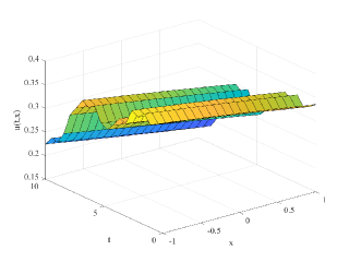
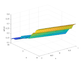
Figure 1. Two realizations of the stochastic process in equation (3.21).

Example 2.

Consider another stochastic KdV-Burgers equation

$$du = (\partial_{zzz}u+\partial_{zz}u+u\partial_{z}u)dt+\sigma(t)dW_{t},\quad$$ (3.22)

$$u(0,z) = \dfrac{3}{25}\operatorname{sech}^{2}\left(\frac{z}{10}\right)-\frac{6}{25}\tanh\left(\frac{z}{10}\right)+\frac{6}{25},$$ (3.23)

for $t\in[0,1]$. By Proposition 3 part (2), equation (3.31) has a solution

$$u(t,z)=V(t,Z_{t})+\dot{Z}_{t},$$

where $R(t)=1$, such that $V(t,x)$ is the solution of

$$\partial_{t}V = \partial_{xxx}V+\partial_{xx}V+V\partial_{x}V,$$ (3.24)

$$\quad V(0,z) = \dfrac{3}{25}\operatorname{sech}^{2}\left(\frac{z}{10}\right)-\frac{6}{25}\tanh\left(\frac{z}{10}\right)+\frac{6}{25},$$ (3.25)

and $Z_{t}$ is the solution of

$$\ddot{Z}_{t}=\sigma(t)\dot{W}_{t},$$ (3.26)

with initial state $Z_{0}=z$ and for $t\in[0,1]$.

Again, equation (3.32) has the general solution

$$V(t,z)=\dfrac{3}{25}\operatorname{sech}^{2}\left(\frac{z}{10}-\frac{6t}{250}\right)-\frac{6}{25}\tanh\left(\frac{z}{10}-\frac{6t}{250}\right)+\frac{6}{25}$$ (3.27)

for $z\in\mathbb{R}$. Also, $\dot{Z}_{t}=\int_{0}^{t}\sigma(r)dW_{r}$ due to Lemma 2. Thus, equation (3.31) has a solution

$$u(t,z)=\dfrac{3}{25}\operatorname{sech}^{2}\left(\frac{z+\int_{0}^{t}\sigma(s)dW_{s}}{10}-\frac{6t}{250}\right)-\frac{6}{25}\tanh\left(\frac{z+\int_{0}^{t}\sigma(s)dW_{s}}{10}-\frac{6t}{250}\right)+\frac{6}{25}+\int_{0}^{t}\sigma(r)dW_{r},$$ (3.28)

If  $\sigma(t)=1$, by Lemma 2, the stochastic differential equation (3.33) has a solution given by

$$Z_{t}=z-\int_{0}^{t}W_{s}ds$$

and  for $t\in[0,1].$

The general solution of the stochastic KdV-Burgers equation (3.31) is given by

$$u(t,z)=\dfrac{3}{25}\operatorname{sech}^{2}\left(\frac{z-\int_{0}^{t}W_{s}ds}{10}-\frac{6t}{250}\right)-\frac{6}{25}\tanh\left(\frac{z-\int_{0}^{t}W_{s}ds}{10}-\frac{6t}{250}\right)+\frac{6}{25}+\dot{Z}_{t}.$$ (3.29)

for $t\in[0,1]$ and $z\in\mathbb{R}$.

If  $\sigma(t)=t^{n}$, by Lemma 2, the stochastic differential equation (3.33) has a solution given by

$$Z_{t} = z-\int_{0}^{t}(t-s)s^{n}dW_{s}=z-t\int_{0}^{t}s^{n}dW_{s}+\int_{0}^{t}s^{n+1}dW_{s}$$

$$= z-t\left(t^{n}W_{t}-\int_{0}^{t}ns^{n-1}W_{s}ds\right)+t^{n+1}W_{t}-\int_{0}^{t}(n+1)s^{n}W_{s}ds.$$

and  for $t\in[0,1].$

In that case, the general solution of the stochastic KdV-Burgers equation (3.31) is given by

$$u(t,z)=\dfrac{3}{25}\operatorname{sech}^{2}\left(\frac{Z_{t}}{10}-\frac{6t}{250}\right)-\frac{6}{25}\tanh\left(\frac{Z_{t}}{10}-\frac{6t}{250}\right)+\frac{6}{25}+\dot{Z}_{t}$$ (3.30)

where $Z_{t}=z-t\left(t^{n}W_{t}-\int_{0}^{t}ns^{n-1}W_{s}ds\right)+t^{n+1}W_{t}-\int_{0}^{t}(n+1)s^{n}W_{s}ds,$ for $t\in[0,1]$ and $z\in\mathbb{R}$. Figure 2 shows two realizations of the general solution in (3.28).

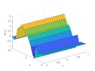
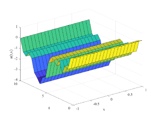
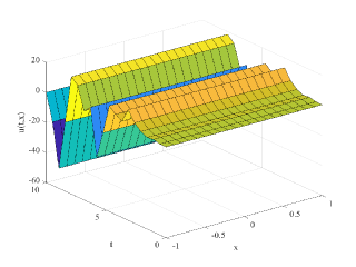
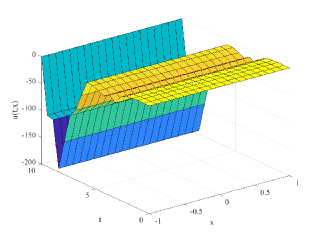
Figure 2. Four realizations of the stochastic process in equation (3.28) when $\sigma(t)=1$ (top) and $\sigma(t)=t^{2}$ (bottom).

Another example for the stochastic forced term is given here.

Example 3.

Consider another stochastic Burgers equation

$$du=(\exp(t)\partial_{zz}u+\exp(t)u\partial_{z}u)dt+dW_{t},\quad u(0,z)=\dfrac{2}{1+\exp(-2-z)}$$ (3.31)

for $t\in[0,1]$. By Proposition 3 part (2), equation (3.31) has a solution

$$u(t,z)=V(t,Z_{t})+\dfrac{1}{\exp(t)}\dot{Z}_{t},$$

where $R(t)=1$, such that $V(t,x)$ is the solution of

$$\partial_{t}V=\exp(t)\partial_{xx}V+\exp(t)V\partial_{x}V,\quad V(0,x)=\dfrac{2}{1+\exp(-2-x)}$$ (3.32)

and $Z_{t}$ is the solution of

$$\ddot{Z}_{t}=\dot{Z}_{t}+\exp(t)\dot{W}_{t},$$ (3.33)

with initial state $Z_{0}=z$ and for $t\in[0,1]$.

Again, equation (3.32) has the general solution

$$V(t,x)=\dfrac{2}{1+\exp(-1-x-\exp(t))}$$

for $x\in\mathbb{R}$.

By Lemma 2, the stochastic differential equation (3.33) has a solution given by

$$Z_{t}=z+\exp(t)W_{t}-\int_{0}^{t}\exp(s)dW_{s}$$

and

$$\dot{Z}_{t}=\exp(t)W_{t}$$

for $t\in[0,1].$

Therefore, the general solution of the stochastic Burgers equation (3.31) is given by

$$u(t,z)=W_{t}+\dfrac{2}{1+\exp(-1-z-\exp(t)-\exp(t)W_{t}+\int_{0}^{t}\exp(s)dW_{s})}$$ (3.34)

for $t\in[0,1]$ and $z\in\mathbb{R}$.

Figure 3 shows two realizations of the general solution in (3.34).

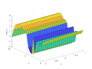
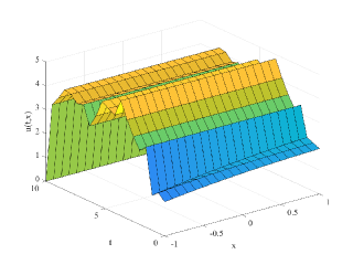
Figure 3. Two realizations of the stochastic process in equation (3.34).

4. Conclusion

In this paper, we showed using Itô calculus that some exact solutions of stochastic KdV-Burgers equations with several noise forms can be found using the deterministic KdV-Burgers equations. The exact solutions were introduced and simulated.

References

- [1] A. Alabert, I. Gyongy, On numerical approximation of stochastic Burgers’ equation, in: From Stochastic Calculus to Mathematical Finance, Springer, Berlin, Heidelberg, (2006), 1–15.
- [2] D.J. Benney, Long waves on liquid films, J. Math. Phys. 45 (1966) 150–155.
- [3] L. Bertini, N. Cancrini and G. Jona-Lasinio, The stochastic Burgers equation, Communications in Mathematical Physics, 165 (1994), 211–232.
- [4] L. Bertini and G. Giacomin, Stochastic Burgers and KPZ equations from particle systems, Communications in Mathematical Physics, 183 (1997), 571–607.
- [5] D. Blomker and A. Jentzen, Galerkin approximations for the stochastic Burgers equation, SIAM Journal of Numerical Analysis, 51 (2013), 694–715.
- [6] J. M. Burgers, A mathematical model illustrating the theory of turbulence, Advances in Applied Mechanics, 1 (1948), 171–199.
- [7] O. Calin, An Informal Introduction to Stochastic Calculus with Applications, World Scientific, 2015.
- [8] G. Casella and R. L. Berger, Statistical Inference, Duxbury advanced series in statistics and decision sciences, Thomson Learning, 2002.
- [9] P. Catuogno and C. Olivera, Strong solution of the stochastic Burgers equation, Applicable Analysis, 93 (2014), 646–652.
- [10] G. Da Prato, A. Debussche and R. Temam, Stochastic Burgers’ equation, Nonlinear Differential Equations and Applications, 1 (1994), 389–402.
- [11] P. Düben, D. Homeier, K. Jansen, D. Mesterhazy, G. Münster and C. Urbach, Monte Carlo simulations of the randomly forced Burgers equation, EPL Journal, 84 (2008), 1–4.
- [12] S. Eule and R. Friedrich, A note on the forced Burgers equation, Physics Letters A: General, Atomic and Solid State Physics, 351 (2006), 234–241.
- [13] S Flores, E Hight, E Olivares Vargas, T Oraby, J Palacio, E Suazo, J Yoon, Exact and numerical solution of stochastic Burgers equations with variable coefficients, Discrete and Continuous Dynamical Systems-S 13 (10), 2735-2750
- [14] G. Gao, A theory of interaction between dissipation and dispersion of turbulence, Sci. Sinica (Ser. A) 28 (1985) 616–627.
- [15] H. Grad, P.W. Hu, Unified shock profile in a plasma, Phys. Fluids 10 (1967) 2596–2602.
- [16] I. Gyöngy and D. Nualart, On the stochastic Burgers’ equation in the real line, The Annals of Probability, 27 (1999), 782–802.
- [17] M. Hairer and J. Voss, Approximations to the stochastic burgers equation, Journal of Nonlinear Science, 21 (2011), 897–920.
- [18] H. Holden, T. Lindstrøm, B. øksendal, J. Ubøe and T. Zhang, The Burgers equation with a noisy force and the stochastic heat equation, Communications in Partial Differential Equations, 19 (1994), 119–141.
- [19] P.N. Hu, Collisional theory of shock and nonlinear waves in a plasma, Phys. Fluids 15 (1972) 854–864.
- [20] R.S. Johnson, Shallow water waves on a viscous fluid—the undular bore, Phys. Fluids 15 (1972) 1693–1699.
- [21] T. Karahara, Weak nonlinear magneto-acoustic waves in a cold plasma in the presence of effective electron–ion collisions, J. Phys. Soc. Japan 27 (1970) 1321–1329.
- [22] P. E. Kloeden and E. Platen, Numerical Solution of Stochastic Differential Equations, Springer, Berlin, Heidelberg, 1992.
- [23] P. Lewis and D. Nualart, Stochastic Burgers’ equation on the real line: regularity and moment estimates, Stochastics, 90 (2018), 1053–1086.
- [24] E. Pereira, E. Suazo and J. Trespalacios, Riccati – Ermakov systems and explicit solutions for variable coefficient reaction – diffusion equations, Applied Mathematics and Computation, 329 (2018), 278–296.
- [25] A. Truman and H. Z. Zhao, On stochastic diffusion equations and stochastic Burgers’ equations, Journal of Mathematical Physics, 37 (1996), 283–307.
- [26] M. Wadati, Wave propagation in nonlinear lattice, J. Phys. Soc. Japan 38 (1975) 673–680.
- [27] E. Weinan, Stochastic hydrodynamics, Current Developments in Mathematics, (2000), 66p.
- [28] L. van Wijngaarden, On the motion of gas bubbles in a perfect fluid, Ann. Rev. Fluid Mech. 4 (1972) 369–373.