zju]School of Aeronautics and Astronautics, Zhejiang University, Hangzhou 310058, P. R. China nus]Department of Electrical and Computer Engineering, National University of Singapore, Singapore 117583, Singapore csu]School of Automation, Central South University, Changsha 410083, P. R. China hit]School of Mechanical Engineering and Automation, Harbin Institute of Technology, Shenzhen, Guangdong 518055, P. R. China
Low-cost adaptive obstacle avoidance trajectory control for express delivery drone
Abstract
This paper studies quadcopters’ obstacle avoidance trajectory control (OATC) problem for express delivery. A new nonlinear adaptive learning controller that is low-cost and portable to different wheelbase sizes is proposed to adapt to large-angle maneuvers and load changes in UAV delivery missions. The controller consists of a nonlinear variable gain (NLVG) function and an extreme value search (ES) algorithm to reduce overshoot and settling time. Finally, simulations were conducted on a quadcopter to verify the effectiveness of the proposed control scheme under two typical collision-free trajectories.
keywords:
Adaptive Learning Control, Delivery Drone, Obstacle Avoidance1 Introduction
The obstacle avoidance trajectory control (OATC) problem of the uncrewed aerial vehicle (UAV) has received significant attention recently in the real world (indoor and outdoor) as illustrated in [1]. In these scenarios, the drones that can avoid obstacles have more application value for many missions, such as exploration, swarms flight, and prevention-control of new coronavirus (see [2], [3], and references therein). Since drones are not limited by infrastructure such as light poles, streams, and walls, they can lower labor costs and reduce package delivery time [4]. Significantly, the demand for drone delivery tasks is increasing sharply, and it is vital to realize obstacle avoidance flight control in 3D airlines [5]. Hence, in the future scenario of dense air flight traffic, OATC between UAVs-UAVs and UAVs-MAVs (Manned Vehicle) will be sensitive.
In the last decades, several classical methodologies have been presented for OATC to achieve the flight control of quadcopters, such as detection and image processing in [6]. Also, for such UAV obstacle avoidance problems, some researchers have done some exciting work in the fields of motion planning for drones. Besides, some others focus on the controller problems, as our former work in [7] and W. Bao described in [8]. However, due to the varied layout and motors, quadcopters’ parameters are different in practical scenarios. Hence, the controller transplant cost must be lowered to adapt to another flight platform. Thus, the NN controllers have yet to be used on a large scale in recent years. In recent years, some methods have been proposed to solve the problem (such as PID, ESC [9]). Some others designed the control system combined PID/MPC with robust control and learning-based adaptive control in [10] and [11]. Motivated by the observation above, this paper proposes NLVG-PID, which could reduce the overshoot of fixed-gains PID controllers. The main contributions of this work lie in: The structure of the fixed-gain PID controller and the nonlinear dynamics and kinematics models are analyzed in this work. The NLVG-PID controller of a delivery quadcopter is designed, and the extremum seeking is introduced to learn the optimal nonlinear PID parameter under boundary conditions. To our knowledge, this is the first NLVG-PID obstacle avoidance controller to be used in delivery drones. A simulation was performed on a quadcopter to verify the effectiveness of the proposed control scheme under two typical collision-free trajectories.
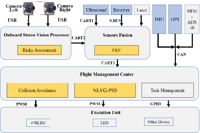
The Scheme of quadcopter control system is described in Fig. 1.
The remainder of this paper is organized as follows: Section 2, the mathematical model of dynamics, kinematics, and obstacle detection pipeline of the quadcopter are described in detail. In Section 3, the NLVG-PID framework and an ES method for boundary optimal parameter determination are developed. The stability analysis of the closed-loop system is also provided in this section. In Section 4, the quadcopter’s NLVG-PID controller system has been verified in four-side route, 8-character route, and scenic spiral position tracking, respectively. Section 5 concludes this work.
2 Problem formulation
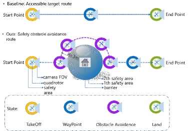
This paper assumes that the structure of the express delivery drone, an X-type quadcopter from [6], is known, but the specific load weight and the precise model of the drone are unknown. Obstacle avoidance is performed in three-dimensional space. First, the threat area is circled in the top view, as shown in Fig.2. Avoid obstacles, and then choose whether to fly upward or downward according to the distance cost in Euclidean space.
To facilitate the analysis of the rotation and translation of the UAV, a coordinate system is depicted as shown in our former work [12], the denotes the body-fixed coordinate system (B-frame), is the earth inertial frame (E-frame), indicates the velocity of quadcopter in E-frame. The schematic diagram of the quadcopter control system includes the following components, as displayed in Fig. 1.
3 Controller design
Usually, PID controller is defined as follows:
| (1) |
with and
| (2) |
, are the desired value and the real value of .
Remark 1
It can be observed that the quadcopter system is highly nonlinear and strongly coupled.
Remark 2
It can be seen that the quadcopter system is highly nonlinear and strongly coupled. Usually, in order to reduce the complexity of control system design, channel decoupling is used to decouple the three-axis position and attitude control.
3.1 NLVG-PID controller
Defining nonlinear variable gains of controller in channle . Besides, impact on .
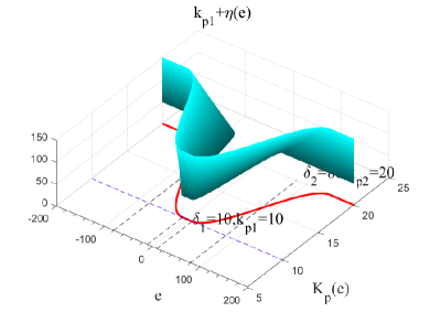
In order to improve the PID controller’s fast control capability for errors of different sizes, nonlinear gain terms are used instead of the fixed terms in (1). When the small error is close to zero, the value of the NLVG parameter reaches the lower limit . In the case of large errors, the upper limit is reached, as shown in Fig. 3. Hence, we design the control law as follows:
| (3) |
where
| (4) |
and
| (5) |
where , which based on the performance metrics (13), as shown in Fig. 3. Likewise, the integral item is
| (6) |
where
| (7) |
and the differential item is
| (8) |
where
| (9) |
Defining the state vector of the quadcopter as:
| (10) |
and the input vector of controller can be formulated as
| (11) | ||||
where , and
| (12) |
where , and. In (12), is the real value of , and is the desire value of .
3.2 ES in NLVG-PID
In ES, disturbance driving is used to find and maintain an extremum value for dynamic systems. This approach was first proposed by Leblanc, and the stability analysis of ES was first generally implemented by Krstic in [14]. We used the ES method to calculate the local optimal PID gain for the controller. The input is the step signal (e.g., maximum desired angle or position), while the output is the boundary of variable gains, where and . . The cost function of drone performance during the time can be defined as
| (13) |
where denotes the error in following the desired path with initial disturbance using parameters . Suppose the cost function gradient, , is available and could iteratively improve the parameter of the NLVG-PID controller. The parameter iterate rule can be defined as
| (14) |
where denotes the step size of the parameter of the quadcopter at each step of the iteration, and denotes the parameter vector after times iterations. Then the key point is to estimate . That is
| (15) |
From (13), the derivative to the gains numerically can be computed as
| (16) |
where is the unit vector in the direction. When , this approximation can minimize the cost function and optimize the local boundary PID parameters. The parameters are randomly initialized to positive numbers, and the periodic perturbation function is evaluated to evaluate the varying PID parameters and gradients of . To avoid the cost function falling into a local optimum, the initial value of the optimization value needs to be randomly reset multiple times and compared to find the best result. By plotting the functional relationship between the cost function and the number of iterations, we can observe the convergence of the system and verify the working principle of this learning method.
3.3 Strategy planning of obstacle avoidance
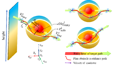
The stereo cameras are used to detect the largest threat in the visual range of the cameras, which fuse with distance from the ultrasonic sensor to the obstacles front at the visual risk assessment models. The relative position of the quadcopter is and the direction is . The denotes the distance of the current position and the boundary safety position of quadcopter , and the safety radius of the generated 3D sphere in intersecting line on the direction of the velocity vector, Bessel curve fitting is carried out by setting the trajectory of UAV that meets the dynamic constraints.
4 Simulation and results
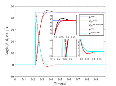
A simulation experiment was established to verify the efficiency of the NLVG-PID controller. The specific test parameters are set as [12]. The rate inner loop controller is the lowest-level controller of the quadcopter. Aiming at the internal loop angle control’s step response, PID control and NLVG-PID plus ES control simulation experiments were conducted. The results and analysis are shown in Fig. 5 and Table 1. It should be noted that the performance of the NLVG-PID controller uses three cost functions (IAE: integrated absolute error, ITAE: integration time and absolute error, ITSE: integrated time-weighted squared error), as set , .
| Channel | PID | NLVG-PID (Ours) | Function | |||||
| IAE | ITAE | ITSE | IAE | ITAE | ITSE | - | ||
| 1025.01 | 5.10 | 185.75 | 933.8 | 4.71 | 156.42 | attitude in x axis (o) | ||
| 1015.29 | 5.03 | 172.42 | 910.0 | 4.33 | 140.90 | attitude in y axis (o) | ||
| x | 94.82 | 0.47 | 0.92 | 86.32 | 0.43 | 0.78 | position x | |
| y | 91.82 | 0.41 | 0.89 | 82.66 | 0.36 | 0.70 | position y | |
| ∗ ; ; . | ||||||||
The initial parameters of the quadcopter can be determined as [6]. First, the inner loop controller parameters , , , and the outter loop position controller initial parameters are , , . Second, the scaler gains , , then the controller parameters are learned by ES in subsection 3.2. Moreover, the step size of this simulation is ; the total time is .
4.1 Example 1: Storm path following
To verify the effect of large-angle turning and small-angle adjustment of aircraft under the disturbance of obstacles, a storm airline is a continuous arc of increasing radius and height, designed as Fig. 6.
a) Storm-type obstacle avoidance routes in 3D view.
b) Storm-type obstacle avoidance routes in X-Y view.
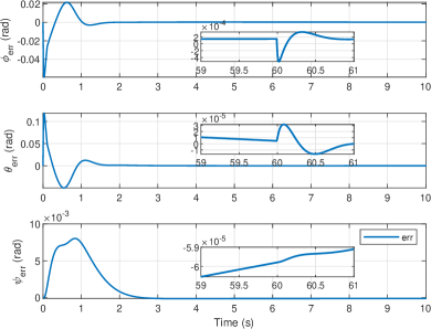
As shown in the Fig. 6-9, when the aircraft executes the takeoff command at t=20s, the attitude angle error is significant at this time. Then, PID and dynamic adaptive control algorithms are used for individual control. During the execution of the storm path, the attitude angle error decreases, and the control optimization effect is significantly improved.
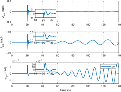
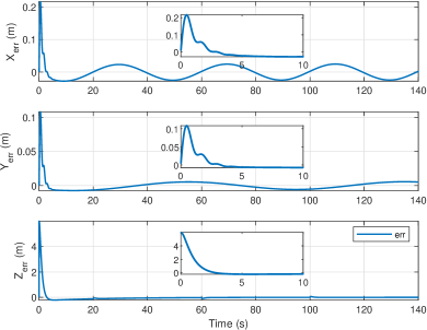
The Euler angle , the angle error , the position , and the position error in OATC are described in Fig. 6-9, respectively. From these figures, it can be observed that the angle and position errors can lead to a fast convergence into the local neighborhood areas in both the fixed-gain PID controller and NLVG-PID. However, the proposed NLVG-PID with ES control systems can perform well in OATC missions. It should be noted that the altitude of these missions is to keep the same value as .
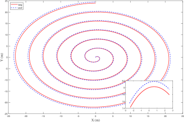
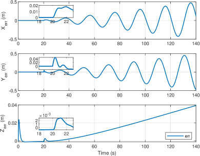
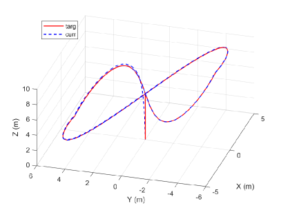
The desired trajectory path (Lissajous-type) of the quadcopter is depicted in Fig. 10, and the Euler angle and the position error in OATC are described in Fig. 10-14, respectively. As can be seen from these figures, using NLVG is better than PID in calculating a fast and smooth control output, thereby quickly tracking the desired command. It is worth noting that the height of this mission dynamically changes with the Lissajous-type path, which can verify that the proposed NLVG-PID performs well in periodic 3D path tracking.
4.2 Example 2: Lissajous curve following
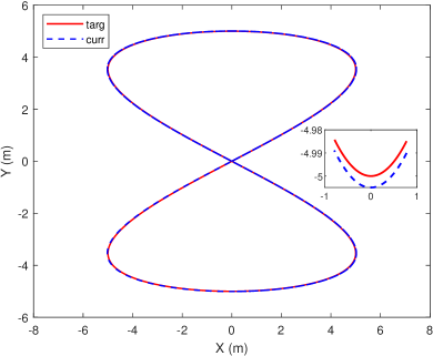
This work designed a 3D-Lissajous curve to conduct flight simulation verification of the quadcopter’s control performance under periodic disturbances.
a) Lissajous-type path in 3D view.
b) Lissajous-type path in X-Y view.
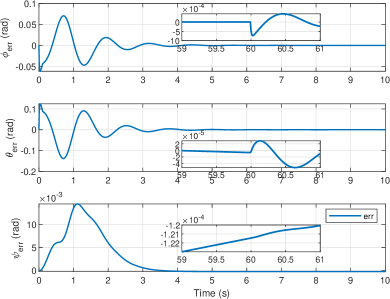
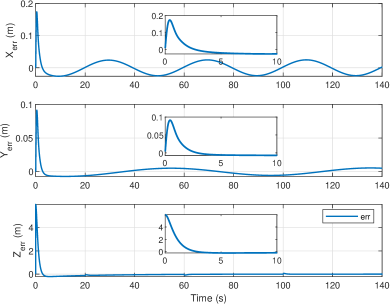
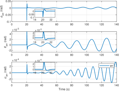
As can be seen in Fig. 12, when the aircraft executes the takeoff command at t=0s, the position and attitude angle errors at the moment of takeoff are significant. Then, PID and dynamic adaptive control algorithms are used for control, respectively. During the execution of the Lissajous path, the attitude angle error is gradually reduced by about 50%, the position error is reduced by about 15%, and the control optimization effect is partially improved. Compared with Example 4.1, the path of Example 4.2 is more complex, and there are significant changes in height and position, so the effect improvement is slightly reduced.
5 Conclusion
This paper studies the active motion control problem of quadcopter obstacle avoidance. A new design scheme for adaptive learning control of flight controllers based on low-cost dynamic linear optimization under uncertain conditions with obstacles is proposed. First, an NLVG-PID controller is presented for the formulated UAV model. Furthermore, ES is used to learn optimal NLVG-PID parameters in offline maximum or minimum error step signals. Numerical simulations were performed based on this design, and the results show that the proposed adaptive learning controller can reduce response overshoot and settling time in typical 3D path curves (such as storm paths).
References
References
- [1] S. Bouabdallah, P. Murrieri, and R. Siegwart, “Design and control of an indoor micro quadrotor,” IEEE International Conference on Robotics and Automation, 2004. Proceedings. ICRA 04. 2004, vol. 5, pp. 4393–4398 Vol.5, 2004.
- [2] Y. Chen, D. Huang, N. Qin, and Y. Zhang, “Adaptive iterative learning control for a class of nonlinear strict-feedback systems with unknown state delays,” IEEE Transactions on Neural Networks and Learning Systems, vol. 34, no. 9, pp. 6416–6427, 2023.
- [3] Y. Zhang, J. Sun, H. Liang, and H. Li, “Event-triggered adaptive tracking control for multiagent systems with unknown disturbances,” IEEE Transactions on Cybernetics, vol. 50, no. 3, pp. 890–901, 2020.
- [4] Q. Xu and Y. Zhang, “Event-triggered nonlinear information fusion preview control of a two-degree-of-freedom helicopter system,” Aerospace Science and Technology, vol. 140, p. 108474, 2023.
- [5] B. J. Emran and H. Najjaran, “A review of quadrotor: An underactuated mechanical system,” Annual Reviews in Control, vol. 46, pp. 165 – 180, 2018.
- [6] Y. Zhang, T. Chen, S. Chen, and Z. Wang, “Assess-ranging-fuse: Obstacle detection based on stereo vision threat assessment and ultrasonic ranging,” in 2020 Chinese Automation Congress (CAC), 2020, pp. 6186–6191.
- [7] Y. Zhang, Y. Yang, W. Chen, and H. Yang, “Realtime brain-inspired adaptive learning control for nonlinear systems with configuration uncertainties,” IEEE Transactions on Automation Science and Engineering, pp. 1–12, 2023.
- [8] W. Bao and Z. Qi, “Challenges and perspectives of information and control technology for cislunar space exploration and development,” Guidance, Navigation and Control, vol. 03, no. 02, p. 2350013, 2023.
- [9] C. Yin, Y. Chen, and S.-m. Zhong, “Fractional-order sliding mode based extremum seeking control of a class of nonlinear systems,” Automatica, vol. 50, no. 12, pp. 3173–3181, 2014.
- [10] Z. Xing, Y. Zhang, and C.-Y. Su, “Active wind rejection control for a quadrotor uav against unknown winds,” IEEE Transactions on Aerospace and Electronic Systems, vol. 59, no. 6, pp. 8956–8968, 2023.
- [11] C. Wei, J. Luo, H. Dai, and G. Duan, “Learning-based adaptive attitude control of spacecraft formation with guaranteed prescribed performance,” IEEE Transactions on Cybernetics, vol. 49, no. 11, pp. 4004–4016, 2019.
- [12] Y. Zhang, H. Yang, Y. Chen, and W. Chen, “Adaptive extremum seeking controller via nonlinear variable gain for uncertainty model multirotor,” in 2022 41st Chinese Control Conference (CCC), 2022, pp. 2308–2314.
- [13] N. J. Killingsworth and M. Krstic, “Pid tuning using extremum seeking: online, model-free performance optimization,” IEEE Control Systems Magazine, vol. 26, no. 1, pp. 70–79, 2006.
- [14] M. Krstic and H.-H. Wang, “Stability of extremum seeking feedback for general nonlinear dynamic systems,” Automatica, vol. 36, no. 4, pp. 595–601, 2000.