Coverage-Guaranteed Prediction Sets for Out-of-Distribution Data
Abstract
Out-of-distribution (OOD) generalization has attracted increasing research attention in recent years, due to its promising experimental results in real-world applications. In this paper, we study the confidence set prediction problem in the OOD generalization setting. Split conformal prediction (SCP) is an efficient framework for handling the confidence set prediction problem. However, the validity of SCP requires the examples to be exchangeable, which is violated in the OOD setting. Empirically, we show that trivially applying SCP results in a failure to maintain the marginal coverage when the unseen target domain is different from the source domain. To address this issue, we develop a method for forming confident prediction sets in the OOD setting and theoretically prove the validity of our method. Finally, we conduct experiments on simulated data to empirically verify the correctness of our theory and the validity of our proposed method.
1 Introduction
Recent years have witnessed the remarkable success of modern machine learning techniques in many applications. A fundamental assumption of most machine learning algorithms is that the training and test data are drawn from the same underlying distribution. However, this assumption is consistently violated in many practical applications. In reality, the test environment is influenced by a range of factors, such as the distributional shifts across photos caused by the use of different cameras in image classification tasks, the voices of different persons in voice recognition tasks, and the variations between scenes in self-driving tasks (Nagarajan, Andreassen, and Neyshabur 2021). As a result, there is now a rapidly growing body of research with a focus on generalizing to unseen target domains with the help of the source domains, namely OOD generalization (Shen et al. 2021).
Existing OOD generalization methods focus on improving worst-case performance on the target domains, i.e., improving the average test accuracy of the model on the worst target domain. However, in some systems that require high security (such as medical diagnosis), even a single mistake may have disastrous consequences. In these cases, it is important to quantify the uncertainty of the predictions. One way to perform uncertainty estimation (Amodei et al. 2016; Jiang et al. 2012, 2018; Angelopoulos et al. 2021) is to create confident prediction sets that provably contain the correct answer with high probability. Let be a new test example for which we would like to predict the corresponding label , where is the input space and is the label space. For any given , the aim of confidence set prediction is to construct a set-valued output, , which contains the label with distribution-free marginal coverage at a significance level , i.e., . A confidence set predictor is said to be valid if for any , where is a hyper-parameter of the predictor. To simplify the notation, we omit the superscript in the remainder of this paper.
Conformal prediction (Vovk, Gammerman, and Shafer 2005; Shafer and Vovk 2008, CP) is a model-agnostic, non-parametric and distribution-free (the coverage guarantee holds for any distribution) framework for creating confident prediction sets. Split conformal prediction (Vovk 2013; Vovk, Gammerman, and Shafer 2005, SCP), a special type of CP, has been shown to be computationally efficient. SCP reserves a set of data as the calibration set, and then uses the relative value of scores of the calibration set and that of a new test example to construct the prediction set. The validity of SCP relies on the assumption that the examples are exchangeable. However, in the OOD setting, the distributional shift between the training and test distributions leads to the violation of the exchangeability assumption. We empirically evaluate the performance of SCP in the OOD setting in Section 4. Unfortunately, we find that trivially applying SCP results in a failure to maintain marginal coverage in the OOD setting.
To address this issue, we construct a set predictor based on the -divergence (Alfréd 1961) between the test distribution (target domain) and the convex hull of the training distributions (source domains). We theoretically show that our set predictor is guaranteed to maintain the marginal coverage (Corollary 9). We then conduct simulation experiments to verify our theory.
The remainder of this article is structured as follows: §2 introduces some related works; §3 presents the notation definitions and preliminaries; §4 conducts experiments that show the failure of SCP in the OOD generalization setting; §5 creates corrected confidence set predictor in the OOD generalization setting; §6 provides our experimental results. §7 make discussions with the most related work. Finally, the conclusions are presented in §8. All of our proofs are attached in Appendix A.
2 Related Works
OOD generalization. OOD generalization aims to train a model with data from the source domains so that it is capable of generalizing to an unseen target domain. A large number of algorithms have been developed to improve OOD generalization. One series of works focuses on minimizing the discrepancies between the source domains (Li et al. 2018b; Ganin et al. 2016; Li et al. 2018c; Sun and Saenko 2016). Meta-learning domain generalization (Li et al. 2018a, MLDG) leverages the meta-learning approach and simulates train/test distributional shift during training by synthesizing virtual testing domains within each mini-batch. Another line of works (Xin et al. 2022; Wang et al. 2022) conducts adversarial training (Madry et al. 2018) to improve the OOD generalization performance. (Zou and Liu 2023) considers improving the adversarial robustness of the unseen target domain. Notably, the above works all focus on improving the average performance on the target domain; in contrast, we focus on designing valid confidence set predictors for data from the unseen target domains, as this is a crucial element of making high-stakes decisions in systems that require high security.
Conformal prediction. As introduced in §1, conformal prediction is a model-agnostic, non-parametric, and distribution-free framework that provides valid confidence set predictors. Generally speaking, examples are assumed to be exchangeable in a CP context. Most pertinent to our work, (Gendler et al. 2022; Tibshirani et al. 2019; Fisch et al. 2021; Cauchois et al. 2020; Gibbs and Candès 2021; Oliveira et al. 2022) all consider various situations in which the exchangeability of the examples is violated to some extent. (Gendler et al. 2022) considers the case in which the test examples may be adversarially attacked (Szegedy et al. 2014; Goodfellow, Shlens, and Szegedy 2015; Madry et al. 2018); (Tibshirani et al. 2019) investigates the situation in which the density ratio between the target domain and the source domain is known; (Fisch et al. 2021) studies the few-shot learning setting and assumes that the source domains and the target domain are independent and identically distributed (i.i.d.) from some distribution on the domains; (Gibbs and Candès 2021) considers an online learning setting and (Oliveira et al. 2022) provides results when the examples are mixing (Achim 2013; Xiaohong, Lars Peter, and Marine 2010; Bin 1994). Different from all the works discussed above, we consider the OOD generalization setting in which the -divergence between the target domain and the convex hull of the source domains is constrained. The most related work among them is (Cauchois et al. 2020), which studies the worst-case coverage guarantee of a -divergence ball centered at the single source domain. For the discussions about similarities and differences with (Cauchois et al. 2020), please refer to Section 7.
3 Preliminaries
We begin with the OOD setups and a review of conformal prediction.
Notations. We denote by for . For a distribution on , we define the quantile function of as . Similarly, for a cumulative distribution function (c.d.f.) on , we define . For distributions , we define as the convex hull of the distributions . We further define as the multi-variable Gaussian distribution with mean vector and covariance matrix . For a set , we define the indicator function as , where if and otherwise.
3.1 Out-of-Distribution Generalization
We define the input space as and the label space as . We set , (where is the number of classes), and for the binary classification problem, the multi-class classification problem, and the regression problem, respectively. Let be the set of source domains, where is the number of source domains. are distributions on , and we use the terminologies ”domain” and ”distribution” interchangeably in this paper. Let denote the target domain. The goal of OOD generalization is to obtain good performance on all , where is the set of all possible target domains; we usually assume .
In a standard OOD generalization setting, we learn a predictor from the source domains and define a loss function where . We aim to minimize the worst-case population risk of the predictor on the unseen target domain as follows:
However, in some systems that require high security, a mistake may lead to serious disasters. In these cases, a good solution is to output a prediction set with a marginal coverage guarantee. For a predefined confidence level , we wish to output a prediction set such that, for any :
| (1) |
where the probability is over the randomness of test examples and the randomness of the prediction set . To achieve (1), we follow the idea of SCP (Vovk 2013; Vovk, Gammerman, and Shafer 2005) to construct . The next section introduces the main idea of SCP.
3.2 Split Conformal Prediction
Nonconformity score. In SCP, we consider a supervised learning problem that involves predicting the label of the input . We assume that we have a predictive model , which outputs the nonconformity score . The nonconformity score function is usually trained with a set of training data. means that for the input , is more likely than to be the label. Some examples of nonconformity scores are as follows: for a probabilistic model , we can take the negative log-likelihood as the score, ; for a regression model , a typical choice is ; for a multi-class classifier , where is the dimensional simplex in , we can take .
In SCP, we assume that the examples are exchangeable (Definition 1). For a predefined significance level , the goal is to provide a valid confidence set . CP methods (Shafer and Vovk 2008) take advantage of the exchangeability of the data and the properties of the quantile function to make such a construction possible.
Definition 1 ((Shafer and Vovk 2008, Exchangeability)).
The random variables are exchangeable if for every permutation for integers , the variables , where , have the same joint probability distribution as .
Let for be the nonconformity scores corresponding to the examples , where is independent of . The independence between and is useful since in this case we can prove that the scores are exchangeable. The exchangeability of comes from the exchangeability of and the independence between the and . Next, define as the rank of among for any (in ascending order; we assume that ties are broken randomly). By the exchangeability of , is uniform on , which is used to prove the validity of SCP in Lemma 2. We use to denote the empirical distribution determined by the examples . Let
| (2) |
we then have the following marginal coverage guarantee.
Lemma 2 (The validity of SCP).
Assume that examples are exchangeable. For any nonconformity score and any , the prediction set defined in Equation 2 satisfies:
| (3) |
where the probability is over the randomness of .
In the OOD generalization setting, we also want to obtain a valid set predictor that is valid for any . In light of this, some natural questions arise:
Does the set predictor defined in Equation 2 remain valid when the unseen target domain is different from the source domains? If not, can we construct a new set predictor that is valid in the OOD generalization setting?
Unfortunately, the answer to the first question is negative. Theoretically, as shown in Appendix A.1, the proof of Lemma 2 is highly dependent on the exchangeability of the examples , which is easily violated if there is any distributional shift between the distribution of and the distribution of . This means that in the OOD setting, the proof technique of Lemma 2 cannot be applied. Empirically, in Section 4, we provide a toy example to show that the set predictor is no longer valid in the OOD setting.
In Section 5, we give an affirmative answer to the second question. We first construct a new set predictor based on the -divergence between the target domain and the convex hull of the source domains, then provide marginal coverage guarantees for the constructed predictor.
4 SCP Fails in the OOD Setting
In this section, we construct a toy example to show that for the OOD confidence set prediction problem, SCP is no longer valid, even under a slight distributional shift.
For simplicity, we consider a single-domain case. Specifically, we consider the regression problem and set , . We define the source domain as follows: given a linear predictor where and . The marginal distribution of and the conditional distribution of given are defined as:
where is the mean vector of , are positive scalars, and is an identity matrix. Similarly, for the target domain , we define:
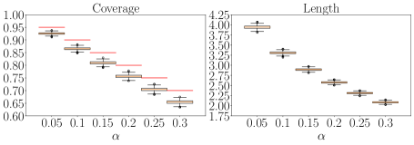
where is the mean vector of and are positive scalars. For simplicity, we set and . We sample training examples from to train a linear predictor , where and . We then define the nonconformity score as . We sample examples from to construct the prediction set in Equation 2 and sample examples from to form the test data. We run times with different random seeds. The results for the coverage (left) and length (right) of the prediction set are presented in box plot form in Figure 1. Here, the coverage is the ratio between the number of test examples such that and the size of the test set. The red lines stand for the desired marginal coverages. Since the boxes are below the red coverage lines, we conclude that SCP fails to provide a prediction set with desired coverage when there exists a distributional shift between the source domain and the target domain.
5 Corrected SCP for OOD Data
In this section, we consider correcting SCP for OOD data. We first consider the case in which we have access to the population distributions of the scores from the source domains. We then consider the case in which we only have access to the empirical distributions and correct the prediction set to obtain a marginal coverage guarantee in Equation 3.
5.1 Target Distribution Set and Confidence Sets
It is obvious that obtaining a marginal coverage guarantee for an arbitrary target distribution is impossible unless we set for all , which is a trivial confidence set predictor and does not provide any useful information. In this paper, we consider the case in which the -divergence (Alfréd 1961) between the target domain and the convex hull of the source domains does not exceed a predefined value. The well-known KL divergence and TV distance are both special cases of -divergence.
As Section 4 shows, when the target domain differs from the source domain, the marginal coverage does not hold for the predictor (2). Below, we construct new prediction sets where the marginal coverage (3) holds.
We define a set of distributions . For each , the distribution of the score for the data from is defined as the push forward distribution , where for any measurable set . We define the distribution set of the scores as . For a given , our goal is to choose a threshold such that the confidence set satisfies (3) when is drawn from any target domain . The following lemma provides a proper choice of .
Lemma 3.
For any unknown target distribution , assume that is drawn from . If we set , then:
| (4) |
For a given set of distributions for the score, Lemma 3 reduces the problem of finding a valid confidence set predictor to the following optimization problem:
| (5) |
Next, we formulate the set through the lens of -divergence.
Definition 4 (-divergence).
Let be a closed convex function satisfying and for . Let be two probability distributions such that ( is absolutely continuous with respect to ). The -divergence between and can then be defined as follows:
where is the Radon-Nikodym derivative (Patrick 2008).
Remark 1.
For a given function that satisfies the conditions in Definition 4, define . We then obtain that, for any :
By the convexity of , it can be easily observed that for all . Moreover, and . Since produces the same -divergence as , without loss of generality, we can assume that and .
Equipped with the -divergence, we can now define our target distribution set for a given threshold :
We omit and use for simplicity. The corresponding distribution set for the scores is then:
| (6) |
However, it is hard to obtain the precise relationship between and the distributions , which makes it difficult to analyze . We instead consider the following distribution set of scores:
| (7) | ||||
The following lemma reveals the relationship between and .
Remark 2.
According to Remark 2, we define the worst-case quantile function for the distribution set as . Remark 2 tells us that taking produces a valid confidence set . The next theorem allows us to express the worst-case quantile function in terms of the standard quantile function, which helps us to calculate the worst-case quantile efficiently.
Theorem 6.
Let be the c.d.f.’s of the distributions . Define the function as
and define the inverse of as . Let be a c.d.f., the following holds for all :
5.2 Marginal Coverage Guarantee for Empirical Source Distributions
In the previous section, we presented marginal coverage guarantees when we have access to the population distributions of the scores for source domains. However, in practice, it is difficult or even impossible to access these population distributions. In this section, we provide marginal coverage guarantees even when we only have access to the empirical distributions, which is useful in practice.
For any , assume we have i.i.d. examples from the source distribution . Further, suppose that is the empirical c.d.f. corresponding to , which is defined as . Define . We first provide an error bound when we estimate with .
Proposition 7.
Let be c.d.f.’s on , define . Suppose are the empirical c.d.f.’s corresponding to , defined with examples, respectively. Define . Then, for any ,
where the probability is over the randomness of the examples that define the empirical c.d.f.’s.
The above Proposition 7 allows us to quantify the error caused by replacing the population distributions with the empirical distributions, which leads to the following marginal coverage guarantee for the prediction set that we have defined before.
Theorem 8 (Marginal coverage guarantee for the empirical estimations).
Assume is independent of where for . Suppose where . Let be defined as in Proposition 7 and let be the empirical distributions of respectively. If we set , then for any , we obtain the following marginal coverage guarantee for :
where the randomness is over the choice of the source examples and and
By Lemma 14 in the Appendix, is non-increasing in and non-decreasing in , so . In practice, we do not know , so we use instead. Since , we get guaranteed coverage . To achieve a marginal coverage with the level of at least , we need to correct the output set by replacing with some when running our confidence set predictor. The following corollary tells us how to choose to correct the prediction set.
Corollary 9 (Correct the prediction set to get a marginal coverage).
Let , , be defined as in Theorem 8. For arbitrary , if we set , where
then we obtain the following marginal coverage guarantee:
Remark 3.
Corollary 9 tells us that we can take to get a marginal coverage guarantee with confidence level . When are chosen and the numbers of examples that are used to estimate the source distributions, i.e., , are given, we solve the following optimization problem to find a desired .
| s.t. |
Since the quantile function is non-decreasing, let , we solve the following problem instead:
For some choices of , the functions and have closed forms (please refer to the examples in Section 5.3). For general that we do not have a closed form of , the following lemma tells us that we can use a binary search algorithm to efficiently compute the value of for a given .
5.3 Examples
In this section, we present some examples of calculating and for some important -divergences.
Example 1 (-divergence).
Let ; then, is the -divergence. In this case, we have , where . is the solution of the following optimization problem:
Example 2 (Total variation distance, (Cauchois et al. 2020)).
Let ; then, is the total variation distance. In this case, we can provide analytic forms for and :
Example 3 (Kullback-Leibler divergence).
Let ; then, is the Kullback-Leibler (KL) divergence (Solomon and Richard A 1951). Unfortunately, we cannot provide the analytic forms of and for KL-divergence. Fortunately, according to Theorem 6 and Remark 3, we can compute the values and by solving a one-dimensional convex optimization problem, which can be solved efficiently using binary search.
6 Experiments
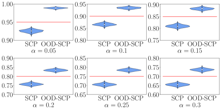
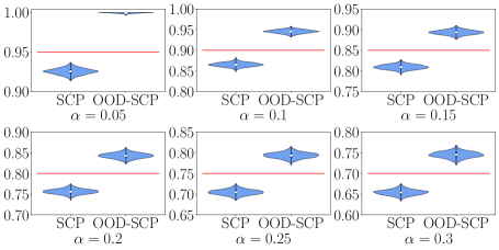
In this section, we use simulated data to verify our theory and the validity of our constructed confidence set predictor (referred to as OOD-SCP in the remainder of this paper). We consider two cases: first, we verify the validity of OOD-SCP using the same settings as in Section 4; then, we construct a multi-source OOD confidence set prediction task and show that OOD-SCP is valid for this task.
According to Figure 2, unlike standard SCP, for all values of , the violin for OOD-SCP is above the desired coverage line, which shows that OOD-SCP is empirically valid.
We next consider a multi-source OOD confidence set prediction task. Similar to Section 4, we consider the regression problem and set . Define the oracle linear predictor as , where and . We define the marginal distribution of for the source domains and as
respectively, where are the mean vectors, is a scalar, and is the identity matrix with dimension . We define for both and . For the target domain , we define the marginal distribution of as and the conditional distribution of given as . Here, are the standard deviations and .
Similar to Section 4, we sample examples from and examples from to train a linear predictor , where and . We then define the nonconformity score as . We sample examples from , and examples from to construct the prediction set and sample examples from to form the test data.
Figure 3 shows the results for the multi-source OOD confidence set prediction task. From the figure, we can see that the violins for the standard SCP are under the desired coverage lines, which means that the standard SCP is invalid in this case. By contrast, the violins for OOD-SCP are above the desired coverage lines, indicating that OOD-SCP is valid, which validates Corollary 9.
The reason we do not do experiments on real datasets is that do not know how to set the value of for the existing OOD datasets. Our main claim is that when the target domain satisfies , the coverage of our method is guaranteed. However, we claim it is acceptable. In many fields, we face the same problem.
In adversarial robustness (Szegedy et al. 2014), the theories (for example (Montasser, Hanneke, and Srebro 2019)) provide an upper bound of the test adversarial robustness , where is a classifier. The results just tell us that we have the guarantee for the test accuracy if the test perturbation satisfies . However, what if ? It is out of the scope of their theories.
For distributional robustness optimization (DRO), the theories (Lee and Raginsky 2018) prove that if the test distribution is in a Wasserstein ball with radius , then the test risk can be upper bounded. Formally, is upper bounded, where is a Wasserstein ball with radius. They do not know how to set to make contain the test distribution either, however, this does not overshadow their contribution to the DRO community. In other words, the issues of do not overshadow our contribution to the OOD community.
7 Discussions
Our work is an extension of (Cauchois et al. 2020) to the multi-domain case. In this section, we discuss the differences between our work and (Cauchois et al. 2020).
7.1 The Necessity of Our Extension
In the multi-source setting, to make use of all the source domains, a trivial method is to regard the mixture of the source domains, as a domain and use the method in (Cauchois et al. 2020). However, there are two issues:
-
•
Given the empirical data from , we don’t know the exact values of for the mixed domain, so we don’t know the set for a given . So we don’t know the set that we are giving a coverage guarantee for.
-
•
We may be not able to provide a coverage guarantee for data from one of the source domains. Take KL-divergence as an example, then drawing from can be regarded as first drawing an index from and then drawing an example from . can be seen as drawn from the same process with , where with only the -th element being . By the chain rule, . If , then there exists a s.t. , i.e., we can not even get a coverage guarantee for the source domain , which is unacceptable! The problem gets worse if the source domain number becomes larger since . However, in our generalization, there is no such problem even if we choose , which means the method in (Cauchois et al. 2020) is not compatible with the multi-source setting, so our extension is necessary.
7.2 The Difference in Proof Skills
In fact, our Theorem 6 is an extension of (Cauchois et al. 2020) to the OOD setting and mainly depends on Lemmas 17 and 18. Lemma 17 helps us reduce multi-input to a single-input case. The main idea of the proof of Lemma 18 comes from the argument in (Cauchois et al. 2020), however, the extension is non-trivial. In Lemma 18, let we use the multi-input , which involves taking infimum w.r.t. and is much more complicated than the single-input case in (Cauchois et al. 2020). We construct a set that is more complicated than that in (Cauchois et al. 2020) and the proof is more difficult. Moreover, due to multiple inputs and the operator, we need to consider 4 cases according to whether each is or .
Our Theorem 8 and its corresponding Corollary 9 are novel and quite different from Corollaries 2.1 and 2.2 in (Cauchois et al. 2020). The common point is that they all consider finite sample approximation. The proof of Corollary 2.1 in (Cauchois et al. 2020) relies on the exchangeability of the source examples, however, in the OOD setting, examples are drawn from different source domains and are not exchangeable. So the analysis techniques in (Cauchois et al. 2020) can not be applied in our case. To fill this gap, we use the decomposition technique and concentration inequalities.
8 Conclusion
We study the confidence set prediction problem in the OOD generalization setting. We first empirically show that SCP is not valid in the OOD generalization setting. We then develop a method for forming valid confident prediction sets in the OOD setting and theoretically prove the validity of our proposed method. Finally, we conduct experiments on simulated data to empirically verify both the correctness of our theory and the validity of our proposed method.
Acknowledgements
This work is supported by the National Key R&D Program of China under Grant 2023YFC3604702, the National Natural Science Foundation of China under Grant 61976161, the Fundamental Research Funds for the Central Universities under Grant 2042022rc0016.
References
- Achim (2013) Achim, K. 2013. Probability theory: a comprehensive course. Springer Science & Business Media.
- Alfréd (1961) Alfréd, R. 1961. On measures of entropy and information. In Proceedings of the Fourth Berkeley Symposium on Mathematical Statistics and Probability, Volume 1: Contributions to the Theory of Statistics, volume 4, 547–562.
- Amodei et al. (2016) Amodei, D.; Olah, C.; Steinhardt, J.; Christiano, P. F.; Schulman, J.; and Mané, D. 2016. Concrete Problems in AI Safety. CoRR, abs/1606.06565.
- Angelopoulos et al. (2021) Angelopoulos, A. N.; Bates, S.; Jordan, M. I.; and Malik, J. 2021. Uncertainty Sets for Image Classifiers using Conformal Prediction. In ICLR.
- Bin (1994) Bin, Y. 1994. Rates of convergence for empirical processes of stationary mixing sequences. The Annals of Probability, 94–116.
- Boyd, Boyd, and Vandenberghe (2004) Boyd, S.; Boyd, S. P.; and Vandenberghe, L. 2004. Convex optimization. Cambridge university press.
- Cauchois et al. (2020) Cauchois, M.; Gupta, S.; Ali, A.; and Duchi, J. C. 2020. Robust Validation: Confident Predictions Even When Distributions Shift. CoRR, abs/2008.04267.
- Fisch et al. (2021) Fisch, A.; Schuster, T.; Jaakkola, T. S.; and Barzilay, R. 2021. Few-Shot Conformal Prediction with Auxiliary Tasks. In ICML, 3329–3339.
- Ganin et al. (2016) Ganin, Y.; Ustinova, E.; Ajakan, H.; Germain, P.; Larochelle, H.; Laviolette, F.; Marchand, M.; and Lempitsky, V. S. 2016. Domain-Adversarial Training of Neural Networks. J. Mach. Learn. Res., 17: 59:1–59:35.
- Gendler et al. (2022) Gendler, A.; Weng, T.; Daniel, L.; and Romano, Y. 2022. Adversarially Robust Conformal Prediction. In ICLR.
- Gibbs and Candès (2021) Gibbs, I.; and Candès, E. J. 2021. Adaptive Conformal Inference Under Distribution Shift. In NeurIPS, 1660–1672.
- Goodfellow, Shlens, and Szegedy (2015) Goodfellow, I. J.; Shlens, J.; and Szegedy, C. 2015. Explaining and Harnessing Adversarial Examples. In ICLR.
- Jiang et al. (2018) Jiang, H.; Kim, B.; Guan, M. Y.; and Gupta, M. R. 2018. To Trust Or Not To Trust A Classifier. In NeurIPS, 5546–5557.
- Jiang et al. (2012) Jiang, X.; Osl, M.; Kim, J.; and Ohno-Machado, L. 2012. Calibrating predictive model estimates to support personalized medicine. J. Am. Medical Informatics Assoc., 19(2): 263–274.
- Lee and Raginsky (2018) Lee, J.; and Raginsky, M. 2018. Minimax Statistical Learning with Wasserstein distances. In NeurIPS, 2692–2701.
- Li et al. (2018a) Li, D.; Yang, Y.; Song, Y.; and Hospedales, T. M. 2018a. Learning to Generalize: Meta-Learning for Domain Generalization. In AAAI, 3490–3497.
- Li et al. (2018b) Li, H.; Pan, S. J.; Wang, S.; and Kot, A. C. 2018b. Domain Generalization With Adversarial Feature Learning. In CVPR, 5400–5409.
- Li et al. (2018c) Li, Y.; Tian, X.; Gong, M.; Liu, Y.; Liu, T.; Zhang, K.; and Tao, D. 2018c. Deep Domain Generalization via Conditional Invariant Adversarial Networks. In ECCV, volume 11219, 647–663.
- Madry et al. (2018) Madry, A.; Makelov, A.; Schmidt, L.; Tsipras, D.; and Vladu, A. 2018. Towards Deep Learning Models Resistant to Adversarial Attacks. In ICLR.
- Massart (1990) Massart, P. 1990. The tight constant in the Dvoretzky-Kiefer-Wolfowitz inequality. The annals of Probability, 1269–1283.
- Montasser, Hanneke, and Srebro (2019) Montasser, O.; Hanneke, S.; and Srebro, N. 2019. VC Classes are Adversarially Robustly Learnable, but Only Improperly. In COLT, 2512–2530.
- Nagarajan, Andreassen, and Neyshabur (2021) Nagarajan, V.; Andreassen, A.; and Neyshabur, B. 2021. Understanding the failure modes of out-of-distribution generalization. In ICLR.
- Oliveira et al. (2022) Oliveira, R. I.; Orenstein, P.; Ramos, T.; and Romano, J. V. 2022. Split Conformal Prediction for Dependent Data. arXiv:2203.15885.
- Patrick (2008) Patrick, B. 2008. Probability and measure. John Wiley & Sons.
- Shafer and Vovk (2008) Shafer, G.; and Vovk, V. 2008. A Tutorial on Conformal Prediction. J. Mach. Learn. Res., 9: 371–421.
- Shen et al. (2021) Shen, Z.; Liu, J.; He, Y.; Zhang, X.; Xu, R.; Yu, H.; and Cui, P. 2021. Towards Out-Of-Distribution Generalization: A Survey. CoRR, abs/2108.13624.
- Solomon and Richard A (1951) Solomon, K.; and Richard A, L. 1951. On information and sufficiency. The annals of mathematical statistics, 22(1): 79–86.
- Sun and Saenko (2016) Sun, B.; and Saenko, K. 2016. Deep CORAL: Correlation Alignment for Deep Domain Adaptation. In ECCV, volume 9915, 443–450.
- Szegedy et al. (2014) Szegedy, C.; Zaremba, W.; Sutskever, I.; Bruna, J.; Erhan, D.; Goodfellow, I. J.; and Fergus, R. 2014. Intriguing properties of neural networks. In ICLR.
- Tibshirani et al. (2019) Tibshirani, R. J.; Barber, R. F.; Candès, E. J.; and Ramdas, A. 2019. Conformal Prediction Under Covariate Shift. In NeurIPS, 2526–2536.
- Vovk (2013) Vovk, V. 2013. Conditional validity of inductive conformal predictors. Mach. Learn., 92(2-3): 349–376.
- Vovk, Gammerman, and Shafer (2005) Vovk, V.; Gammerman, A.; and Shafer, G. 2005. Algorithmic Learning in a Random World. Springer-Verlag. ISBN 0387001522.
- Wang et al. (2022) Wang, Q.; Wang, Y.; Zhu, H.; and Wang, Y. 2022. Improving Out-of-Distribution Generalization by Adversarial Training with Structured Priors. CoRR, abs/2210.06807.
- Xiaohong, Lars Peter, and Marine (2010) Xiaohong, C.; Lars Peter, H.; and Marine, C. 2010. Nonlinearity and temporal dependence. Journal of Econometrics, 155: 155–169.
- Xin et al. (2022) Xin, S.; Wang, Y.; Su, J.; and Wang, Y. 2022. Domain-wise Adversarial Training for Out-of-Distribution Generalization.
- Zou and Liu (2023) Zou, X.; and Liu, W. 2023. On the Adversarial Robustness of Out-of-distribution Generalization Models. In Thirty-seventh Conference on Neural Information Processing Systems.
Appendix A Proofs
A.1 Proof of Lemma 2
Lemma 2.
Assume that examples are exchangeable. For any nonconformity score and any , the prediction set defined in Equation 2 satisfies:
where the probability is over the randomness of .
Proof of Lemma 2.
Let , then the following holds:
where is from the definition of and is a result of the definition of the quantile function , the inner probability is over the randomness of and the outer probability is over the randomness of . ∎
A.2 Proof of Lemma 3
Lemma 3.
For any unknown target distribution , assume that is drawn from . If we set , then:
Proof of Lemma 3.
where is from the fact ; is because and is a result of the definition of the quantile function. ∎
A.3 Proof of Lemma 5
The proof of Lemma 5 relies on the data processing inequality for -divergence.
Lemma 11 (Data Processing Inequality for -divergence).
Let be distributions on measurable space and be a transition kernel from to . Let be distributions on measurable space and be the transformation of pushed through , i.e., . Then, for any f-divergence, we have that:
To prove Lemma 11, we need some properties about the -divergences.
Lemma 12 (Properties of -divergences).
For any distributions on dominated by a common measure , i.e. (such a always exists since we can take ), we have:
-
•
Non-Negativity: . Furthermore, if is strictly convex around , then the equality is obtained if and only if .
-
•
Convexity: The mapping is jointly convex. Consequently, is convex for fixed , and is convex for fixed .
-
•
Joint vs. Marginal: If and , then .
Proof of Lemma 12.
To prove the non-negativity, by the definition of -divergence we have:
where follows from Jensen’s inequality. Next, we prove that if is strictly convex around , then the equality is obtained if and only if . It is obvious that if , then , so . For the other direction, as stated in Remark 1, we assume , so implies that almost everywhere. Since in strongly convex around and , then implies , which means that .
To prove the convexity, let , for , we define as:
Since is convex, according to (Boyd, Boyd, and Vandenberghe 2004, Section 3.2.6, Page 89), is also convex. Denote , let be the domain of , for , suppose that (such exists, e.g., we can set ). Then, for any we have:
where is from the convexity of .
To prove the relationship between -divergence of joint distributions and marginal distributions, we have:
∎
A.4 Proof of Theorem 6
Theorem 6.
Let be the c.d.f.’s of the distributions . Define the function as:
then for inverse of :
the following holds for all :
where is a c.d.f.
Firstly, we prove that if are c.d.f.’s, then is a c.d.f.
Lemma 13.
Suppose that are c.d.f.’s, let , then is a c.d.f.
Proof of Lemma 13.
We need to prove that satisfies the following properties:
-
P1
is non-decreasing.
-
P2
, and .
-
P3
is right continuous.
Proof of P1: Since are all c.d.f.’s, , we have for all .
Suppose , then . Since , we have that:
which means that the function is non-decreasing.
Proof of P2: Since are all c.d.f.’s, then , for all . It is obvious that .
Since , , there exists such that , we have , i.e., . Let , then, if , holds for all , so , which means that . We can prove that similarly.
Proof of P3: Since are all c.d.f.’s, they are all right continuous. Fix any , then by the definition of right continuity, we know that: , , there exists such that, for any satisfying , we have:
Let , set , , then:
So, for all , we have:
Similarly, we have:
So we have that ∎
We now show some useful properties for , which are useful in our proof.
Lemma 14 (Lemma A.1, page 33 of (Cauchois et al. 2020)).
Let be a function that satisfies the conditions in Definition 4, then the function defined in Theorem 6 satisfies the following properties:
-
(1)
The function is a convex function.
-
(2)
The function is continuous for and .
-
(3)
is non-increasing in and non-decreasing in . Moreover, for all , there exists , is strictly increasing for .
-
(4)
For and , . For , equality holds for , strict inequality holds for and , and if and only if .
-
(5)
Let as in the statement of Theorem 6. Then for , if and only if .
We then find the corresponding c.d.f. of the worst-case quantile function by the following Lemma.
Lemma 15.
The c.d.f. that corresponds to the worst-case quantile function (we call it worst-case c.d.f.) has the formulation that:
| (A.1) |
Proof of Lemma 15.
By the definition of the quantile function, suppose the corresponding c.d.f. of is , then we have the following:
| (A.2) |
According to the definition of , for any , we have:
| (A.3) | ||||
where follows from the fact that for all , if and only if , i.e., if and only if . Compare Equation A.2 with Equation A.3, we know that Equation A.1 holds. ∎
Since the distribution set involves distributions , with a slight abuse of notation, we need to extend to be a function such that , where means that the input number is adaptive and can be .
Definition 16.
We define the adaptive version of as:
where
It’s obvious that when the input number is , the function in Definition 16 reduces to the in Theorem 6. The following Lemma reduces to .
Lemma 17.
For any and , we have that:
Proof of Lemma 17.
For all , we define:
For fixed and , it is obvious that:
which implies that . Now, it is sufficient to prove that for all , we have:
Recall that , we now analyze the properties of .
Let , according to (Boyd, Boyd, and Vandenberghe 2004, Section 3.2.6, Page 89), is also convex. Let and , then we know that . According to (Boyd, Boyd, and Vandenberghe 2004, Section 3.2.2, Page 79), the convexity is preserved when the input vector is composited with an affine mapping. So the function is also convex. Then we know that is convex.
Recall that in Remark 1, we show that we can assume, without loss of generality, that and . Now we take the partial derivative of with respect to and get:
Taking the partial derivative of with respect to shows:
Fix , solving the equation gives . Similarly, fix , solving the equation gives . So we know that:
Then we discuss three situations:
-
(1)
If is attained when , then .
-
(2)
If is attained when , then .
-
(3)
If is attained when , then .
In conclusion, we know that , so we have:
which finishes the proof. ∎
Lemma 18.
Let be the c.d.f.’s of the distributions and define . Then we have:
Proof of Lemma 18.
The second equality is a direct result from Lemma 17 We prove the first equality in four cases.
-
(1)
When there exists such that . Recall that , we know that , so .
Setting , since , take and for all , then we get that:
which means that . So, in this case, we have: . Here, we can define by taking and let , which means that here.
-
(2)
When for all , in this proof, we denote by for simplicity, note that the set
is a subset of , i.e., . Now we consider what is meant by . Suppose that on and on , on the one hand:
on the other hand:
The above two equations imply that , i.e., . Similarly we can prove that . Then we can formulate as:
Let and , then:
which matches the expression in the definition of . Let be the -dimension simplex, we can analogously define:
and
(A.4) So we have that . For the inverse direction, fix , for any , according to the definition of , there exists such that . Consider the following Markov kernel :
Let , then we have:
where comes from the definition of transition kernels. So . Similarly, let , we have: , so . Furthermore,
By Lemma 11, we have: . In conclusion, for any , we can find such that: there exists such that and is constant on , and . In other words, for any , we can find such that , which means that:
On the other hand, since , we have:
(A.5) So we have . Combining Equation A.4 with Equation A.5 implies that: .
-
(3)
When for all . Then for any , let , since. According to the proof of Lemma 17, is non-increasing in , so implies that . So we have:
Moreover, . So for any , there exists such that , which means that . For another direction, we follow the same argument except that we use the following Markov kernel to account for the fact that for any :
-
(4)
When for all and there exists at least and at most numbers of such that . Then we know that , without loss of generality, we assume that . We define , then we define:
It’s obvious that and similar to the proof in situation (2), we have:
(A.6) According to the definition of , we have:
So we have:
A similar argument as in the proof Lemma 17 provides: . Since , Lemma 17 tells us that , which means that .
The other direction comes from similar arguments in situations (2) and (3). When the satisfies , we use the Markov kernel defined in situation (2), otherwise, we use the Markov kernel defined in the situation (3).
∎
A.5 Proof of Proposition 7
Proposition 7.
Let be c.d.f.’s on , define . Suppose are the empirical c.d.f.’s corresponding to with examples, respectively. Define , then for any ,
where the probability is over the randomness of the examples that define the empirical c.d.f.’s.
We need the following famous Dvoretzky–Kiefer–Wolfowitz inequality (DKW inequality for short) as a tool.
Lemma 19 ((Massart 1990, DKW inequality)).
Given a natural number , let be real-valued i.i.d. random variables with c.d.f. . Let denote the associated empirical distribution function defined by:
Then, for any , we have:
moreover, for any , we have:
Proof of Proposition 7.
Fix , we define the events as: . Similarly, define . If holds, then, for all :
which means that:
For an arbitrary , assume that , then:
| (A.7) |
Suppose , then:
| (A.8) |
Combining Equation A.7 and Equation A.8 shows that:
which means that:
So we have proved that , which means that , where the superscript is the complement set of . So we have:
| (A.9) |
where comes from the subadditivity of the probability measure. Equation A.9 implies that:
∎
A.6 Proof of Theorem 8
Theorem 8 (Marginal coverage guarantee for the empirical estimations).
Assume is independent of where for . Suppose where . Let be defined as in Proposition 7 and let be the empirical distributions of respectively. Define
If we set , then for any , we can get the following marginal coverage guarantee for :
where the randomness is over the choice of the source examples and .
Proof of Theorem 8.
Suppose is the c.d.f. of the target domain . Recall that by Lemma 15, , then we have, for any :
where is from Lemma 18. Recall that , set , then we have:
where is from the definition of and ; is from the fact that is independent of and is a result of Theorem 6. For , when , we have:
For any fixed , define and let be the probability measure with respect to . Taking expectation with respect to yields:
where comes from the fact that is non-decreasing in (Lemma 14) and is a result of Proposition 7. Since is non-increasing (Lemma 14) in and , we know that:
Lemma 14 shows that is convex with respect to , so for any :
Taking and yields:
∎
A.7 Proof of Corollary 9
Corollary 9 (Correct the prediction set to get a marginal coverage guarantee).
Let , , be defined as in Theorem 8. For arbitrary , if we set , where
then we can get the following marginal coverage guarantee:
Proof of Corollary 9.
A.8 Proof of Lemma 10
Lemma 10 (The form of that can be efficiently solved).
Let be defined as in Theorem 6, then for , we have:
Proof of Lemma 10.
As in the proof of Lemma 17, we define for simplicity, moreover, is convex.
For any , it is obvious that , so , which means that . So . Moreover, for , since the minimum of is achieved at for a given , we know that . Then we have:
where is from the fact that: when is fixed, is continuous in and the infimum can be achieved and is implied by the fact that when . ∎
A.9 Proof of the examples
Proof of Example 1.
For , when , we have that, for :
When , unless . By Lemma 14, when , is continuous for , so we have . Similarly, we have: . Since the value of on is consistent with the formula , we conclude that for .
For , we first solve the equation and get a solution . By Lemma 14, is non-decreasing and continuous when , so when . By the definition of , it’s obvious that , so we can compute by solving the following optimization problem:
∎
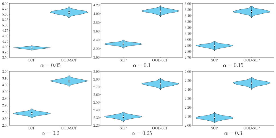
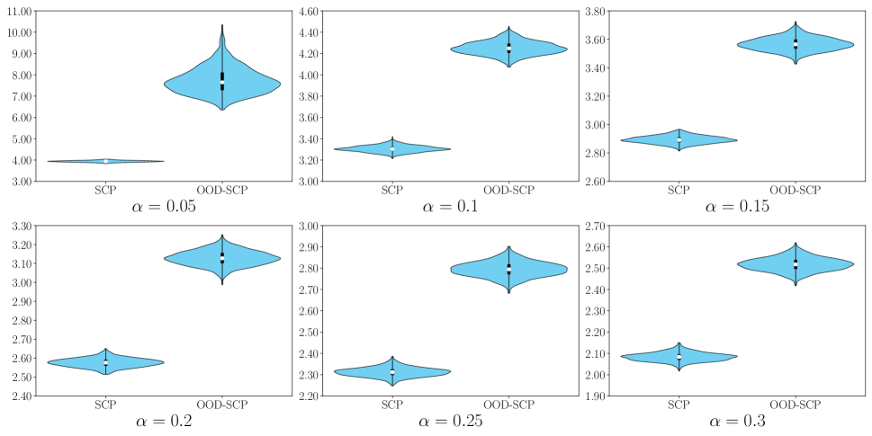
Appendix B B Additional experimental results
In this section, we provide additional experimental results. We provide the results of the average length of the predicted confidence sets in Figures B.1 and B.2, corresponding to the results of the coverage in Figures 2 and 3, respectively.