Forecasting Long-Time Dynamics in Quantum Many-Body Systems by Dynamic Mode Decomposition

Abstract

Numerically computing physical quantities of time-evolved states in quantum many-body systems is a challenging task in general. Here, we propose a method that utilizes reliable short-time data of physical quantities to accurately forecast long-time behavior. The method is based on the dynamic mode decomposition (DMD), which is commonly used in fluid dynamics. The effectiveness and applicability of the DMD in quantum many-body systems such as the Ising model in the transverse field at the critical point are studied, even when the input data exhibits complicated features such as multiple oscillatory components and a power-law decay with long-ranged quantum entanglements unlike fluid dynamics. It is demonstrated that the present method enables accurate forecasts at time as long as nearly an order of magnitude longer than that of the short-time training data. Effects of noise on the accuracy of the forecast are also investigated, because they are important especially when dealing with the experimental data. We find that a few percent of noise does not affect the prediction accuracy destructively.

I Introduction

Recent experimental developments have led to the evolution of diverse measurement techniques, facilitating the detection of novel quantum states and quantum phase transitions in the nonequilibrium dynamics of quantum many-body systems including quantum critical fluctuations characteristic of long-ranged quantum-mechanically entangled systems with strong correlation effects. For instance, in cuprate superconductors, time-dependent optical properties have been investigated by pump-probe measurements employing short-pulse lasers and reported enhanced coherent transport reminiscent of the superconductivity far above the superconducting transition temperature in the equilibrium [1, 2]. In ultracold atomic gases confined in optical lattices that serve as analog quantum simulators on various lattice systems in arbitrary spatial dimensions, quantum gas microscopes [3] or time-of-flight measurements [4] allow for the observation of the time evolution of equal-time correlation functions in quantum many-body systems.

The validation and prediction of experimental results rely on comparing them with outcomes obtained from numerical simulations. Despite the experimental progress in observing time-dependent physical quantities, numerical simulations of the dynamics in quantum many-body systems are still challenging. For example, although obtaining the time-evolved states for systems in one spatial dimension is fairly efficient using the tensor-network methods [5], calculating their dynamics by the tensor-network methods are much harder for systems in two or more spatial dimensions because of highly entangled structures of quantum states after long-time evolution [6, 7, 8, 9, 10, 11, 12]. On the other hand, the time-dependent variational Monte Carlo method [13, 14, 15] with neural-network quantum states [16, 17] is a promising candidate for calculating the dynamics and would be able to simulate the dynamics for a much longer time [18, 19]. However, it often suffers from a high computational cost because of a large number of variational parameters and the requirement for sophisticated optimization of wave functions at each time step.

It would be advantageous to have a method that leverages short-time data of physical quantities to reliably predict long-time behavior. As for forecasting physical quantities after time evolution, it is desired to develop a method that can predict long-time behavior from precise short-time data obtained by experiments or numerical simulations without knowing the time-evolved quantum state itself. There has been a growing interest in predicting the dynamics of observables in quantum many-body systems using machine learning and related techniques [20, 21, 22, 23, 24, 25].

To this end, we focus on the dynamic mode decomposition (DMD), which is commonly used in the field of fluid dynamics [26, 27, 28, 29, 30, 31, 32]. This method is essentially equivalent to the matrix pencil method [33], which was introduced much earlier than the DMD and has been used for estimating frequencies and damping factors of sinusoidal signals from noisy time-series data [34, 35, 36]. The DMD offers advantages in its simplicity of execution and its minimal dependency on assumptions for the system. The computational cost when one uses this algorithm is primarily determined by the expense of performing a singular value decomposition (SVD) of a certain matrix constructed from the short-time data, making it a cost-effective method. The DMD has been applied to the dynamics of quantum systems [37, 38, 39, 40, 41, 42, 43, 44, 45, 46] and the quantum algorithm for dynamic simulations [47, 48, 49, 50, 51] recently. In Refs. [40, 41, 43, 46], the DMD was successful in obtaining nonequilibrium long-time evolution containing many-body effects within the perturbative self-energy. However, whether the DMD offers a useful and efficient tool of an accurate quantum many-body solver for long-time predictions in cases of strongly correlated systems and/or systems with critical fluctuations accompanied by strong quantum entanglement still remain a big challenge.

In this paper, we specifically focus on one of the most challenging problems in the DMD, i.e., the prediction of the long-time dynamics from the short-time reliable data that exhibits multiple oscillatory components and a power-law decay, which stem from the quantum many-body effects. Such behavior already appears in the textbook example of the time-dependent correlation functions in the low-dimensional transverse-field Ising models [52, 53, 54, 55]. We demonstrate that the DMD makes it possible to predict the behavior at time as long as nearly one order of magnitude longer than the range of utilized short-time training data even when the input data exhibits such complicated features by taking the transverse-field Ising models as model systems.

This paper is organized as follows. In Sec. II, we introduce the DMD and describe the details of how one can apply it to the dynamics of the quantum many-body systems. In Sec. III, we demonstrate the effectiveness of the DMD in predicting the time-dependent correlations with oscillatory components. We also examine to what extent the DMD deals with the challenging critical phenomena that exhibits a power-law decay as a function of time and converges to a nonzero value in the infinite-time limit. Moreover, to cope with more practical problems, we show that the present DMD withstands up to a moderate level of noise in the input data and sustains the accuracy. Last but not least, we estimate the systematic and statistical errors of the DMD predictions. In Sec. IV, we draw our conclusions and look to further applications of the DMD in quantum many-body systems.

II Dynamic mode decomposition

We briefly review how one can apply the DMD to a given time-series data [30, 31]. We consider a time-dependent physical quantity $f_{n}=f(n\cdot\Delta t)=f(t)$ that is measured or calculated at discrete time steps $n=0,1,2,\dots,N-1$. Here we assume that the time interval between two consecutive time steps is constant and denote the time interval by $\Delta t$. We would like to predict the time-dependent physical quantity $f_{n}$ for $n=N,N+1,\dots,N_{\rm max}-1$, where $N_{\rm max}-1$ is the maximum number of time steps to be predicted.

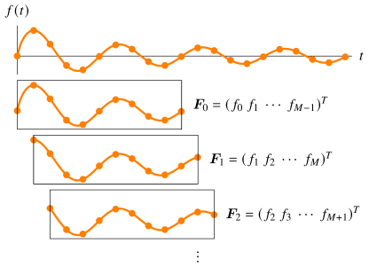
Figure 1: Schematic picture of time-series data of a physical quantity $f_{n}=f(n\cdot\Delta t)=f(t)$ ($n=0,1,2,\dots,N-1$). We separate the time-series data into several short-interval sequences and construct $N-M+1$ vectors. Each column vector contains $M$ elements.

We separate the time-series data into several short-interval sequences as shown in Fig. 1. We construct $N-M+1$ vectors $\bm{F}_{0}$, $\bm{F}_{1}$, …, $\bm{F}_{N-M}$ from the short-interval sequences. Each column vector $\bm{F}_{n}=(f_{n}~{}f_{n+1}~{}\cdots~{}f_{n+M-1})^{T}$ contains $M$ elements. Hereafter, we call each short-interval sequence (column vector) $\bm{F}_{n}$ a snapshot, following the convention [30, 31], although $\bm{F}_{n}$ contains the information of different time from $n$ to $n+M-1$. We then construct two $M\times(N-M)$ matrices $X_{0}$ and $X_{1}$ as

$$X_{0} =\begin{pmatrix}\vline&\vline&\vline&&\vline\\ \bm{F}_{0}&\bm{F}_{1}&\bm{F}_{2}&\cdots&\bm{F}_{N-M-1}\\ \vline&\vline&\vline&&\vline\\ \end{pmatrix}$$ (1)

$$=\begin{pmatrix}f_{0}&f_{1}&f_{2}&\cdots&f_{N-M-1}\\ f_{1}&f_{2}&f_{3}&\cdots&f_{N-M}\\ f_{2}&f_{3}&f_{4}&\cdots&f_{N-M+1}\\ \vdots&\vdots&\vdots&\ddots&\vdots\\ f_{M-1}&f_{M}&f_{M+1}&\cdots&f_{N-2}\\ \end{pmatrix},$$ (2)

$$X_{1} =\begin{pmatrix}\vline&\vline&\vline&&\vline\\ \bm{F}_{1}&\bm{F}_{2}&\bm{F}_{3}&\cdots&\bm{F}_{N-M}\\ \vline&\vline&\vline&&\vline\\ \end{pmatrix}$$ (3)

$$=\begin{pmatrix}f_{1}&f_{2}&f_{3}&\cdots&f_{N-M}\\ f_{2}&f_{3}&f_{4}&\cdots&f_{N-M+1}\\ f_{3}&f_{4}&f_{5}&\cdots&f_{N-M+2}\\ \vdots&\vdots&\vdots&\ddots&\vdots\\ f_{M}&f_{M+1}&f_{M+2}&\cdots&f_{N-1}\\ \end{pmatrix}.$$ (4)

The DMD computes the leading eigendecomposition of the linear operator $A$ that satisfies $X_{1}=AX_{0}$. The $M\times M$ matrix $A$ is given by

$$A=X_{1}X_{0}^{-1},$$ (5)

where $X_{0}^{-1}$ is the Moore-Penrose pseudoinverse of $X_{0}$. Note that $X_{0}^{-1}=X_{0}^{\dagger}(X_{0}X_{0}^{\dagger})^{-1}$ when the number of rows is smaller than that of columns, whereas $X_{0}^{-1}=(X_{0}^{\dagger}X_{0})^{-1}X_{0}^{\dagger}$ otherwise. We can predict the time-series data $\bm{F}_{n}$ for $n=N,N+1,\dots,N_{\rm max}-1$ by sequentially multiplying the matrix $A$ to the vector $\bm{F}_{0}$, i.e., $\bm{F}_{n}\approx A^{n}\bm{F}_{0}$.

When the dimension $M$ of the matrix $A$ is large, the computation of the eigendecomposition of $A$ becomes expensive. Moreover, the matrix $A$ may contain eigenvectors that cause numerical instability. In such cases, we can reduce the computational cost and improve the numerical stability by the truncated SVD. Here we describe how to utilize the truncated SVD to perform the DMD. Hereafter, for simplicity, we assume that the matrix $A$ and that in the reduced subspace (the matrix $\tilde{A}$) are diagonalizable. When the matrix is not diagonalizable, one can modify the following arguments using the Jordan normal form of each matrix [50].

1. We compute the SVD of the matrix $X_{0}$ as

   $$X_{0}=U\Sigma V^{\dagger},$$ (6)

   where $U$ is an $M\times M$ unitary matrix, $V^{\dagger}$ is an $(N-M)\times(N-M)$ unitary matrix, and $\Sigma$ is an $M\times(N-M)$ matrix with only the first $\min(M,N-M)$ diagonal elements being nonzero. The diagonal elements of $\Sigma$ are denoted by $\sigma_{0}\geq\sigma_{1}\geq\cdots\geq\sigma_{\min(M,N-M)-1}\geq 0$. We keep only the first $R$ columns of $U$ and $V$ and the first $R\times R$ submatrix of $\Sigma$. Here $R$ is the rank of the reduced SVD approximation to $X_{0}$ and is determined by the smallest integer that satisfies $\sigma_{R}/\sigma_{0}<\epsilon$ with $\epsilon$ being a cutoff. As a result, we obtain an $M\times R$ matrix $U_{R}$, an $R\times R$ diagonal matrix $\Sigma_{R}$, and an $R\times(N-M)$ matrix $V_{R}^{\dagger}$, respectively. They satisfy

   $$X_{0}\approx U_{R}\Sigma_{R}V_{R}^{\dagger}.$$ (7)

2. We compute the matrix $\tilde{A}$, which is the $R\times R$ projection of $A$, as

   $$\tilde{A}=U_{R}^{\dagger}X_{1}V_{R}\Sigma_{R}^{-1}.$$ (8)

   Here we use the fact that $\tilde{A}\approx U_{R}^{\dagger}AU_{R}$, $A=X_{1}X_{0}^{-1}\approx X_{1}V_{R}\Sigma_{R}^{-1}U_{R}^{\dagger}$, and $U_{R}^{\dagger}U_{R}\approx 1_{R}$, where $1_{R}$ is an $R\times R$ identity matrix.

3. We diagonalize the matrix $\tilde{A}$ as

   $$\tilde{A}W=W\Lambda,$$ (9)

   where $\Lambda={\rm diag}(\lambda_{0},\lambda_{1},\dots,\lambda_{R-1})$ is a diagonal matrix and $W$ is an $R\times R$ unitary matrix.

4. We reconstruct the eigendecomposition of $A$ from $W$ and $\Lambda$ approximately. The approximate dominant $R$ eigenvalues of $A$ are given by $\Lambda$, and the corresponding $R$ eigenvectors of $A$ are given by columns of the $M\times R$ matrix $\Phi$, which is defined by

   $$\Phi=X_{1}V_{R}\Sigma_{R}^{-1}W.$$ (10)

   Indeed, from Eq. (8) and Eq. (9), one can see that

   $$\qquad A\Phi \approx U_{R}\tilde{A}U_{R}^{\dagger}\Phi=U_{R}\tilde{A}U_{R}^{\dagger}X_{1}V_{R}\Sigma_{R}^{-1}W$$

   $$=U_{R}\tilde{A}\tilde{A}W=U_{R}\tilde{A}W\Lambda$$

   $$=U_{R}U_{R}^{\dagger}X_{1}V_{R}\Sigma_{R}^{-1}W\Lambda=U_{R}U_{R}^{\dagger}\Phi\Lambda\approx\Phi\Lambda$$ (11)

   holds.

5. We predict the time-series data $f_{n}=f(n\cdot\Delta t)=f(t)$ for $n=N,N+1,\dots,N_{\rm max}-1$ from $\Phi$ and $\Lambda$. From $\bm{F}_{n}\approx A^{n}\Phi\Phi^{-1}\bm{F}_{0}\approx\Phi\Lambda^{n}\Phi^{-1}\bm{F}_{0}$ with $\Phi^{-1}=\Phi^{-1}$ being the pseudoinverse of $\Phi$, the time evolution of the time-series data is approximately given by

   $$\bm{F}_{n}\approx\Phi\Lambda^{n}\bm{b}=\sum_{k=0}^{R-1}\bm{\phi}_{k}(\lambda_{k})^{n}b_{k}.$$ (12)

   Here the $M$ component vector $\bm{\phi}_{k}$ is the $k$th column of $\Phi$, and the vector $\bm{b}=(b_{0}~{}b_{1}~{}\cdots~{}b_{R-1})^{T}$ is determined by the initial vector $\bm{F}_{0}$ and the pseudoinverse of $\Phi$ as

   $$\bm{b}=\Phi^{-1}\bm{F}_{0}.$$ (13)

The computational cost of the DMD is dominated by the computation of the truncated SVD of $X_{0}$. When the upper bound $R^{\rm upper}$ for the rank of the truncated SVD is given in advance, i.e., $R\leq R^{\rm upper}$ and $R^{\rm upper}\ll M,(N-M)$, the computational cost of the DMD becomes ${\cal O}[M(N-M)R^{\rm upper}]$. The cost can be further reduced by applying the randomized SVD [56] and is given by ${\cal O}[M(N-M)\log R^{\rm upper}]$. This cost is much cheaper than the computational cost ${\cal O}(M^{3})$ of the direct eigendecomposition of $A$ when $M\sim(N-M)$.

III Application to the quantum dynamics

We apply the DMD to the dynamics of quantum many-body systems and discuss the accuracy and applicability of the DMD. We specifically consider the following cases: (i) correlation functions that exhibit multiple oscillatory modes and (ii) correlation functions that exhibit oscillatory behavior and have a power-law decay. In case (i), we choose the two-dimensional (2D) transverse-field Ising model as a model system. For a small finite system, the time evolution of equal-time spin-spin correlation functions after a sudden quench exhibit oscillatory behavior without damping. In case (ii), we choose the one-dimensional (1D) transverse-field Ising model at the critical point as a model system, where a strong long-range quantum entanglement is expected providing us with a challenge in conventional numerical simulations [57]. For a sufficiently large system, the unequal-time (time-displaced) spin-spin correlation functions exhibit oscillatory behavior with a power-law decay on top of the convergence to a nonzero value in the infinite-time limit. We show that the DMD can predict the time evolution of the correlation functions in both cases with high accuracy. Moreover, we discuss the error analysis of the DMD.

III.1 Time-dependent correlation functions without damping

We focus on the transverse-field Ising model

$$H=-J\sum_{\langle i,j\rangle}S^{z}_{i}S^{z}_{j}-\Gamma\sum_{i}S^{x}_{i},$$ (14)

under the periodic boundary condition, where $S_{i}^{\alpha}$ ($\alpha=x,y,z$) are the $S=1/2$ Pauli spins, $J$ is the strength of the nearest-neighbor interaction, and $\Gamma$ is the strength of the transverse magnetic field. The symbol $\langle\cdots\rangle$ denotes nearest-neighbor site pairs. Hereafter, we set the lattice constant $a$ and the Planck $\hbar$ constant to unity. We take the units of energy and time as $J$ and $J^{-1}$, respectively, unless otherwise noted.

We obtain the time evolution of the equal-time longitudinal spin-spin correlation functions in the following manner. We consider the model in Eq. (14) on a square lattice with a system size $N_{\mathrm{s}}=L^{2}$ for $L=4$. We first prepare the initial state as

$$|\psi_{0}\rangle=\bigotimes_{i=1}^{N_{\mathrm{s}}}\frac{|\uparrow\rangle_{i}+|\downarrow\rangle_{i}}{\sqrt{2}},$$ (15)

which is the ground state of the transverse-field Ising model at $\Gamma/J=\infty$. We then perform a sudden quench by changing the transverse magnetic field from $\Gamma/J=\infty$ to the critical point $\Gamma/J=\Gamma_{\rm c}^{\rm 2D}/J\approx 1.522$ [58, 59, 60]. The time evolution of equal-time longitudinal spin-spin correlation functions at distance $\bm{r}$ and time $t$ are given by

$$C^{zz}_{\rm eq}(\bm{r},t)=\langle\psi_{0}|S^{z}_{\bm{0}}(t)S^{z}_{\bm{r}}(t)|\psi_{0}\rangle\,,$$ (16)

with $S^{z}_{\bm{r}}(t)=e^{iHt}S^{z}_{\bm{r}}e^{-iHt}$. As for a small finite system, we can use the exact diagonalization method to calculate the equal-time correlation functions over arbitrarily long periods. We calculate the correlation functions for $t\in[0,1000)$ with a time step $\Delta t=0.05$ and $N_{\rm max}=20000$ using the QuSpin library [61, 62].

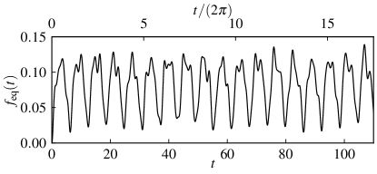
Figure 2: Exact time evolution of the equal-time longitudinal spin-spin correlation function after a sudden quench in the 2D transverse-field Ising model on a finite-size square lattice ($4\times 4$ sites).

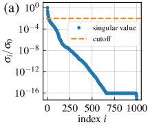
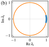
Figure 3: DMD parameters in the case of the equal-time longitudinal spin-spin correlation function after a sudden quench in the 2D transverse-field Ising model on a square lattice. (a) Singular values $\sigma_{i}$ of the truncated SVD of the matrix $X_{0}$. (b) Eigenvalues $\lambda_{i}$ of the matrix $\tilde{A}$.

We show the exact time evolution of the correlation function at distance $|\bm{r}|=1$, i.e.,

$$f_{\rm eq}(t)=C^{zz}_{\rm eq}(|\bm{r}|=1,t)$$ (17)

in Fig. 2. Although the 2D transverse-field Ising model is nonintegrable, and thus the thermalization would occur and the correlation function would converge to a nearly constant value after a long time in the thermodynamic limit, the correlation function does not exhibit damping in a small finite system. The correlation function exhibits oscillatory behavior, and the period of the dominant oscillation is found to be $T\approx 2\pi/J$.

For the DMD, we choose $M=1000$ and $N=2M$, which correspond to the time length of the short-interval sequence $t_{\rm snap}=M\cdot\Delta t=50$ and the whole time interval of input data $t_{\rm input}=N\cdot\Delta t=100$, respectively. The calculated singular values $\sigma_{i}$ decay exponentially as a function of the index $i$, with a steep exponent at small index $i\leq 13$ and milder exponents at larger index $i$ as shown in Fig. 3(a). We should choose a sufficiently small cutoff $\epsilon$ to include relevant modes of the dynamics as many as possible; at the same time, we also need a reasonably not too-small cutoff $\epsilon$ to avoid the inclusion of irrelevant modes that cause the divergence of time series for long $t$. In the case of the present model, we numerically find that the DMD prediction becomes unstable when the cutoff $\epsilon$ is smaller than $0.01$. Therefore, the cutoff is chosen to be $\epsilon=0.01$, and the rank $R$ of the truncated SVD becomes only $R=13$. The absolute values of the calculated eigenvalues $|\lambda_{i}|$ of the matrix $\tilde{A}$ are smaller than or equal to unity [see Fig. 3(b)], indicating that the dynamics obtained by the DMD is stable.

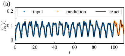
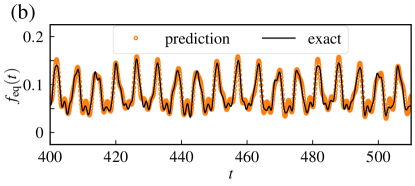
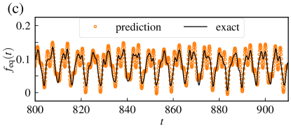
Figure 4: DMD prediction of the equal-time longitudinal spin-spin correlation function in the 2D transverse-field Ising model. We show the time evolution of the correlation function for (a) $t\in[0,110]$, (b) $t\in[400,510]$, and (c) $t\in[800,910]$. The solid line is the exact result, the filled blue circles are the input data, and the open orange circles are the predicted data. The data points $f_{{\rm eq},n}=f_{\rm eq}(n\cdot\Delta t)=f_{\rm eq}(t)$ are plotted only when $n$ is an even number.

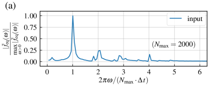
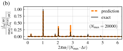
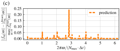
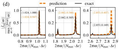
Figure 5: Fourier transform of the equal-time longitudinal spin-spin correlation function in the 2D transverse-field Ising model. We remove a large value at $\omega=0$. (a) Exact result when $t\in[0,100)$ ($N_{\rm max}=2000$). (b) Comparison of the exact result (solid line) and the DMD prediction (dashed line) for the absolute value of the Fourier-transformed correlation function when $t\in[0,1000)$ ($N_{\rm max}=20000$). (c) Relative difference between the exact result and the DMD prediction. (d) Magnified views of Fig. 5(b). The position and intensity of each peak are also shown in the figure in the order (position, intensity). All the positions of the peaks of the DMD prediction coincide with those of the exact result.

We show the selected time evolution of the predicted correlation function for $t\in[0,110]$, $t\in[400,510]$, and $t\in[800,910]$ in Figs. 4(a-c). For $t\lesssim 500$, the DMD prediction (open circles) and the exact result (solid line) are in good agreement. In this sense, the DMD can predict the time evolution of the correlation function with high accuracy up to approximately five times the duration of the input time. As the time $t$ increases, the DMD prediction deviates from the exact result. Indeed, for $t\in[800,910]$, we observe that the amplitude of the oscillation in the DMD prediction is slightly larger than that in the exact result. On the other hand, the overall structure of the DMD prediction remains similar to that of the exact result even at $t\geq 800$, namely at an order of magnitude longer time than $t_{\rm input}$.

We also show the Fourier transform of the predicted correlation function, which is defined by

$$\tilde{f}(\omega)=\sum_{n=0}^{N_{\rm max}-1}f_{n}\exp\left(-\frac{2\pi i\omega n}{N_{\rm max}}\right)$$ (18)

for $\omega=0,1,\dots,N_{\rm max}-1$ in Fig. 5. We remove a relatively larger component at $\omega=0$ hereafter. As a reference, we plot the exact result when $t\in[0,100)$ ($N_{\rm max}=2000$) in Fig. 5(a). We will examine how the DMD prediction reproduces the exact result for $t\in[0,1000)$ ($N_{\rm max}=20000$) when using this reference as input data. Note that the prediction based on the Gaussian process regression (GPR) method [63, 64], which is a conventional machine learning method, fails to reproduce the exact peak positions as shown in Appendix A.

As shown in Fig. 5(b), the DMD prediction (dashed bold line) of the absolute value of the Fourier-transformed correlation function is in good agreement with the exact result (thin solid line) for all the frequencies $\omega$. When the data is normalized by $\max_{\omega>0}|\tilde{f}^{\rm exact}(\omega)|$ for all frequencies $\omega$, the relative difference between the exact result and the DMD prediction is at most $25\%$ and is nearly less than $5\%$ for most of the frequencies $\omega$ as shown in Fig. 5(c). Although the difference becomes larger for peaks with smaller exact intensities as shown in Fig. 5(d), the peak positions are exactly reproduced when the peak intensity is larger than $10\%$ of the maximum value of the exact $\tilde{f}(\omega)$ (see Appendix B for more detailed comparisons). In this sense, the DMD is a more powerful method than the GPR method at least in the prediction of the time evolution.

III.2 Time-dependent Correlation functions with a power-law decay

Next, we focus on a more challenging case where the correlation functions exhibit oscillatory behavior with a power-law decay arising from the long-distance long-time quantum entanglement at a critical point of phase transition [57]. We consider the transverse-field Ising model in Eq. (14) on a chain with an infinite system size. We prepare the initial state $|\psi_{0}^{\prime}\rangle$ as the ground state of the transverse-field Ising model at the critical point $\Gamma/J=\Gamma_{\rm c}^{\rm 1D}/J=0.5$ [65]. The transverse unequal-time (time displaced) spin-spin correlation functions at distance $r$ and time displacement $t$ are defined by

$$C^{xx}_{\rm uneq}(r,t)=\langle\psi_{0}^{\prime}|S^{x}_{0}(0)S^{x}_{r}(t)|\psi_{0}^{\prime}\rangle$$ (19)

with $S^{x}_{r}(t)=e^{iHt}S^{x}_{r}e^{-iHt}$. The 1D transverse-field Ising model is integrable. The exact correlation functions can be calculated after the Jordan-Wigner transformation from spin operators to fermion operators [66] and, at $\Gamma=\Gamma_{\rm c}^{\rm 1D}$, they are given by

$$C^{xx}_{\rm uneq}(r,t) =\frac{1}{\pi^{2}}+\frac{1}{4}\left[J_{2r}(2\Gamma t)+iE_{2r}(2\Gamma t)\right]^{2}$$

$$~{}\phantom{=}~{}-\frac{1}{4}\left[J_{2r-1}(2\Gamma t)+iE_{2r-1}(2\Gamma t)\right]$$

$$~{}\phantom{==}~{}\times\left[J_{2r+1}(2\Gamma t)+iE_{2r+1}(2\Gamma t)\right],$$ (20)

where

$$J_{r}(x)=\frac{1}{\pi}\int_{0}^{\pi}\cos(r\theta-x\sin\theta)\,d\theta$$ (21)

is the Bessel function of $r$th order and

$$E_{r}(x)=\frac{1}{\pi}\int_{0}^{\pi}\sin(r\theta-x\sin\theta)\,d\theta$$ (22)

is the related Anger-Weber or Lommel-Weber function [52, 53].

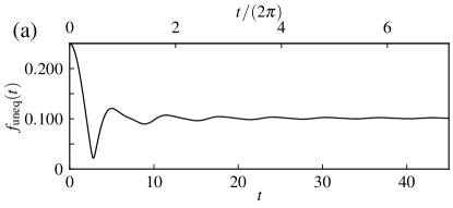
Figure 6: Exact time evolution of the absolute value of the unequal-time onsite transverse spin-spin correlation function in the 1D transverse-field Ising model on an infinite chain.

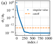
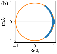
Figure 7: DMD parameters in the case of the unequal-time onsite transverse spin-spin correlation function for the 1D transverse-field Ising model on an infinite chain. (a) Singular values $\sigma_{i}$ of the truncated SVD of the matrix $X_{0}$. (b) Eigenvalues $\lambda_{i}$ of the matrix $\tilde{A}$.

We show the exact time evolution of the absolute value of the unequal-time onsite ($r=0$) correlation function, i.e.,

$$f_{\rm uneq}(t)=|C^{xx}_{\rm uneq}(r=0,t)|$$ (23)

in Fig. 6. The correlation function exhibits oscillatory behavior with a power-law decay [53, 54, 55] and converges to a nonzero value corresponding to the squared transverse magnetization $m_{x}^{2}=1/\pi^{2}$ at $\Gamma=\Gamma_{\rm c}^{\rm 1D}$ in the infinite-time limit [55]. The long-time asymptotic envelope function is scaled as

$$\left|\,\left|C^{xx}_{\rm uneq}(r=0,t)\right|-m_{x}^{2}\right|\sim t^{-3/2}$$ (24)

for $t\gg 1$ [53]. The period of the dominant oscillation is $T\approx\pi/\Gamma=2\pi/J$.

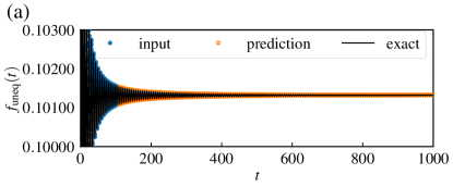
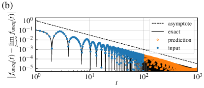
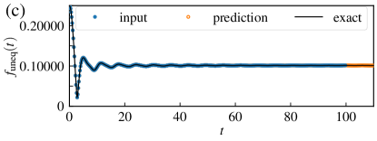
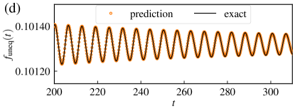
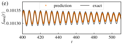
Figure 8: DMD prediction of the unequal-time onsite transverse spin-spin correlation function in the 1D transverse-field Ising model. We show the time evolution of the absolute value of the correlation function for (a) $t\in[0,1000)$ and (b) that in the logarithmic scale. The magnified views of the time evolution for (c) $t\in[0,110]$, (d) $t\in[200,310]$, and (e) $t\in[400,510]$ are also shown. The solid line is the exact result, the filled circles are the input data, and the open circles are the predicted data. The data points $f_{{\rm uneq},n}=f_{\rm uneq}(n\cdot\Delta t)=f_{\rm uneq}(t)$ are plotted only when $n$ is a multiple of $20$.

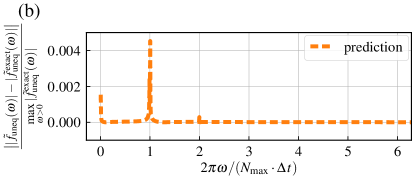
Figure 9: Fourier transform of the unequal-time onsite transverse spin-spin correlation function in the 1D transverse-field Ising model. We remove a divergently large value at $\omega=0$. (a) Comparison of the exact result (solid line) and the DMD prediction (dashed line) for the absolute value of the Fourier-transformed correlation function. (b) Relative difference between the exact result and the DMD prediction.

For the DMD, we choose $\Delta t=0.01$, $M=5000$, $N=2M$, and $N_{\rm max}=100000$. The calculated singular values $\sigma_{i}$ decay exponentially as a function of the index $i$, as shown in Fig. 7(a). In the case of the 1D transverse-field Ising model, we numerically find that the DMD prediction is rather stable even when the cutoff $\epsilon$ is smaller than $0.01$, which is the value for the 2D transverse-field Ising case. This observation suggests that the number of relevant eigenmodes in the case with damping is larger than that in the case without damping, and many eigenmodes are responsible for the dynamics exhibiting a power-law decay. Therefore, the cutoff is chosen to be a very small value $\epsilon=5\times 10^{-14}$, and the rank $R$ of the truncated SVD becomes $R=193$. Even with such a small cutoff, the absolute values of the calculated eigenvalues $|\lambda_{i}|$ of the matrix $\tilde{A}$ are smaller than unity [see Fig. 7(b)], indicating that the dynamics obtained by the DMD is stable.

We show the time evolution of the predicted correlation function for $t\in[0,1000)$ in Fig. 8(a) and that in the logarithmic scale in Fig. 8(b). The predicted correlation function (open circles) appears to converge to a nonzero value in the very long-time limit, which is consistent with the exact result (solid line). We also show the magnified time evolution of the predicted correlation function for $t\in[0,110]$, $t\in[200,310]$, and $t\in[400,510]$ in Figs. 8(c-e). For $t\lesssim 400$, the DMD prediction and the exact result agree very well. The period of the dominant oscillation and the convergent value in the infinite-time limit are well reproduced by the DMD prediction. On the other hand, for $t\gtrsim 400$, the amplitude of the oscillation in the DMD prediction is slightly smaller than that in the exact result. The deviation gets slightly larger as the time $t$ increases, although the period and center of the oscillation are still well reproduced by the DMD prediction. We also examine the asymptotic behavior of the predicted correlation function [see the logarithmic plot in Fig. 8(b)]. For $t\lesssim 700$, The DMD prediction decays as a power law with the exponent close to $-3/2$, which is the same as the exact result. When the eigenmodes are sufficiently included in the DMD procedure, the DMD prediction nicely reproduces the exact result for a very long time, which is more than five times the duration of the input time $t_{\rm input}$.

Note that the DMD prediction gets slightly better when the origin of the time series is shifted to later times. This is because we can neglect the initial transient behavior that does not follow the power-law decay in a strict sense. The effect of the shift of the origin of the time series will be discussed in Appendix C.

The comparison of the Fourier transform of the predicted correlation function and the exact result is shown in Fig. 9(a). Because the $\omega=0$ component of the Fourier transform is divergently large, we remove the value at $\omega=0$. The relative difference between the exact result and the DMD prediction is less than $0.4\%$ over all frequencies [see Fig. 9(b)].

III.3 Effects of noise

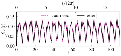
Figure 10: Time evolution of the equal-time longitudinal spin-spin correlation function after a sudden quench in the 2D transverse-field Ising model on a finite-size square lattice with additive white Gaussian noise (dashed pink line). As a reference, the time evolution without noise is also shown (solid black line).

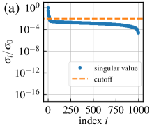
Figure 11: DMD parameters in the case of the equal-time longitudinal spin-spin correlation function after a sudden quench in the 2D transverse-field Ising model on a square lattice with additive white Gaussian noise. (a) Singular values $\sigma_{i}$ of the truncated SVD of the matrix $X_{0}$. Singular values with $\sigma_{i}/\sigma_{0}\lesssim 10^{-3}$ as a function of index $i$ exhibit wide plateau-like behavior. The cutoff is chosen to be larger than the value at the plateau. (b) Eigenvalues $\lambda_{i}$ of the matrix $\tilde{A}$.

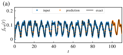
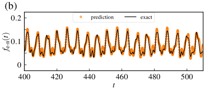
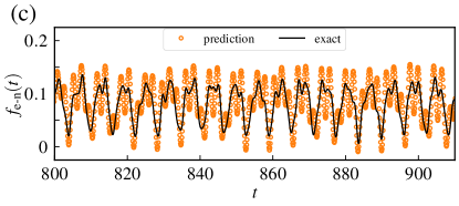
Figure 12: DMD prediction of the equal-time longitudinal spin-spin correlation function in the 2D transverse-field Ising model with additive white Gaussian noise. We show the time evolution of the correlation function for (a) $t\in[0,110]$, (b) $t\in[400,510]$, and (c) $t\in[800,910]$. The solid line is the exact result, the filled blue circles are the input data, and the open orange circles are the predicted data. The data points $f_{{\rm e\text{-}n},n}=f_{\rm e\text{-}n}(n\cdot\Delta t)=f_{\rm e\text{-}n}(t)$ are plotted only when $n$ is an even number.

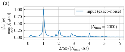
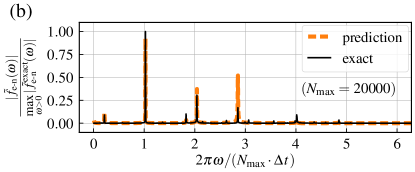
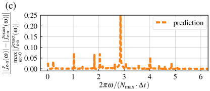
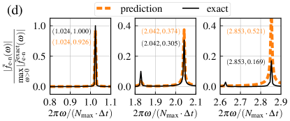
Figure 13: Fourier transform of the equal-time longitudinal spin-spin correlation function in the 2D transverse-field Ising model with additive white Gaussian noise. We remove a large value at $\omega=0$. (a) Exact result when $t\in[0,100)$ ($N_{\rm max}=2000$). (b) Comparison of the exact result (solid line) and the DMD prediction (dashed line) for the absolute value of the Fourier-transformed correlation function when $t\in[0,1000)$ ($N_{\rm max}=20000$). (c) Relative difference between the exact result and the DMD prediction. (d) Magnified views of Fig. 13(b). The position and intensity of each peak are also shown in the figure in the order (position, intensity). All the positions of the peaks of the DMD prediction coincide with those of the exact result.

We investigate how noise in input data affects the prediction by the DMD method. In experiments, time-series data are always affected by noise. In numerical simulations based on the Monte Carlo method, we often need to average over many samples to obtain the time-series data; consequently, the data inevitably have statistical errors. Therefore, examination of the effects of noise is important for practical applications of the DMD method.

In this section, we consider time-series data $f_{\rm n}(t)$ affected by noise $\eta(t)$, which is given by Gaussian white random variables, namely, Gaussian noise with zero mean and variance $\sigma_{\rm noise}^{2}$ without correlations between different time steps. We will demonstrate that the DMD method withstands noise when the noise level is moderate and not too high by taking the time-dependent correlation function in the transverse-field Ising model as an example. The standard deviation $\sigma_{\rm noise}$ is assumed to be substantially smaller than the amplitude of original $f_{\rm orig}(t)$ obtained by the evolution without noise and is defined as

$$\sigma_{\rm noise}=\epsilon_{\rm noise}\max_{t\in[0,(N-1)\cdot\Delta t]}|f_{\rm orig}(t)|,$$ (25)

where $\epsilon_{\rm noise}$ is a small positive parameter that characterizes the strength of noise.

For simplicity, as a noiseless time-series data, we choose the time-dependent correlation function without damping of the 2D transverse-field Ising model in Sec. III.1. (See also Appendix D for the effects of noise on the time-dependent correlation function with a power-law decay in Sec. III.2.) Then, the time-series data $f_{\rm e\text{-}n}(t)$ affected by noise $\eta(t)$ is given by

$$f_{\rm e\text{-}n}(t)=C^{zz}_{\rm eq}(|\bm{r}|=1,t)+\eta(t),$$ (26)

where $C^{zz}_{\rm eq}(|\bm{r}|=1,t)$ is defined in Eq. (16). As for this input data, we have numerically confirmed that the prediction up to $N_{\rm max}=20000$ by the DMD method withstands against the noise when $\epsilon_{\rm noise}\lesssim 0.03$. Hereafter, we set $\epsilon_{\rm noise}=0.03$ and compare the differences of the DMD predictions with and without noise. The corresponding input data $f_{\rm e\text{-}n}(t)$ with noise is shown in Fig. 10.

For the DMD, we choose the same parameters as those in Sec. III.1. In the presence of noise, the calculated singular values $\sigma_{i}$ of the matrix $X_{0}$ drops rapidly for a small index $i\lesssim 20$ and exhibit wide plateau-like behavior for a large index $i\gtrsim 20$ [see Fig. 11(a)]. The plateau-like behavior is caused by the noise, and the typical ratio $\sigma_{i}/\sigma_{0}$ at the plateau is found to be proportional to $\epsilon_{\rm noise}$ (see Appendix E). Therefore, even if we do not know the noise level a priori, we can estimate the strength of noise in the input data by finding the position of the plateau in the plot of singular values $\sigma_{i}/\sigma_{0}$ as a function of index $i$.

The cutoff is chosen to be larger than the value at the plateau so that the irrelevant modes below the noise level are excluded. We choose the cutoff $\epsilon=0.01$, which is the same as the parameter in Sec. III.1. With this choice, the rank $R$ of the truncated SVD becomes $R=15$. The predicted long-time dynamics would be stable because the absolute values of the eigenvalues $|\lambda_{i}|$ of the matrix $\tilde{A}$ are smaller than or equal to unity [see Fig. 11(b)].

We show the selected time evolution of the predicted correlation function for $t\in[0,110]$, $t\in[400,510]$, and $t\in[800,910]$ in Figs. 12(a-c). For $t\lesssim 500$, the DMD prediction and the exact result are in good agreement, just as in the case without noise in Fig. 4. For $t\in[800,910]$, the amplitude of the oscillation in the DMD prediction gets larger than that in the exact result. The extent of the deviation from the exact result is also larger than that without noise. On the other hand, the period of the oscillation in the DMD prediction remains the same as that in the exact result. Therefore, we conclude that the DMD prediction reproduces the exact result for a long time, which is still longer than five times the duration of the noisy input data.

We then calculate the Fourier transform of the correlation function in the presence of noise. We examine how the DMD prediction reproduces the exact result when using the input data with noise in Fig. 13(a).

The DMD prediction reproduces the exact result fairly well even in the presence of noise [see Figs. 13(b)]. The dominant peaks in the Fourier spectrum are located at the same positions as those in the exact result. The relative difference is smaller than $10\%$ for most of the frequencies $\omega$. On the other hand, the relative difference between the exact result and the DMD prediction is larger than that without noise [see Fig. 13(c)]. As the intensity of the peaks in the Fourier spectrum increases, the relative difference between the exact result and the DMD prediction becomes smaller [see Fig. 13(d)].

III.4 Error analysis

In general, the prediction of short-time dynamics is more accurate than that of long-time dynamics because the error is accumulated as the time increases. It would be helpful to know the reliability of the DMD prediction as a function of time. In this section, we estimate the error of the DMD prediction by performing the statistical analysis of the predicted data.

For simplicity, we consider a noiseless time-series data and focus on the case without damping, i.e., the equal-time longitudinal spin-spin correlation function after a sudden quench in the transverse-field Ising model on a finite-size square lattice. To reduce the computational cost, we choose a larger time step $\Delta t=0.2$ and a smaller number of points in each snapshot $M=100$. On the other hand, we choose a larger number of snapshots $N=5M$ so that the time interval of the input data $t_{\rm input}=N\cdot\Delta t=100$ is the same as that in Sec. III.1. We numerically find that the DMD prediction is rather stable without introducing the cutoff $\epsilon$.

The DMD prediction contains two types of errors: one is the systematic error and the other is the statistical error. The systematic error is evaluated by the average difference between the DMD prediction and the exact result. On the other hand, the statistical error is characterized by the standard deviation of the DMD prediction when the input data is selected randomly. In the present setup, we can calculate the exact input data of small systems for arbitrarily long times. Therefore, we will estimate both systematic and statistical errors by comparing the DMD prediction with the exact result.

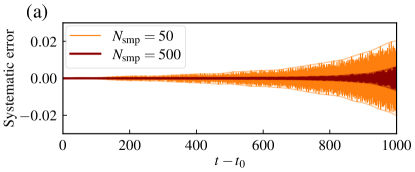
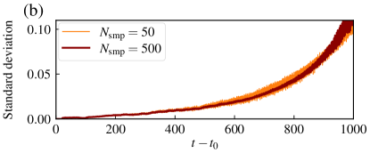
Figure 14: Error analysis of the DMD prediction of the equal-time longitudinal spin-spin correlation function after a sudden quench in the 2D transverse-field Ising model on a square lattice. We show (a) the systematic error and (b) the statistical error of the DMD prediction. The former is obtained by the average of the differences between the DMD predictions and the exact results and the latter is obtained by the standard deviation of the differences for $N_{\rm smp}=50$ and $N_{\rm smp}=500$ samples. The thin lines are the envelope of the systematic error.

To estimate both systematic and statistical errors, we prepare the DMD prediction data by changing the initial time $t_{0}$ of the input data and perform the statistical analysis. We obtain the exact result for the time interval $t\in[0,500000)$ in this section and arrange independent $N_{\rm smp}=500$ samples of the predicted data with different initial times $t_{0}=0,1000,2000,\ldots,499000$ and the maximum time $t_{\rm max}=N_{\rm max}\cdot\Delta t=1000$.

We obtain the systematic error by taking the average of the differences between the DMD predictions and the exact results for $N_{\rm smp}$ samples in the time interval $t-t_{0}\in[0,1000)$ having different initial times $t_{0}$. We also estimate the statistical error from the standard deviation of the differences. Since the initial times $t_{0}$ are sufficiently far apart, the systematic error for different initial times should behave similarly. At a given time-difference point $t-t_{0}$, the statistical error of each sample is expected to follow the same probability distribution.

We show the systematic error of the DMD prediction in Fig. 14(a). The systematic error oscillates around zero, which suggests that the DMD prediction does not have a systematic bias that leads to a deviation of the center of the oscillatory behavior. Indeed, the systematic error is smaller than the statistical error, as we will see below. The systematic error approaches zero as $N_{\rm smp}$ increases. Thus, it is less likely that the DMD prediction has a systematic error. Though the amplitude of the oscillatory systematic error increases as the time difference increases, even at the latest time $t-t_{0}=1000$, it is still smaller than $0.01$ for $N_{\rm smp}=500$, which is less than the amplitude of the spin-spin correlation function.

We also show the statistical error of the DMD prediction in Fig. 14(b). The statistical error monotonically increases as the time difference increases. At $t-t_{0}\approx 800$, the statistical error reaches $0.05$, which is comparable to the amplitude of the spin-spin correlation function. Therefore, the DMD prediction is reliable up to the time scale $t-t_{0}\approx 800$, which is more than five times but slightly less than an order of magnitude as compared to the duration of the input time. As for the present data, the statistical error has more influence on the accuracy of the DMD prediction than the systematic error.

IV Summary and outlook

In conclusion, we have applied the DMD to the dynamics of quantum many-body systems and discussed the accuracy and applicability of the DMD. We have studied the following cases: (i) Correlation functions that exhibit multiple oscillatory components and (ii) correlation functions that exhibit oscillatory behavior and have a power-law decay. The former case is observed in the equal-time longitudinal spin-spin correlation function after a sudden quench in a finite-size system of the 2D transverse-field Ising model, whereas the latter case is realized in the unequal-time transverse spin-spin correlation function in the 1D transverse-field Ising model at the critical point. We have found that the DMD prediction is very accurate when the eigenmodes are sufficiently included in the DMD procedure. The DMD prediction is reliable up to the time scale typically more than five times to nearly an order of magnitude longer than the time interval of the initial input data.

To deal with more realistic situations, we have applied the DMD to noisy input data. We have found that the DMD prediction is still accurate when the noise level is within a few percent of the noiseless part. Moreover, we have empirically found that the singular values of the matrix $X_{0}$ in Eq. (1) generated by the input data exhibit a plateau region when the input data is noisy. The strength of noise is found to be proportional to the plateau value. This observation would be useful for estimating the noise level in experimental or numerical data when the noise level is not known.

We have also estimated the systematic and statistical errors of the DMD prediction. We prepare independent samples of the predicted data with different initial times. Then, the systematic error is obtained by the average of the differences between the DMD predictions and the exact results, whereas the statistical error is obtained by the standard deviation. The statistical error is found to be more influential on the accuracy of the DMD prediction than the systematic error. The statistical error reaches the amplitude of the spin-spin correlation function when the time difference is nearly an order of magnitude longer than the duration of the input time. Extending the time scale of the reliable DMD prediction by more than an order of magnitude longer is important future work.

Our findings open up the possibility of applying the DMD to the dynamics of other quantum many-body systems, which are difficult to simulate by conventional brute-force numerical methods that require calculating time-evolved wave functions. We have shown that the DMD is a powerful and versatile tool even at quantum critical points with temporary long-ranged quantum fluctuations characteristic of the growing quantum entanglement. It is also interesting to apply the DMD to the time series of experimental data in quantum many-body systems. Such an application is expected to be useful and will be discussed in future work.

Appendix A Prediction by the GPR method

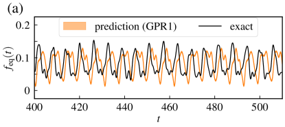
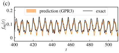
Figure 15: GPR prediction of the equal-time longitudinal spin-spin correlation function in the 2D transverse-field Ising model. We show the time evolution for $t\in[400,510]$. We show the results when the number of periodic kernels is (a) $N_{\rm ker}=1$, (b) $N_{\rm ker}=2$, and (c) $N_{\rm ker}=3$.

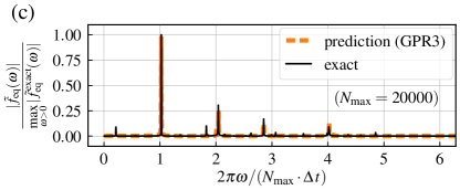
Figure 16: Fourier transform of the GPR prediction of the equal-time longitudinal spin-spin correlation function in the 2D transverse-field Ising model. We remove the value at $\omega=0$. We show the results when the number of periodic kernels is (a) $N_{\rm ker}=1$, (b) $N_{\rm ker}=2$, and (c) $N_{\rm ker}=3$.

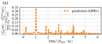
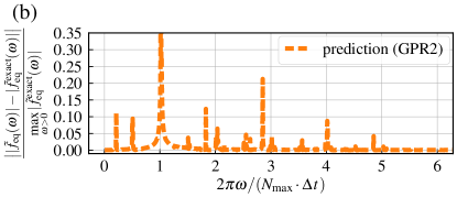
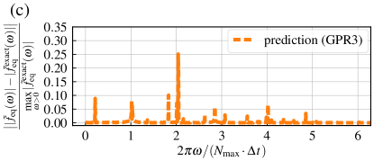
Figure 17: Relative difference between the Fourier transform of the GPR prediction and the exact result in the 2D transverse-field Ising model. We show the results when the number of periodic kernels is (a) $N_{\rm ker}=1$, (b) $N_{\rm ker}=2$, and (c) $N_{\rm ker}=3$.

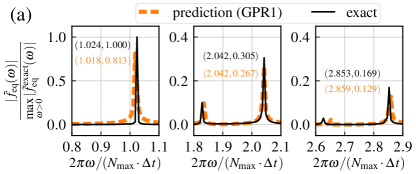
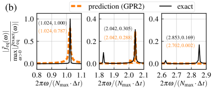
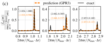
Figure 18: Magnified views of Fig. 16 in the 2D transverse-field Ising model. We show the results when the number of periodic kernels is (a) $N_{\rm ker}=1$, (b) $N_{\rm ker}=2$, and (c) $N_{\rm ker}=3$. The position and intensity of each peak are also shown in the figure in the order (position, intensity).

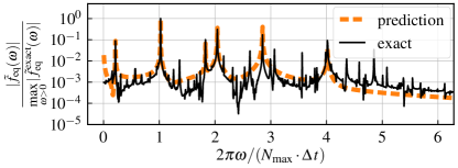
Figure 19: Fourier transform of the equal-time longitudinal spin-spin correlation function in the 2D transverse-field Ising model. We compare the exact result (solid line) and the DMD prediction (dashed line) for the absolute value of the Fourier-transformed correlation function. The vertical axis is in the logarithmic scale.

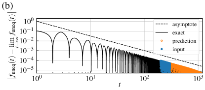
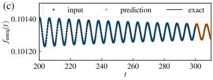
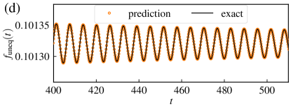
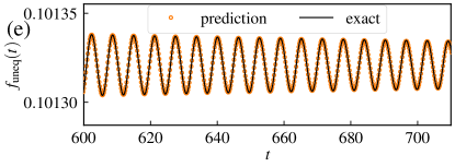
Figure 20: DMD prediction of the unequal-time onsite transverse spin-spin correlation function in the 1D transverse-field Ising model when the origin of the time series is shifted by $t_{\rm 0}=200$. We show the time evolution of the absolute value of the correlation function for (a) $t\in[0,1200)$ and (b) that in the logarithmic scale. The magnified views of the time evolution for (c) $t\in[200,310]$, (d) $t\in[400,510]$, and (e) $t\in[600,710]$ are also shown. The solid line is the exact result, the blue filled circles are the input data, and the orange open circles are the predicted data. The data points $f_{{\rm uneq},n}=f_{\rm uneq}(n\cdot\Delta t)=f_{\rm uneq}(t)$ are plotted only when $n$ is a multiple of $20$.

We examine the accuracy of the GPR method [63, 64] compared to that of the DMD for the example of the equal-time longitudinal spin-spin correlation function after a sudden quench in a finite-size system of the 2D transverse-field Ising model shown in Sec. III.1. The GPR method is a technique used to interpolate function values for unobserved data from input data. It relies on the assumption that for similar input $t$, the corresponding output $f(t)$ will also be similar. Even when linear regression struggles to fit the data adequately, the GPR method is able to find a suitable fit in a number of cases. The GPR method is also useful for estimating the error of the prediction. Moreover, by appropriately selecting the kernel function, we can flexibly choose the model to fit the data.

We choose the kernel functions for the GPR method in the following manner. Because the equal-time longitudinal spin-spin correlation function after a sudden quench exhibits nearly periodic oscillations, we choose the periodic kernel function

$$k_{\rm per}(t,t^{\prime})=\sigma_{\rm per}^{2}\exp\left[-\frac{2\sin^{2}\left(\pi|t-t^{\prime}|/T_{\rm per}\right)}{l_{\rm per}^{2}}\right]$$ (27)

with the variance $\sigma_{\rm per}^{2}$, the period $T_{\rm per}$, and the length scale $l_{\rm per}$. To cope with multiple oscillatory components in the equal-time longitudinal spin-spin correlation function, we study a sum of periodic kernel functions with different variances $\sigma_{\rm per}^{2}$, periods $T_{\rm per}$, and length scales $l_{\rm per}$. Number of periodic kernel functions ($N_{\rm ker}$) is increased to improve the accuracy of the prediction. As for finite-size systems we considered, the correlation function does not show damping. Therefore, we do not introduce additional kernel functions such as the radial basis kernel function, which is often used to model growing or decaying behavior.

For the optimization of the kernel parameters, we take the following steps. Here, we consider the time-series data for $t\in[0,100]$ as the input data and wish to predict the data for $t\in[0,1000]$.

1. We tentatively determine the kernel parameters from the input data $t\in[0,50]$: The initial values of the kernel parameters are randomly chosen and are optimized by maximizing the log marginal likelihood.

2. Using the optimized kernel parameters, we predict the correlation function for $t\in[0,100]$. Then, the error of the prediction is estimated from the difference between the exact result and the predicted data by calculating the $L^{2}$ norm of the difference and normalizing it by the number of data points.

3. The above steps 1 and 2 are repeated until the error of the prediction becomes sufficiently small. To accelerate the convergence, we perform Bayesian optimization [67, 68, 69] to find the best kernel parameters. The error of the prediction calculated in step 2 is interpreted as the cost function to be minimized for Bayesian optimization. We typically choose $20$ random initial points and then perform $50$ iterations of Bayesian optimization.

4. Finally, we predict the correlation function for $t\in[0,1000)$ using the optimized kernel parameters.

In practice, we use the Python libraries Scikit-learn [64] and BayesianOptimization [69] to perform the GPR and Bayesian optimization, respectively. Choosing appropriate initial values (in particular, the periods $T_{\rm per}$) of the kernel parameters with the help of Bayesian optimization is important to avoid getting trapped to local minima in the parameter space.

We show the prediction of the equal-time longitudinal spin-spin correlation function by the GPR method in Fig. 15. With increase of the number of kernel functions, the deviation of the prediction from the exact result appears to decrease. However, the accuracy of the prediction is worse than that of the DMD prediction [compare Fig. 15 with Fig. 4(b)]. We have increased the number of kernel functions up to $N_{\rm ker}=10$, but the deviation from the exact result does not decrease further (not shown). This might be because the GPR method requires a large number of kernel parameters to fit the data accurately, and it is difficult to optimize such a large number of parameters. On the other hand, the DMD method seems to be able to extract the physically relevant information from the short-time correlation function by taking advantage of the low-rank structure of the correlation function data via the SVD.

We also show the Fourier-transformed correlation function obtained by the GPR prediction in Fig. 16. The GPR prediction partially reproduces the peak positions of the exact result. The number of peaks that are reproduced increases with increasing the number of kernel functions. As shown in Fig. 17, the difference between the exact result and the GPR prediction gets smaller with increasing the number of kernel functions.

On the other hand, when we look at the Fourier-transformed correlation function more carefully, we find that the GPR prediction fails to reproduce the exact peak positions. In Fig. 18, we plot the magnified views of Fig. 16. It is difficult for the GPR method to predict all the positions of the largest, second-largest, and third-largest peaks of the exact result simultaneously. At least one of the peak positions is slightly shifted from the exact result. Again, the GPR method suffers from the difficulty of optimizing a large number of kernel parameters, whereas the DMD method seems to be able to capture the physically relevant information [see Sec. 5(d)].

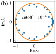
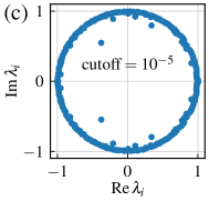
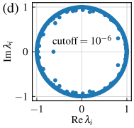
Figure 21: DMD parameters in the case of the unequal-time onsite transverse spin-spin correlation function in the 1D transverse-field Ising model with noise. (a) Singular values $\sigma_{i}$ of the truncated SVD of the matrix $X_{0}$. Eigenvalues $\lambda_{i}$ of the matrix $\tilde{A}$ are plotted in the complex plane for cutoff (b) $\epsilon=10^{-4}$, (c) $\epsilon=10^{-5}$, and (d) $\epsilon=10^{-6}$.

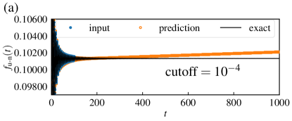
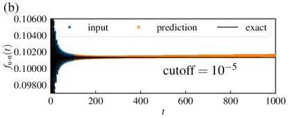
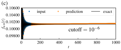
Figure 22: DMD prediction of the unequal-time onsite transverse spin-spin correlation function in the 1D transverse-field Ising model with noise. The cutoff is set to (a) $\epsilon=10^{-4}$, (b) $\epsilon=10^{-5}$, and (c) $\epsilon=10^{-6}$.

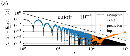
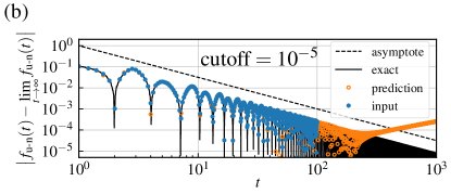
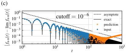
Figure 23: DMD prediction of the unequal-time onsite transverse spin-spin correlation function in the 1D transverse-field Ising model with noise in the logarithmic scale. The cutoff parameters are the same as those in Fig. 22.

Appendix B Fourier-transformed correlation function obtained by the DMD prediction in the logarithmic scale

In Sec. III.1, we predict the Fourier-transformed correlation function in the 2D transverse-field Ising model by the DMD. To carefully examine the difference between the exact result and the DMD prediction, we plot it in the logarithmic scale in Fig. 19.

The DMD prediction reproduces the exact peak positions when the absolute value of the Fourier-transformed correlation function is larger than $10\%$ of the maximum value of the exact result $\max_{\omega>0}|\tilde{f}(\omega)|$. This result indicates that the DMD method can be used to extract the physically relevant information from the short-time correlation function.

On the other hand, the DMD prediction fails to reproduce the exact peak positions with small amplitudes. These spiky structures with small intensities originate from the finite-size effect. When the system size is small, the correlation function shows a recurrence at a time scale proportional to the linear size of the system. The dominant peaks in the Fourier spectrum is mainly determined by the short-time dynamics of the correlation function until the recurrence time. As the system size increases, the number of peaks in the Fourier spectrum increases, and accumulates gradually to form a smooth curve. In the thermodynamic limit then, we would observe a continuous spectrum aside from some dominant peaks or kinks in the Fourier spectrum, just as in the case of the 1D transverse-field Ising model on an infinite chain [see Fig. 9(a)]. We may be able to reproduce such a nearly smooth curve in the Fourier spectrum when the correlation function in a sufficiently large system for a sufficiently long time is available as the input data for the DMD, although obtaining such input data is practically not feasible for the nonintegrable 2D transverse-field Ising model.

Appendix C Effects of shifting the origin of the time series

In Sec. III.2, the correlation function in the 1D transverse-field Ising model is estimated by the DMD by taking the time interval of $t_{\rm input}$ immediately after the sudden quench. This choice can be quantitatively improved by shifting the origin of the time series. This is because data just after $t=0$ are strongly influenced by the initial transient region.

We show the DMD prediction when the origin of the time series is shifted by $t_{\rm shift}=200$ in Fig. 20. In the logarithmic scale, the DMD prediction with the shifted origin looks reproducing the overall behavior of the exact result as much as the case without shifting the origin [compare Fig. 8(b) and Fig. 20(b)]. However, when one looks into more details, the DMD prediction better reproduces the exact result even up to $t=700$. By comparing the data for $t-t_{\rm shift}\in[400,510]$ with and without shifting the origin [see Fig. 8(e) and Fig. 20(e)], we can see a substantial improvement in the DMD prediction.

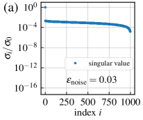
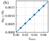
Figure 24: Singular values $\sigma_{i}$ of the truncated SVD of the matrix $X_{0}$ in the case of a constant function with noise $\epsilon_{\rm noise}$. We choose the parameters $M=1000$ and $N=2M$ for the $M\times(N-M)$ matrix $X_{0}$. (a) Normalized singular values $\sigma_{i}/\sigma_{0}$ for $\epsilon_{\rm noise}=0.03$. (b) Noise level $\epsilon_{\rm noise}$ dependence of $(M/2)$th normalized singular values $\sigma_{M/2}/\sigma_{0}$.

Appendix D Effects of noise in input data with damping

In Sec. III.3, we have discussed the effects of noise in input data without damping on the DMD prediction. There, we have found that the DMD prediction keeps up accuracy up to a certain level of the noise level (typically less than a few percent of the maximum value of input data). Here, the effects is examined by adding the noise that decays following a power law along with the main input when the main dynamics is governed by damping.

For this purpose, we employ the 1D transverse-field Ising model with damping as in Sec. III.2. When the noise level is larger than the amplitude of the correlation function, the DMD prediction clearly fails to reproduce the exact result. Therefore, in the case with damping, we add a small amount of noise which is nearly proportional to the amplitude of the correlation function. We prepare time-series data $f_{\rm u\text{-}n}(t)$ affected by such a relative noise $\eta(t)$, which is chosen to be Gaussian and white random variables with zero mean and time-dependent variance $[\sigma_{\rm noise}(t)]^{2}$. The standard deviation $\sigma_{\rm noise}(t)$ is chosen to be

$$\sigma_{\rm noise}(t)=\epsilon_{\rm noise}|f_{\rm orig}(0)|t^{-3/2},$$ (28)

with a small positive parameter $\epsilon_{\rm noise}$ that controls the noise level. The value $|f_{\rm orig}(0)|$ corresponds to the amplitude of the original correlation function at $t=0$, which is $1/4$ in the present case. Then, the time-series data $f_{\rm u\text{-}n}(t)$ affected by noise $\eta(t)$ is given by

$$f_{\rm u\text{-}n}(t)=|C^{xx}_{\rm uneq}(r=0,t)|+\eta(t),$$ (29)

where $C^{xx}_{\rm uneq}(r=0,t)$ is defined in Eq. (III.2). We set $\epsilon_{\rm noise}=0.01$ hereafter.

For the DMD, we choose the same parameters as those in Sec. III.2. Just as in the case without damping, the singular values $\sigma_{i}$ of the matrix $\bm{X}_{0}$ constructed from the input data with damping exhibit a plateau-like structure [See Fig. 21(a)]. We gradually decrease the cutoff parameter $\epsilon$ and examine the eigenvalues $\lambda_{i}$ of the matrix $\bm{A}$ [see Fig. 21(b-d)]. As for $\epsilon\gtrsim 10^{-6}$, $|\lambda_{i}|$ is found to be smaller than or equal to unity. When $\epsilon$ is decreased further, the divergence of time-series data is observed for $t\approx 10^{3}$ because of some $|\lambda_{i}|$ slightly exceeding unity. We thus choose $\epsilon\geq 10^{-6}$ as the cutoff parameter. This cutoff parameter is comparable to the value of $\sigma_{i}/\sigma_{0}$ at which the plateau-like structure appears. The corresponding rank of the truncated SVD for $\epsilon=10^{-6}$ is $R=2088$.

We show the DMD prediction in Fig. 22. As the cutoff parameter $\epsilon$ is decreased, the DMD prediction gradually reproduces the long-time behavior of the exact result. When $\epsilon=10^{-6}$, the predicted correlation function nearly converges to a constant value, which is consistent with the exact result.

To see tiny damped oscillatory behavior around the constant $f_{\rm u\text{-}n}(t)\approx 0.101$, we have examined the DMD prediction in the logarithmic scale: The predicted power-law decay to the constant becomes extended to a longer time as the cutoff parameter $\epsilon$ is decreased and progressively approaches the exact power-decay (see Fig. 23). However, even when $\epsilon=10^{-6}$, the DMD prediction for $t\gtrsim 200$ starts deviating from the exact result and from the asymptotic $t^{-3/2}$ scaling. If one is concerned with this tiny damped time dependence away from the constant, the DMD can predict the time evolution of the correlation function up to approximately twice the duration of the input data. In this regard, it is rather difficult to further improve the DMD prediction when input data with damping are affected by noise. Nevertheless, the essential and overall damping to the constant is well captured.

Appendix E Estimating the noise level from singular values

In Sec. III.3, we examine the effects of noise in input data and find that singular values of the matrix $\bm{X}_{0}$ constructed from the input data exhibit a plateau-like structure. In this section, by taking a simpler example of noisy input data, we show that the position of the plateau is proportional to the noise level in input data.

To get insight into the plateau-like structure observed in the singular values for noisy input data, we consider the case where the original input data without noise is a constant function, $f_{\rm orig}(t)=1$. We prepare time-series data $f_{\rm n}(t)$ affected by noise $\eta(t)$, which is chosen to be Gaussian white random variables with zero mean and the standard deviation $\sigma_{\rm noise}=\epsilon_{\rm noise}$. Then, the time-series data is given by $f_{\rm n}(t)=1+\eta(t)$. We choose the parameters $M=1000$ and $N=2M$ as in Sec. III.3 and controls the noise level $\epsilon_{\rm noise}=0.01,0.02,\dots,0.06$.

We show the normalized singular values $\sigma_{i}/\sigma_{0}$ for $\epsilon_{\rm noise}=0.03$ in Fig. 24(a). We observe a plateau-like structure just as in the case of the correlation function in the 2D transverse-field Ising model with noise in Sec. III.3. For the same noise level $\epsilon_{\rm noise}$, the position of the plateau is nearly the same between the time series of the constant function and those of the correlation function [compare Fig. 24(a) and Fig. 11(a)]. The only major difference is that, for the time series of the constant function, the largest singular value $\sigma_{0}$ is much larger than the second largest singular value $\sigma_{1}$. This result can be understood in the zero-noise limit, where the matrix $\bm{X}_{0}$ becomes an all-ones matrix. The singular values of the all-ones matrix are zero except for the largest singular value $\sigma_{0}$. The noise shifts the zero singular values to nonzero but small values.

The position of the plateau in the singular values is correlated with the noise level $\epsilon_{\rm noise}$. As shown in Fig. 24(b), the singular values $\sigma_{i}$ at the middle ($i=M/2$) corresponding to the plateau region is found to be proportional to $\epsilon_{\rm noise}$. They satisfy $\sigma_{M/2}\approx 0.025\epsilon_{\rm noise}$. Although the coefficient would be subject to change depending on parameters $M$ and $N$, this proportionality is expected to hold even for more general time-series data affected by noise. Therefore, we can estimate the noise level $\epsilon_{\rm noise}$ from the position of the plateau in the singular values $\sigma_{i}$ even when we do not know to what extent the original input data are affected by noise. This would be useful when estimating the noise of the experimental data.

References

- Hu et al. [2014] W. Hu, S. Kaiser, D. Nicoletti, C. R. Hunt, I. Gierz, M. C. Hoffmann, M. Le Tacon, T. Loew, B. Keimer, and A. Cavalleri, Optically enhanced coherent transport in YBa2Cu3O6.5 by ultrafast redistribution of interlayer coupling, Nat. mater. 13, 705 (2014).
- Kaiser et al. [2014] S. Kaiser, C. R. Hunt, D. Nicoletti, W. Hu, I. Gierz, H. Y. Liu, M. Le Tacon, T. Loew, D. Haug, B. Keimer, and A. Cavalleri, Optically induced coherent transport far above in underdoped YBa2Cu3O6+δ, Phys. Rev. B 89, 184516 (2014).
- Cheneau et al. [2012] M. Cheneau, P. Barmettler, D. Poletti, M. Endres, P. Schauß, T. Fukuhara, C. Gross, I. Bloch, C. Kollath, and S. Kuhr, Light-cone-like spreading of correlations in a quantum many-body system, Nature 481, 484 (2012).
- Takasu et al. [2020] Y. Takasu, T. Yagami, H. Asaka, Y. Fukushima, K. Nagao, S. Goto, I. Danshita, and Y. Takahashi, Energy redistribution and spatio-temporal evolution of correlations after a sudden quench of the Bose-Hubbard model, Sci. Adv. 6, eaba9255 (2020).
- Schollwöck [2011] U. Schollwöck, The density-matrix renormalization group in the age of matrix product states, Ann. Phys. 326, 96 (2011).
- Kshetrimayum et al. [2017] A. Kshetrimayum, H. Weimer, and R. Orús, A simple tensor network algorithm for two-dimensional steady states, Nat. Commun. 8, 1291 (2017).
- Czarnik et al. [2019] P. Czarnik, J. Dziarmaga, and P. Corboz, Time evolution of an infinite projected entangled pair state: An efficient algorithm, Phys. Rev. B 99, 035115 (2019).
- Hubig and Cirac [2019] C. Hubig and J. I. Cirac, Time-dependent study of disordered models with infinite projected entangled pair states, SciPost Phys. 6, 31 (2019).
- Hubig et al. [2020] C. Hubig, A. Bohrdt, M. Knap, F. Grusdt, and J. I. Cirac, Evaluation of time-dependent correlators after a local quench in iPEPS: hole motion in the t-J model, SciPost Phys. 8, 21 (2020).
- Schmitt et al. [2022] M. Schmitt, M. M. Rams, J. Dziarmaga, M. Heyl, and W. H. Zurek, Quantum phase transition dynamics in the two-dimensional transverse-field Ising model, Sci. Adv. 8, eabl6850 (2022).
- Kaneko and Danshita [2022] R. Kaneko and I. Danshita, Tensor-network study of correlation-spreading dynamics in the two-dimensional Bose-Hubbard model, Commun. Phys. 5, 65 (2022).
- Kaneko and Danshita [2023] R. Kaneko and I. Danshita, Dynamics of correlation spreading in low-dimensional transverse-field Ising models, Phys. Rev. A 108, 023301 (2023).
- Carleo et al. [2012] G. Carleo, F. Becca, M. Schiró, and M. Fabrizio, Localization and glassy dynamics of many-body quantum systems, Sci. rep. 2, 243 (2012).
- Carleo et al. [2014] G. Carleo, F. Becca, L. Sanchez-Palencia, S. Sorella, and M. Fabrizio, Light-cone effect and supersonic correlations in one- and two-dimensional bosonic superfluids, Phys. Rev. A 89, 031602(R) (2014).
- Ido et al. [2015] K. Ido, T. Ohgoe, and M. Imada, Time-dependent many-variable variational Monte Carlo method for nonequilibrium strongly correlated electron systems, Phys. Rev. B 92, 245106 (2015).
- Carleo and Troyer [2017] G. Carleo and M. Troyer, Solving the quantum many-body problem with artificial neural networks, Science 355, 602 (2017).
- Nomura et al. [2017] Y. Nomura, A. S. Darmawan, Y. Yamaji, and M. Imada, Restricted Boltzmann machine learning for solving strongly correlated quantum systems, Phys. Rev. B 96, 205152 (2017).
- Ido et al. [2017] K. Ido, T. Ohgoe, and M. Imada, Correlation-induced superconductivity dynamically stabilized and enhanced by laser irradiation, Sci. Adv. 3, e1700718 (2017).
- Schmitt and Heyl [2020] M. Schmitt and M. Heyl, Quantum Many-Body Dynamics in Two Dimensions with Artificial Neural Networks, Phys. Rev. Lett. 125, 100503 (2020).
- Barthel et al. [2009] T. Barthel, U. Schollwöck, and S. R. White, Spectral functions in one-dimensional quantum systems at finite temperature using the density matrix renormalization group, Phys. Rev. B 79, 245101 (2009).
- Goto et al. [2016] S. Goto, S. Kurihara, and D. Yamamoto, Incommensurate spiral magnetic order on anisotropic triangular lattice: Dynamical mean-field study in a spin-rotating frame, Phys. Rev. B 94, 245145 (2016).
- Huang et al. [2023] H.-Y. Huang, S. Chen, and J. Preskill, Learning to Predict Arbitrary Quantum Processes, PRX Quantum 4, 040337 (2023).
- [23] N. Mohseni, J. Shi, T. Byrnes, and M. Hartmann, Deep learning of many-body observables and quantum information scrambling, arXiv:2302.04621 .
- [24] G. Cemin, F. Carnazza, S. Andergassen, G. Martius, F. Carollo, and I. Lesanovsky, Inferring interpretable dynamical generators of local quantum observables from projective measurements through machine learning, arXiv:2306.03935 .
- [25] Z.-W. Wang and Z.-M. Wang, Time series prediction of open quantum system dynamics, arXiv:2401.06380 .
- Schmid and Sesterhenn [2008] P. J. Schmid and J. Sesterhenn, Dynamic Mode Decomposition of numerical and experimental data, in 61st Annual Meeting of the APS Division of Fluid Dynamics (American Physical Society, 2008).
- Rowley et al. [2009] C. W. Rowley, I. Mezić, S. Bagheri, P. Schlatter, and D. S. Henningson, Spectral analysis of nonlinear flows, Journal of Fluid Mechanics 641, 115 (2009).
- Schmid [2010] P. J. Schmid, Dynamic mode decomposition of numerical and experimental data, J. Fluid Mech. 656, 5 (2010).
- Tu et al. [2014] J. H. Tu, C. W. Rowley, D. M. Luchtenburg, S. L. Brunton, and J. N. Kutz, On dynamic mode decomposition: Theory and applications, J. Comput. Dyn. 1, 391 (2014).
- Kutz et al. [2016] J. N. Kutz, S. L. Brunton, B. W. Brunton, and J. L. Proctor, Dynamic mode decomposition: data-driven modeling of complex systems (SIAM, Philadelphia, PA, USA, 2016).
- Brunton and Kutz [2019] S. L. Brunton and J. N. Kutz, Data-driven science and engineering: Machine learning, dynamical systems, and control (Cambridge University Press, Cambridge, England, 2019).
- Schmid [2022] P. J. Schmid, Dynamic Mode Decomposition and Its Variants, Annu. Rev. Fluid Mech. 54, 225 (2022).
- [33] L. Pogorelyuk and C. W. Rowley, Clustering of Series via Dynamic Mode Decomposition and the Matrix Pencil Method, arXiv:1802.09878 .
- Sarkar et al. [1980] T. Sarkar, J. Nebat, D. Weiner, and V. Jain, Suboptimal approximation/identification of transient waveforms from electromagnetic systems by pencil-of-function method, IEEE Trans. Antennas Propag. 28, 928 (1980).
- Hua and Sarkar [1990] Y. Hua and T. K. Sarkar, Matrix pencil method for estimating parameters of exponentially damped/undamped sinusoids in noise, IEEE Trans. Signal Process. 38, 814 (1990).
- Sarkar and Pereira [1995] T. K. Sarkar and O. Pereira, Using the matrix pencil method to estimate the parameters of a sum of complex exponentials, IEEE Trans. Antennas Propag. 37, 48 (1995).
- Goldschmidt et al. [2021] A. Goldschmidt, E. Kaiser, J. L. Dubois, S. L. Brunton, and J. N. Kutz, Bilinear dynamic mode decomposition for quantum control, New J. Phys. 23, 033035 (2021).
- Sakata et al. [2021] I. Sakata, T. Sakata, K. Mizoguchi, S. Tanaka, G. Oohata, I. Akai, Y. Igarashi, Y. Nagano, and M. Okada, Complex energies of the coherent longitudinal optical phonon–plasmon coupled mode according to dynamic mode decomposition analysis, Sci. Rep. 11, 23169 (2021).
- Kawashima et al. [2021] T. Kawashima, H. Shouno, and H. Hino, Bayesian dynamic mode decomposition with variational matrix factorization, in Proc. AAAI Conf. Artif. Intell., Vol. 35 (2021) pp. 8083–8091.
- Yin et al. [2022] J. Yin, Y.-h. Chan, F. H. da Jornada, D. Y. Qiu, S. G. Louie, and C. Yang, Using dynamic mode decomposition to predict the dynamics of a two-time non-equilibrium Green’s function, J. Comput. Sci. 64, 101843 (2022).
- Yin et al. [2023] J. Yin, Y.-h. Chan, F. H. da Jornada, D. Y. Qiu, C. Yang, and S. G. Louie, Analyzing and predicting non-equilibrium many-body dynamics via dynamic mode decomposition, J. Comput. Sci. 477, 111909 (2023).
- Baddoo et al. [2023] P. J. Baddoo, B. Herrmann, B. J. McKeon, J. Nathan Kutz, and S. L. Brunton, Physics-informed dynamic mode decomposition, Proc. R. Soc. A 479, 20220576 (2023).
- Reeves et al. [2023] C. C. Reeves, J. Yin, Y. Zhu, K. Z. Ibrahim, C. Yang, and V. c. v. Vlček, Dynamic mode decomposition for extrapolating nonequilibrium Green’s-function dynamics, Phys. Rev. B 107, 075107 (2023).
- Gu et al. [2024] M. Gu, Y. Lin, V. C. Lee, and D. Y. Qiu, Probabilistic forecast of nonlinear dynamical systems with uncertainty quantification, Phys. D: Nonlinear Phenom. 457, 133938 (2024).
- [45] A. Hunstig, S. Peitz, H. Rose, and T. Meier, Accelerating the analysis of optical quantum systems using the Koopman operator, arXiv:2310.16578 .
- [46] I. Maliyov, J. Yin, J. Yao, C. Yang, and M. Bernardi, Dynamic mode decomposition of nonequilibrium electron-phonon dynamics: accelerating the first-principles real-time Boltzmann equation, arXiv:2311.07520 .
- Steffens et al. [2017] A. Steffens, P. Rebentrost, I. Marvian, J. Eisert, and S. Lloyd, An efficient quantum algorithm for spectral estimation, New J. Phys. 19, 033005 (2017).
- [48] Y. Shen, D. Camps, A. Szasz, S. Darbha, K. Klymko, D. B. Williams-Young, N. M. Tubman, and R. V. Beeumen, Estimating Eigenenergies from Quantum Dynamics: A Unified Noise-Resilient Measurement-Driven Approach, arXiv:2306.01858 .
- [49] N. Gomes, J. Yin, S. Niu, C. Yang, and W. A. de Jong, A hybrid method for quantum dynamics simulation, arXiv:2307.15231 .
- [50] Y. Mizuno and T. Komatsuzaki, Quantum Algorithm for Dynamic Mode Decomposition and Matrix Eigenvalue Decomposition with Complex Eigenvalues, arXiv:2310.17783 .
- [51] A. Szasz, E. Younis, and W. A. de Jong, Ground state energy and magnetization curve of a frustrated magnetic system from real-time evolution on a digital quantum processor, arXiv:2401.03015 .
- Tommet and Huber [1975] T. N. Tommet and D. L. Huber, Dynamical correlation functions of the transverse spin and energy density for the one-dimensional spin-½ Ising model with a transverse field, Phys. Rev. B 11, 450 (1975).
- Müller and Shrock [1984] G. Müller and R. E. Shrock, Dynamic correlation functions for one-dimensional quantum-spin systems: New results based on a rigorous approach, Phys. Rev. B 29, 288 (1984).
- Rossini et al. [2009] D. Rossini, A. Silva, G. Mussardo, and G. E. Santoro, Effective Thermal Dynamics Following a Quantum Quench in a Spin Chain, Phys. Rev. Lett. 102, 127204 (2009).
- Rossini et al. [2010] D. Rossini, S. Suzuki, G. Mussardo, G. E. Santoro, and A. Silva, Long time dynamics following a quench in an integrable quantum spin chain: Local versus nonlocal operators and effective thermal behavior, Phys. Rev. B 82, 144302 (2010).
- Halko et al. [2011] N. Halko, P.-G. Martinsson, and J. A. Tropp, Finding structure with randomness: Probabilistic algorithms for constructing approximate matrix decompositions, SIAM review 53, 217 (2011).
- Perales and Vidal [2008] A. Perales and G. Vidal, Entanglement growth and simulation efficiency in one-dimensional quantum lattice systems, Phys. Rev. A 78, 042337 (2008).
- Rieger and Kawashima [1999] H. Rieger and N. Kawashima, Application of a continuous time cluster algorithm to the two-dimensional random quantum Ising ferromagnet, Eur. Phys. J. B 9, 233 (1999).
- Blöte and Deng [2002] H. W. J. Blöte and Y. Deng, Cluster Monte Carlo simulation of the transverse Ising model, Phys. Rev. E 66, 066110 (2002).
- Kaneko et al. [2021] R. Kaneko, Y. Douda, S. Goto, and I. Danshita, Reentrance of the Disordered Phase in the Antiferromagnetic Ising Model on a Square Lattice with Longitudinal and Transverse Magnetic Fields, J. Phys. Soc. Jpn. 90, 073001 (2021).
- Weinberg and Bukov [2017] P. Weinberg and M. Bukov, QuSpin: a Python Package for Dynamics and Exact Diagonalisation of Quantum Many Body Systems part I: spin chains, SciPost Phys. 2, 003 (2017).
- Weinberg and Bukov [2019] P. Weinberg and M. Bukov, QuSpin: a Python Package for Dynamics and Exact Diagonalisation of Quantum Many Body Systems. Part II: bosons, fermions and higher spins, SciPost Phys. 7, 20 (2019).
- Rasmussen and Williams [2006] C. E. Rasmussen and C. K. I. Williams, Gaussian processes for machine learning (The MIT Press, Cambridge, MA, USA, 2006).
- Pedregosa et al. [2011] F. Pedregosa, G. Varoquaux, A. Gramfort, V. Michel, B. Thirion, O. Grisel, M. Blondel, P. Prettenhofer, R. Weiss, V. Dubourg, J. Vanderplas, A. Passos, D. Cournapeau, M. Brucher, M. Perrot, and E. Duchesnay, Scikit-learn: Machine Learning in Python, J. Mach. Learn Res. 12, 2825 (2011).
- Pfeuty [1970] P. Pfeuty, The one-dimensional Ising model with a transverse field, Ann. Phys. 57, 79 (1970).
- McCoy et al. [1971] B. M. McCoy, E. Barouch, and D. B. Abraham, Statistical Mechanics of the Model. IV. Time-Dependent Spin-Correlation Functions, Phys. Rev. A 4, 2331 (1971).
- [67] E. Brochu, V. M. Cora, and N. de Freitas, A Tutorial on Bayesian Optimization of Expensive Cost Functions, with Application to Active User Modeling and Hierarchical Reinforcement Learning, arXiv:1012.2599 .
- [68] J. Snoek, H. Larochelle, and R. P. Adams, Practical Bayesian Optimization of Machine Learning Algorithms, arXiv:1206.2944 .
- Nogueira [2014] F. Nogueira, Bayesian Optimization: Open source constrained global optimization tool for Python (2014).