Spin cones in random-field XY models
Abstract
We determine the arrangement of spins in the ground state of the XY model with quenched, random fields, on a fully connected graph. Two types of disordered fields are considered, namely randomly oriented magnetic fields, and randomly oriented crystal fields. Orientations are chosen from a uniformly isotropic distribution, but disorder fluctuations in each realization of a finite system lead to a breaking of rotational symmetry. The result is an interesting pattern of spin orientations, found by solving a system of coupled, nonlinear equations within perturbation theory and also by exact numerical continuation. All spins lie within a cone for small enough ratio of field to coupling strength, with an interesting distribution of spin orientations, with peaks at the cone edges. The orientation of the cone depends strongly on the realization of disorder, but the opening angle does not. In the case of random magnetic fields, the cone angle widens as the ratio increases till a critical value at which there is a first order phase transition and the cone disappears. With random crystal fields, there is no phase transition and the cone angle approaches for large values of the ratio. At finite low temperatures, Monte-Carlo simulations show that the formation of a cone and its subsequent alignment along the equilibrium direction occur on two different time scales.
I Introduction
Frozen-in or quenched disorder is known to have strong effects on the thermodynamic properties of statistical systems. In particular, the interplay of frozen-in randomness with cooperative interactions can have a profound influence on the nature of ordered states of spin systems, and lead to new types of patterning. Customarily, theoretical studies are carried out by averaging over different realizations of disorder in the thermodynamic limit of the number of spins . However, this procedure can mask interesting macroscopic patterns that emerge from the competition between quenched randomness and cooperativity in a system with large but finite . We show this by explicitly determining the exact ground state of an XY model in the presence of randomly oriented fields. In each realization of disorder, we demonstrate that there is an interesting fan-like arrangement of spins with a robust cone angle, and an interesting distribution of spins within the cone.
The question of magnetic ordering in the presence of random fields has a long history, and remains a question of current interest. In this paper we study XY ferromagnets with long- range interactions, subject to two distinct types of locally quenched fields: random magnetic fields which promote order in different directions (the RFXY model), and random crystal fields which define a random set of easy axes for spins (the RCXY model). The RFXY model has been used to study disordered superconductors Larkin (1970); Fisher (1989); Nattermann et al. (1991) and crystal surfaces with quenched disorder Toner and DiVincenzo (1990). On the other hand, the RCXY model was proposed Harris et al. (1973) to explain the magnetic properties of amorphous materials, exemplified by rare earth compounds such as and Coey and Von Molnar (1978); Ferrer et al. (1978). The randomness of anisotropy axis orientation competes with ferromagnetic exchange and reduces the magnetization Callen et al. (1977); foo . The model has been used to understand the magnetic properties of many amorphous binary alloys Krey (1977); Alben et al. (1978); Dudka et al. (2005); Idzikowski et al. (2005), as well as nanocrystalline Hernando et al. (1995); Alvarez et al. (2020) and molecular Gîrţu et al. (2000) magnets.
The occurrence and nature of order in these systems is a central question. A general argument was given by Imry and Ma to show that a ferromagnetically ordered state cannot be sustained in less than two (four) dimensions for discrete (vector) spins Imry and Ma (1975). While a spin-glass phase is ruled out in the random-field Ising model Krzakala et al. (2010), there is no analogous result which rules out a spin-glass phase in models with continuous spins. In fact there is evidence supporting the existence of such a phase in RFXY models with short-range interaction Cardy and Ostlund (1982); Le Doussal and Giamarchi (1995). The RCXY model with short-range interaction is expected to exhibit a spin glass phase below six dimensions Aharony (1975); Pelcovits et al. (1978); Chudnovsky et al. (1986). A spin glass phase is also found in a Monte Carlo study of the 3D RCXY in infinitely strong crystal fields, in which limit it reduces to a quenched random-bond Ising model with correlated random couplings of either sign Jayaprakash and Kirkpatrick (1980). However, in higher dimensions, we expect ferromagnetism to prevail at low temperatures.
The problem for either sort of random field has been studied earlier on fully connected graphs. Infinite-range connectivity has the advantage that the free energy can be calculated exactly in the thermodynamic limit. For the RFXY model this was done recently using large deviations Sumedha and Barma (2022a), belief propagation Lupo et al. (2019) and replicas Morone and Sels (2023). The nature of the critical locus which separates the disordered phase from an ordered phase with finite magnetization depends on the distribution of random fields: with a Gaussian distribution, it is second-order throughout Morone and Sels (2023), while with randomly oriented fields of fixed magnitude (the case of interest to us), the transition becomes first order for strong fields and low temperature Sumedha and Barma (2022a). For the RCXY model, there is a similar phase transition to an ordered state, but the transition locus remains second order throughout Derrida and Vannimenus (1980); Sumedha and Barma (2022b).
Although bulk thermodynamic quantities were calculated in these treatments, the nature of spin ordering in the ferromagnetic state remained unknown even in the ground state. This is the central question we address in this paper. With randomly-pointing fields of constant magnitude drawn from an isotropic distribution, in a typical configuration, an effective field of order breaks the isotropic symmetry of the ground state. Minimization of the energy yields coupled nonlinear equations for the spin orientations. We develop a perturbative method to solve for the spin angles for small values of the ratio of field strength to the exchange, and find that they lie within a well-defined cone whose orientation varies from sample to sample, but whose opening angle is robust. Interestingly, the distribution of spins within the cone is found to be largest near the cone edges. An exact numerical treatment of the nonlinear equations confirms the perturbative results and further shows that with increasing field, there is a first order phase transition to a disordered state, as predicted in Sumedha and Barma (2022a). The cone angle increases continuously until the transition, beyond which the cone disappears. On the other hand, in the random crystal field problem, the cone angle increases continuously to 180 degrees as the strength of the crystal field goes to .
We also performed Monte Carlo simulations for both RFXY and RCXY models at low temperatures, and found that cone formation is robust. An interesting dynamics governs cone formation and settling: Formation of a well-defined cone is quick and happens on a time scale determined by the exchange coupling, while its orientation relaxes on a slower time scale set by the strength of the random field. We develop a phenomenological equation which describes this dynamics.
II The model
The RFXY model is defined by the Hamiltonian
| (1) |
where the spin is a two dimensional unit vector associated with the th site of a fully connected graph with sites. The spin at site is coupled to that at site with an energy . At every site there is a random field with site-independent strength and site-dependent direction determined by the unit vector . The unit vectors are independent and identically distributed random vectors that can lie anywhere on a unit circle with equal likelihood. The spin at site is coupled to the random field at that site with an energy .
The RCXY model is obtained by replacing the last term in the Hamiltonian (1):
| (2) |
where represents the strength of the random crystal field in the direction at site . The unit vectors are distributed uniformly as in the RFXY model. The RCXY model has an underlying Ising symmetry: the Hamiltonian is invariant under the transformation .
As mentioned earlier, the RFXY model exhibits a locus of order-disorder phase transitions in the plane, where is the temperature. The transitions are of first order in the portion of the locus lying in the low temperature regime, which is separated from the portion lying in high temperature regime, where the transitions are continuous, by a tricritical point. For the RCXY model the transitions are of second order everywhere and the critical temperature is independent of the ratio Derrida and Vannimenus (1980); Sumedha and Barma (2022b). Further, there is no phase transition to a disordered state when the ratio of field to coupling strength is varied at , in contrast to the RFXY model.
In the following sections we will be interested in the nature of the ordered state in both these models at and at temperatures close to zero. In particular, we will explore the arrangement of spins in a finite system with a given configuration of fields. Though the field-orientations are chosen from an isotropic distribution, rotational symmetry is broken for any finite .
III RFXY: Cones at zero-temperature
In this section, we explore the arrangement of spins for the RFXY model.
III.1 Perturbation theory:
An insight into the distribution of spins can be obtained by analyzing the ground state of the Hamiltonian (1) using perturbation theory. To this end, Eq. (1) is first recast in terms of the angles and that the spins and the fields , respectively, make with the -axis. The ensuing equation is then extremized with respect to , yielding the following set of equations for the ground state.
| (3) |
To solve these, we expand in powers of as
| (4) |
Note that the ’th order term is independent of , since all spins point in same direction in the limit . On substituting Eq. (4) in Eq. (3) and then expanding in powers of , we obtain the following equations at and , respectively:
| (5) | ||||
| (6) |
Note there are equations at each order. On summing the ‘first-order’ equations (5) we obtain the ’th order contribution to as
| (7) | ||||
| (8) |
This implies or , where is the angle made by
| (9) |
with the -axis. The latter solution has a higher energy and is therefore discarded. We conclude that at , all the spins point in the direction of the vector sum of the fields. Note that for any finite system size , the sum of disordered fields is of the order , which results in singling out a preferred direction , breaking rotational symmetry.

We now focus on the first order corrections , which satisfy the equations (5). However, only of these equations are linearly independent since the equations (5) add to give . The ‘missing’ equation which, together with Eq. (5), uniquely determines is obtained from the ‘second-order’ equations (6), which on summing over yield Solving this simultaneously with Eqs. (5) yields
| (10) |
where we have replaced by and
| (11) |
Replacing in Eq. (4) by Eq. (5) we get
| (12) |
to first order in .
To find the orientation of the magnetization and the distribution of spins around it to first order we write
| (13) |
where is the magnetization in the limit . To obtain the last line, we used Eq. (12) and expanded the resulting expression to first order in . The factor in the second term of Eq. (III.1) can be evaluated using Eqs. (10), (11), and (7) to obtain . The orientation of the magnetization is thus
| (14) |
to first order in . The angle that the th spin makes with is
| (15) |
where we have used Eqs. (4), (10), and (14). For random fields that are uniformly distributed over a circle, we obtain the probability distribution for as
| (16) |
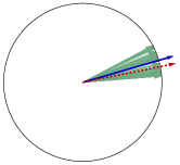
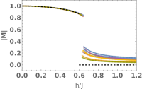
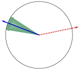
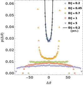
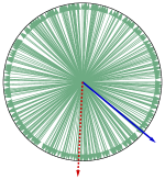
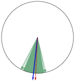
A plot of the distribution for is shown by the black line in Fig. 1e. Note that all the spins lie within a cone whose edges are given by , at which points the distribution diverges. Within the cone, the distribution is minimum at the center. The arrangement of spins in the perturbative regime, for a particular sample of size , is depicted using the green arrows confined within the circle in Fig. 1b. The red dashed arrow shows the direction of and the blue continuous arrow shows the direction of . The spin configuration shown therein corresponds to the particular field configuration shown in Fig. 1a.
Thus we see that spins are distributed within a cone whose orientation is given by Eq. (14), while the cone angle, defined as the angular separation between the spins at the two farthest edges of the cone, is given by
| (17) |
which is evident from Eq. (16). The cone orientation depends on the configuration of fields, while the cone angle does not.
III.2 Numerically continuing to higher
We now investigate how the conical arrangement of spins changes as increases. We will show that the cone angle increases continuously until a critical value , at which point there is a first order transition to a disordered state. As the critical value , the value obtained from the large deviation calculation Sumedha and Barma (2022a).
The distribution of spins is obtained by solving the equation for extremum (3) using the method of numerical continuation Eugene L. Allgower (2012). The equation is independently solved for several configurations of quenched random fields and for different values of . In particular, we choose , , , and . The procedure is briefly explained below.
First, angles are chosen independently from the interval with uniform likelihood. This fixes the directions of the quenched random fields . Now, the formula derived using the perturbation theory (12) is used to obtain an approximate solution to Eq (3) for a small value of (say, ). This solution is used as an initial guess using which we numerically continue to higher values of . (See Appendix A for further details.)
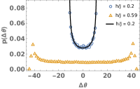
For small enough , we find that the distribution of spins is consistent with the perturbative results. The spins are confined within a cone centered along the direction of magnetization as shown in Fig. 1b. The number of spins is largest at the edges, where there is a sharp cut-off, and smallest at the center of the cone. This is demonstrated using the case of in Fig. 1e (blue circles), where the probability density is plotted against . The probability density was obtained by sampling over configurations with .
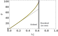
We find that the cone angle widens until the critical value is reached. Figure 1d shows the variation of for . The values of the cone angles at the phase transition are found to be , , , and degrees for , , and , respectively, on averaging over samples for each . The results are consistent with as . The distribution of spins within the cone just before the phase transition (at ) is found to be flat around the center of the cone, unlike for small (see Fig. 1e). The value of shows sample to sample fluctuation and a systematic fall as increases. We find , , , and for , , and , respectively. Note that the results are consistent with for .
The numerical continuation scheme fails at a value of slightly greater than as there is no ordered state solution to Eq. (3) at this point. The solutions that minimize the energy (1) at points beyond are the disordered ones. To access these, we numerically continue backwards in from the state in the limit . The starting guess solution to Eq. (3), obtained perturbatively, is .
There is an abrupt change in the arrangement of spins as is increased past the transition point: from being confined to a cone, for , they spread over a circle. The distribution of spins in the disordered phase for a typical configuration of fields is shown in Fig. 1c (at ). We note here that for this sample the phase transition occurs between and .
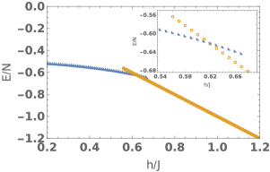
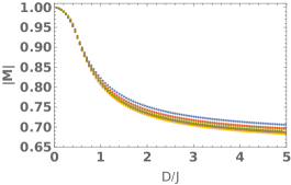
There is also a sudden jump in the magnetization at the phase transition for each sample, which is clear from the plot in Fig. 1f, indicating clearly that the system is undergoing a first order phase transition. The dashed black line therein shows the exact modulus of magnetization in the thermodynamic limit, calculated using large deviation theory in Sumedha and Barma (2022a).
The energies of the minima obtained for a typical configuration of fields using the scheme described above are plotted against in Fig. 1g. The cones and circles used as markers therein indicate that the solutions in these regions correspond to conical and disordered arrangements of spins, respectively. Note that the conical (disordered) states continue to the right (left) of the transition point, where they are no longer the global minima but are still metastable local minima of the Hamiltonian.


IV RCXY: Cones at zero-temperature
We turn to a study of the spin arrangements for the RCXY model as a function of the crystal field strength , using perturbation theory followed by numerical continuation in the non-perturbative regime.
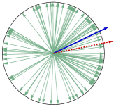
When , the arrangement of spins for the RCXY model is identical to that for the RFXY model. A typical field configuration with is shown in Fig. 2a, which is exactly the same as the configuration in Fig. 1a for the RFXY model. Figures 2b and 2c show the corresponding spin configurations at and , respectively. The red dashed (blue continuous) line shows the direction of vector sum of fields (spins).
There is a striking difference between the two models for higher values of . For instance, the distribution of spins within the cone changes and has a maximum at the center of the cone when , for the RCXY model. Further, unlike the RFXY model, there is no phase transition, and the cone is preserved for all values of . Moreover, the cone does not align along in the limit , in contrast to the RFXY model.
The calculation proceeds along the lines spelled out in Sec. III. To first order, the perturbative solution for that minimize the RCXY Hamiltonian (2) for small values of is
| (18) |
where is given by
| (19) |
and
| (20) |
Equation (19) yields four solutions for , namely , and , where is defined as half of the angle that the vector makes with the -axis. The first two and the last two solutions are degenerate. However, the latter pair has higher energy and is therefore discarded.
Note that in the case of RCXY, the solutions for extrema are always two-fold degenerate as the Hamiltonian is invariant under the transformation . This implies that there are at least two global minima, and our calculations indicate that there are only two for finite values of . In the following, we focus on one of the two minima.
The perturbative solution leads to a magnetization
| (21) |
to first order in . It is straightforward to see that orients along , leading to the following probability distribution for the deviation of a spin from .
| (22) |
Thus, as for the RFXY model, spins are confined within a cone, at whose center the distribution is minimum and at whose edges the distribution diverges. The cone angle is given by .
Beyond the perturbative regime, our numerical studies show that the spins remain confined to a cone, but the distribution becomes flat within the cone at . As is increased further, the distribution develops a maximum at the center of the cone. Asymptotically, as , we expect the distribution to become flat again. Fig. 2e shows the probability density at various values of .
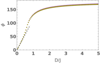
The cone angle widens with as shown in Fig. 2d, initially linearly but the widening slows down when . As , the cone angle when is infinite. This can be conceptualized as follows. In the limit the fields will be distributed uniformly everywhere over the circle, and as the second term in the Hamiltonian (2) will dominate forcing each spin to lie on the easy axes pointing either along the direction of the respective field or opposite to it. Thus we have an Ising degree of freedom at each site. However, the term would prefer the spins to be parallel to each other resulting in the spins spanning a hemisphere. We note here that the hemispherical distribution of spins in the limit has been pointed out in Callen et al. (1977).
Figure 2f shows the behavior of magnetization as a function of . The magnetization decreases smoothly and there is no phase transition. As magnetization in the thermodynamic limit Sumedha and Barma (2022b).

V Cones and dynamics at
Here, we use Monte-Carlo simulations to address the question of robustness of the cone and the spin distribution at equilibrium for the RFXY model at . The RCXY model shows similar equilibrium features, and is therefore not discussed separately. We show that the spin distribution remains similar to that at and has a two-peaked structure below a characteristic temperature determined by the field.
We also perform Monte-Carlo simulations below this temperature to study the dynamics of the approach to the ordered spin state starting from a typical random initial configuration of spins. We restrict ourselves to the RFXY model in this case.
V.1 Equilibrium cones
To first order in , the energy per spin in the ground state is given by
| (23) |
which is obtained by using Eqs. (1) and (12). The contribution coming from the randomly disordered fields is . Since ’s are independent random vectors distributed uniformly over a unit circle, we have
| (24) |
implying, . Thus disorder brings into play a characteristic temperature . We performed Monte-Carlo simulations at and according to the following procedure.
First, a random field configuration is realized by choosing field-angles independently and uniformly from the interval . An initial spin configuration is chosen by assigning a set of angles in the same fashion. The angles are now evolved in steps using the Metropolis algorithm. Each step consists of micro-steps, at each of which a particular is chosen at random and varied by an angle that is chosen randomly and uniformly from the interval . This changes the spin angles, say, from to . At the end of a step, if the new spin configuration lowers the energy (1), it is accepted. Otherwise it is accepted with a probability , where . Each such step corresponds to one unit time.
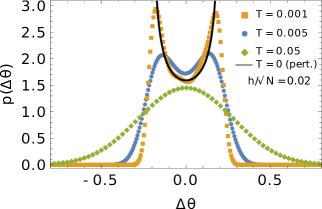
From the simulations, we find that the equilibrium distributions of spins within the cone have different characteristics for and , as shown in Fig. 3. For , the distribution is similar to that at , with maxima towards the edges of the cone and minimum at the center, whereas for , the distribution is a Gaussian peaked at the center of the cone. The equilibrium distributions of spins exhibit the same features for the RCXY model also, with the characteristic temperature .
V.2 Low temperature dynamics
We now study the dynamics of spins in the ordered state using analytical and Monte-Carlo methods, restricting ourselves to .
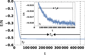
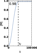
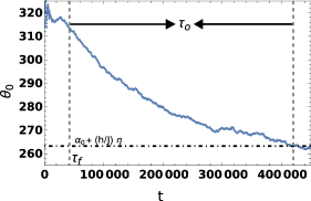
We find that the evolution of spins from a typical random initial configuration to the equilibrium state is characterized by two time scales. In the initial, shorter time scale , the randomly oriented spins come together and form a cone, while on the second longer time scale , the cone rotates and orients along the equilibrium direction. Figure 4 shows illustrations of evolution of the spin configuration, and plots depicting the evolution of the magnitude and the orientation of magnetization and the evolution of energy for a typical field configuration and initial spin configuration.
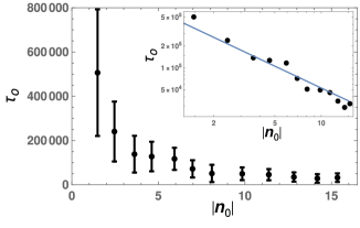
We find that the cone formation time depends primarily on , while the cone-orientation time is set by . Further, depends on . The larger the value of , the shorter is the orientation time. This is evident from Fig. 5, which shows the cone orientation time for different field configurations, each with a different value of . Note that in practice, we calculate as the time at which the value of first reaches and as the time at which orients at an angle , which is the orientation of according to the perturbation theory (14).
We write a phenomenological dynamical equation to describe the evolution of the orientation of once the cone has formed:
| (25) |
where the effects of thermal fluctuations are neglected. Since we are interested primarily in the orientation of the cone, we neglect the spread of spins within the cone and write for all . This simplification is justified for small enough when the spins point more or less along the same direction once the cone has formed. Thus, Eq (1) becomes
| (26) | ||||
| (27) |
where denotes the orientation of . Defining , the sum in the second term in Eq. (27) can be rewritten as
| (28) |
where we used the results and . Solving for using Eqs. (25), (27), and (28), we obtain
| (29) |
From the above we see that the relaxation time which is corroborated by the numerical results (see Fig. 5).
VI Conclusion
The ordered states in the RFXY and the RCXY models show interesting arrangements of spins, which break rotational symmetry for any finite . In the ground state, the spins are confined within a two-dimensional cone, whose angle and orientation are determined by the ratio of disorder to coupling strength. The distribution of spins within the cone is sensitive to temperature, and shows very different features for and . The dynamics of spins relaxing to equilibrium is characterized by two time scales, namely, the cone formation time and the cone orientation time.
Note that rotational symmetry is restored only if is strictly infinite: the ground state energy per spin becomes insensitive to the orientation of in that limit. Further, our preliminary analysis of the dynamics suggests that , where , implying that the cone orientation time diverges as . The cone formation time is also sensitive to . It would be interesting to track the -dependence of these times.
Another physically relevant question is: what is the effect of a uniform external field on the cones and arrangement of spins, as well as on the phase diagram? A preliminary study, based on the extension of our numerical continuation techniques to this problem, suggests that at , the external field reorients the cone, with a possible first order phase transition — from an ordered state to a different ordered state.
We expect many of the qualitative features of the RFXY and RCXY models, like the existence of a cone, to remain valid for the case of Heisenberg spins that can lie anywhere on a unit sphere.
VII Acknowledgment
We thank Arghya Das, Smarajit Karmakar, and Sumedha for fruitful discussions. M.B. acknowledges the support of the Indian National Science Academy(INSA). We acknowledge the support of the Department of Atomic Energy, Government of India, under Project Identification No. RTI 4007.
Appendix A Numerical continuation
Here, we explicitly lay down the procedure for solving the nonlinear Eqs. (3) numerically.
The left hand side of Eq. (3) , for , constitute a set of continuously differentiable functions of the variables and the parameter , for a fixed and field angles . It is useful to write down Eq. (3) in terms of here:
| (30) |
If for a set of values , for every , then that set is called a solution-point.
If there exists a solution-point for which
| (31) |
where the subscript indicates that the derivatives are to be taken at , then there also exists a unique set of solution-points for values of in the neighborhood of , by implicit function theorem. Such a solution point is referred to as regular.
If we know a regular solution-point , we can find a nearby solution-point approximately by incrementing the parameter by a small number to obtain and then finding that solves the linearized version of Eq. (30), which is
| (32) |
The above equation can be solved easily to obtain , and hence . The accuracy of the approximate solution can be improved by using any of the familiar iterative schemes, such as the Newton-Raphson or the Secant method. In this paper we have used the inbuilt FindRoot function in Mathematica.
If the new solution point is also regular, we can repeat the above scheme to find the next solution point , and so forth. Alternate methods have to be used if a solution-point is not regular. For solving Eq. (3), we start from the perturbative solution (12) and not from the solution at because the latter is not a regular solution-point. However, the subsequent solution points that correspond to the minima of the Hamiltonian (1) are regular, and therefore no alternate schemes had to be used. Further, the absence of non-regular solution-points implies that there are no bifurcations or folds at any of these points.
References
- Larkin (1970) A. I. Larkin, Sov. Phys. JETP 31, 784 (1970).
- Fisher (1989) M. P. A. Fisher, Phys. Rev. Lett. 62, 1415 (1989).
- Nattermann et al. (1991) T. Nattermann, I. Lyuksyutov, and M. Schwartz, Europhys. Lett. 16, 295 (1991).
- Toner and DiVincenzo (1990) J. Toner and D. P. DiVincenzo, Phys. Rev. B 41, 632 (1990).
- Harris et al. (1973) R. Harris, M. Plischke, and M. J. Zuckermann, Phys. Rev. Lett. 31, 160 (1973).
- Coey and Von Molnar (1978) J. Coey and S. Von Molnar, J. Phys. (Paris) 39, 327 (1978).
- Ferrer et al. (1978) R. Ferrer, R. Harris, D. Zobin, and M. Zuckermann, Solid State Commun. 26, 451 (1978).
- Callen et al. (1977) E. Callen, Y. J. Liu, and J. R. Cullen, Phys. Rev. B 16, 263 (1977).
- (9) Disorder enters only through the random orientation of anisotropy and not its magnitude, consistent with experimental Mossbauer evidence in amorphous materials; see Ref. Sarkar et al. (1974).
- Krey (1977) U. Krey, J. Magn. Magn. Mater. 6, 27 (1977).
- Alben et al. (1978) R. Alben, J. Becker, and M. Chi, Journal of applied physics 49(3), 1653 (1978).
- Dudka et al. (2005) M. Dudka, R. Folk, and Y. Holovatch, J. Magn. Magn. Mater. 294, 305 (2005).
- Idzikowski et al. (2005) B. Idzikowski, P. Švec, and M. Miglierini, Properties and Applications of Nanocrystalline Alloys from Amorphous Precursors. NATO Science Series (Series II: Mathematics, Physcis and Chemistry), Vol. 184 (Springer Science & Business Media, 2005).
- Hernando et al. (1995) A. Hernando, M. Vázquez, T. Kulik, and C. Prados, Phys. Rev. B 51, 3581 (1995).
- Alvarez et al. (2020) K. L. Alvarez, J. M. Martín, N. Burgos, M. Ipatov, L. Domínguez, and J. González, Nanomaterials 10, 884 (2020).
- Gîrţu et al. (2000) M. A. Gîrţu, C. M. Wynn, J. Zhang, J. S. Miller, and A. J. Epstein, Phys. Rev. B 61, 492 (2000).
- Imry and Ma (1975) Y. Imry and S.-k. Ma, Phys. Rev. Lett. 35, 1399 (1975).
- Krzakala et al. (2010) F. Krzakala, F. Ricci-Tersenghi, and L. Zdeborová, Phys. Rev. Lett. 104, 207208 (2010).
- Cardy and Ostlund (1982) J. L. Cardy and S. Ostlund, Phys. Rev. B 25, 6899 (1982).
- Le Doussal and Giamarchi (1995) P. Le Doussal and T. Giamarchi, Phys. Rev. Lett. 74, 606 (1995).
- Aharony (1975) A. Aharony, Phys. Rev. B 12, 1038 (1975).
- Pelcovits et al. (1978) R. A. Pelcovits, E. Pytte, and J. Rudnick, Phys. Rev. Lett. 40, 476 (1978).
- Chudnovsky et al. (1986) E. M. Chudnovsky, W. M. Saslow, and R. A. Serota, Phys. Rev. B 33, 251 (1986).
- Jayaprakash and Kirkpatrick (1980) C. Jayaprakash and S. Kirkpatrick, Phys. Rev. B 21, 4072 (1980).
- Sumedha and Barma (2022a) Sumedha and M. Barma, J. Phys. A 55, 095001 (2022a).
- Lupo et al. (2019) C. Lupo, G. Parisi, and F. Ricci-Tersenghi, J. Phys. A 52, 284001 (2019).
- Morone and Sels (2023) F. Morone and D. Sels, Physica A 629, 129207 (2023).
- Derrida and Vannimenus (1980) B. Derrida and J. Vannimenus, J. Phys. C 13, 3261 (1980).
- Sumedha and Barma (2022b) Sumedha and M. Barma, Phys. Rev. E 105, 024111 (2022b).
- Eugene L. Allgower (2012) K. G. Eugene L. Allgower, Numerical continuation methods (Springer Berlin, Heidelberg, 2012).
- Sarkar et al. (1974) D. Sarkar, R. Segnan, E. K. Cornell, E. Callen, R. Harris, M. Plischke, and M. J. Zuckerman, Phys. Rev. Lett. 32, 542 (1974).