The -theorem from Strong Subadditivity
Abstract
We show that strong subadditivity provides a simple derivation of the -theorem for the boundary renormalization group flow in two-dimensional conformal field theories. We work out its holographic interpretation and also give a derivation of the -theorem for the case of an interface in two-dimensional conformal field theories. We also geometrically confirm strong subadditivity for holographic duals of conformal field theories on manifolds with boundaries.
1. Introduction
Strong subadditivity (SSA) Lieb and Ruskai (1973a, b)
| (1) |
is a fundamental property which explains the nature of quantum information in the form of certain monotonicity relation, analogous to the second law of thermodynamics. For example, SSA shows that the conditional mutual information is non-negative. Here we write the entanglement entropy for the subsystem as . To define we introduce the reduced density matrix by tracing the density matrix for the whole system over the complement of the region and then consider its von Neumann entropy .
SSA also plays an important role in quantum field theories (QFTs) as it offers a universal property for the degrees of freedom under the renormalization group (RG) flow. Indeed we can derive the -theorem Casini and Huerta (2004) in two-dimensional (2d) QFTs and the -theorem Casini and Huerta (2012) in 3d QFTs from the SSA relation (1). The -theorem in 4d QFTs was shown via a more elaborate method in Casini et al. (2017).
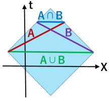
Let us briefly recount the entropic -theorem in the 2d case Casini and Huerta (2004). Consider the entanglement entropy for an interval . We write its Lorentz invariant length as , and then the entropy becomes a function of , which is expressed as . It is also useful to rewrite SSA (1) as
| (2) |
where we regard and in (1) as and , respectively. By taking advantage of the relativistic invariance of 2d QFT, we can choose the subsystems and as in Fig. 1. If we set and , then we find . Thus, SSA (2) leads to the inequality , which implies that is concave as a function of :
| (3) |
The entanglement entropy for 2d CFT vacua is known to take the form , where is the central charge and is the UV cutoff Holzhey et al. (1994). Therefore, we can regard as an effective central charge at the length scale . In this way, the inequality (3) shows the -theorem, which states that the degrees of freedom monotonically decrease under the RG flow.
Even though the -theorem was originally derived using the more traditional field-theoretic method Zamolodchikov (1986), the above SSA argument provides us with a much simpler derivation and shows that at its essence lies the monotonicity of quantum information.
The purpose of this letter is to extend this beautiful and geometrical derivation of the important monotonicity of QFTs, using the entanglement entropy, to cases with boundaries or defects when their bulk theories are conformally invariant.
2. Entropic derivation of the -theorem for BCFTs
Consider a 2d CFT on a 2d Lorentzian flat spacetime, whose coordinates are denoted by and put a time-like boundary at by limiting the spacetime to the right half plane . When the boundary condition at preserves a half of the bulk conformal invariance, this theory is called a boundary conformal field theory (BCFT) Cardy (1984).
It is known that the entanglement entropy for an interval which stretches from the boundary to a point at any time , takes the form Calabrese and Cardy (2004):
| (4) |
where is the UV cutoff and is called the boundary entropy.
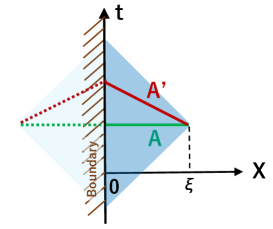
Even if we deform the subsystem (called ) such that it ends on and a boundary point at a time , which is within the domain of dependence of (and its mirror), the entanglement entropy does not change, i.e., . See Fig. 2 for a sketch. This is true for any relativistic field theory with a boundary and is due to the complete reflection at the boundary.
Now, we break the conformal invariance at the boundary by a relevant boundary perturbation . The basic property that the degrees of freedom at the boundary monotonically decrease under the boundary RG flow is known as the -theorem Affleck and Ludwig (1991). The -theorem argues that the boundary entropy in (4) as a function of length scale, so-called the -function, is monotonically decreasing under the boundary RG flow. This theorem was proved by using the boundary RG flow in Friedan and Konechny (2004) and by using the relative entropy in Casini et al. (2016, 2023). For higher dimensional versions of g-functions, refer to Nozaki et al. (2012); Jensen and O’Bannon (2013, 2016); Kobayashi et al. (2019); Casini et al. (2019); Jensen et al. (2019); Goto et al. (2020); Wang (2021); Nishioka and Sato (2021); Wang (2022); Cuomo et al. (2022); Shachar et al. (2023).
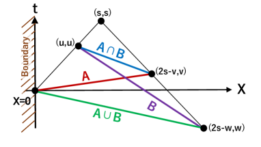
Below, we would like to present another simpler derivation of the -theorem directly from SSA. Consider the Lorentzian setup of Fig. 3 and the implication of SSA:
| (5) |
We write the entanglement entropy for an interval as , whose endpoints are set to be and . When is situated at the boundary , then the entanglement entropy only depends on as we already explained in Fig. 2, and we write this as .
Now we choose the subsystems such that each of the space-like intervals and connects two points on the two null lays which intersect at the point and such that they satisfy , as illustrated in Fig. 3. Then, their entanglement entropies are described by
| (6) |
where we assume and . Below, we appropriately choose the values of and to obtain the tightest bound from SSA.
First, we take the limit , where and become light-like, which is equivalent to the zero width or equally the UV limit. We can understand this by regarding the two point function of twist operators which compute the entanglement entropy as a four point function via the mirror method, which is factoring into a square of two point functions of null separated twist operators. Moreover, this claim is also obvious in the holographic dual of BCFTs Takayanagi (2011); Fujita et al. (2011); Karch and Randall (2001), where the extremal surface dual to is localized near the boundary.
Therefore, in this limit, we can approximate and by their values in the CFT vacuum ignoring the presence of the boundary at :
| (7) |
Thus defined in (5) is evaluated to be
| (8) |
Next, we take the value of very close to by setting , where is an infinitesimally small and positive constant. Then (8) can be rewritten as
| (9) |
Finally, by assuming and taking to be very small such that , we find that the SSA gives the tightest bound:
| (10) |
where takes an arbitrary positive value.
Now we define the entropic -function at the length scale by
| (11) |
such that it gives the boundary entropy at each fixed point following the formula (4). Then SSA (10) leads to the inequality:
| (12) |
This completes the derivation of the entropic -theorem.
3. Entropic -theorem for interface CFTs Next, we extend our previous derivation of the -theorem to interfaces in 2d CFTs. Consider a 2d CFT with central charge on the plane and place an interface along as depicted in Fig. 4. If the interface preserves half of the bulk conformal symmetry, a so-called interface CFT Oshikawa and Affleck (1996); Bachas et al. (2002); Sakai and Satoh (2008), then the entanglement entropy for the interval at any time takes the form
| (13) |
where the constant is the interface entropy. When we consider a relevant perturbation localized on the interface, the entropic -theorem for interface CFTs claims that the entropic g-function
| (14) |
is monotonically decreasing as a function of . Refer to Azeyanagi et al. (2008) for an earlier attempt toward this type of entropic -theorem. Below, we will give a complete derivation from SSA. Refer also to Karch et al. (2023) for an interesting implication from SSA when the interface connects two different CFTs with different central charges.
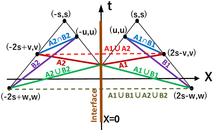
Our argument goes in parallel with our previous one in BCFTs. By doubling the setup of Fig. 2, we choose the subsystems depicted in Fig. 4. We have two copies of the boosted subsystems, each of which is identical to the ones in Fig. 2, named as and . Then we set and in the SSA relation (5). In the limit, this inequality leads to
| (15) |
which is a straightforward extension of (8). As in the BCFT case, we further consider the limit and , and we finally obtain
| (16) |
which is equivalent to the -theorem .
4. Holographic SSA and the Null Energy Condition
The anti-de Sitter/conformal field theory (AdS/CFT) correspondence argues that gravity on a dimensional AdS spacetime is equivalent to a dimensional CFT Maldacena (1998); Gubser et al. (1998); Witten (1998). In AdS/CFT, we can calculate the entanglement entropy in a geometrical way, known as the holographic entanglement entropy (HEE) Ryu and Takayanagi (2006a, b); Hubeny et al. (2007). It is computed from the area of an extremal surface , denoted by , which ends on the boundary of and is homologous to the subsystem in AdS as
| (17) |
where is the Newton constant in the AdS gravity. Interestingly, this HEE allows us to derive SSA in a more geometrical way Headrick and Takayanagi (2007); Wall (2014), which essentially follows from the triangle inequality in classical geometry.
We can extend the AdS/CFT correspondence to the gravity dual of a CFT on a manifold with boundaries by introducing end-of-the-world-branes (EOW branes) Takayanagi (2011); Fujita et al. (2011); Karch and Randall (2001), called the AdS/BCFT correspondence. On the EOW brane, we impose the Neumann boundary condition
| (18) |
where and are the induced metric, extrinsic curvature and matter energy stress tensor on the EOW brane. The HEE in AdS/BCFT is again given by the formula (17) with an important addition that the extremal surface can end on an EOW brane Takayanagi (2011); Fujita et al. (2011). This can be viewed as a change in the homology constraint such that is homologous to relative to the EOW brane.
For a 2d CFT defined on a space with a boundary, its gravity dual is given by a region of 3d AdS (AdS3) surrounded by an EOW brane. Assuming the pure gravity theory in the bulk, we can always choose the metric to be that of the pure AdS3
| (19) |
We specify the profile of EOW brane by such that as in Fig. 5, assuming that it is static. The gravity dual is given by the region . The cutoff of the coordinate is identified with the UV cutoff of the dual CFT. When , the boundary preserves the conformal invariance, i.e., becomes a 2d BCFT. In general, the non-trivial profile of encodes the detailed information of the boundary RG flow (see e.g.Kanda et al. (2023) for an example).
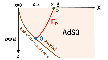
Let us calculate the HEE by using this 3d holographic setup and compare it with our previous arguments for the -theorem. When the subsystem is given by an interval which stretches from the boundary to a point at any time, the HEE is given by
| (20) |
For this, let us calculate the length of the geodesic , which connects between a given point on the AdS boundary and a point on the EOW brane, described by . The value of is fixed by minimizing as a function of . Notice that since the EOW brane is static, is on a constant time slice, leading to in Fig. 2.
Since the geodesic is orthogonal to the EOW brane at and is given by a part of a circle in plane, we find the relation between and :
| (21) |
and the length of the geodesic is computed as
| (22) |
For example, if we set , then we find
| (23) |
which leads to the standard form of the EE (4) in 2d BCFT.
For a generic profile , we obtain:
| (24) |
The non-negativity of this quantity is equivalent to the SSA condition (10).
Indeed, we can find that (24) is non-negative if we assume the null energy condition, i.e., for any null vector in AdS3.
The null energy condition on the EOW brane leads to the condition as shown in Takayanagi (2011); Fujita et al. (2011), where a holographic -theorem was derived.
This allows us to guarantee .
This is found as follows:
First, in the UV limit , we expect the boundary to become conformal, which means , leading to at .
Moreover, the derivative is non-positive due to the null energy condition.
Thus, these manifestly show .
In this way, SSA in the setup of Fig. 1 precisely requires that the classical gravity satisfies the null energy condition in the gravity dual.
5. Holographic SSA in Static Backgrounds
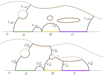
In the above calculations of SSA, it was crucial that we considered the Lorentzian setup taking advantage of boost operations in relativistic QFTs. On the other hand, if we assume all subsystems () and the dual extremal surfaces () are on the same time slice , then we can show that the HEE in AdS/BCFT always satisfies SSA for any profile of the EOW brane at (see also Chou et al. (2021); Chang et al. (2018) for earlier confirmation of SSA in particular examples). More generally, this claim can also be applied to a setup with a time reversal symmetry . Note that this does not contradict the null energy condition because we can compensate for the arbitrary shape of the EOW brane at the specific time by choosing an appropriate time evolution of the EOW brane profile such that the null energy condition is maintained.
Since the essence of this argument does not depend on the dimension, we will continue to focus on the specific example of AdSBCFT2. Let be an interval, whose endpoints are given by and , its HEE is computed as the minimum of the area of two configurations of surfaces:
| (25) |
where is the disconnected HEE (20) and is the connected HEE given by
With these preparations, we can prove SSA for AdS3/BCFT2 on a time slice which has the time reversal symmetry. We take three subsystems , , and on . Recalling that the entanglement wedge preserves the order of inclusion, we have
| (26) |
where denotes the homology region which is the entanglement wedge of projected onto . This leads to the implication that the intersection is non-empty. Therefore, the extremal surface of subsystem can be divided into three parts:
| (27) |
The first one denotes the part containing , i.e. and the second one is the outer part. The last one is the common part . and are defined similarly. Furthermore, for subsystem , denotes the parts of the EOW brane which enclose . Namely, by the homology condition on the homology region, we have
| (28) |
We define as the intersection , then satisfies the homology condition:
| (29) |
Because of the extremality of , we must have
| (30) |
Furthermore, also satisfies the homology condition
| (31) |
thus we have
| (32) |
Finally, by adding the two inequalities (30) and (32), we have
| (33) | ||||
| (34) | ||||
| (35) |
Therefore, SSA on holds.
It is also possible to show that the monogamy of mutual information (MMI) Hayden et al. (2013) holds for the same setup of AdS/BCFT at a time slice. MMI states that for any choice of subsystems, the following inequality holds:
| (36) |
MMI has been shown to hold in AdS/CFT setups without EOW branes in Hayden et al. (2013).
Appendix A provides the details of the proof of MMI in the case of static AdS/BCFT using similar arguments to that of SSA.
Acknowledgements
We are very grateful to Horacio Casini for valuable comments on the draft of this article. We also thank Isaac Kim, Yuya Kusuki and Masamichi Miyaji for useful discussions. This work is supported by MEXT KAKENHI Grant-in-Aid for Transformative Research Areas (A) through the “Extreme Universe” collaboration: Grant Number 21H05187. TT is also supported by Inamori Research Institute for Science and World Premier International Research Center Initiative (WPI Initiative) from the Japan Ministry of Education, Culture, Sports, Science and Technology (MEXT), by JSPS Grant-in-Aid for Scientific Research (A) No. 21H04469.
Appendix A Appendix A: SSA and MMI in AdS/BCFT
In this section, we show that SSA and MMI on a time slice hold for any static setups of AdS3/BCFT2.SSA states that for any three intervals , and on a time slice, the following inequality holds,
| (37) |
The tripartite mutual information,
| (38) |
can be either positive or negative in general quantum systems. MMI states that holds for any choice of subsystems.
We consider a set consisting of three intervals on a time slice with an EOW brane . The holographic entanglement entropy of a subsystem is given by the area of the corresponding extremal surface in the bulk spacetime,
| (39) |
where is the Newton’s constant. The extremal surface and the EOW brane surface are taken so that is homologous to the subsystem . In other words, there exists a corresponding homology region such that it is enclosed as
| (40) |
Recalling that the entanglement wedge preserves the order of inclusion, we have the following relations,
| (41) |
This implies that the intersection is non-empty. By cyclic permutation of , and , we also have the similar relations for the intersection and . Therefore, the extremal surface is divided into four parts,
| (42) |
where
| (43) | ||||
| (44) | ||||
| (45) | ||||
| (46) |
Similarly, we define and for by cyclic permutations of , and . We also define and for in the same manner.
A.1 Proof of SSA on a time slice
The bulk region satisfies the homology condition with respect to , where we define
| (47) | ||||
| (48) |
By the extremality of , we have the condition
| (49) |
the area of is minimized among all the surfaces homologous to .
The bulk region satisfies the homology condition with respect to , where we define
| (50) | ||||
| (51) |
By the extremality of , we have the condition
| (52) |
Thus, we have
| (53) |
which implies the SSA.
A.2 Proof of MMI on a time slice
The bulk region satisfies the homology condition with respect to , where we define
| (54) | ||||
| (55) |
By the extremality of , we have the condition
| (56) |
We obtain the similar condition for and as
| (57) | ||||
| (58) |
by cyclic permutations of , and .
The bulk region satisfies the homology condition with respect to , where we define
| (59) | ||||
| (60) |
By the extremality of , we have the condition
| (61) |
Thus, we have
| (62) |
which implies the MMI.
References
- Lieb and Ruskai (1973a) E. H. Lieb and M. B. Ruskai, J. Math. Phys. 14, 1938 (1973a).
- Lieb and Ruskai (1973b) E. H. Lieb and M. B. Ruskai, Phys. Rev. Lett. 30, 434 (1973b).
- Casini and Huerta (2004) H. Casini and M. Huerta, Phys. Lett. B 600, 142 (2004), arXiv:hep-th/0405111 .
- Casini and Huerta (2012) H. Casini and M. Huerta, Phys. Rev. D 85, 125016 (2012), arXiv:1202.5650 [hep-th] .
- Casini et al. (2017) H. Casini, E. Testé, and G. Torroba, Phys. Rev. Lett. 118, 261602 (2017), arXiv:1704.01870 [hep-th] .
- Holzhey et al. (1994) C. Holzhey, F. Larsen, and F. Wilczek, Nucl. Phys. B 424, 443 (1994), arXiv:hep-th/9403108 .
- Zamolodchikov (1986) A. B. Zamolodchikov, JETP Lett. 43, 730 (1986).
- Cardy (1984) J. L. Cardy, Nucl. Phys. B 240, 514 (1984).
- Calabrese and Cardy (2004) P. Calabrese and J. L. Cardy, J. Stat. Mech. 0406, P06002 (2004), arXiv:hep-th/0405152 .
- Affleck and Ludwig (1991) I. Affleck and A. W. W. Ludwig, Phys. Rev. Lett. 67, 161 (1991).
- Friedan and Konechny (2004) D. Friedan and A. Konechny, Phys. Rev. Lett. 93, 030402 (2004), arXiv:hep-th/0312197 .
- Casini et al. (2016) H. Casini, I. Salazar Landea, and G. Torroba, JHEP 10, 140 (2016), arXiv:1607.00390 [hep-th] .
- Casini et al. (2023) H. Casini, I. Salazar Landea, and G. Torroba, Phys. Rev. Lett. 130, 111603 (2023), arXiv:2212.10575 [hep-th] .
- Nozaki et al. (2012) M. Nozaki, T. Takayanagi, and T. Ugajin, JHEP 06, 066 (2012), arXiv:1205.1573 [hep-th] .
- Jensen and O’Bannon (2013) K. Jensen and A. O’Bannon, Phys. Rev. D 88, 106006 (2013), arXiv:1309.4523 [hep-th] .
- Jensen and O’Bannon (2016) K. Jensen and A. O’Bannon, Phys. Rev. Lett. 116, 091601 (2016), arXiv:1509.02160 [hep-th] .
- Kobayashi et al. (2019) N. Kobayashi, T. Nishioka, Y. Sato, and K. Watanabe, JHEP 01, 039 (2019), arXiv:1810.06995 [hep-th] .
- Casini et al. (2019) H. Casini, I. Salazar Landea, and G. Torroba, JHEP 04, 166 (2019), arXiv:1812.08183 [hep-th] .
- Jensen et al. (2019) K. Jensen, A. O’Bannon, B. Robinson, and R. Rodgers, Phys. Rev. Lett. 122, 241602 (2019), arXiv:1812.08745 [hep-th] .
- Goto et al. (2020) K. Goto, L. Nagano, T. Nishioka, and T. Okuda, JHEP 08, 048 (2020), arXiv:2005.10833 [hep-th] .
- Wang (2021) Y. Wang, JHEP 11, 122 (2021), arXiv:2012.06574 [hep-th] .
- Nishioka and Sato (2021) T. Nishioka and Y. Sato, JHEP 05, 074 (2021), arXiv:2101.02399 [hep-th] .
- Wang (2022) Y. Wang, JHEP 02, 061 (2022), arXiv:2101.12648 [hep-th] .
- Cuomo et al. (2022) G. Cuomo, Z. Komargodski, and A. Raviv-Moshe, Phys. Rev. Lett. 128, 021603 (2022), arXiv:2108.01117 [hep-th] .
- Shachar et al. (2023) T. Shachar, R. Sinha, and M. Smolkin, SciPost Phys. 15, 240 (2023), arXiv:2212.08081 [hep-th] .
- Takayanagi (2011) T. Takayanagi, Phys. Rev. Lett. 107, 101602 (2011), arXiv:1105.5165 [hep-th] .
- Fujita et al. (2011) M. Fujita, T. Takayanagi, and E. Tonni, JHEP 11, 043 (2011), arXiv:1108.5152 [hep-th] .
- Karch and Randall (2001) A. Karch and L. Randall, JHEP 06, 063 (2001), arXiv:hep-th/0105132 .
- Oshikawa and Affleck (1996) M. Oshikawa and I. Affleck, Phys. Rev. Lett. 77, 2604 (1996), arXiv:hep-th/9606177 .
- Bachas et al. (2002) C. Bachas, J. de Boer, R. Dijkgraaf, and H. Ooguri, JHEP 06, 027 (2002), arXiv:hep-th/0111210 .
- Sakai and Satoh (2008) K. Sakai and Y. Satoh, JHEP 12, 001 (2008), arXiv:0809.4548 [hep-th] .
- Azeyanagi et al. (2008) T. Azeyanagi, A. Karch, T. Takayanagi, and E. G. Thompson, JHEP 03, 054 (2008), arXiv:0712.1850 [hep-th] .
- Karch et al. (2023) A. Karch, Y. Kusuki, H. Ooguri, H.-Y. Sun, and M. Wang, JHEP 11, 126 (2023), arXiv:2308.05436 [hep-th] .
- Maldacena (1998) J. M. Maldacena, Adv. Theor. Math. Phys. 2, 231 (1998), arXiv:hep-th/9711200 .
- Gubser et al. (1998) S. S. Gubser, I. R. Klebanov, and A. M. Polyakov, Phys. Lett. B 428, 105 (1998), arXiv:hep-th/9802109 .
- Witten (1998) E. Witten, Adv. Theor. Math. Phys. 2, 253 (1998), arXiv:hep-th/9802150 .
- Ryu and Takayanagi (2006a) S. Ryu and T. Takayanagi, Phys. Rev. Lett. 96, 181602 (2006a), arXiv:hep-th/0603001 .
- Ryu and Takayanagi (2006b) S. Ryu and T. Takayanagi, JHEP 08, 045 (2006b), arXiv:hep-th/0605073 .
- Hubeny et al. (2007) V. E. Hubeny, M. Rangamani, and T. Takayanagi, JHEP 07, 062 (2007), arXiv:0705.0016 [hep-th] .
- Headrick and Takayanagi (2007) M. Headrick and T. Takayanagi, Phys. Rev. D 76, 106013 (2007), arXiv:0704.3719 [hep-th] .
- Wall (2014) A. C. Wall, Class. Quant. Grav. 31, 225007 (2014), arXiv:1211.3494 [hep-th] .
- Kanda et al. (2023) H. Kanda, M. Sato, Y.-k. Suzuki, T. Takayanagi, and Z. Wei, JHEP 03, 105 (2023), arXiv:2302.03895 [hep-th] .
- Chou et al. (2021) C.-J. Chou, B.-H. Lin, B. Wang, and Y. Yang, JHEP 02, 154 (2021), arXiv:2011.02790 [hep-th] .
- Chang et al. (2018) E.-J. Chang, C.-J. Chou, and Y. Yang, Phys. Rev. D 98, 106016 (2018), arXiv:1805.06117 [hep-th] .
- Hayden et al. (2013) P. Hayden, M. Headrick, and A. Maloney, Phys. Rev. D 87, 046003 (2013), arXiv:1107.2940 [hep-th] .