We define the notion of stochastic stability, already present in the
literature in the context of smooth dynamical systems, for invariant
measures of cellular automata perturbed by a random noise, and the
notion of strongly stochastically stable cellular automaton. We study
these notions on basic examples (nilpotent cellular automata, spreading
symbols) using different methods inspired by those presented in [16].
We then show that this notion of stability is not trivial by proving
that a Turing machine cannot decide if a given invariant measure of
a cellular automaton is stable under a uniform perturbation.
Mathieu Sablik was partially supported by ANR project Difference (ANR-20-CE48-0002) and the project Computability of asymptotic properties of dynamical systems from CIMI Labex (ANR-11-LABX-0040).
1. Introduction
1.1. Stochastic stability: physics motivation
Dynamical systems, like cellular automata, are models for physical
observations. They can be studied as deterministic models, despite
the presence of errors compared to the real phenomenon: model errors,
measures errors, small perturbation, etc. The study of stochastic
stability (or zero-noise limit) aim to determine on the behaviors
encountered in those deterministic models, which one are resistant
to noise, and thus can be thought of as having a physical “sense”.
More precisely, let us define a discrete dynamical system
with a compact metric system and a continuous map.
The long-term behavior can be described by their invariant measures:
denote one of them by . To decide which ones had physical
meaning, A. N. Kolmogorov proposed the following tool [3]:
suppose a family of dynamics
obtained by perturbation of by a noise of size . For
each, denote by a -invariant measure.
If (in some sense), then
is said to be stochastically stable (or statistically
stable) under small perturbation.
This question is the subject of lot of articles in the context of
smooth dynamical systems, where is a Riemannian manifold and
have some regularity properties (or not), and the measures considered
are often continuous with respect to the Lebesgue measure [3, 23].
Further works even studied the regularity properties at of the
map and their link to the speed of convergence
(the linear response [1] or even quadratic response [10]).
Cellular automata (CA) were first introduced by Von Neumann at the
end of the 40’s to model local interactions phenomenons [18].
A cellular automaton can be defined as a dynamical system defined
by a local rule which acts synchronously and uniformly on the configuration
space where is a finite alphabet. These simple
models have a wide variety of different dynamical behaviors and they
are used to model physical systems defined by local rules but also
models of massively parallel computers.
Their perturbed counterpart, Probabilistic Cellular Automata (PCA)
are studied to understand the robustness of their computation, in
particular their dependence towards the initial condition. When a
PCA is ergodic, in the sense that every trajectory converges
to the same distribution, it forgets its initial condition, and thus
no reliable computation is possible. PCA are generally ergodic and
in [16] the authors exhibit large classes of cellular automata
which have this behavior. There exists some examples of non ergodic
CA in dimension 2 and higher [22]. In dimension 1 non ergodic
CA are more complex [8] and their construction is based
on fault-tolerant model of computation.
If this problem of fault-tolerant models comes from theoretical computer
science, it could also have practical application. The perturbation
of a cellular automaton can be thought of as errors that can occur
in the update of a computer bit. If such errors are really rare in
our daily computers, they are (theoretically) more frequent in computers
aboard spacecrafts, as they are more vulnerable to cosmic neutron
rays [14]. In this paper the errors will occur with probability
.
1.3. Stochastic stability for cellular automata
It is natural to try to understand the effect of small random perturbations
on the dynamics of cellular automata and more precisely if the behavior
of the deterministic model can be observed despite the presence of
small errors. As models of computation, they can be used to study
the reliability of computation against noise.
Since a large classes of cellular automata are ergodic, we don’t need
the help of other assumptions (like SRB measures) to have the uniqueness
of the invariant measure for each perturbed PCA, which allows us to
study the limit(s) of a family of measures
when goes to zero. We can hope that this behavior select
only a few of the invariant measures of the deterministic CA, as they
are much more inclined to have a lot of invariant measures. If the
CA is not ergodic, we consider stable measures as the set of adherence
values when goes to of invariant measures of the
perturbed system.
This notion of stability is quite similar to the stability of trajectories
studied in [9]. In this article the authors characterize
monotonic cellular automata such that the orbit of the trajectory
of the uniform configuration with the symbol stays near this
configuration when the perturbation parameter goes to 0. When the
cellular automata is ergodic, this notion implies the previous notion
of stochastic stability for the Dirac mass on the configuration with
only s. Another notion of stability also appears in [5]
to study how a probabilistic cellular automaton can correct mistakes
of some tilings defined by local rules.
The first examples of CA that would seem stable are classes of CA
which converges rapidly to a fixed point: we take the example of nilpotent
CA. Another interesting case would be classes of CA with several fixed
points, but that all but one could be described as “unstable”.
Here, we take the example of CA where a symbol is spreading, and verify
that the stochastic stability only select the “stable” point (with
no necessary the monotonic assumption as in [5]). If the
notion of stochastic stability is intuitive, proving that a particular
CA is stable may not be. In fact, we prove that it is an undecidable
property; we can draw parallel to other “basic” properties that
are in fact undecidable for CA, like nilpotency [15].
1.4. Description of the paper
In section 2 we recall the basic tools for the study of cellular automata,
and define the ones for the study of their stochastic stability nature.
In section 3 and 4, we apply this notion on simple examples where
we expect stability to appear: nilpotent CA and CA with a spreading
symbol. The stable measure for those automata is very simple, as it
is the Dirac mass on a uniform configuration. Beside proving the stability
of this measure, we also show different approaches to obtain an upper
bound on the speed of convergence towards it.
The two final sections are independent of the two previous ones. In
section 5 we present proofs for computation results we use in the
following section. Those results are Proposition 5.1
and 5.2, which gives an asymptotic development
for several functions when the noise goes to zero.Finally, in section 6 we prove that given a CA perturbed by a standard
noise, the stochastic stability of a measure is undecidable, as stated
in Theorem 6.1. To prove this theorem, we simulate
a Turing machine in a construction already described in [2]
and [4].
2. Stochastic stability for cellular automata
Let be a finite alphabet of symbols, and define
the space of configurations of endowed with the product
topology. An application is a cellular automaton (CA)
if there is a finite neighborhood
and a local rule such that for all ,
where .
A transition kernel is a probabilistic cellular automaton
(PCA) if there is a finite neighborhood
and a stochastic matrix (local rule)
such that for all , .
Moreover, it is a -perturbation of a CA if they are
defined on the same alphabet, have the same neighborhood, and if their
local rules and verify for all ,
Deterministic and probabilistic cellular automata both acts on
the set of Borel probability measures on , by
for any PCA, and observable. A measure
is -invariant if . Recall that
is compact and metrizable for the weak convergence topology:
if for all cylinders
.
Definition 2.1(Stochastic stability of a measure).
A measure is stochastically stable under
if there exists a numerical sequence
converging towards and a sequence
verifying:
(1)
is -invariant.
(2)
.
Definition 2.2(Strong stochastic stability of a cellular automaton).
A cellular automaton is strongly stochastically stable
under if it admits only
one stochastically stable measure.
Observe that by definition of an -perturbation and continuity
of the action of on , all stochastically
stable measures are invariant measure for .
In order to compare speeds of convergence, we use the total variation
distance on a finite observation window: for a finite set
and two measures , define
. If is a sequence of , the following
equivalence holds:
Finally, for a symbol , we denote by the configuration
such that for all . The
Dirac mass concentrated on this configuration will be denoted by .
3. Nilpotent CA
The first class of CA we can study is the nilpotent ones. A cellular
automaton is said to be nilpotent if there is a integer
such that is a constant function. By shift-invariance
a nilpotent CA admits a symbol, which we will denote by ,
such that is the constant function equals to .
As they only admit as an invariant measure, it is immediate
that it is also stochastically stable. The authors of [16]
prove that for small perturbations, ergodicity is conserved. We can
reuse the same kind of arguments to prove an upper bound on the speed
of convergence on a finite window of observation.
Theorem 3.1(Stability for nilpotent CA).
Let
a family of -perturbations of a nilpotent CA on .
For small enough, we denote by the unique
invariant measure of . Then there is a constant
such that for all finite ,
Proof.
Denote by the cylinder .
One easily gets
Using [16]’s notations, we denote by the
neighborhood of the CA , and
(with ). By definition of an -perturbation,
one has
(i.e. there is no mistake in each cell of ). By iterating it,
one gets
(i.e. for each points of , there is no mistake in its neighborhood
for the last iterations, i.e. on the points inside the dotted
area on Figure 3.1).
Figure 3.1. Proof of theorem 3.1. To
have a at , it suffices to not make any mistake on the
cells inside the grayed area.
By -invariance, one gets
and then our result with (independent
of ).
∎
4. Spreading CA
A cellular automaton admits as a spreading state
if it verifies for all one has:
Example 4.1.
The CA defined on
admits as a spreading state.
Contrary to a nilpotent CA, such an automaton can have several fixed
points: in particular, is not necessarily the only invariant
measure. However, it is very intuitive to think that, as long as they
can appear, the will spread on the grid, and the measure we can
observe are thus near . For that reason, we consider
perturbations that are -positive: for any ,
.
If is endowed with an order (e.g. ),
such CA can be thought as having similar properties as monotonous
eroders, as defined and studied in [21, 9]. In those
articles, the author studied the stability of the trajectory beginning
at . The monotonous eroders CA having this trajectory
stable are called stable. It is easy to prove that, if generalizing
this definition of stability to all CA, a stable CA which is ergodic
when perturbed admits as its unique stochastically stable
measure.
We present two different approaches for different cases: in the first
one, we prove the stochastic stability of under any
-positive perturbation for 1-dimensional CA admitting as
a spreading state. As we do not only consider monotonous CA, this
is not an application of [9]. In the second one, we prove
the stability for any dimension, but only for a binary alphabet
and a more restrictive class of noise. Here, all spreading CA on a
binary alphabet are monotonous, and thus the stability of
is a consequence of the results in [21]. However, the proof
we propose is based on the computations of [16], which also
provide a speed of convergence in certain cases.
4.1. 1-dimensional
In this part, we only consider 1-dimensional CA, i.e. defined on .
Theorem 4.2.
Let be a CA on with
neighborhood an interval of with length
admitting as a spreading state, and
a family of -positive -perturbations. For all ,
let . Then for all finite interval
, there is a constant such that
4.1.1. Spread graph
The following paragraph is adapted from the ideas one can read in
more details in [22] and [6]. Let us describe what
is a spread graph.We construct it in three
steps, illustrated in Figure 4.1:
(1)
Consider the (infinite) dependency graph of the cell , at position
and time , for a CA with neighborhood ,
tilted to keep symmetry.
(2)
In order to use tools for planar graph, each step of the CA is decomposed
into steps of a CA with neighborhood .
Its definition does not matter as we are only considering the spread
of the symbol .
(3)
To represent the noise, each vertex corresponding to a “true cell”
at time and position is split into two vertices,
linked with an edge . They are always open in the down
direction, but are only open in the up direction with a probability
greater than , when there is no error in the cell
at time .
Figure 4.1. Left: step 1, the first three levels
of the initial dependency graph for .
Center: step 2, the decomposition into a planar graph.
Right: step 3, adding the noise.
Definition 4.3.
The spread graph associated to ,
a collection of independent uniform variables on ,
is the spread graph where the edge is open in the up
direction when .
The tilted edges, that represent the spread of the symbol by
the deterministic cellular automaton, are always open in the up
direction and closed in the down direction. What is the probability
to have a infinite open path ending the top vertex ? To answer
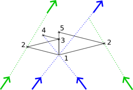
it, consider the dual of this planar graph as in figure 4.2
Figure 4.2. Left: The first three levels of the original
graph. Right: the first three levels of the the dual graph. Note that
the outer vertices actually represent the same region of the original
graph.
(for a complete definition see [6]). Each edge has a
dual edge . For each direction of , the corresponding
direction on is the direction from left to right when
we go along in the given direction. Every edge
is open in a direction if and only if is closed in the corresponding
direction. For our graph, the following table gives the results.
There is an (infinite) open path ending in if and only if there
is no open self-avoiding contour in the dual graph leaving on
the left.
Corollary 4.5.
The probability to have an infinite path ending in is greater
than .
Proof.
Let us bound the probability of existence of an open self-avoiding
contour in the dual graph. We can suppose that every contour begins
and finishes at the top cell of the dual graph. The probability that
there is such a contour is less than
where is the number of contours going through horizontal
arrows. As a contour goes through
an equal number of, and
, a contour is of length . As there is at most
choices of direction at each point of the dual graph, a contour can
be associated to a unique function from
to . Thus, ,
and the probability that such a contour exists is less than .
Thus, the probability to have an open path ending in is greater
than .
∎
4.1.2. Update functions
To prove the theorem, we need an ergodicity property of this kind
of CA.
Definition 4.6.
An update function for the local rule
is a function such that for any and ,
.
A global update map is defined as
. To simulate
the PCA, we can recursively define
by ,
and give ourselves independent
random variables uniformly distributed over .
Proposition 4.7([16], Theorem 3.11 and Proposition 3.3).
Let be a CA admitting as a spreading symbol. Then there
is an such that ,
every -positive -perturbation of is uniformly
ergodic. Moreover, there is a defined uniquely by the
such that is almost surely
constant, with .
Observe that in order to have ,
it suffices to have in the spread graph defined by
an open path which end at the top vertex and begin at least in
the level : the symbol from this level will spread towards
the top via this open path.
Without loss of generality, we can suppose that the neighborhood
is . We denote
by the unique measure of . As in
the proof for the nilpotent case, the total variation distance to
a Dirac distribution is .
For any , define ,
such that
and .
By definition of an -perturbation, we have .
By iterating the last inequality, we obtain
where ,
which corresponds to the number of cells where it suffices to not
have any mistake to be sure to have only the symbol in all the
cells of at (see Figure 4.3) . For ,
we have .
Figure 4.3. Proof of theorem 4.2.
To have a when on all , it suffices to have one in
and not make any mistakes on
the cells of the colored area. Time goes upward.
By the previous propositions is constant.
One can then only use its value on the entry .
where the final inequality is by percolation.
∎
Example 4.8.
For the simple case , the result
is
The spread graph used in the proof is much simpler (Figure 4.4),
and is the one described in [22].
Figure 4.4. Illustration for neighborhood .
In blue the spread graph, in black the dual graph. Vertical red arrows
have a probability to be “closed”,
and thus the horizontal dashed red ones have a probability
to be “open”.
4.2. -dimensional binary
For , we define such that : the symbol is spreading. We will prove the stochastic stability
of using Fourier analysis. In [16], the authors
prove that a perturbation of by a zero-range noise is (under
certain circumstances) ergodic.
Theorem 4.9.
Let defined as above, and
a zero-range perturbation of , with noise matrix such that , and .
Let be the unique -invariant measure
(for ). Then for all finite ,
In particular, is stochastically stable if .
Remark 4.10.
The condition implies a -positive perturbation,
so we already know that is stochastically stable if
we are in the case , with a speed of convergence that is at
least linear. Depending on the value of
and the ratio ,
the conclusion may be stronger or weaker than the previous theorem.
In fact, in the case ,
this theorem tells nothing on the stochastic stability of :
as mentioned in the beginning of the section, we know that
is stochastically stable as a direct consequence of the stable eroder
nature of the CA (as proven in [21]) and the uniform ergodicity
of its perturbation (as proven in [16]).
To prove this theorem, we use the Möbius basis of .
Definition 4.11.
Let be defined by , . For
a finite , let be defined by
The set of all for finite forms a basis of .
For any observable , we note its decomposition on
this basis as . We finally
define a semi-norm associated to it,
As and ,
the measure is well-defined and
is uniformly ergodic: in particular for all probability measure
on , . By
linearity,
and by proposition 4.12, one deduces
that
for , and .
Also, .
Then, with , one gets
And so
Taking the limit,
and thus .
In the case ,
.
Therefore,
∎
Example 4.13.
For a uniform noise, i.e. where ,
one gets a speed of convergence in ,
therefore a linear speed again for .
5. Computational lemmas
This section is dedicated to the proof of the two following results,
Proposition 5.1 and 5.2.
We will use them in the last section of the article to prove the undecidability
of stochastic stability. The proofs are purely computational, and
don’t give much insight on the main theorem.
Proposition 5.1.
For all and ,
the following holds:
where is the gamma function defined by .
Proposition 5.2.
Let and be such
that . Then,
Both results are consequence of the following classical lemma and
its corollary, which proofs are in Appendix A.
Lemma 5.3.
Let and
be such that and are power series
with convergence radius greater or equal to , and
diverges. If , then
Corollary 5.4.
Define and .
If , then
By direct induction, one can generalize to the case ,
etc.
Consider first the case . Standard calculations (see for
example [7, chapter VI.2]) gives
The Stirling formula
leads us to define ,
which verifies
and the hypotheses of Lemma 5.3. Thus, .
For the general case , define .
Using the previous case, .
Define and , and their respective cumulative sums and . By integral-sums
comparison, one has
and
The previous corollary gives the wanted result.
∎
For the second proposition, the idea is to split the sum in two, and
use the lemma to produce a asymptotic development for each.
Lemma 5.5.
One has the following asymptotic development:
Proof.
Denote by and by Their respective cumulative sums are denoted by
and . Consider then the following radius-1
power series:
and .
Finally, define .
By Lemma 5.3, it suffices to prove that .
Indeed, it follows that ,
and thus .
(1)
Computations shows that
and .
(2)
Because for ,
we have
and
The result is the same if adding until as .
(3)
Using Stirling formula, .
Series-integral comparison gives .
If we define as , one
has . By adding the comparison
relations, it follows that .
Thus .
Moreover,
Addding the comparison relations
Combining the two results yields
(4)
Thus,
(5)
Decompose every as with
and . One gets
In one hand, .
In the other hand, as and
are non-decreasing one gets
So
and finally .
∎
Corollary 5.6.
For , one has the following asymptotic
development:
Proof.
By .
∎
Define for fixed , , as . One can verify that the condition is enough to have
well-defined.
Lemma 5.7.
For , such that
, one has the following asymptotic development:
Proof.
The proof is similar to the previous one, with
and . Define similarly and .
(1)
Computations leads to .
By , one obtains .
(2)
Computations leads to
(3)
Similarly,
(4)
Thus,
(5)
With the decomposition where ,
it suffices to observe that
where . By Corollary 5.6 and Lemma 5.7,
one can obtain their respective asymptotic development. Using them
both leads to
∎
6. Undecidability
The purpose of this section is to show that given a cellular automaton, it is undecidable to know if it is strongly stochastically stable. Thus we cannot hope to have a simple characterization of this phenomenon.
Theorem 6.1.
For and a CA, denote
by its perturbation by a uniform noise of scale .
The problem which take in input the rule of a cellular automaton and say that is stochastically stable under is undecidable.
To prove the theorem, we simulate a Turing machine in the CA such
that the wins if and only if the machine halts. The construction
is heavily inspired by the one described in [2, section 3]
and [4, section 5]. In short, a special symbol is used
to initialize the machine, and create a cone where the calculations
occur, protected from outside s. If the machine halts, it create
a inside the cone that quickly erase the latter.
The main idea behind the construction is that if the machine halts,
the cones disappear in a finite amount of time so the “should
win”. If the machine does not halt, the cones are infinite and stops
the . The errors are both useful and a problem: they are the one
that make the symbols appear in the first place, but can perturb
the computation of the machine.
In this section, we first recall some basic notions about Turing machines,
and then describe with more details the CA and its perturbation. The
last parts deals with the two cases, when the Turing machine halts
in a finite amount of time or not.
6.1. Definition of a Turing machine
For a recent broader study on the subject of Turing machines and its
applications, see for example [17, 20].A Turing machine is one of many computation model. Consider a bi-infinite
tape (indexed by ) where on each cell is inscribed a symbol ,
where is a finite alphabet. Denote by a finite
set of state of the head of the machine, containing a
halting state and an initial state. Finally, define by
the transition function of the machine. The Turing machine in itself
is the tuple .
Initially, the head is positioned at the cell indexed by in the
state , while each cell of the tape is inscribed with the
empty symbol . At each step, the head with state
read the symbol on the cell it is on, then follows the instruction
of the transition function :
the head takes the state , replace by
on the cell it is on, and take a step in the direction given by .
and being finite and each step following a local rule,
one can easily simulate the run of a Turing machine in a cellular
automata. In our case, it is the role of the symbol which create,
after one iteration of the CA, a zone bounded by two walls containing
the representation of the empty tape and one symbol
at the same position occupied
previously by representing the head of the Turing machine. The
walls move at speed in each direction, leaving
on their way: in the absence of errors, the head moving at most at
speed 1 in a direction cannot meet a wall, and thus its run is not
affected by the finite nature of the tape.
Turing machines are the base tool to prove undecidability problems,
as the problem “the machine reach the state in a finite
amount of steps” is undecidable (or uncomputable): there is no algorithm
such that, given , can determine
if this machine halts in a finite amount of time.
6.2. Description of the CA
6.2.1. General description
In the construction of [2], the maximum speed was ,
and the particles had speed and . In
order to simplify the proof (e.g. the particles have integer speeds),
we choose the maximal speed to be . The neighborhood radius
will then be also . The alphabet of cardinal
is composed of the following symbols:
•
, which are spreading on the at speed , but also on the
walls (if on the right side).
•
, the tape on which the Turing machine is running. One can decompose
it in a finite number of , where
where if ,
is the symbol written on the tape while is the state
of the head of the Turing machine which is positioned here. Otherwise
when it is just the symbol written
on the tape. Finally is the set encapsulating the signals
used for the comparison: comparison signals , the destruction
signals and the position signal. If the state is
reached (when the machines halts), the symbol is replaced by a ,
which will spread on the tape around it.
•
, which initializes the Turing machine and create walls on each
side.
•
Walls: the left and right inner walls with speed ,
and the outer left and right walls with speed .
They stop the propagation of the , but only in one direction;
they are erased if caught up by a from the other direction. If
the walls are created by a cell, the space between them is filled
with .
Figure 6.1. Illustration of the behavior of the CA.
Remark 6.2.
In the following we consider that
the only fixed point of is (and thus
is the only -invariant Dirac mass). In the case that there is
a type of symbol such that is a fixed point, we
can define a new symbol with the same behavior under
the CA, but with the added rule that
and .
6.2.2. Collisions
The motivation behind taking this construction instead of a simpler
one is that in the absence of perturbation, a cone created
by a symbol can’t be erased. This external robustness is granted
by the double layer of walls each side of the cone and signals such
that, if two cones collides, only the youngest one (i.e. created by
the most recent ) survives.
Figure 6.2. Illustration of the collision process.
The collision is handled as illustrated in the space-time diagram
in Figure 6.2:
(1)
When two outer walls collides, they produce a vertical position signal,
as well as two comparison signals propagating trough the buffer zones.
(2)
They collide to their respective inner wall.
(3)
The comparison signal bouncing off the younger inner wall arrives
first to the position signal: a destruction signal is sent.
(4)
The destruction signal erases the older outer wall.
(5)
The other comparison signal is destroyed upon arrival, letting the
younger outer wall erasing the information in the older cone.
All the comparison and destruction signals propagate at speed
trough the buffer zones, to ensure that the older outer walls are
erased before encountering the younger inner wall.
6.2.3. Perturbation
At each step of the automaton, the configuration is perturbed by a
uniform noise of size : independently from each other,
each cell has a probability to have its symbol replaced
by a symbol chosen uniformly in . The local rule is then
To make computations clearer, we define
independent random variables such that for all ,
and It defines a local rule
with , which can be made in a global rule
via .
It is not difficult to see that for all observable , .
Thus, for a -invariant measure , we
can define a stationary sequence which
verifies for all the relation
and is distributed according to . The event
is realized when an error is made at time
in cell , and a symbol is written instead of the expected
result of the CA.
Remark that because it only appear via errors, for each -invariant
measure the probability to have a symbol in a given cell is ;
and by independence of the errors (i.e. the independence of ),
the probability to have at least one symbol over cells is
.
6.3. Case where the TM doesn’t halt
Suppose that the Turing doesn’t halt: let us show that for any collection
of -invariant
measures, the value
does not converge towards 1 when goes to . Here, we
will prove that there is a map such that
and .
A produces a zone of slope at least of
symbols. Thus, in order to have a , it suffices that step
before there was a symbol within the
cells, and that there wasn’t any error on the dependence cone of our
original cell over the last steps. The size of that cone is .
See Figure 6.3.
Figure 6.3. Case where the TM doesn’t halt. If there is no
error in the grayed area and a symbol in the blue area, there
must be a at .
The being only able to appear via an error, these events are
disjoints for distinct , thus
Suppose that the Turing machine halts after a finite amount of steps:
let us show that for any collection
of -invariant measures, the value
converges towards 1 when goes to . Here, we will prove
that there that the probability to encounter any other symbol goes
to .
6.4.1. Definitions
When the machine halts (in a finite time), the heads become a
which spreads at speed . Thus, in the absence of error, the space-time
zone filled with symbols between the two walls created by a
is finite: denote by its height, and
the zone created by a in at time . To bound the probability
to have each symbol in at time , we use the stationary sequence
with distribution
and the description of errors
defined in Section 6.2.3 to search the source
of the symbol. Loosely, we say that the symbol comes from a symbol
in at time an error makes a appear
here and there is no symbol “between”. As the speed of propagation
of and walls is bounded by , the zone of space-time
we consider to be -free is the parallelogram .
Therefore a symbol comes from a symbol in at time
if and .
Remark(Area of a parallelogram).
Figure 6.4. Area of a parallelogram.
Suppose an error occurred at time in (point ),
the case being symmetrical. Define . In
order to say that a symbol in at time (point ) comes
from this error, we can suppose the parallelogram described
in Figure 6.4 to be -free. Using its notations,
the area of this parallelogram has formula:
Area
6.4.2. The symbols
A symbol in at time must come either from an error
in at time (denote this event by ), or from
a symbol in the last steps (denoted by ) or
further (denoted by ), or from at least two simultaneous
errors (denoted by ) that can spread . Thus,
and
•
.
•
•
: the Turing machine (or the tape) must be perturbed
before it halts, therefore
One can rewrite
with
But ,
so
•
: to spread the symbol, it must be protected in
a similar way a do with walls; there must be at least two simultaneous
errors to create it.
One can rewrite
with and .
Remark that
We know that (see for example [19]) .
Define such that for all ,
and therefore . Using Proposition
5.1, we have .
Similarly as the previous point, one can then conclude that,
Finally, .
6.4.3. Walls
By symmetry, it is enough to only work on the walls going towards
the right. Regardless if they are inner or outer, they move only if
they have a symbol to their left (and they carry it with them
next). A wall can then only come from two sources: a , or an error
making the wall appear, but then must be adjacent to a to survive
a step. For a with speed , ,
where and are the same as before,
is the event that there is an error at producing a ,
and the event that it comes from an error producing
a in the past, thus needing an adjacent to survive.
•
.
•
by previous
calculations (a produces more symbols than walls).
•
Finally,
7. Remaining questions
•
In the last construction, we don’t detail what are the stochastically
stable measures in the case when the Turing machine doesn’t halts;
in particular, if we ignore remark 6.2,
we don’t know if is stable under this perturbation.
A potential approach would be to consider that the spreads into
the , and the walls let the spreads into the in some
sense. It may be linked with the -state cyclic cellular automaton,
as defined in [12]: the spreads into the , which
spreads into the , which spreads into the . In the cited paper,
the authors show a formula for the limit measure depending on the
measure behind the starting configuration. We conjecture that for
this CA is strongly stochastically stable under a uniform perturbation,
with the stable measure being .
In our construction, it may lead to
(with a parameter left to be determined) being the only
stable measure.
•
In this article we only showed example of cases where there is only
one stochastically stable measure. Define to be the set
of all stochastically stable measure (for an and its perturbation
fixed). What would be its
properties, and can we characterize the sets that can be constructed
as a ? Ongoing research tends to show that for a continuous
perturbation, is at least connected. Using similar constructions
as the one in the final section of this article and in [13],
it seems that such sets could be characterized by their computational
properties.
References
[1]
Viviane Baladi.
Linear response, or else.
In Proceedings of the International Congress of Mathematicians,
volume III, pages 525–545, Seoul, August 2014. ICM 2014.
[2]
L. Boyer, M. Delacourt, V. Poupet, M. Sablik, and G. Theyssier.
-limit sets of cellular automata from a computational
complexity perspective.
Journal of Computer and System Sciences, 81(8):1623–1647,
2015.
[3]
J. P. Eckmann and D. Ruelle.
Ergodic theory of chaos and strange attractors.
Reviews of Modern Physics, 57(3):617–656, July 1985.
Publisher: American Physical Society.
[4]
Solène J. Esnay, Alonso Nuñez, and Ilkka Törmä.
Arithmetical complexity of the language of generic limit sets of
cellular automata.
arXiv: Dynamical systems, 2022.
[5]
Nazim Fatès, Irène Marcovici, and Siamak Taati.
Self-stabilisation of Cellular Automata on Tilings.
Fundamenta Informaticae, 185(1):27–82, January 2022.
Publisher: IOS Press.
[6]
Pedro Ferreira de Lima and André Toom.
Dualities useful in bond percolation.
Cubo, 3, 01 2008.
[7]
Philippe Flajolet and Robert Sedgewick.
Analytic Combinatorics.
Cambridge University Press, Cambridge, 2009.
[8]
Péter Gács.
Reliable cellular automata with self-organization.
Journal of Statistical Physics, (103):45–267, 2001.
[9]
Péter Gács and Ilkka Törmä.
Stable Multi-Level Monotonic Eroders.
Theory of Computing Systems, 66(1):322–353, February 2022.
[10]
Stefano Galatolo and Julien Sedro.
Quadratic response of random and deterministic dynamical systems.
Chaos: An Interdisciplinary Journal of Nonlinear Science,
30(2):023113, February 2020.
Publisher: American Institute of Physics.
[11]
Xavier Gourdon.
Les maths en tête: Analyse.
Les maths en tête. Édition Marketing Ellipses, 2020.
[12]
Benjamin Hellouin de Menibus and Yvan Le Borgne.
Asymptotic behaviour of the one-dimensional “rock-paper-scissors”
cyclic cellular automaton.
arXiv: Probability, 2019.
[13]
Benjamin Hellouin de Menibus and Mathieu Sablik.
Characterization of sets of limit measures of a cellular automaton
iterated on a random configuration.
Ergodic Theory and Dynamical Systems, 38(2):601–650, 2018.
[14]
J.J. Howard and D. Hardage.
Spacecraft environments interactions: Space radiation and its effects
on electronic systems.
Technical report, NASA, 1999.
[15]
Jarkko Kari.
The Nilpotency Problem of One-Dimensional Cellular
Automata.
SIAM Journal on Computing, 21(3):571–586, June 1992.
Publisher: Society for Industrial and Applied Mathematics.
[16]
Irène Marcovici, Mathieu Sablik, and Siamak Taati.
Ergodicity of some classes of cellular automata subject to noise.
Electronic Journal of Probability, 24, 2019.
[17]
Benoît Monin and Ludovic Patey.
Calculabilité: aléatoire, mathématiques
à rebours et hypercalculabilité.
Tableau noir 107. Calvage & Mounet, Paris, 2022.
[18]
John Von Neumann and Arthur W. Burks.
Theory of Self-Reproducing Automata.
University of Illinois Press, USA, 1966.
[19]
J. L. Nicolas and G. Robin.
Majorations explicites pour le nombre de diviseurs de n.
Canadian Mathematical Bulletin, 26(4):485–492, 1983.
[20]
P. Odifreddi.
Classical Recursion Theory: The Theory of Functions
and Sets of Natural Numbers.
Elsevier, February 1992.
[21]
A. L. Toom.
Stable and attractive trajectories in multicomponent systems.
In Multicomponent Random Systems, volume 6 of Advances
in Probability, pages 549–575. Dekker, New York, 1980.
[22]
André Toom.
Contours, convex sets, and cellular automata.
IMPA Mathematical Publications, 2001.
[23]
Lai-Sang Young.
What Are SRB Measures, and Which Dynamical Systems Have
Them?
Journal of Statistical Physics, 108(5):733–754, September
2002.