22footnotetext: Wuyang Fengshang, 218 Huilong East Road 2nd Road, Yongchuan District, Chongqing, China (caimou1230@163.com).

Parameter choice strategies for regularized least squares approximation of noisy continuous functions on the unit circle

Congpei An111School of Mathematics, Southwestern University of Finance and Economics, Chengdu, China (andbachcp@gmail.com).and Mou Cai11footnotemark: 1
Abstract

In this paper, we consider a trigonometric polynomial reconstruction of continuous periodic functions from their noisy values at equidistant nodes of the unit circle by a regularized least squares method. We indicate that the constructed trigonometric polynomial can be determined in explicit due to the exactness of trapezoidal rule. Then a concrete error bound is derived based on the estimation of the Lebesgue constant. In particular, we analyze three regularization parameter choice strategies: Morozov’s discrepancy principal, L-curve and generalized cross-validation. Finally, numerical examples are given to perform that well chosen parameters by above strategy can improve approximation quality.

Keywords: trigonometric polynomial approximation, periodic function, choices of regularization parameters

AMS subject classifications. 65D15, 65D05, 41A10,41A27,33C52

1 Introduction

Periodic functions are vital in many branches of science and engineering, and there is a need to recover (approximately) from observational data (possibly with noise). For example, in digital synthesis, there are four periodic functions of widely using: sin wave, triangular wave, sawtooth wave, square wave [1, 41]. When we approximation periodic functions, algebraic polynomial is not appropriate, since algebraic polynomials are not periodic. Naturally, we focus on the approximation by trigonometric polynomials. The mathematical problem considered in this paper is to find a proper parameter for regularized trigonometric polynomial by given values of $N$ different points on $\mathbb{S}^{1}$ to approximation $f\in\mathcal{C}(\mathbb{S}^{1})$ well, where $\mathbb{S}^{1}$ is unit circle $\exp(i\theta),\;\theta\in\mathbb{R},$ and $\mathcal{C}(\mathbb{S}^{1})$ is the space of continuous functions on $\mathbb{S}^{1}.$ Throughout this paper, we always let $f\in\mathcal{C}(\mathbb{S}^{1}).$

As a matter of fact, the truncated Fourier series of $f(x)$ at $\pm L$th term is just a trigonometric polynomial, which can also be regarded as its truncated $L_{2}$ orthogonal projection, i.e.,

$\displaystyle\mathcal{P}_{L}(x)=\sum_{\ell=0}^{L}u_{\ell}\cos(\ell x)+v_{\ell}\sin(\ell x),$ (1.1)

where

$$u_{\ell}=\frac{1}{2\pi}\int_{-\pi}^{\pi}f(x)\cos(\ell x)dx,\;\;v_{\ell}=\frac{1}{2\pi}\int_{-\pi}^{\pi}f(x)\sin(\ell x)dx$$

are Fourier coefficients. Direct computing these coefficients is difficult as they are in form of integration, and we can approximation these Fourier coefficients in a discrete way, i.e., the determination of coefficients $\left\{u_{\ell},v_{\ell}\right\}$ shall depend on data $\{f(x_{j})\}.$ However, the sampling procedure is often contaminated by noise in practice, and the problem that get good approximation from perturbed Fourier expansion is ill-posed [25, Section 1.2]. Hence we may introduce regularization techniques to handle this case. In [3, 4], the author use the Tikhonov regularization and Lasso to reduce noise, and we apply previous method to our research problem. Tikhonov regularization is a widely used regularization technique, which just adds an $\ell_{2}^{2}$ penalty [43].

Suppose the size of sampling data is $N,$ thus our problem with consideration to discrete format and Tikhonov regularization is stated as

$\displaystyle\min_{p\in\mathbb{P}_{L}(\mathbb{S}^{1})}\left\{\sum_{j=1}^{N}\omega_{j}(p(x_{j})-f(x_{j}))^{2}+\lambda\sum_{j=1}^{N}\omega_{j}(\mathbb{\mathcal{R}}_{L}p(x_{j}))^{2}\right\},$ (1.2)

where $\mathbb{P}_{L}(\mathbb{S}^{1})$ is spherical polynomial space of degree $\leq L,\;f$ is a given continuous function with values (possibly noisy) taken at a set $\mathcal{X}_{N}=\left\{x_{1},x_{2},\ldots,x_{N}\right\}$ on $\mathbb{S}^{1},$ and $\mathbb{\mathcal{R}}_{L}:\mathbb{P}_{L}(\mathbb{S}^{1})\rightarrow\mathbb{P}_{L}(\mathbb{S}^{1})$ is a linear “penalization” operator which can be chosen in different ways, and $\lambda>0$ is a regularization parameter. We can choose the regularization operator $\mathbb{\mathcal{R}}_{L}$ in its most general rotationally invariant form by its action on $p\in\mathbb{P}_{L}(\mathbb{S}^{1}),$ as defined in [2, 35]

$\displaystyle\mathcal{R}_{L}p(x)$ $\displaystyle=\sum_{\ell=0}^{L}\beta_{\ell,1}\int_{-\pi}^{\pi}p(x)\cos(\ell x)dx+\sum_{\ell=1}^{L}\beta_{\ell,2}\int_{-\pi}^{\pi}p(x)\sin(\ell x)dx,$ (1.3)

where $\beta_{0,1},\beta_{1,1},\beta_{1,2},\beta_{2,1},\beta_{2,2},\ldots,\beta_{L,1},\beta_{L,2}$ are a real nondecreasing sequence of nonnegative parameters.

It is natural to choose trapezoidal rule to discrete the Fourier coefficients $u_{\ell},\;v_{\ell},$ i.e., set the equidistant points $x_{j}$ on $\mathbb{S}^{1}$ and equal weights $2\pi/N$ in (1.2), since it is well known that the trapezoidal rule is often exponentially accurate for integration is applied to a periodic integrand [45].

We can construct entry-wise closed form solutions to problem (1.2) with the help of trapezoidal rule, meanwhile, we get regularized barycentric trigonometric interpolation with special parameter setting– a fast and stable computing scheme which is better than classical trigonometric interpolation. We also study the approximation quality of problem (1.2) in terms of $L_{2}$ norm and uniform norm, respectively, showing $L_{2}$ operator norm of this kind of approximation can be reduced. Besides, Tikhonov regularization reduces an error term for noise, but introduce an additional error term into the total error bound, which is dependent on the decreasing rate of Fourier coefficients $u_{\ell},\;v_{\ell}.$

In recently, numerical experiments in [3] illustrates that a proper choice of regularization parameter $\lambda$ can significantly improve the approximation efficiency, however, this paper does not give the specific parameter choice strategy, and in [21], Hesse and Le Gia adopt Morozov’s discrepancy principle [32] to find a proper parameter $\lambda$ based on the same model (1.2) over the sphere, but they didn’t give the regular analysis of this method. In this paper, we find that the Morozov’s discrepancy principle is regular on the unit circle when the discrete points number $N$ is equal to the dimension of $\mathbb{P}_{L}(\mathbb{S}^{1}).$ And even though the Morozov’s discrepancy principle is simple and stable to find a good parameter $\lambda,$ it needs priori knowledge of noise level. As a complement, we also consider L-curve method [19] which is just a algorithm to find corner of a log-log plot and generalized cross-validation [13], that a popular statistics method for calculating a regularization parameter. We use these three methods to determine the parameter of our model (1.2) and compare their merits and faults, and with these two parameter choice strategies, that allow good approximation of noisy continuous function on the unit circle.

This paper is organized as follows. In the next section we present necessary preliminaries. In section 3, we give an explicit solution of the Tikhonov regularized least squares problem and introduce regularized barycentric trigonometric interpolation. In section 4, we theoretical analyze the error bounds of the approximation $p\approx f$ in terms of uniform norm. In section 5 we discuss parameter choice strategies about penalization parameter $\beta_{\ell,1},\;\beta{\ell,2}$ and regularization parameter $\lambda.$ Finally, we present some numerical experiments that test the theoretical results from previous sections in section 6 and giving conclusion remarks in section 7.

2 Preliminaries

We introduce spherical harmonic for spherical polynomial space $\mathbb{P}_{L}(\mathbb{S}^{1})$

$\displaystyle\mathbb{P}_{L}(\mathbb{S}^{1}):=\text{span}\left\{Y_{0,1},\;Y_{\ell,k}(x),\;\;\;k=1,2,\;\ell=1,\ldots,L\right\},\;\;x\in\mathbb{R},$

where

$\displaystyle Y_{0,1}:=1/\sqrt{2\pi},\;Y_{\ell,1}(x):=\cos(\ell x)/\sqrt{\pi},\;Y_{\ell,2}(x):=\sin(\ell x)/\sqrt{\pi}.$

The spherical harmonic $Y_{\ell,k}$ are assumed to be orthonormal with respect to the standard $L_{2}$ inner product [48],

$\displaystyle\left<f(x),g(x)\right>_{L_{2}}:=\int_{-\pi}^{\pi}f(x)\overline{g(x)}dx.$ (2.1)

Then for $p\in\mathbb{P}_{L}(\mathbb{S}^{1})$ an arbitrary spherical polynomial of degree $\leq L$ there exists a unique vector $\alpha_{\ell,k}\in\mathbb{R}^{2L+1}$ such that

$$p(x)=\sum_{\ell=0}^{L}\sum_{k=1}^{\gamma+1}\alpha_{\ell,k}Y_{\ell,k}(x),\;x\in\mathbb{R},$$

where

$$\gamma=\left\{\begin{array}[]{ll}0&\text{if }\;\ell=0,\\ 1&\text{else }.\end{array}\right.$$

The addition theorem for spherical harmonic on $\mathbb{S}^{1},$ which asserts

$\displaystyle\sum_{\ell=0}^{L}\sum_{k=1}^{\gamma+1}Y_{\ell,k}(x)Y_{\ell,k}(y)$ $\displaystyle=\frac{1}{2\pi}\sum_{\ell=-L}^{L}P_{\ell,2}(x\cdot y)$ (2.2)
$\displaystyle=\frac{1}{2\pi}\frac{\sin((L+1/2)\phi)}{\sin(\phi/2)},$

where $P_{\ell,2}(x\cdot y)=\exp(i\ell(x-y)),\;\phi=x-y$ and $x,y\in\mathbb{R}.$ Let $G_{L}(x,y)$ be the sum (2.2), we can verity it should be a reproduce kernel [6, 34], which suggests

1

$G_{L}(x,\cdot)\in\mathbb{P}_{L}(\mathbb{S}^{1}),$

2

$G_{L}(x,y)=G_{L}(y,x),$

3

$\begin{aligned} \left<p(x),G_{L}(x,y)\right>_{L_{2}}&=\left<\sum_{\ell=0}^{L}\sum_{k=1}^{\gamma+1}\alpha_{\ell,k}Y_{\ell,k}(x),\sum_{\ell=0}^{L}\sum_{k=1}^{\gamma+1}Y_{\ell,k}(x)Y_{\ell,k}(y)\right>_{L_{2}}\\ &=\sum_{\ell=0}^{L}\sum_{k=1}^{\gamma+1}\alpha_{\ell,k}Y_{\ell,k}(y)=p(y),\;p\in\mathbb{P}_{L}(\mathbb{S}^{1}),\end{aligned}$

where the second equality is from the orthogonality of spherical harmonic $Y_{\ell,k}$ on $\mathbb{S}^{1}.$

Remark 2.1

Note that the spherical harmonic on $\mathbb{S}^{1}$ is just trigonometric system and the reproduce kernel $G_{L}(x,y)$ is the Dirichlet kernel (see [12], p.3). In another word, the spherical polynomial space $\mathbb{P}_{L}(\mathbb{S}^{1})$ is coincide with trigonometric polynomial space of degree $\leq L,$ which explains why spherical harmonic on $\mathbb{S}^{1}$ does not arise in the classical literature. However, the spherical harmonic for $\mathbb{S}^{2}$ is more complex, the key difference is that the spherical coordinate has extra dimension, which leads to the number of spherical harmonic on $\mathbb{S}^{2}$ is much greater than $\mathbb{S}^{1}$ case.

The trapezoidal rule, which is known as the Newton–Cotes quadrature formula of order $1,$ occurs in almost all textbooks of numerical analysis as the most simple and basic quadrature rule in numerical integration. Although it is inefficient compared with other high order Newton–Cotes quadrature formula and Gauss quadrature formula when integration is applied to a non periodic integrand [24], it is often exponentially accurate for periodic continuous function [47]. In this paper, trapezoidal rule will play an important role.

For any integer $N,$ let $g\in\mathcal{C}(\mathbb{S}^{1}),$ and $x_{j}=-\pi+2\pi j/N,\;j=1,2,\ldots,N$ be an equidistant subdivision with step $2\pi/N.$ The $N$-point trapezoidal rule takes the form

$\displaystyle\int_{-\pi}^{\pi}g(x)dx\approx\frac{2\pi}{N}\sum_{j=1}^{N}g(x_{j}),$ (2.3)

since $g(x_{0})=g(x_{N})$ (periodicity), no special factors of 1/2 are needed at the endpoints. Moreover, trapezoidal rule has the property of exactness for spherical polynomial on $\mathbb{S}^{1}$ .

Lemma 2.1

(Corollary 3.3 in [45]) If $p\in\mathbb{P}_{L}(\mathbb{S}^{1}),$ the $N$-point trapezoidal rule (2.3) is exact for all $L<N,$ i.e.,

$\displaystyle\int_{-\pi}^{\pi}p(x)dx=\frac{2\pi}{N}\sum_{j=1}^{N}p(x_{j})\;\;\;\;for\;all\;p\in\mathbb{P}_{L}(\mathbb{S}^{1}).$ (2.4)

With the help of exactness of trapezoidal rule (2.4), we define a “discrete inner product” which is first introduced by Sloan [38]

$\displaystyle\left<v,z\right>_{N}:=\frac{2\pi}{N}\sum_{j=1}^{N}v(x_{j})z(x_{j}),$ (2.5)

corresponding to the “continuous” inner product (2.1). Analogously to trigonometric projection, Sloan give the corresponding discrete inversion, named hyperinterpolation on the unit circle ($\mathbb{S}^{1}$) [38, Example B].

Definition 2.1

Given a $f\in\mathcal{C}(\mathbb{S}^{1}),$ and a $N$-point trapezoidal rule (2.3) . Let $d=2L+1$ be the dimension of $\mathbb{P}_{L}(\mathbb{S}^{1}).$ A hyperinterpolation of $f$ onto $\mathbb{P}_{L}(\mathbb{S}^{1})$ is defined as

$\displaystyle\mathcal{L}_{L}f:=\sum_{\ell=0}^{L}\sum_{k=1}^{\gamma+1}\left<f,Y_{\ell,k}\right>_{N}Y_{\ell,k},$ (2.6)

for $d\leq N.$

Remark 2.2

We should also notice that the hyperinterpolation on $\mathbb{S}^{1}$ and the trigonometric interpolation on an equidistant grid is equivalent when the dimension of $\mathbb{P}_{L}(\mathbb{S}^{1})$ is equal to the quadrature points $N.$ This fact could be found in [4, 22, 38].

The additional smoothness of $f$ is determined by the convergence rate of its Fourier coefficients to zero. In [25, 35], this rate is usually measured by $smoothness\;index\;function\;\phi(t),$ a prescribed continuous nondecreasing function, which is defined by $\phi:[a,b]\rightarrow[0,\infty],\;\phi(0)=0,$ tends to zero as $t\rightarrow 0.$ Then standard assumption on the smoothness of a function $f$ is expressed in terms of a Hilbert space $W^{\phi,\beta},$ namely,

$\displaystyle f\in W^{\phi,\beta}:=\left\{g:\|g\|_{W^{\phi,\beta}}:=\sum_{\ell=0}^{\infty}\sum_{k=1}^{\gamma+1}\frac{|\left<g,Y_{\ell,k}(x)\right>_{L_{2}}|^{2}}{\phi^{2}(\beta_{\ell,k}^{-2})}\right\},$

where $\bm{\beta}=\left(\beta_{0},\beta_{1,1},\beta_{1,2},\ldots,\beta_{L,1},\beta_{L,2}\right)$ is the sequence of coefficients appearing in the regularizer (1.3).

We denote by $f^{\epsilon}$ a noisy $f,$ and regard both $f$ and $f^{\epsilon}$ as continuous for the following analysis. It is convenient to regard the noisy version $f^{\epsilon}$ as continuous for theoretical analysis, and is always adopted by other scholars in the field of approximation, see, for example, [35]. The error of best approximation of $f\in\mathcal{C}(\mathbb{S}^{1})$ by an element $p$ of $\mathbb{P}_{L}(\mathbb{S}^{1})$ is also involved, which is defined by

$\displaystyle E_{L}(f):=\inf_{p\in\mathbb{P}_{L}}\|f-p\|_{\infty}.$ (2.7)

It was shown by Jackson’s doctor thesis [23] that $E_{L}(f)\rightarrow 0,\;L\rightarrow\infty.$

Let $\epsilon=\left[\epsilon_{1},\;\epsilon_{2},\ldots,\epsilon_{N}\right]\in\mathbb{R}^{N}$ and $\|\epsilon\|_{\infty}=\max|\epsilon_{i}|.$ Then, it is natural to assume that $\|f-f^{\epsilon}\|_{\infty}=\|\epsilon\|_{\infty},$ which allows the worst noise level at any point of $\mathcal{X}_{N}.$

3 Construction of solutions

3.1 Regularized least squares approximation

For convenience we just consider the even length of the interval, i.e., $N$ is an odd positive integer. The function $f$ sampled on $\mathcal{X}_{N}$ generates

$\displaystyle\mathbf{f}:=\mathbf{f}(\mathcal{X}_{N})=\left[f(x_{1}),f(x_{2}),\ldots,f(x_{N})\right]^{T}\in\mathbb{R}^{N},$

and note that the rotationally invariant operator defined by (1.3) satisfies

$\displaystyle\mathcal{R}_{L}Y_{\ell,k}=\beta_{\ell,k}Y_{\ell,k}\;\;\;{\rm for}\;\;Y_{\ell,k}(x)\in\mathbb{P}_{L},\;\;k=1,2,\;\ell=1,\ldots,L.$

Let $\mathbf{A}:\mathbf{A}(\mathcal{X}_{N})$ be spherical harmonics $Y_{\ell,k}(x)$ evaluated at the points set $\mathcal{X}_{N}$

$$\mathbf{A}=\begin{pmatrix}Y_{0,1}(x_{1})&Y_{1,1}(x_{1})&Y_{1,2}(x_{1})&\dots&Y_{L,2}(x_{1})\\ Y_{0,1}(x_{2})&Y_{1,1}(x_{2})&Y_{1,2}(x_{2})&\dots&Y_{L,2}(x_{2})\\ \vdots&\vdots&\vdots&\ddots&\vdots\\ Y_{0,1}(x_{N})&Y_{1,1}(x_{N})&Y_{1,2}(x_{N})&\dots&Y_{L,2}(x_{N})\end{pmatrix}.$$

Then the problem (1.2) can be transformed into the discrete regularized least squares problem

$\displaystyle\min_{\bm{\alpha}\in\mathbb{R}^{2L+1}}\|\mathbf{W^{1/2}}(\mathbf{A}\bm{\alpha}-\mathbf{f})\|_{2}^{2}+\lambda\|\mathbf{W^{1/2}}\mathbf{\mathcal{R}}_{L}^{T}\bm{\alpha}\|_{2}^{2},\;\;\lambda>0,$ (3.1)

where $\mathbf{\mathcal{R}}_{L}:=\mathcal{R}_{L}(\mathcal{X}_{N})=\mathbf{B}_{L}\mathbf{A^{T}}\in\mathbb{R}^{(2L+1)\times N}$ with $\mathbf{B}_{L}$ a positive semidefinite diagonal matrix defined by

$\displaystyle\mathbf{B}_{L}:={\rm diag}(\beta_{0},\beta_{1,1},\beta_{1,2},\ldots,\beta_{L,1},\beta_{L,2})\in\mathbb{R}^{(2L+1)\times(2L+1)},$

and $\bf{W}$ is a diagonal matrix of quadrature weights

$\displaystyle\mathbf{W}:={\rm diag}(\omega_{1},\ldots,\omega_{N})\in\mathbb{R}^{N\times N}.$

Taking the first derivative of (3.1), we could obtain the following system of linear equations:

$\displaystyle\left(\mathbf{A^{T}WA}+\lambda\mathbf{B}_{L}\mathbf{A^{T}WA}\mathbf{B}_{L}^{T}\right)\bm{\alpha}=\bf{A^{T}Wf}.$ (3.2)

When we take the equal division points on unit circle and the weights of trapezoidal rule, the solution to the first order condition (3.2) can be obtained in an entry-wise closed form with the special structure of $\bf{A^{*}WA},$ which is just identity matrix $\mathbf{I}.$

Lemma 3.1

Let $\mathcal{X}_{N}=\{x_{1},\ldots,x_{N}\}$ be the set of equidistant points of interval $(-\pi,\pi],$ and $\mathbf{W}={\rm diag}\left(\frac{2\pi}{N},\ldots,\frac{2\pi}{N}\right)\in\mathbb{R}^{N\times N}.$ Assume $2L+1\leq N.$ Then

$\displaystyle\mathbf{A^{T}WA}=\mathbf{I}\in\mathbb{R}^{(2L+1)\times(2L+1)}.$ (3.3)

Proof.  By the structure of $\bf{A^{T}WA},$ since the exactness property (2.4) of trapezoidal formula, we obtain

$$[\mathbf{A^{T}WA}]_{n,n^{\prime}}=\frac{2\pi}{N}\sum_{j=1}^{N}Y_{\ell,k}(x_{j})Y_{\ell^{\prime},k}(x_{j})=\int_{-\pi}^{\pi}Y_{\ell,k}(x)Y_{\ell^{\prime},k}(x)\;{\rm dx}=\left\{\begin{aligned} &1,\;\;\;\ell=\ell^{\prime}\\ &0,\;\;\;\ell\neq\ell^{\prime}\end{aligned}\right.,$$

where $\ell,\ell^{\prime}=0,1,\ldots,L$ and $n,n^{\prime}=1,2,\ldots,2L+1.$ The second equality holds from $Y_{\ell,k}(x)Y_{\ell^{\prime},k}(x)\in\mathbb{P}_{2L}(\mathbb{S}^{1})\subseteq\mathbb{P}_{N}(\mathbb{S}^{1}),$ and the last equality holds because of the orthonormality of $Y_{\ell,k}(x).$ $\square$

With the special form of $\mathbf{A^{T}WA},$ we could obtain following interesting results.

Theorem 3.1

Under the condition of Lemma 3.1, and assume further that $\mathbf{A^{T}Wf}\neq 0.$ The condition number for linear system (3.2) ${\rm cond}_{2}(\mathbf{G})=\|\mathbf{G}\|_{2}\|\mathbf{G}^{-1}\|_{2}$ is nonincreasing about parameter $\lambda.$

Proof.  Since $\bf{A^{T}WA}$ is identity, we could simplify the coefficients matrix in (3.2)

$\displaystyle\mathbf{G}=\mathbf{A^{T}WA}+\lambda\mathbf{B}_{L}\mathbf{A^{T}WA}\mathbf{B}_{L}^{T}=\mathbf{I}+\lambda\mathbf{B}_{L}\mathbf{B}_{L}^{T}.$

It is clear that $\bf{G}$ is diagonal, then we have the condition number of coefficients matrix for linear system (3.2)

$\displaystyle{\rm cond}_{2}(\mathbf{G})=\|\mathbf{G}\|_{2}\|\mathbf{G}^{-1}\|_{2}=\left(\frac{1+\lambda\beta_{\max}^{2}}{1+\lambda\beta_{\min}^{2}}\right)^{2},$ (3.4)

where $\beta_{\max},\beta_{\min}$ denotes the $\max$ and $\min$ value of $\beta_{\ell,k}$ respectively. However,

$\displaystyle\frac{\partial}{\partial\lambda}\left(\frac{1+\lambda\beta_{\max}^{2}}{1+\lambda\beta_{\min}^{2}}\right)=\frac{\beta^{2}_{\max}-\beta^{2}_{\min}}{(1+\lambda\beta_{\min}^{2})^{2}}\geq 0,$ (3.5)

thus the condition number of $\bf{G}$ is nonincreasing about $\lambda.$ $\square$

Remark 3.1

From equation (3.4), we could also know that the increasing rate of penalization parameter $\beta_{\ell,k}$ could effect the condition number for linear system (3.2). The more rapid increasing rate, the larger condition number.

Theorem 3.2

Under the condition of Lemma 3.1, and assume further that $\mathbf{A^{*}Wf}\neq 0.$ The optimal solution to problem (3.1) can be expressed by

$$\alpha_{\ell,k}=\frac{\left<f,Y_{\ell,k}\right>_{N}}{1+\lambda\beta_{\ell,k}^{2}},\;k=1,2,\;\ell=0,1,\ldots,L.$$ (3.6)

Consequently, the approximation trigonometric polynomial defined by approximation problem (1.2) is

$$p^{\beta}_{\lambda,L,N}(x)=\sum_{\ell=0}^{L}\sum_{k=1}^{1+\gamma}\frac{\left<f,Y_{\ell,k}\right>_{N}}{1+\lambda\beta_{\ell,k}^{2}}Y_{\ell,k}(x).$$ (3.7)

Proof.  This is immediately obtained from the first order condition (3.2) of the problem (3.1) and Lemma 3.1. $\square$

Remark 3.2

When $\lambda=0,$ coefficients reduce to

$$p_{0,L,N}(x)=\sum_{\ell=0}^{L}\sum_{k=1}^{1+\gamma}\left<f,Y_{\ell,k}\right>_{N}Y_{\ell,k}(x),$$ (3.8)

which is exactly a hyperinterpolation [22, 38] on the unit circle (2.6). Besides, if $2L+1=N,$ (3.8) is also a trigonometric interpolation on an equidistant grid, i.e.,

$\displaystyle p_{0,L,N}(x_{j})=f(x_{j}),\;\;j=1,\ldots,N.$ (3.9)
Remark 3.3

The assumption $\mathbf{A^{*}Wf}\neq 0$ is important, which could ensure the coefficients $\alpha_{\ell,k},\;k=1,2,\;\ell=0,1,\ldots,L$ are not all zero, as we want to avoid the case that approximation non-zero function $f$ by zero polynomial.

3.2 Regularized barycentric trigonometric interpolation

In this subsection, we emphasis a novel trigonometric polynomial, which might arise revolution in trigonometric polynomial approximation. Under the interpolation condition, this special trigonometric polynomial is derived from (3.7) with constant parameter $\beta_{\ell,k}$ and barycentric trigonometric interpolation.

Barycentric trigonometric inetpolation is introduced by Salzer [37] and later simplified by Henrici [20] and Berrut [9] and has been made popular by Berrut and Trefethen [10]. It has following interesting form

$\displaystyle t_{N}(x)$ $\displaystyle=\frac{\sum_{j=1}^{N}(-1)^{j}f(x_{j}){\rm csc}\;\frac{x-x_{j}}{2}}{\sum_{j=1}^{N}(-1)^{j}{\rm csc}\;\frac{x-x_{j}}{2}},$ (3.10)

where ${\rm csc}\;x:=(\sin x)^{-1}.$ The name of barycentric is because they are formally identical with the formulas for the center of gravity (barycenter) of a system of masses $(-1)^{j}{\rm csc}\;\frac{x-x_{j}}{2}$ attached to the points $f(x_{j}).$ Compared with classical trigonometric interpolation, computing (3.11) only requires $O(N)$ operations (including evaluations of trigonometric functions). Meanwhile, (3.11) is stable in most cases of practical interest [7, 9, 20]. Base on their studies, we propose regularized barycentric trigonometric inetpolation, which just brings a multiplicative correction constant into barycentric trigonometric interpolation formula.

Theorem 3.3

Let $2L+1=N,$ and adopt conditions of Lemma 3.1. Setting $\beta_{\ell,k}$ equal to a constant $\tau\geq 0,$ for all $\ell,\;k,$ (3.7) could be transformed into a regularized barycentric trigonometric interpolation formula (just for odd data scale $N.$)

$\displaystyle t_{N}^{{\rm reg}}(x)=p_{\lambda,L,N}^{\beta}(x)=\frac{1}{1+\lambda\tau}\frac{\sum_{j=1}^{N}(-1)^{j}f(x_{j}){\rm csc}\frac{x-x_{j}}{2}}{\sum_{j=1}^{N}(-1)^{j}{\rm csc}\frac{x-x_{j}}{2}}.$ (3.11)

Proof.  The approximation trigonometric polynomial (3.7) can be written as

$\displaystyle p_{\lambda,L,N}^{\beta}(x)=\frac{2\pi}{(1+\lambda\tau)N}\sum_{j=1}^{N}f(x_{j})\sum_{\ell=0}^{L}\sum_{k=1}^{1+\gamma}Y_{\ell,k}(x_{j})Y_{\ell,k}(x).$

Then we have following sum of geometric sequence

$\displaystyle 2\pi\sum_{\ell=0}^{L}\sum_{k=1}^{1+\gamma}Y_{\ell,k}(x_{j})Y_{\ell,k}(x)$ $\displaystyle=\sum_{\ell=-L}^{L}\exp(i\ell(x-x_{j}))$
$\displaystyle=\frac{[1-\exp(iN(x-x_{j}))]\exp(-iL(x-x_{j}))}{\exp(ix)\left[\exp(-ix)-\exp(-ix_{j})\right]}.$

By trigonometric formula $\exp(i\alpha)-\exp(i\beta)=2i\exp(i(\alpha+\beta)/2)\sin(\frac{\alpha-\beta}{2})$ and $\exp(\frac{iN}{2}x_{j})=i(-1)^{j},$ we have

$\displaystyle 2\pi\sum_{\ell=0}^{L}\sum_{k=1}^{1+\gamma}Y_{\ell,k}(x_{j})Y_{\ell,k}(x)$ $\displaystyle=\frac{\exp(-\frac{iN}{2}x)(-1)^{j}-\exp(\frac{iN}{2}x)(-1)^{j}}{2\sin(\frac{x_{j}-x}{2})}.$

However, the constant function $f(x)=1$ has trigonometric interpolation

$\displaystyle 1=\frac{2\pi}{N}\sum_{\ell=0}^{L}\sum_{k=1}^{1+\gamma}Y_{\ell,k}(x_{j})Y_{\ell,k}(x),$

and cancel the common factor in $p_{\lambda,L,N}^{\beta}(x)/1,$ we obtain (3.11). $\square$

Since this new trigonometric polynomial (3.11) is combined with barycentric trigonometric interpolation and a correct constant, which will share the same computational benefits and stability properties with their classical versions, moreover, we could have properties inherited from Tikhonov regularization. In section 6, we can see the denoising ability of (3.11) by numerical experiments.

4 Error Analysis

In this section we estimate the error of approximation of $f$ by $p^{\beta}_{\lambda,L,N}(x)$ in terms of uniform norm $\|f\|_{\infty}=\max_{x\in[-\pi,\pi]}|f(x)|$ in the presence of noise. The approximation trigonometric polynomial (3.7) can be deemed as an operator $\mathcal{U}_{\lambda,L,N}^{\beta}:$

$\displaystyle p^{\beta}_{\lambda,L,N}(x):=\mathcal{U}_{\lambda,L,N}^{\beta}f(x):=\sum_{\ell=0}^{L}\sum_{k=1}^{1+\gamma}\frac{1}{1+\lambda\beta_{\ell}^{2}}\left<f,Y_{\ell,k}\right>_{N}Y_{\ell,k}(x).$ (4.1)

We can define the Lebesgue constant of the operator

$\displaystyle\|\mathcal{U}_{\lambda,L,N}^{\beta}\|_{\infty}:=\sup_{f\neq 0}\frac{\|\mathcal{U}_{\lambda,L,N}^{\beta}f\|_{\infty}}{\|f\|_{\infty}}=\sup_{f\neq 0}\frac{\|p^{\beta}_{\lambda,L,N}\|_{\infty}}{\|f\|_{\infty}}.$ (4.2)

When $\lambda=0,$ the approximation polynomial reduces to the hyperinterpolation on the unit circle defined by (2.6):

$\displaystyle\mathcal{L}_{L}f(x):=\mathcal{U}_{0,L,N}f(x)=\sum_{\ell=0}^{L}\sum_{k=1}^{1+\gamma}\left<f,Y_{\ell,k}\right>_{N}Y_{\ell,k}(x).$ (4.3)

Our main analysis tool is da la Vallée-Poussin approximation. The approximation, studied in [12, Chapter 9, Section 3], approximates a function $f\in\mathcal{C}(\mathbb{S}^{1})$ by $V_{n}f\in\mathbb{P}_{n}(\mathbb{S}^{1})$ defined by

$\displaystyle V_{n}f(x)=\sum_{\ell=0}^{2n-1}\sum_{k=1}^{1+\gamma}h(\ell,k)\left<f,Y_{\ell,k}\right>_{L_{2}}Y_{\ell,k}(x),$ (4.4)

where $n=\lceil\frac{L}{2}\rceil$ (In this paper, without any special explanation, we set all $n=\lceil\frac{L}{2}\rceil.$), $h$ is a filter function which satisfies

$$h(\ell,k)=\left\{\begin{aligned} &1\;\;\;\;\;\;\;\;\;\;\;\;\;\;\;\;\;|\ell|\leq n,\\ &1-\frac{\ell-n}{n}\;\;\;\;n+1\leq|\ell|\leq 2n-1.\end{aligned}\right.$$

It is shown in [39], $V_{n}p=p\;\;\text{for}\;\text{all}\;p\in\mathbb{P}_{n}(\mathbb{S}^{1}),$ $\left<V_{n}f,Y_{\ell,k}\right>_{L_{2}}=h(\ell,k)\left<f,Y_{\ell,k}\right>_{L_{2}},\ell=0,1,\ldots,L,$ and the norm of $V_{n}f$ is bounded

$\displaystyle\|V_{n}f-f\|\leq(1+\|V_{n}\|_{\infty})\|f-p^{*}\|=4E_{n}(f).$

With this bound, we could also make $L$ large enough to ensure $\|f-V_{n}f\|_{\infty}\leq\|\epsilon\|_{\infty},$ as $E_{L}\rightarrow 0,\;L\rightarrow\infty.$ At first, we estimate the $L_{2}$ error between approximation trigonometric polynomial (3.7) and hyperinterpolation (2.6) for $V_{n}f,$ which is useful for our next error analysis. In our next analysis, we always assume the smoothness index function $\phi(t)$ is defined by $\phi(t)=t^{1/2}.$

Lemma 4.1

Let $2L+1\leq N,$ and $\mathcal{U}_{\lambda,L,N}^{\beta}f\in\mathbb{P}_{n}(\mathbb{S}^{1})$ defined by (4.1) and $\mathcal{U}_{0,L,N}f\in\mathbb{P}_{n}(\mathbb{S}^{1})$ defined by (4.3). Then

$\displaystyle\left\|\mathcal{U}_{0,L,N}f\right\|_{L_{2}}\leq\sqrt{2\pi}\|f\|_{\infty}$ (4.5)

and

$\displaystyle\left\|\left(\mathcal{U}_{0,L,N}-\mathcal{U}_{\lambda,L,N}^{\beta}\right)V_{n}f\right\|_{L_{2}}\leq\frac{\sqrt{\lambda}}{2}\|f\|_{W^{\phi,\beta}},$ (4.6)

where $V_{n}f$ is da la Vallée-Poussin approximation (4.4).

Proof.  The proof of inequality (4.5) can be found in [38, (2.16)], and with the exactness of trapezoidal rule (2.4) and connection $\left<V_{n}f,Y_{\ell,k}\right>_{L_{2}}=h(\ell,k)\left<f,Y_{\ell,k}\right>_{L_{2}},$ we may write

$\displaystyle\left\|\left(\mathcal{U}_{0,L,N}-\mathcal{U}_{\lambda,L,N}^{\beta}\right)V_{n}f\right\|_{L_{2}}$ $\displaystyle=\left\|\sum_{\ell=0}^{L}\sum_{k=1}^{1+\gamma}\frac{\lambda\beta_{\ell,k}^{2}}{1+\lambda\beta_{\ell,k}^{2}}\left<V_{n}f,Y_{\ell,k}\right>_{L_{2}}Y_{\ell,k}(x)\right\|_{L_{2}}$
$\displaystyle=\left\|\sum_{\ell=0}^{L}\sum_{k=1}^{1+\gamma}h\left(\ell,k\right)\frac{\lambda\beta_{\ell,k}^{2}}{1+\lambda\beta_{\ell,k}^{2}}\left<f,Y_{\ell,k}\right>_{L_{2}}Y_{\ell,k}(x)\right\|_{L_{2}}$
$\displaystyle=\left(\sum_{\ell=0}^{L}\sum_{k=1}^{1+\gamma}h^{2}\left(\ell,k\right)\left(\frac{\lambda\beta_{\ell,k}^{2}}{1+\lambda\beta_{\ell,k}^{2}}\right)^{2}\left|\left<f,Y_{\ell,k}\right>_{L_{2}}\right|^{2}\right)^{1/2},$

the third equality is from Parseval’s equality. Thus, we have

$\displaystyle\left\|\left(\mathcal{U}_{0,L,N}-\mathcal{U}_{\lambda,L,N}^{\beta}\right)V_{n}f\right\|_{L_{2}}$ $\displaystyle\leq\left(\sum_{\ell=0}^{L}\sum_{k=1}^{1+\gamma}\left(\frac{\lambda\beta_{\ell,k}^{2}}{1+\lambda\beta_{\ell,k}^{2}}\right)^{2}\phi^{2}(\beta_{\ell,k}^{-2})\frac{\left|\left<f,Y_{\ell,k}\right>_{L_{2}}\right|^{2}}{\phi^{2}(\beta_{\ell,k}^{-2})}\right)^{1/2}$
$\displaystyle=\left(\sum_{\ell=0}^{L}\sum_{k=1}^{1+\gamma}\frac{\lambda^{2}}{\beta_{\ell,k}^{2}(1/\beta_{\ell,k}^{2}+\lambda)^{2}}\frac{\left|\left<f,Y_{\ell,k}\right>_{L_{2}}\right|^{2}}{\phi^{2}(\beta_{\ell,k}^{-2})}\right)^{1/2}$
$\displaystyle\leq\sup_{u\in\left[0,\beta_{0,1}^{-1}\right]}\left|\frac{\lambda u}{\lambda+u^{2}}\right|\|f\|_{W^{\phi,\beta}}\leq\frac{\sqrt{\lambda}}{2}\|f\|_{W^{\phi,\beta}}.$

$\square$

Now we are going to bound the regularization error $\|\mathcal{U}_{\lambda,L,N}^{\beta}f-f\|_{\infty}.$ We start with the uniform norm of $\mathcal{U}_{\lambda,L,N}^{\beta}.$

Theorem 4.1

Under the conditions of Lemma 4.1, we have

$\displaystyle\|\mathcal{U}_{\lambda,L,N}^{\beta}\|_{\infty}$ $\displaystyle=\max_{x\in[-\pi,\pi]}\sum_{j=1}^{N}\frac{2\pi}{N}\left|\sum_{\ell=0}^{L}\sum_{k=1}^{1+\gamma}\frac{1}{1+\lambda\beta_{\ell,k}^{2}}Y_{\ell,k}(x_{j})Y_{\ell,k}(x)\right|$
$\displaystyle\leq\max_{x\in[-\pi,\pi]}\frac{2\pi}{N}\sum_{j=1}^{N}\sum_{\ell=0}^{L}\sum_{k=1}^{1+\gamma}\frac{1}{1+\lambda\beta_{\ell,k}^{2}}\left|Y_{\ell,k}(x_{j})Y_{\ell,k}(x)\right|$
$\displaystyle\leq\sum_{\ell=0}^{L}\sum_{k=1}^{1+\gamma}\frac{1}{1+\lambda\beta_{\ell,k}^{2}}.$

Inspired by [35, Theorem 4.2], we have Theorem 4.2.

Theorem 4.2

Let $2L+1\leq N.$ Given noisy version $f^{\epsilon}\in\mathcal{C}(\mathbb{S}^{1}),$ and let $\mathcal{U}_{\lambda,L,N}^{\beta}f\in\mathbb{P}_{n}(\mathbb{S}^{1})$ be defined by (4.1). Then

$\displaystyle\|\mathcal{U}_{\lambda,L,N}^{\beta}f^{\epsilon}-f\|_{\infty}\leq c\|\epsilon\|_{\infty}\big{\|}\mathcal{U}_{\lambda,L,N}^{\beta}\big{\|}_{\infty}+\sqrt{\lambda L}\|f\|_{W^{\phi,\beta}},$ (4.7)

where $c$ is a generic constant.

Proof.  For any $V_{n}f\in\mathbb{P}_{n}(\mathbb{S}^{1}),$ we have

$\displaystyle\|\mathcal{U}_{\lambda,L,N}^{\beta}f-f\|_{\infty}$ $\displaystyle=\|\mathcal{U}_{\lambda,L,N}^{\beta}(f-V_{n}f+V_{n}f)-f-V_{n}f+V_{n}f\|_{\infty}$
$\displaystyle\leq\|\mathcal{U}_{\lambda,L,N}^{\beta}(f-V_{n}f)\|_{\infty}+\|f-V_{n}f\|_{\infty}+\left\|\left(\mathcal{U}_{0,L,N}-\mathcal{U}_{\lambda,L,N}^{\beta}\right)V_{n}f\right\|_{\infty}$
$\displaystyle\leq\big{\|}\mathcal{U}_{\lambda,L,N}^{\beta}\big{\|}_{\infty}\|f-V_{n}f\|_{\infty}+\|f-V_{n}f\|_{\infty}+\left\|\left(\mathcal{U}_{0,L,N}-\mathcal{U}_{\lambda,L,N}^{\beta}\right)V_{n}f\right\|_{\infty},$ (4.8)

to estimate the third term of (4.8), using the Nikolskii inequality for trigonometric polynomials [33] and (4.6), we have

$\displaystyle\left\|\left(\mathcal{U}_{0,L,N}-\mathcal{U}_{\lambda,L,N}^{\beta}\right)V_{n}f\right\|_{\infty}$ $\displaystyle\leq 2\sqrt{L}\left\|\left(\mathcal{U}_{0,L,N}-\mathcal{U}_{\lambda,L,N}^{\beta}\right)V_{n}f\right\|_{L_{2}}$
$\displaystyle\leq\sqrt{\lambda L}\|f\|_{W^{\phi,\beta}},$

and with the decomposition $\|f^{\epsilon}-V_{n}f\|_{\infty}\leq\|f^{\epsilon}-f\|_{\infty}+\|f-V_{n}f\|_{\infty},$ we obtain (4.7). $\square$

5 Parameter choice strategy

In this section we will be concerned with the choice of parameters for trigonometric polynomial (3.7), namely, the regularization parameter $\lambda$ and penalization parameters $\beta_{\ell,k}.$ We just design parameter by our error analysis, i.e., uniform error bound

$\displaystyle\|\mathcal{U}_{\lambda,L,N}^{\beta}f^{\epsilon}-f\|_{\infty}\leq c\|\epsilon\|_{\infty}\big{\|}\mathcal{U}_{\lambda,L,N}^{\beta}\big{\|}_{\infty}+\sqrt{\lambda L}\|f\|_{W^{\phi,\beta}}.$ (5.1)

At first, we fix the penalization parameter $\beta_{\ell,k}$ by two assumptions:

$\displaystyle 1.\;\beta_{\ell,k}\;is\;monotonic\;increasing.$
$\displaystyle 2.\;\beta_{\ell,k}\;must\;follow\;that\;\|f\|_{W^{\phi,\beta}}=\sum_{\ell=0}^{\infty}\sum_{k=1}^{1+\gamma}\beta_{\ell,k}^{2}|\left<f,Y_{\ell,k}\right>_{L_{2}}|^{2}<\infty.$

Obviously, to satisfy the second requirement, for different continuous function $f$ will have different increasing rate of penalization parameter since their Fourier coefficients have different decreasing rates [40, Exercises 18, Chapter 3]. Note that there is no need to worry about the second term of error bound of $\|\mathcal{U}_{\lambda,L,N}^{\beta}f^{\epsilon}-f\|_{\infty}$ would enlarge when setting the increasing rate of sequence $\beta_{\ell,k}$ fast, since we could set smaller regularization parameter $\lambda$ to adjust this value. In this paper, we mainly focus on choice strategies of regularization parameter $\lambda.$ As the second term of right hand of (5.1) is increasing about $\lambda,$ whereas $\big{\|}\mathcal{U}_{\lambda,L,N}^{\beta}\big{\|}_{\infty}$ in the first term is decreasing, there must exist optimal parameter $\lambda_{{\rm opt}},$ which could balance these two parts.

When noise $\|\epsilon\|_{\infty}\rightarrow 0$ in (5.1), it’s naturally to suppose $\lambda_{{\rm opt}}\rightarrow 0,$ since this condition would lead to our ultimate goal that $\|\mathcal{U}_{\lambda,L,N}^{\beta}f^{\epsilon}-f\|_{\infty}\rightarrow 0.$ Thus, when we use parameter choice strategies to compute regularization parameter $\lambda_{{\rm reg}}$ for problem (1.2), we wish $\lambda_{{\rm reg}}$ keep two properties, one is that $\lambda_{{\rm reg}}$ must be related to the penalization parameter $\beta_{\ell,k},$ another is $\lambda_{{\rm reg}}\rightarrow 0,$ as $\|\epsilon\|_{\infty}\rightarrow 0.$ We give the following regular definition to illustrate the second property.

Definition 5.1

Let $\lambda_{{\rm reg}}$ be the parameter obtained by a parameter choice strategy, and  $\mathcal{U}_{\lambda_{{\rm reg}},L,N}^{\beta}f^{\epsilon}$ be the noisy version approximation trigonometric polynomial (3.7). A parameter choice strategy is said regular in the sense that if $\|\epsilon\|_{\infty}\rightarrow 0,$ then

$\displaystyle\|\mathcal{U}_{\lambda_{{\rm reg}},L,N}^{\beta}f^{\epsilon}-\mathcal{U}_{0,L,N}^{\beta}f^{\epsilon}\|_{\infty}\rightarrow 0.$ (5.2)
Remark 5.1

Definition 5.1 is important for a parameter choice strategy, as it could make this strategy still efficient for lower noise level, which could be regarded as the stability of a parameter choice strategy to some extent.

5.1 Choice of the penalization operator $\mathcal{R}_{L}$

In this subsection we obtain choice of penalization operator $\mathcal{R}_{L}$ related to Laplace operator $\Delta$ on the $\mathbb{S}^{1},$ for more penalization parameter choice strategies, we could find in [35]. The trigonometric system has an intrinsic characterization as the eigenfunctions of the Laplace operator $\Delta,$ that is,

$\displaystyle\Delta Y_{\ell,k}(x)=-\ell^{2}Y_{\ell,k}(x).$

It follows that $-\Delta$ is semipositive operator, and for any $s>0$ we may define $(-\Delta)^{s/2}$ by

$\displaystyle(-\Delta)^{s/2}Y_{\ell,k}(x)=\ell^{s}Y_{\ell,k}(x).$ (5.3)

The corresponding matrix $\mathbf{B}_{L}$ is then

$\displaystyle\mathbf{B}_{L}={\rm diag}\big{(}0^{s},1^{s},1^{s},2^{s},2^{s},\ldots,L^{s},L^{s}\big{)}\in\mathbb{R}^{2L+1}.$

In our next regularization parameter choice procession, we fixed the penalization parameter $\beta_{\ell,k}$ by operator $(-\Delta)^{s/2},$ namely

$\displaystyle\beta_{\ell,1}=\beta_{\ell,2}=|\ell|^{s},\;\;\ell=0,1,\ldots,L.$

As we emphasized $\beta_{\ell,k}$ must make $\|f\|_{W^{\phi,\beta}}<\infty,$ thus we give the upper bound of $s,$ that is

$\displaystyle\sup\left\{s\bigg{|}\sum_{\ell=0}^{\infty}\sum_{k=1}^{1+\gamma}\ell^{2s}|\left<f,Y_{\ell,k}\right>|^{2}<\infty\right\}.$

5.2 Morozov’s  discrepancy  principal

As we already state the importance of regularization parameter $\lambda$ for approximation efficiency, we will apply Morozov’s discrepancy principal, which is a posterior choice to finish the task that determine parameter $\lambda.$ When we know the exact noise level and corresponding unique regularized solution $x_{\lambda}$ of following regularized least square model

$${\rm arg\;min}\left\{\|Mx-(b+\epsilon)\|_{2}^{2}+\lambda\|x\|_{2}^{2},\;x\in\mathbb{R}^{n}\right\},$$

the main idea of this method is aimed at designing an algorithm to find unique parameter $\lambda^{*}$ satisfied the following criterion

$\displaystyle\|Mx_{\lambda^{*}}-(b+\epsilon)\|_{2}=\|\epsilon\|_{2}.$ (5.4)

For more details of Morozov’s discrepancy principal, we could refer in [32]. We adopt criterion (5.4) as the parameter choice strategy of problem (3.1). Firstly, we introduce the $weighted\;2$-$norm$ for $\mathbb{R}^{N}$ as an auxiliary result, which is also adopted by Hesse and Le Gia [21]

$\displaystyle\|\mathbf{y}\|_{2,t_{N}}:=\left(\sum_{j=1}^{N}\frac{2\pi}{N}y_{j}^{2}\right)^{\frac{1}{2}},\;\;\mathbf{y}\in\mathbb{R}^{N},$ (5.5)

whose points $y_{1},y_{2},\ldots,y_{N}$ are the quadrature points of $N$-point trapezoidal rule $t_{N}.$ Then we have to research the monotonicity of function $\left\|\mathbf{W}^{1/2}\left(\mathbf{A}\bm{\alpha}_{\lambda}-\mathbf{f}\right)\right\|_{2}^{2}$ about variable $\lambda$ for ensuring the uniqueness of parameter choice.

Lemma 5.1

Adopt assumptions and notations in Theorem 3.2. Define

$\displaystyle J:\mathbb{R}^{+}\rightarrow\mathbb{R}^{+},\;\;\;J(\lambda):=\left\|\mathbf{W}^{1/2}\left(\mathbf{A}\bm{\alpha}_{\lambda}-\mathbf{f}\right)\right\|_{2}^{2}=\frac{2\pi}{N}\sum_{j=1}^{N}\left[p_{\lambda,L,N}^{\beta}(x_{j})-f(x_{j})\right]^{2}$ (5.6)
$\displaystyle K:\mathbb{R}^{+}\rightarrow\mathbb{R}^{+},\;\;\;K(\lambda):=\left\|\mathbf{W}^{1/2}\mathbf{AB_{L}\bm{\alpha}_{\lambda}}\right\|_{2}^{2}=\frac{2\pi}{N}\sum_{j=1}^{N}\left[\left((-\Delta)^{\frac{s}{2}}p_{\lambda,L,N}^{\beta}(x_{j})\right)\right]^{2},$ (5.7)

where $p_{\lambda,L,N}^{\beta}$ is the unique minimizer of problem (3.1), see (3.7). Then

$\displaystyle(i)K\;is\;continuous\;and\;strictly\;monotonic\;decreasing.$
$\displaystyle(ii)J\;is\;continuous\;and\;strictly\;monotonic\;increasing.$

Proof.  Since $p_{\lambda,L,N}^{\beta}\in\mathbb{T}_{L},$ from (5.3), $(-\Delta)^{s/2}p_{\lambda,L,N}^{\beta}\in\mathbb{P}_{L}(\mathbb{S}^{1}),$ and the exactness of trapezoidal rule for $\left((-\Delta)^{s/2}p_{\lambda,L,N}^{\beta}\right)^{2}\in\mathbb{P}_{2L}(\mathbb{S}^{1})$ yields

$\displaystyle K(\lambda)=\sum_{j=1}^{N}\frac{2\pi}{N}\left[\left((-\Delta)^{s/2}p_{\lambda,L,N}^{\beta}\right)(x_{j})\right]^{2}=\int_{-\pi}^{\pi}\left[\left((-\Delta)^{s/2}p_{\lambda,L,N}^{\beta}\right)(x)\right]^{2}dx=\left\|(-\Delta)^{s/2}p_{\lambda,L,N}^{\beta}\right\|_{L_{2}}^{2},$ (5.8)

and computing $\left\|(-\Delta)^{s/2}p_{\lambda,L,N}^{\beta}\right\|_{L_{2}}^{2}$ in (5.8) with the help of the Paseval’s equality yields

$$K(\lambda)=\sum_{\ell=0}^{L}\sum_{k=1}^{1+\gamma}\frac{\ell^{2s}}{(1+\lambda\ell^{2s})^{2}}\bigg{(}\sum_{j=1}^{N}\frac{2\pi}{N}f(x_{j})Y_{\ell,k}(x_{j})\bigg{)}^{2},$$ (5.9)

and the continuity of $K$ and monotonic immediately follows (5.9).

We show that $J$ is strictly monotonic increasing with a proof by derivation, taking the first order condition of $J(\lambda)$ yields

$\displaystyle J^{\prime}(\lambda)$ $\displaystyle=\frac{2\pi}{N}\sum_{j=1}^{N}2\left[\left(\sum_{\ell=0}^{L}\sum_{k=1}^{1+\gamma}\frac{1}{1+\lambda\ell^{2s}}\left<f,Y_{\ell,k}\right>_{N}Y_{\ell,k}(x_{j})\right)-f(x_{j})\right]\times$ (5.10)
$\displaystyle\qquad\qquad\qquad\qquad\qquad\qquad\qquad\left[\sum_{\ell=0}^{L}\sum_{k=1}^{1+\gamma}-\frac{\ell^{2s}}{(1+\lambda\ell^{2s})^{2}}\left<f,Y_{\ell,k}\right>_{N}Y_{\ell,k}(x_{j})\right],$
$\displaystyle=J_{1}(\lambda)+J_{2}(\lambda),$ (5.11)

where

$\displaystyle J_{1}(\lambda)=-\frac{4\pi}{N}\sum_{j=1}^{N}\left[\sum_{\ell=0}^{L}\sum_{k=1}^{1+\gamma}\frac{1}{1+\lambda\ell^{2s}}\left<f,Y_{\ell,k}\right>_{N}Y_{\ell,k}(x_{j})\right]\left[\sum_{\ell=0}^{L}\sum_{k=1}^{1+\gamma}\frac{\ell^{2s}}{(1+\lambda\ell^{2s})^{2}}\left<f,Y_{\ell,k}\right>_{N}Y_{\ell,k}(x_{j})\right],$
$\displaystyle J_{2}(\lambda)=\frac{4\pi}{N}\sum_{j=1}^{N}f(x_{j})\left[\sum_{\ell=0}^{L}\sum_{k=1}^{1+\gamma}\frac{\ell^{2s}}{(1+\lambda\ell^{2s})^{2}}\left<f,Y_{\ell,k}\right>_{N}Y_{\ell,k}(x_{j})\right].$

Note that $J_{1}(\lambda)$ can be rewritten by the discrete inner of two trigonometric polynomial $p_{\lambda,L,N}^{\beta},\;t_{\lambda,L,N}^{\beta}\in\mathbb{P}_{2L}(\mathbb{S}^{1}),$ i.e.,

$$J_{1}(\lambda)=-2\left<p_{\lambda,L,N}^{\beta},t_{\lambda,L,N}^{\beta}\right>_{N},$$

where $t_{\lambda,L,N}^{\beta}(x)=\sum_{\ell=0}^{L}\sum_{k=1}^{1+\gamma}\frac{\ell^{2s}}{(1+\lambda\ell^{2s})^{2}}\left<f,Y_{\ell,k}\right>_{N}Y_{\ell,k}(x).$ Using the exactness of trapezoidal rule (2.4), it’s clear that

$\displaystyle J_{1}(\lambda)=-2\left<p_{\lambda,L,N}^{\beta},t_{\lambda,L,N}^{\beta}\right>_{N}=-2\left<p_{\lambda,L,N}^{\beta},t_{\lambda,L,N}^{\beta}\right>_{L_{2}}=-2\sum_{\ell=0}^{L}\sum_{k=1}^{1+\gamma}\frac{\ell^{2s}}{(1+\lambda\ell^{2s})^{3}}\left<f,Y_{\ell,k}\right>_{N}^{2}.$ (5.12)

Substitute (5.12) into (5.11), we have

$\displaystyle J^{\prime}(\lambda)$ $\displaystyle=-2\sum_{\ell=0}^{L}\sum_{k=1}^{1+\gamma}\frac{\ell^{2s}}{(1+\lambda\ell^{2s})^{3}}\left<f,Y_{\ell,k}\right>_{N}+2\sum_{j=1}^{N}\frac{2\pi}{N}f(x_{j})\left[\sum_{\ell=0}^{L}\sum_{k=1}^{1+\gamma}\frac{\ell^{2s}}{(1+\lambda\ell^{2s})^{2}}\left<f,Y_{\ell,k}\right>_{N}Y_{\ell,k}(x_{j})\right]$
$\displaystyle=-2\sum_{\ell=0}^{L}\sum_{k=1}^{1+\gamma}\frac{\ell^{2s}}{(1+\lambda\ell^{2s})^{3}}\left<f,Y_{\ell,k}\right>_{N}^{2}+2\sum_{\ell=0}^{L}\sum_{k=1}^{1+\gamma}\frac{\ell^{2s}}{(1+\lambda\ell^{2s})^{2}}\left<f,Y_{\ell,k}\right>_{N}\sum_{j=1}^{N}\frac{2\pi}{N}f(x_{j})Y_{\ell,k}(x_{j}),$
$\displaystyle=-2\sum_{\ell=0}^{L}\sum_{k=1}^{1+\gamma}\frac{\ell^{2s}}{(1+\lambda\ell^{2s})^{3}}\left<f,Y_{\ell,k}\right>_{N}^{2}+2\sum_{\ell=0}^{L}\sum_{k=1}^{1+\gamma}\frac{\ell^{2s}}{(1+\lambda\ell^{2s})^{2}}\left<f,Y_{\ell,k}\right>_{N}^{2},$
$\displaystyle=\sum_{\ell=0}^{L}\sum_{k=1}^{1+\gamma}\frac{2\lambda\ell^{4s}}{(1+\lambda\ell^{2s})^{3}}\left<f,Y_{\ell,k}\right>_{N}^{2}.$ (5.13)

Since we have already assumed that $\mathbf{A^{*}Wf}$ is non-zero vector, it follows that $J^{\prime}(\lambda)>0,$ which shows the strictly monotonic increasing of $J(\lambda).$ $\square$

Obviously, the choice of the parameter $\lambda$ has to be made through a compromise between $J(\lambda)$ and $K(\lambda).$ Let $f^{\epsilon}\in\mathcal{C}([-\pi,\pi]),\;\mathbf{f^{\epsilon}}$ be the vector of $f^{\epsilon}(x_{j}),\;j=1,\ldots,N.$ In the following theorem, we need to add more conditions to ensure the noise level $\|\epsilon\|_{2,t_{N}}$ could enter the range of $J(\lambda).$

Theorem 5.1

Adopt assumptions in Theorem 3.2. Assume further that

$\displaystyle\|\mathcal{L}_{L}f^{\epsilon}-f^{\epsilon}\|_{2,t_{N}}\leq\|\epsilon\|_{2,t_{N}}\leq\|f^{\epsilon}-\sigma\|_{2,t_{N}},$ (5.14)

where $\sigma$ is the mean value of $\left\{f^{\epsilon}(x_{j})\right\}_{j=1}^{N},$ i.e., $\sigma=\left(\sum_{j=1}^{N}f^{\epsilon}(x_{j})\right)/N.$ Then there exists a unique $\lambda^{*}>0$ such that the unique solution $\bm{\alpha}_{\lambda^{*}}$ of (3.1) satisfies

$\displaystyle\left\|\mathbf{W}^{1/2}\left(\mathbf{A}\bm{\alpha}_{\lambda^{*}}-\mathbf{f}^{\epsilon}\right)\right\|_{2}=\|\epsilon\|_{2,t_{N}}.$

Proof.  We have to show that the function $F:(0,\infty)\rightarrow\mathbb{R}$ defined by

$\displaystyle F(\lambda)=\left\|\mathbf{W}^{1/2}\left(\mathbf{A}\bm{\alpha}_{\lambda}-\mathbf{f}^{\epsilon}\right)\right\|_{2}^{2}-\|\epsilon\|_{2,t_{N}}^{2}$ (5.15)

has a unique zero. From the representation (5.6), we find that

$\displaystyle F(\lambda)=J(\lambda)-\|\epsilon\|_{2,t_{N}}^{2}=\frac{2\pi}{N}\sum_{j=1}^{N}\left[\sum_{\ell=0}^{L}\sum_{k=1}^{1+\gamma}\frac{1}{1+\lambda\ell^{2s}}\left<f^{\epsilon},Y_{\ell,k}\right>_{N}Y_{\ell,k}(x_{j})-f^{\epsilon}(x_{j})\right]^{2}-\|\epsilon\|_{2,t_{N}}^{2}.$

Therefore $F(\lambda)$ has following limits by the continuous of $J(\lambda)$

$\displaystyle\lim_{\lambda\rightarrow\infty}F(\lambda)$ $\displaystyle=\frac{2\pi}{N}\sum_{j=1}^{N}\bigg{(}\left<f^{\epsilon},Y_{0,1}\right>_{N}Y_{0,1}(x_{j})-f^{\epsilon}(x_{j})\bigg{)}^{2}-\|\epsilon\|_{2,t_{N}}^{2}$
$\displaystyle=\frac{2\pi}{N}\sum_{j=1}^{N}\left(\frac{\sum_{k=1}^{N}f^{\epsilon}(x_{k})}{N}-f^{\epsilon}(x_{j})\right)^{2}-\|\epsilon\|_{2,t_{N}}^{2}$
$\displaystyle=\|f^{\epsilon}-\sigma\|_{2,t_{N}}^{2}-\|\epsilon\|_{2,t_{N}}^{2}\geq 0,$

and

$\displaystyle\lim_{\lambda\rightarrow 0}F(\lambda)$ $\displaystyle=\frac{2\pi}{N}\sum_{j=1}^{N}\bigg{(}\sum_{\ell=0}^{L}\sum_{k=1}^{1+\gamma}\left<f^{\epsilon},Y_{\ell,k}\right>_{N}Y_{\ell,k}(x_{j})-f^{\epsilon}(x_{j})\bigg{)}^{2}-\|\epsilon\|_{2,t_{N}}^{2}$
$\displaystyle=\frac{2\pi}{N}\sum_{j=1}^{N}\big{(}\mathcal{L}_{L}f^{\epsilon}(x_{j})-f^{\epsilon}(x_{j})\big{)}^{2}-\|\epsilon\|_{2,t_{N}}^{2}$
$\displaystyle=\|\mathcal{L}_{L}f^{\epsilon}-f^{\epsilon}\|_{2,t_{N}}-\|\epsilon\|_{2,t_{N}}^{2}\leq 0,$

while $J(\lambda)$ is strictly monotonically increasing, hence, $F$ has exactly one zero $\lambda^{*}.$ $\square$

As we state that the hyperinterpolation $\mathcal{L}_{L}f$ is also a trigonometric interpolation on an equidistant grid for $2L+1=N,$ the lower bound of $\|\epsilon\|_{2,t_{N}}$ in assumption (5.14) equal to zero naturally. While in [21], it’s difficult to estimate the certain lower bound of $\|\epsilon\|_{2,t_{N}}$ on the sphere, which is the main difference from the unit circle case. With this special case, the Morozov’s discrepancy principal is regular.

Corollary 5.1

Let $F(\lambda)$ be the discrepancy function defined in (5.15). Let $\mathcal{U}_{\lambda,L,N}^{\beta}f^{\epsilon}$ be the noisy version approximation trigonometric polynomial (3.7). Letting $2L+1=N.$ The Morozov’s discrepancy principal is regular in the sense that if $\|\epsilon\|_{\infty}\rightarrow 0.$ Then

$\displaystyle\|\mathcal{U}_{\lambda,L,N}^{\beta}f^{\epsilon}-\mathcal{U}_{0,L,N}^{\beta}f^{\epsilon}\|_{\infty}\rightarrow 0,$ (5.16)

where $\lambda$ satisfies $F(\lambda)=0.$

Proof.  By the expression (3.7) and (3.8), it follows that

$\displaystyle\|\mathcal{U}_{\lambda,L,N}^{\beta}f^{\epsilon}-\mathcal{U}_{0,L,N}^{\beta}f^{\epsilon}\|_{\infty}=\max_{x\in[-\pi,\pi]}\left|\sum_{\ell=0}^{L}\sum_{k=1}^{1+\gamma}\frac{\lambda\ell^{2s}}{1+\lambda\ell^{2s}}\left<f^{\epsilon},Y_{\ell,k}\right>_{N}Y_{\ell,k}(x)\right|,$

and from the Morozov’s discrepancy principal, we have $F(\lambda)=0$ and

$\displaystyle\|\epsilon\|_{2,t_{N}}^{2}$ $\displaystyle=\left\|\mathbf{W}^{1/2}\left(\mathbf{A}\bm{\alpha}_{\lambda}-\mathbf{f}^{\epsilon}\right)\right\|_{2}^{2}=\frac{2\pi}{N}\sum_{j=1}^{N}\bigg{(}\sum_{\ell=0}^{L}\sum_{k=1}^{1+\gamma}\frac{1}{1+\lambda\ell^{2s}}\left<f^{\epsilon},Y_{\ell,k}\right>_{N}Y_{\ell,k}(x_{j})-f^{\epsilon}(x_{j})\bigg{)}^{2}$
$\displaystyle=\frac{2\pi}{N}\sum_{j=1}^{N}\bigg{(}\sum_{\ell=0}^{L}\sum_{k=1}^{1+\gamma}\frac{1}{1+\lambda\ell^{2s}}\left<f^{\epsilon},Y_{\ell,k}\right>_{N}Y_{\ell,k}(x_{j})-\sum_{\ell=0}^{L}\sum_{k=1}^{1+\gamma}\left<f^{\epsilon},Y_{\ell,k}\right>_{N}Y_{\ell,k}(x_{j})\bigg{)}^{2}$
$\displaystyle=\frac{2\pi}{N}\sum_{j=1}^{N}\bigg{(}\sum_{\ell=0}^{L}\sum_{k=1}^{1+\gamma}\frac{\lambda\ell^{2s}}{1+\lambda\ell^{2s}}\left<f^{\epsilon},Y_{\ell,k}\right>_{N}Y_{\ell,k}(x_{j})\bigg{)}^{2}$
$\displaystyle=\sum_{\ell=0}^{L}\sum_{k=1}^{1+\gamma}\left(\frac{\lambda\ell^{2s}}{1+\lambda\ell^{2s}}\left<f^{\epsilon},Y_{\ell,k}\right>_{N}\right)^{2},$

the second equality is from the interpolation condition (3.9), and the last equality is from the exactness of trapezoidal rule (2.4). Hence, when $\|\epsilon\|_{\infty}\rightarrow 0,$ we have $\|\epsilon\|_{2,t_{N}}\rightarrow 0$ and

$\displaystyle\frac{\lambda\ell^{2s}}{1+\lambda\ell^{2s}}\left<f^{\epsilon},Y_{\ell,k}\right>_{N}\rightarrow 0,$

which shows (5.16). $\square$

Remark 5.2

If the Morozov’s discrepancy principal is not regular, the variation of the regularization parameter is unduly large in case of low noise levels, and the regular assumption $2L+1=N$ is simple and natural, it’s worthwhile considering using this method for low noise level.

In practice, we do not need to determine $\lambda$ satisfying $F(\lambda)=0$ exactly. Usually it was found experimentally by using Newton’s method to solve $F(\lambda)=0,$ and we can also choose moderately sized $\lambda$ and keep decreasing $\lambda$ by a constant, until $F(\lambda)$ becomes negative.

5.3 L-curve

Although the Morozov’s discrepancy principal is an efficient parameter selection strategy, from Theorem 5.1 we know that it requires noise level $\|\epsilon\|_{2,t_{N}}$ priori. In fact, the noise level is always unknown, we need other method which is not depend on the noise information to select parameter.

A famous regularization parameter choice strategy which does not require noise knowledge is L-curve [18, 19]. Considering our least squares model (3.1), the L-curve is a parametric log-log plot for two parts: $\hat{\rho}(\lambda)=\log J(\lambda)$ and $\hat{\eta}(\lambda)=\log K(\lambda).$ Surprisingly the resulting curve $(\hat{\rho}(\lambda),\hat{\eta}(\lambda))$ is L-shaped, and the parameter is chosen corresponding to the corner of the L-curve. We usually determine the corner by the maximal curvature $\kappa(\lambda),\;\lambda>0$ of this curve, which is defined as follows

$\displaystyle\kappa(\lambda)=\frac{\left|\hat{\rho}^{\prime}(\lambda)\hat{\eta}^{\prime\prime}(\lambda)-\hat{\eta}^{\prime}(\lambda)\hat{\rho}^{\prime\prime}(\lambda)\right|}{\left(\hat{\rho}^{\prime 2}(\lambda)+\hat{\eta}^{\prime 2}(\lambda)\right)^{3/2}}.$ (5.17)

It is very important to find the corner of L-curve by certain algorithm. There are several algorithms to find this corner [11, 36], we adopt the most direct method by computing its curvature [17]. In the following theorem we give the maximal curvature of curve $(\log J(\lambda),\log K(\lambda)).$

The following theorem is similar to [17, Section 5], however, our proof of this consequence is based on the exactness of trapezoidal rule, the later is based on SVD analysis.

Theorem 5.2

Adopt assumptions in Lemma 5.1, and let $\rho=J(\lambda),\;\eta=K(\lambda),$ respectively, the curvature $\kappa(\lambda)$ of cureve $(\log\rho,\log\eta)$ is given by

$\displaystyle\kappa(\lambda)=\frac{\rho\eta}{\eta^{\prime}}\frac{\lambda\eta^{\prime}\rho+\rho\eta+\lambda^{2}\eta^{\prime 2}\eta}{(\lambda^{2}\eta^{2}+\rho^{2})^{3/2}}.$ (5.18)

Proof.  As we already finish the computation of $J^{\prime}(\lambda),$ see (5.13), it follows that

$\displaystyle\rho^{\prime}=\sum_{\ell=0}^{L}\sum_{k=1}^{1+\gamma}\frac{2\lambda\ell^{4s}}{(1+\lambda\ell^{2s})^{3}}\left<f,Y_{\ell,k}\right>_{N}^{2}.$

From the representation of $K(\lambda)$ (5.9), it’s clear that

$\displaystyle\eta^{\prime}=-\sum_{\ell=0}^{L}\sum_{k=1}^{1+\gamma}\frac{2\ell^{4s}}{(1+\lambda\ell^{2s})^{3}}\left<f,Y_{\ell,k}\right>_{N}^{2}.$

Note that $\rho^{\prime}=-\lambda\eta^{\prime},$ thus

$\displaystyle\rho^{\prime\prime}=-\lambda\eta^{\prime\prime}-\eta^{\prime}.$

Since $(\log\rho)^{\prime}=\frac{\rho^{\prime}}{\rho},\;(\log\eta)^{\prime}=\frac{\eta^{\prime}}{\eta},$ we have curvature by insert $\rho,\eta,\eta^{\prime},\eta^{\prime\prime}$ into the curvature formula (5.17), we then obtain (5.18). $\square$

Obviously, the L-curve plot does not depend on any knowledge of noise level, i.e., $\|\epsilon\|_{2,t_{N}}.$ However, it’s worth to mention that there are various non-regular results have been established for the L-curve criterion [15, 16, 46].

5.4 Generalized Cross-Validation

If the noise level is unknown, one can adopt generalized cross-validation (GCV) [13] to obtain a proper parameter $\lambda.$ The GCV estimate of $\lambda$ is the minimizer of $V(\lambda)$ given by

$\displaystyle V(\lambda)=\frac{\left\|\mathbf{W}^{1/2}\left(\mathbf{A}\bm{\alpha}_{\lambda}-\mathbf{f}^{\epsilon}\right)\right\|_{2}^{2}}{\left[{\rm Tr}(\mathbf{I-A(\lambda)})\right]^{2}},$ (5.19)

where $\mathbf{A}(\lambda)=\mathbf{W^{1/2}A(A^{*}WA+\lambda\bm{\beta})^{-1}A^{*}W^{1/2}}.$

Although generalized cross-validation is a popular tool for calculating a regularization parameter, there exists difficult to evaluate the trace of an inverse matrix in $V(\lambda)$ for large scale problem. Since the special structure of $\mathbf{A^{*}WA},$ we can lead to the trace in $V(\lambda)$ directly and thus simply it.

Theorem 5.3

For the regularized least squares problem (3.1). If $N=2L+1,$ then the generalized cross-validation function $V(\lambda)$ can be simplified as follows

$\displaystyle V(\lambda)$ $\displaystyle=\frac{\sum_{\ell=0}^{L}\sum_{k=1}^{1+\gamma}\left(\frac{\lambda\ell^{2s}}{1+\lambda\ell^{2s}}\left<f^{\epsilon},Y_{\ell,k}\right>_{N}\right)^{2}}{\left[\sum_{\ell=0}^{L}\frac{2\lambda\ell^{2s}}{(1+\lambda\ell^{2s})}\right]^{2}}.$ (5.20)

Proof.  Using the property of matrix trace, the trace in $V(\lambda)$ is analytic, that

$\displaystyle{\rm Tr}(\mathbf{I-A(\lambda)})$ $\displaystyle={\rm Tr}(\mathbf{W^{1/2}A(A^{*}WA+\lambda\bm{\beta})^{-1}A^{*}W^{1/2}})$
$\displaystyle={\rm Tr}(\mathbf{I})-{\rm Tr}(\mathbf{A^{*}WA(I+\lambda\bm{\beta})^{-1}})$
$\displaystyle=2L+1-\sum_{\ell=0}^{L}\sum_{k=1}^{1+\gamma}\frac{1}{(1+\lambda\ell^{2s})}=\sum_{\ell=0}^{L}\sum_{k=1}^{1+\gamma}\frac{\lambda\ell^{2s}}{(1+\lambda\ell^{2s})}.$

Note that the equivalent form of $\left\|\mathbf{W}^{1/2}\left(\mathbf{A}\bm{\alpha}_{\lambda}-\mathbf{f}^{\epsilon}\right)\right\|_{2}^{2}$ in the proof of Corollary 5.1, and with above trace, we have (5.20). $\square$

We adopt new notation $\tilde{V}(\lambda)$ instead of $V(\lambda)$ in order to distinguish the simplified version, and we could also give the lower and upper bounds for $\tilde{V}(\lambda).$

Corollary 5.2

Let $z_{\min}$ and $z_{\max}$ be the max value and minimum value of $\left<f^{\epsilon},Y_{\ell,k}\right>_{N},$ respectively. We could get the approximation of $\tilde{V}(\lambda)$ (5.20), that

$\displaystyle\frac{1}{2}\left(\frac{\lambda z_{\min}}{1+\lambda}\right)^{2}\leq\tilde{V}(\lambda)\leq\frac{(1+\lambda)^{2}z_{\max}}{2}.$ (5.21)

Proof.  For the bounds of numerator in (5.20), we have

$\displaystyle 2L\left(\frac{\lambda z_{\min}}{1+\lambda}\right)^{2}\leq\sum_{\ell=0}^{L}\sum_{k=1}^{1+\gamma}\left(\frac{\lambda\ell^{2s}}{1+\lambda\ell^{2s}}\left<f^{\epsilon},Y_{\ell,k}\right>_{N}\right)^{2}\leq 2L\lambda^{2}z_{\max}^{2}.$

Similarly, we have the bounds of denominator in (5.20),

$\displaystyle 4L\left(\frac{\lambda}{1+\lambda}\right)^{2}\leq\left[\sum_{\ell=1}^{L}\frac{2\lambda\ell^{2s}}{(1+\lambda\ell^{2s})}\right]^{2}\leq 4L,$

thus we could obtain the estimation (5.21). $\square$

Remark 5.3

In [14], we could see that there is no exact value for gcv function with different parameter $\lambda,$ since this function involves the solution of linear systems (see the inverse matrix in (5.19)). In that case, the authors adopt several iteration algorithms to estimate gcv function. However, thanks to the special data distribution, we could compute the new gcv function $\tilde{V}(\lambda)$ (5.20) directly which could reduce the computation costs. Moreover, we could see the form of (5.20) is similar to the barycentric trigonometric interpolation (3.11), which might exist other computation advantage in the future.

From our above analyses, similar to L-curve, GCV also does not require the norm of noise level $\epsilon.$ Of course, there are other parameter choice strategies which dose not require noise level information, e.g., quasi-optimality criterion [42], unfortunately, by a theorem of Bakushinskii [8] the regular result like (5.2) cannot hold for any parameter selection method that is noise level free, which means that these methods are also unstable like L-curve.

Remark 5.4

We have to emphasis that Bakushinskii’s result does not imply that the L-curve and GCV will always fail to (5.2). To illustrate the lack of theoretical robustness of L-curve and GCV, we just prove they are failed to regular definition (5.2) by numerical example in section 6 instead of considering any non-regular theoretical analysis for L-curve and GCV for our regularization problem (1.2).

5.5 Algorithm

According to above results, we could design corresponding algorithms of these two parameter choice strategies. We set Laplace operator $-\Delta(s=2)$ as our regularization operator $\mathcal{R}_{L},$ and the penalization matrix $\mathbf{B}_{L}$ would become

$\displaystyle\mathbf{B}_{L}:={\rm diag}\bigg{(}0^{2},1^{2},1^{2},2^{2},2^{2},\ldots,L^{2},L^{2}\bigg{)}.$

For contrast, we first find the optimal parameter $\lambda_{{\rm opt}}$ from some finite set, say

$\displaystyle\mathcal{S}:=\left\{\lambda_{k}=\zeta_{0}q^{k},\;k=1,2,\ldots,T\right\},$ (5.22)

where $0<\zeta_{0}<1,\;q>1,$ and $T$ is large enough. Note that we always fix $L=(N-1)/2$ in our algorithms as the degree is not regarded as parameter. Let $x^{*}$ be discrete sample vector in $[-\pi,\pi]$ and $f^{\epsilon}$ be corresponding noisy version of function.

For Morozov’s discrepancy principle, this method requires us find $\lambda$ such that the value $J(\lambda)$ defined by (5.6) satisfies $J(\lambda)=\|\epsilon\|_{2,t_{N}}^{2}.$ When the relation of points number and the degree of approximation trigonometric polynomial (3.7) satisfy $2L+1=N,$ this method is regular from Corollary 5.1. To find the zero point of $J(\lambda)=\|\epsilon\|_{2,t_{N}}^{2},$ we just need to compute the value of $J(\lambda_{k})$ until $F(\lambda_{k})=J(\lambda_{k})-\|\epsilon\|_{2,t_{N}}$ become negative. The algorithm of $\lambda_{{\rm mor}}$ is listed in Algorithm 1

Input: $x^{*},\;\mathbf{f^{\epsilon}},$ number of odd points $N,$ penalization parameter $\bm{\beta},$ $T$, noise level $\|\epsilon\|_{2,t_{N}}$;
1 Stopping criterion : $\|\mathbf{A}\alpha_{k}-\mathbf{f^{\epsilon}}\|_{2,t_{N}}^{2}-\|\epsilon\|_{2,t_{N}}^{2}>0$ or $k=T;$
2 Initialization : Degree $L=(N-1)/2,\;k=0,\;0<\zeta_{0}<1,\;q>1;$
3 while $F_{k}<0$ do
4       $\alpha_{k}=\frac{1}{1+\lambda_{k}\bm{\beta}}\mathbf{A^{*}Wf^{\epsilon}};$
5       $F_{k}=\|\mathbf{A}\alpha_{k}-\mathbf{f^{\epsilon}}\|_{2,t_{N}}^{2}-\|\epsilon\|_{2,t_{N}}^{2};$
6       $k\leftarrow k+1;$
7      
8 end while
Output: $\lambda_{{\rm mor}}=\lambda_{k}.$
Algorithm 1 Calculate parameter $\lambda_{{\rm mor}}$ from $\mathcal{S}$

Another strategy is L-curve method, may recommend us to find the maximal curvature of the log-log plot: $(J(\lambda),K(\lambda)).$ This plot is L shaped, and the maximal curvature is usually called “corner” of this curve. To find this corner, we compute the maximal value of curvature formula $\kappa(\lambda)$ defined by (5.18). This method does not require concrete noise level and we do not give further assumptions to it, which makes it might failed to some models. The algorithm of $\lambda_{{\rm corner}}$ is listed in Algorithm 2

Input: $x^{*},\;\mathbf{f^{\epsilon}},$ number of odd points $N,$ penalization parameter $\bm{\beta},\;T;$
1 Stopping criterion : $k=T;$
2 Initialization : Degree $L=(N-1)/2,\;k=0,\;0<\zeta_{0}<1,\;q>1;$
3 if $k<T$ then
4       $\alpha_{k}=\frac{1}{1+\lambda_{k}\beta}\mathbf{A^{*}Wf^{\epsilon}};$
5       $\rho_{k}=\log(\|\mathbf{A}\alpha_{k}-\mathbf{f^{\epsilon}}\|_{2,t_{N}})$
6       $\eta_{k}=\log(\|\mathbf{A}(\bm{\beta}\alpha_{k})\|_{2,t_{N}})$
7       $\kappa_{k}=\frac{\rho_{k}\eta_{k}}{\eta_{k}^{\prime}}\frac{\lambda_{k}\eta_{k}^{\prime}\rho_{k}+\rho_{k}\eta_{k}+\lambda_{k}^{2}\eta_{k}^{\prime 2}\eta_{k}}{(\lambda_{k}^{2}\eta_{k}^{2}+\rho_{k}^{2})^{3/2}}$
8       $k\leftarrow k+1;$
9      
10 end if
Output: $\lambda_{{\rm corner}}={\rm arg}\min_{\lambda_{k}}\kappa_{k}.$
Algorithm 2 Calculate corner of L-curve $\lambda_{{\rm corner}}$ from $\mathcal{S}$

Without noise information, the GCV estimate is popular for selection of parameter $\lambda,$ which is also just minimizer the GCV function $\tilde{V}(\lambda).$ The algorithm of $\lambda_{{\rm gcv}}$ is listed in Algorithm 3

Input: $x^{*},\;\mathbf{f^{\epsilon}},$ number of odd points $N,$ penalization parameter $\bm{\beta},\;T;$
1 Stopping criterion : $k=T;$
2 Initialization : Degree $L=(N-1)/2,\;k=0,\;0<\zeta_{0}<1,\;q>1;$
3 if $k<T$ then
4       $\alpha_{k}=\frac{\lambda_{k}\beta}{1+\lambda_{k}\beta}\mathbf{A^{*}Wf^{\epsilon}};$
5       ${\rm trace}_{k}=\sum_{\ell=0}^{L}\frac{2\lambda\ell^{2s}}{1+\lambda\ell^{2s}}$
6       $v_{k}=\|\alpha_{k}\|_{2}^{2}/{\rm trace}_{k}^{2}$
7       $k\leftarrow k+1;$
8      
9 end if
Output: $\lambda_{{\rm gcv}}={\rm arg}\min_{\lambda_{k}}v_{k}.$
Algorithm 3 Calculate the minimizer of GCV function $\lambda_{{\rm gcv}}$ from $\mathcal{S}$

6 Numerical experiments

In this section, we report numerical results to illustrate the theoretical results derived above and test the efficiency of the regularized approximation trigonometric polynomial (3.7). Two testing functions are involved in the following experiments, which are a function given

Periodic entire function [45]:

$\displaystyle f_{1}(x)=\exp\left(\cos x\right),$

.

Periodic entire function with high frequency oscillation:

$\displaystyle f_{2}(x)=\exp\left(\cos x\right)+\sin 30x.$

The level of noise is measured by $signal$-$to$-$noise$ $radio\;(SNR),$ which is defined as the ratio of signal to the noisy data, and is often expressed in decibels (dB). For given clean signal $\mathbf{f}\in\mathbb{R}^{N\times 1},$ we add noise to this data

$\displaystyle\bf{d}=\bf{f}+\alpha\bf{\epsilon},$

where $\alpha$ is a scalar used to yield a predefined SNR, $\bf{\epsilon}$ is a vector following Gaussian distribution with mean value 0. Then we give the definition of SNR:

$\displaystyle{\rm SNR}=10\log_{10}\left(\frac{P_{{\rm signal}}}{\alpha P_{{\rm noise}}}\right),$

where $P_{{\rm signal}}=\sqrt{\frac{1}{N}\sum_{k=1}^{N}f^{2}(x_{k})},\;P_{\rm{noise}}$ is the standard deviation of $\bf{\epsilon}.$ A lower scale of SNR suggests more noisy data. To test the efficiency of approximation, we use equidistant point set $\mathcal{X}$ to (approximately) determine the $L_{2}$ error and uniform error, which is estimated as follows:

$\displaystyle L_{2}\;{\rm error}\approx\left(\frac{2\pi}{N}\sum_{j=1}^{K}(p_{\lambda,L,N}^{\beta}(x_{j})-f(x_{j}))^{2}\right)^{1/2}\;\;x_{j}\in\mathcal{X},$
$\displaystyle{\rm Uniform}\;{\rm error}\approx\max_{j=1,\ldots,K}\left|p_{\lambda,L,N}^{\beta}(x_{j})-f(x_{j})\right|\;\;\;x_{j}\in\mathcal{X}.$

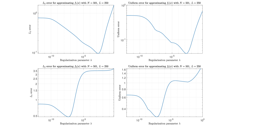
In all our experiments, we assume that the set of points is the set of equidistant points on $(-\pi,\pi],$ and when we choose parameters by three algorithms in section 5, we keep the relation of points number $N$ and the degree of approximation trigonometric polynomial (3.7) $L$ satisfy $2L+1=N.$ On the one hand, we wish fix degree $L$ so that we could compare these algorithms conveniently, on the other hand, the Morozov’s discrepancy principle is regular under the relation $2L+1=N$ from Corollary 5.1. The range of regularization parameters given by

$\displaystyle\mathcal{S}:=\left\{\lambda=2^{i},\;i=-40,-39.9,-39.8,-39.7,\ldots,1\right\},$

and the corresponding parameters in (5.22) are $\zeta_{0}=2^{-40},\;q=2^{0.1},\;T=390.$

For each of these values of $\lambda,$ we compute the the approximation $L_{2}$ error and uniform error via $p_{\lambda,L,N}^{\beta}$ (3.7) for $f_{1}(x),\;f_{2}(x),$ and we plot these error curves in Figure 1. We can see that the proper parameter choice can improve the approximation efficiency apparently.

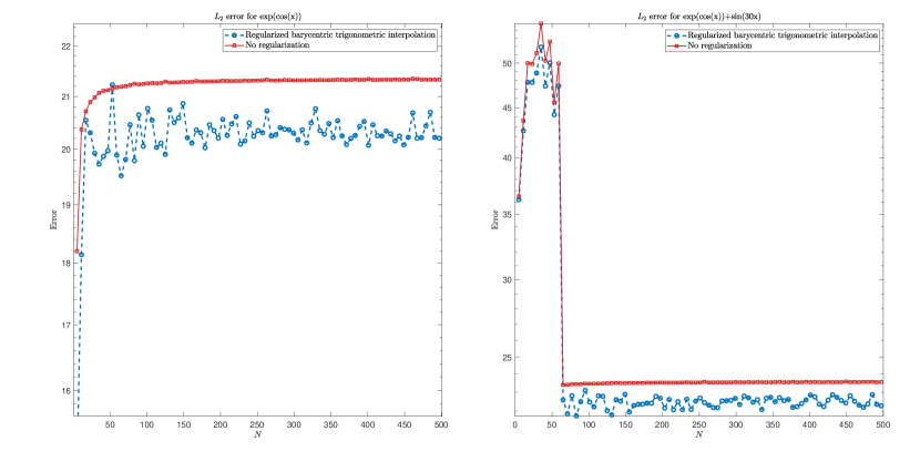
In our second experiment, we test the approximation efficiency of $f_{1}(x)$ and $f_{2}(x)$ by classical trigonometric interpolation and regularized barycentric trigonometric interpolation. We fixed noise level $\epsilon=10$ dB, and determine parameter $\lambda$ by the Morozov’s discrepancy principal. The constant $\tau$ in (3.11) is settled by $0.1d+1,$ where $d$ is noise level, i.e., how much dB noise. Figure 2 shows regularized barycentric trigonometric interpolation could indeed reduce noise which has more robustness than classical trigonometric interpolation.

To be able to apply the Morozov’s discrepancy principal, we need to verify the assumption (5.14) $\|\mathcal{L}_{L}f^{\epsilon}-f^{\epsilon}\|_{2,t_{N}}<\|\epsilon\|_{2,t_{N}}<\|f^{\epsilon}-\sigma\|_{2,t_{N}}.$ Keeping the same setting with above, we just compute the value $J(\lambda)$ of $f_{1}(x),\;f_{2}(x)$ with the range $J(\mathcal{S})$ and noise level $\|\epsilon\|_{2,t_{N}}.$ Figure 2 shows that $\|\epsilon\|_{2,t_{N}}$ is exactly in the range $J(\mathcal{S}),$ which means that the assumption is satisfied naturally.
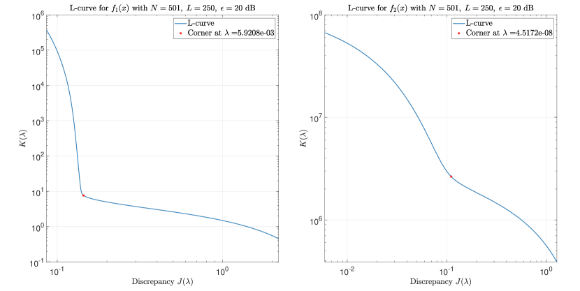
Then we give the whole log-log plot of $\left(J(\mathcal{S}),K(\mathcal{S})\right)$ for $f_{1}(x),\;f_{2}(x)$ with 20 dB noise. Figure 3 shows that these two plots are exactly L shaped, and the L corner of $f_{1}(x)$ is more apparent than $f_{2}(x).$

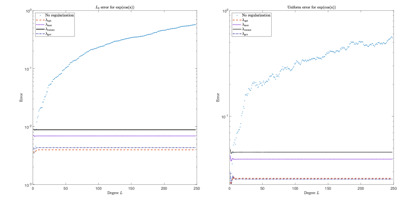
In order to compare the efficiency of three parameter choice strategies, we test $f_{1}(x)$ with 20 dB noise at first, setting the parameter $\lambda$ from $\mathcal{S}$ such that the $L_{2}$ error of $p_{\lambda,L,N}^{\beta}$ minimal be the best choice $\lambda_{{\rm opt}}.$ Fix $N=501,$ computing parameter $\lambda_{{\rm mor}},\;\lambda_{{\rm corner}},\;\lambda_{{\rm gcv}}.$ Then increasing degree $L$ from $3$ to $250$ with step $1.$ Figure 4 shows the approximation trigonometric polynomial $p_{\lambda,L,N}^{\beta}$ obtained by three parameter choice strategies can reduce $L_{2}$ error and uniform error significantly, and GCV is more advance than other two methods, since it’s error curve could nearly overlap with $\lambda_{{\rm opt}}$ for $f_{1}(x)$.

We also compare regularized trigonometric polynomial $p_{\lambda,L,N}^{\beta}$ to Lasso trigonometric interpolation $\mathcal{T}_{L}^{\lambda}f$ [1], which is a sparse trigonometric approximation. Figure 5 shows both trigonometric approximations can recover periodic function well, but there exists Gibbs phenomenon for Lasso trigonometric interpolation. In [1], the authors combine Lasso trigonometric interpolation and Lanczos $\sigma$ factor to reduce oscillation. It seems that the $\ell_{2}^{2}$ penalty could also overcome some oscillations.

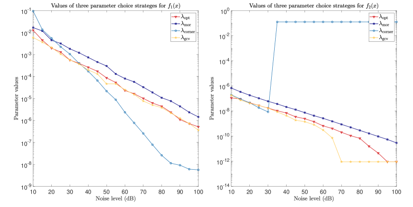
To test these parameter choice strategies for different noise level. We let the same setting with above experiments, then adding a decreasing sequence of noise from 10 dB to 100 dB with step 5 dB to $f_{1}(x)$ and $f_{2}(x).$ Semilogying corresponding parameter values $\lambda_{{\rm opt}},\;\lambda_{{\rm mor}},\;\lambda_{{\rm corner}},\;\lambda_{{\rm gcv}}$ respectively. The first column of Figure 6 shows GCV is best parameter choice strategy as it’s parameter curve convergent with nearly same rate of optimal parameter curve. The Morozov’s discrepancy principal is relative reliable as it’s parameter curve close to optimal parameter. The L-curve method is reliable just for limited range of noise. However, for seriously noise contamination, L-curve method performed better than Morozov’s discrepancy principal. The second column shows L-curve and GCV are not regular. Conversely, Morozov’s discrepancy principal is regular for both functions, which verifies the conclusion of Corollary 5.1. In practice, we should avoid using L-curve for case of low noise level, instead, the Morozov’s discrepancy principal is stable under that situation. In one word, we need to choose these three strategies according to roughly noise level.

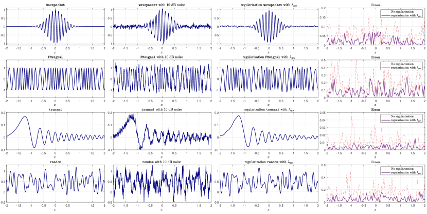
At last, we test the recovery efficiency of continuous periodic function by approximation trigonometric polynomial $p_{\lambda,L,N}^{\beta}.$ To achieve this target, we choose more general examples, which are from CHEBFUN 5.7.0 [44]. In this tool, the command cheb.gallerytrig(’name’) can provide several classical periodic functions and we just select following four gallery functions as our testing examples:

$\displaystyle\texttt{'wavepacket'}:\;\;\;\;\;{\rm Cosine\;modulated\;by\;Gaussian},$
$\displaystyle\texttt{'FMsignal'}:\;\;\;\;\;\quad{\rm Signal\;with\;modulated\;frequency},$
$\displaystyle\texttt{'tsunami'}:\;\;\;\;\;\;\;\quad{\rm Solution\;to\;periodic\;ODE},$
$\displaystyle\texttt{'random'}:\;\;\;\;\;\qquad{\rm Trigonometric\;interpolant\;through\;random\;date},$

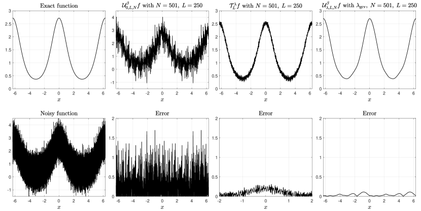
for more details about gallery functions, we see [47]. We disturb above four functions with 10 dB Gauss white noise, and we use GCV to determine regularization parameter since it could let us be free from considering the assumption (5.14) and meanwhile keeping most ideal approximation to optimal parameter. Figure 7 shows the approximation scheme (3.7) with parameter $\lambda_{{\rm corner}}$ can recovery general continuous periodic function well.

Refer to caption
Figure 1: $L_{2}$ errors (left) and uniform errors (right) as a function of $\lambda$ for the trigonometric polynomial (3.7) approximation to $f_{1}$ and $f_{2}$ with $N=501,\;L=250,\;s=2$ and 20 dB noise.
Refer to caption
Figure 2: $L_{2}$ errors for the trigonometric interpolation and regularized trigonometric interpolation (3.11) approximation to $f_{1}$ and $f_{2}$ with different interpolation points number $N$ and 10 dB noise.
Refer to caption
Figure 3: L-curve method: log-log plot of $K(\lambda)$ against $J(\lambda)$ for $f_{1},\;f_{2}$ with $N=501,\;L=250,\;s=2$ and 20 dB noise.
Refer to caption
Figure 4: The figure presents $L_{2}$ errors and uniform errors for $f_{1}(x)$ with 20 dB Gauss white noise. The errors are plotted in no regularization and regularization with three parameter choice strategies. Note that the error curves of GCV and error curves $\lambda_{{\rm opt}}$ nearly overlap each other.
Refer to caption
Figure 5: Approximation results of $f_{1}(x)$ with 10 dB Gauss white noise via trigonometric polynomial without regularization $\mathcal{U}_{0,L,N}^{\beta}f,$ Lasso trigonometric interpolation $\mathcal{T}_{L}^{\lambda}f$, regularized trigonometric polynomial $\mathcal{U}_{\lambda,L,N}^{\beta}f$ with parameter $\lambda_{{\rm gcv}}.$
Refer to caption
Figure 6: Convergence rates of $\lambda_{{\rm opt}},\;\lambda_{{\rm mor}},\;\lambda_{{\rm corner}}$ for $f_{1}(x)$ and $f_{2}(x)$ as noise $\epsilon$ tent to zero.
Refer to caption
Figure 7: Recovery efficiency of four gallery periodic functions come from CHEBFUN with 10 dB Gaussian white noise by approximation scheme $p_{\lambda,L,N}^{\beta}$ (3.7) with parameter $\lambda_{\rm gcv}.$

7 Concluding remarks

In this paper, a $\ell^{2}_{2}$-regularized least squares approximation is studied for recovering periodic functions with contaminated data. The explicit solution is presented with the factor $1/(1+\lambda\beta_{\ell,k}),$ which reveals the importance of how to obtain a regularization parameter. Under the interpolation condition, a regularized barycentric trigonometric interpolation scheme is formulated. It provides a new tool to recover periodic function with noisy values by means of a trigonometric interpolation. The nodes used in approximation are $N$th roots of unity [45] which can formulate the trapezoidal rule. In future study, one can relax the trapezoidal rule by Marcinkiewicz–Zygmund measure [26, 27, 28, 29, 30, 31]. This relaxation makes more nodes could be candidates to construct quadrature rules [5, 29].

From numerical examples, a proper choice of the regularization parameter $\lambda$ corresponding to noise type is able to improve the approximation quality tremendously. For different information of noises, three well-known strategies are investigated. The main advantage of the Morozov’s discrepancy principal is that it could deal with lower noise case as it’s special regular property, but this method needs to satisfy special assumption and relies on the concrete noise level of contaminated data priori. Conversely, L-curve and GCV does not require any noise level information, these methods are just designed by function data $f^{\epsilon}(x_{j}),$ but it might fail to low noise level case, which is not stable than the Morozov’s discrepancy principal. Hence, we need to select parameter choice strategy under practical noise information.

References

  • [1] An, C., and Cai, M. Lasso trigonometric polynomial approximation for periodic function recovery in equidistant points. Applied Numerical Mathematics 194 (2023), 115–130.
  • [2] An, C., Chen, X., Sloan, I. H., and Womersley, R. S. Regularized least squares approximations on the sphere using spherical designs. SIAM Journal on Numerical Analysis 50, 3 (2012), 1513–1534.
  • [3] An, C., and Wu, H.-N. Tikhonov regularization for polynomial approximation problems in Gauss quadrature points. Inverse Problems 37, 1 (2020), 015008.
  • [4] An, C., and Wu, H.-N. Lasso hyperinterpolation over general regions. SIAM Journal on Scientific Computing 43, 6 (2021), A3967–A3991.
  • [5] An, C., and Wu, H.-N. On the quadrature exactness in hyperinterpolation. BIT Numerical Mathematics 62, 4 (Dec 2022), 1899–1919.
  • [6] Aronszajn, N. Theory of reproducing kernels. Transactions of the American Mathematical Society 68, 3 (1950), 337–404.
  • [7] Austin, A. P., and Xu, K. On the numerical stability of the second barycentric formula for trigonometric interpolation in shifted equispaced points. IMA Journal of Numerical Analysis 37, 3 (08 2016), 1355–1374.
  • [8] Bakushinskii, A. Remarks on choosing a regularization parameter using the quasi-optimality and ratio criterion. USSR Computational Mathematics and Mathematical Physics 24, 4 (1984), 181–182.
  • [9] Berrut, J. P. Baryzentrische formeln zur trigonometrischen interpolation (i). Zeitschrift für angewandte Mathematik und Physik ZAMP 35, 1 (1984), 91–105.
  • [10] Berrut, J.-P., and Trefethen, L. N. Barycentric Lagrange interpolation. SIAM Review 46, 3 (2004), 501–517.
  • [11] Cultrera, A., and Callegaro, L. A simple algorithm to find the L-curve corner in the regularisation of ill-posed inverse problems. IOP SciNotes 1, 2 (aug 2020), 025004.
  • [12] DeVore, R., and Lorentz, G. Constructive Approximation. Grundlehren der mathematischen Wissenschaften. Springer-Verlag, 1993.
  • [13] Golub, G. H., Heath, M., and Wahba, G. Generalized cross-validation as a method for choosing a good ridge parameter. Technometrics 21, 2 (1979), 215–223.
  • [14] Golub, G. H., and von Matt, U. Generalized cross-validation for large-scale problems. Journal of Computational and Graphical Statistics 6, 1 (1997), 1–34.
  • [15] Hanke, M. Limitations of the L-curve method in ill-posed problems. BIT Numerical Mathematics 36, 2 (1996), 287–301.
  • [16] Hansen, P. C. Analysis of discrete ill-posed problems by means of the L-curve. SIAM Review 34, 4 (1992), 561–580.
  • [17] Hansen, P. C. The L-curve and its use in the numerical treatment of inverse problems. Computational Inverse Problems in Electrocardiology 4 (01 2001), 119–142.
  • [18] Hansen, P. C. Regularization tools version 4.0 for matlab 7.3. Numerical Algorithms 46, 2 (2007), 189–194.
  • [19] Hansen, P. C., and O’ Leary, D. P. The use of the L-curve in the regularization of discrete ill-posed problems. SIAM Journal on Scientific Computing 14, 6 (1993), 1487–1503.
  • [20] Henrici, P. Barycentric formulas for interpolating trigonometric polynomials and their conjugates. Numerische Mathematik 33, 2 (1979), 225–234.
  • [21] Hesse, K., and Le Gia, Q. T. ${L}_{2}$ error estimates for polynomial discrete penalized least-squares approximation on the sphere from noisy data. Journal of Computational and Applied Mathematics 408 (2022), 114118.
  • [22] Hesse, K., and Sloan, I. H. Hyperinterpolation on the sphere. In: Frontiers in Interpolation and Approximation(Dedicated to the Memory of Ambikeshwar Sharma) (eds.: N. K. Govil, H. N. Mhaskar, Ram N. Mohapatra, Zuhair Nashed and J. Szabados). Champman $\&$ Hall/CRC (2006), 213–248.
  • [23] Jackson, D. Über die Genauigkeit der Annäherung stetiger Funktionen durch ganze rationale Funktionen gegebenen Grades und trigonometrische summen gegebener Ordnung. Göttingen: Dieterich, 1911.
  • [24] Kress, R. Numerical Analysis. Graduate Texts in Mathematics vol 181. Springer, New York, 1998.
  • [25] Lu, S., and Pereverzev, S. Regularization Theory for Ill-posed Problems: Selected Topics. Inverse and ill-posed problems series. Walter de Gruyter GmbH & Company KG, 2013.
  • [26] Mhaskar, H. N. Polynomial operators and local smoothness classes on the unit interval. Journal of Approximation Theory 131, 2 (2004), 243–267.
  • [27] Mhaskar, H. N. Polynomial operators and local smoothness classes on the unit interval, ii. Jaen Journal on Approximation Theorem 1 (2005), 1–25.
  • [28] Mhaskar, H. N. A direct approach for function approximation on data defined manifolds. Neural Networks 132 (2020), 253–268.
  • [29] Mhaskar, H. N., Narcowich, F. J., and Ward, J. D. Spherical Marcinkiewicz–Zygmund inequalities and positive quadrature. Mathematics of Computation 70, 235 (2001), 1113–1130.
  • [30] Mhaskar, H. N., Naumova, V., and Pereverzyev, S. V. Filtered Legendre expansion method for numerical differentiation at the boundary point with application to blood glucose predictions. Applied Mathematics and Computation 224 (2013), 835–847.
  • [31] Mhaskar, H. N., Pereverzyev, S. V., and van der Walt, M. D. A deep learning approach to diabetic blood glucose prediction. Frontiers in Applied Mathematics and Statistics 3 (2017), 14.
  • [32] Morozov, V. A. On the solution of functional equations by the method of regularization. Doklady Mathematics 7 (1966), 414–417.
  • [33] Nursultanov, E. D. Nikol’skii’s inequality for different metrics and properties of the sequence of norms of the Fourier sums of a function in the Lorentz space. Proceedings of the Steklov Institute of Mathematics 255, 1 (2006), 185–202.
  • [34] Pereverzyev, S. An introduction to artificial intelligence based on reproducing kernel Hilbert spaces. Springer Nature, 2022.
  • [35] Pereverzyev, S. V., Sloan, I. H., and Tkachenko, P. Parameter choice strategies for least-squares approximation of noisy smooth functions on the sphere. SIAM Journal on Numerical Analysis 53, 2 (2015), 820–835.
  • [36] Rodriguez, G., and Theis, D. An algorithm for estimating the optimal regularization parameter by the L-curve. Rendiconti di Matematica, Serie VII 25 (01 2005), 69–84.
  • [37] Salzer, H. E. Coefficients for facilitating trigonometric interpolation. Journal of Mathematics and Physics 27 (1948), 274–278.
  • [38] Sloan, I. Polynomial interpolation and hyperinterpolation over general regions. Journal of Approximation Theory 83, 2 (1995), 238–254.
  • [39] Sloan, I. H. Polynomial approximation on spheres - generalizing de la Vallée-Poussin. Computational Methods in Applied Mathematics 11, 4 (2011), 540–552.
  • [40] Stein, E., and Shakarchi, R. Fourier Analysis: An Introduction. Princeton Lectures in Analysis. Princeton University Press, 2003.
  • [41] Stilson, T. S., and Smith, J. O. Alias-free digital synthesis of classic analog waveforms. In International Conference on Mathematics and Computing (1996).
  • [42] Tikhonov, A., and Glasko, V. Use of the regularization method in non-linear problems. USSR Computational Mathematics and Mathematical Physics 5, 3 (1965), 93–107.
  • [43] Tikhonov, A. N., and Arsenin, V. J. Solutions of ill-posed problems. Winston & Sons, Washington, D.C., 1977.
  • [44] Trefethen, L. N., et al. Chebfun Version 5.7.0. Chebfun Development Team, 2017.
  • [45] Trefethen, L. N., and Weideman, J. A. C. The exponentially convergent trapezoidal rule. SIAM Review 56, 3 (2014), 385–458.
  • [46] Vogel, and R, C. Non-convergence of the L-curve regularization parameter selection method. Inverse Problems 12, 4 (1996), 535–547.
  • [47] Wright, G. B., Javed, M., Montanelli, H., and Trefethen, L. N. Extension of chebfun to periodic functions. SIAM Journal on Scientific Computing 37, 5 (2015), C554–C573.
  • [48] Zygmund, A. Trigonometric Series. Cambridge Mathematical Library. Cambridge University Press, 2002.