subsecref\newrefsubsecname = \RSsectxt \RS@ifundefinedthmref\newrefthmname = theorem \RS@ifundefinedlemref\newreflemname = lemma
Sinc method in spectrum completion and inverse Sturm-Liouville problems
Abstract
Cardinal series representations for solutions of the Sturm-Liouville equation , with a complex valued potential are obtained, by using the corresponding transmutation operator. Consequently, partial sums of the series approximate the solutions uniformly with respect to in any strip of the complex plane. This property of the obtained series representations leads to their applications in a variety of spectral problems. In particular, we show their applicability to the spectrum completion problem, consisting in computing large sets of the eigenvalues from a reduced finite set of known eigenvalues, without any information on the potential as well as on the constants from boundary conditions. Among other applications this leads to an efficient numerical method for computing a Weyl function from two finite sets of the eigenvalues. This possibility is explored in the present work and illustrated by numerical tests.
Finally, based on the cardinal series representations obtained, we develop a method for the numerical solution of the inverse two-spectra Sturm-Liouville problem and show its numerical efficiency.
Vladislav V. Kravchenko1, L. Estefania Murcia-Lozano1
1Departamento de Matemáticas, Cinvestav, Unidad Querétaro
Libramiento Norponiente #2000, Fracc. Real de Juriquilla, Querétaro, Qro. C.P. 76230 México
vkravchenko@math.cinvestav.edu.mx, emurcia@math.cinvestav.mx
Keywords: Non-selfadjoint Schrödinger operator; cardinal series representations; spectrum completion; two-spectra inverse Sturm-Liouville problems; Weyl function
1 Introduction
Let be complex valued, . Consider the Sturm-Liouville equation
| (1) |
where is a spectral parameter.
Let and be the solutions of (1) satisfying the initial conditions
for all . For any fixed, and as functions of , the functions and are entire and, moreover, belong to the Paley-Wiener class . This is because of the existence of the -functions and , such that
and
for all . These Volterra integral operators of the second kind are known as transmutation or transformation operators and play a key role in spectral theory and theory of inverse problems. For their theory we refer to [58], [59], [60] and [77].
Several different series representations for the solutions and are known. The spectral parameter power series (SPPS) representations (see [43], [44], [45], [46], [47], [52] and references therein) give the solutions and in the form of power series in terms of . The coefficients of the series are calculated following a simple recurrent integration procedure and in fact, they are nothing but the images of the Taylor series coefficients of the functions and under the action of the respective transmutation operators. The SPPS converge uniformly in any compact set of the complex -plane and find numerous applications when solving direct spectral problems (we refer to the review [47] and references in [52, p. 11]).
In [50], by expanding the kernels and into series of Legendre polynomials, the Neumann series of Bessel functions (NSBF) representations for and were obtained (equalities (16) and (17) below). They proved to be extremely useful for solving both the direct and the inverse spectral problems for (1) (see [50], [52], [55], [56]) due to a couple of very convenient properties: they converge uniformly with respect to (in fact, with respect to belonging to a strip ), and the first coefficient of the series is sufficient to reconstruct the potential . In [56], for continuously differentiable potentials other NSBF representations for the solutions and were derived, which not only converge uniformly with respect to but also admit estimates for the remainders of the series which guarantee even the improvement of the convergence for large values of (). They were used for solving a variety of inverse coefficient problems for (1).
The belonging of the functions and to the Paley-Wiener class , due to the Whittaker-Shannon-Kotelnikov sampling theorem, naturally leads to their representations in the form of cardinal series (involving the function, see e.g., [34], [61], [76] and [78]). They were used for solving direct Sturm-Liouville problems in a number of papers, e.g., [8, Chapter 10], [12], [13], [14], [22], [26], [31], [74], and associated with a general Sinc method for ordinary and partial differential equations, e.g., [3], [4], [61], [67], [72], [73] and references therein, [75].
In the present paper we develop the Sinc method by obtaining new cardinal series for the solutions and and applying them to the spectrum completion, to the computation of Weyl’s function from two spectra as well as to the solution of the two-spectra inverse Sturm-Liouville problem.
The spectrum completion refers to a technique which allows one to compute a large set of the eigenvalues of a Sturm-Liouville problem from several given eigenvalues, without knowing the potential . This possibility was explored in [55] for real-valued potentials, and with the aid of the NSBF representations. It was shown that this technique gives more accurate results than, e.g., implementing well known asymptotic formulas for the eigenvalues. In the present work we show that the cardinal series representations for the solutions are also applicable to this problem, including the spectrum completion for complex valued potentials. Comparison with the NSBF series shows that the cardinal series are even preferable for dealing with noisy data. The approach is based on converting the knowledge of several eigenvalues into the series representation coefficients of the characteristic function. Due to the uniform convergence of the series in strips (), this gives us the possibility to compute large sets of zeros of the characteristic function, thus completing the spectrum. The same idea is used in the present work for computing the Weyl function from the corresponding two spectra. The Weyl function can be regarded as a quotient of two characteristic functions of Sturm-Liouville problems, and for its calculation there are known analytical formulas (see, e.g., [29], [33, Lemma 4.1]) which unfortunately are not of a practical applicability. In the present work we use the known eigenvalues from two spectra for computing the coefficients of the characteristic functions, that leads to a simple and efficient method for computing the corresponding Weyl function.
Finally, we develop a method for solving the classical two-spectra inverse Sturm-Liouville problem, which consists in the recovery of a potential and boundary conditions from the spectra of two different Sturm-Liouville problems for (1).
This problem has been extensively studied (see, e.g., [11], [21], [52], [69]), even in the case of a complex valued potential , (see, [10], [18], [29], [36], [56], [62]). It encounters practical applications across various fields (see, e.g., [6], [32]).
In a number of publications numerical methods for the two-spectra inverse problems have been developed, see, e.g., [21], [30], [42], [53], [54], [55], [64], [68] and [69], however, for real-valued potentials. It is worth mentioning that [53] was the first work where a numerical method developed allowed recovering the boundary conditions. Here we present a method for the numerical solution of the two-spectra inverse problems for complex potentials, developing a recent result from [56], where an approach to solving inverse coefficient problems for complex potentials was proposed. Moreover, to our best knowledge the present work is the first one, in which the application of the Sinc method to the inverse spectral problems is developed.
The paper is structured as follows. In Section 2 we introduce necessary notations, definitions and properties concerning the transmutation operators. In Section 3 we introduce the NSBF representations together with their basic properties. In Section 4, Fourier expansions of the transmutation kernels and the Whittaker–Shannon–Kotelnikov sampling theorem are used to obtain one of the main results of this work, the cardinal series representations, Theorem 8 and Theorem 18. Additionally, analogous results are obtained for the derivatives of solutions of (1). Section 5 presents an approach for solving the spectrum completion problem together with numerical results and discussion. In Section 6 an approximation of the Weyl function from two spectra of (1) using Sinc methods is discussed. Section 7 presents an approach for solving the two-spectra inverse Sturm-Liouville problem together with numerical illustrations. Finally, Section 8 presents some concluding remarks.
2 Preliminaries
By , , and we denote the solutions of (1) satisfying the initial conditions
respectively, where and are some complex constants.
Denote
We will use the notation and for the partial derivatives with respect to the first or second argument, respectively ( and for the second derivatives).
We recall the integral representations for and arising in the theory of transmutation operators (see, e.g., [52], [60], [71], [77]).
Theorem 1.
Let . There exist functions and defined in the domain such that
| (2) | ||||
| (3) |
for all . The functions and possess the same regularity as , see [29, p. 22]. In particular, (), see the proof of Proposition 19 in [20].
The derivatives of and with respect to admit the integral representations
| (4) | ||||
| (5) |
for , where , .
Assume, . The transmutation kernels and defined on the domain are twice differentiable with respect to each of the arguments and satisfy the equalities [48]
| (6) | ||||
| (7) |
| (8) |
| (9) |
and
where .
Theorem 2.
Let . The solutions and admit the integral representations
| (10) | ||||
| (11) | ||||
3 Neumann series of Bessel functions representations
In [50] the following Neumann series of Bessel functions (NSBF) representations for solutions and of (1) were obtained:
| (16) | ||||
| (17) |
where stands for the spherical Bessel function of order (see, e.g., [1, p. 437]). The coefficients and can be calculated following a simple recurrent integration procedure (see [50] or [52, Sect. 9.4]). For every the series converge pointwise, and for every the convergence is uniform on any compact set of the complex plane of the variable .
Since in this work we deal with several series representations for solutions of (1), we need to introduce notations for the corresponding partial sums. The partial sums of (16) and (17) are denoted by
| (18) | ||||
| (19) |
For any belonging to the strip , the inequalities hold [50]
Here and everywhere below the same symbol stands for a positive function tending to zero when , which is independent of . Note that and .
Thus, the remainders of the partial sums admit estimates, which are independent of the real part of . This is extremely useful when using the partial sums as approximate solutions for solving direct or inverse problems on large ranges of the spectral parameter.
For smooth potentials () another NSBF representation for and was obtained in [56] with the aid of results from [51].
Hereinafter, denote
Theorem 3.
Let . The solutions and of equation (1) admit the following representations
| (20) |
and
| (21) |
For every the series in (20) and (21) converge pointwise, and for every the convergence is uniform on any compact set of the complex plane of the variable . Moreover, for any belonging to the strip , the estimates hold
| (22) |
where
| (23) |
and is a positive function tending to zero when .
We notice that the estimates (22) guarantee an ever-improving accuracy of the approximation by the partial sums for larger values of .
4 Cardinal series representations for solutions
To obtain the cardinal series representations used in the present work, we start with the Fourier series expansions of the transmutation kernels and .
Proposition 5.
The transmutation kernel admits the series representation
| (25) |
where for every the series converges absolutely and uniformly with respect to .
Proof.
For any fixed, formula (25) is nothing but a Fourier expansion in terms of the orthonormal basis of , see [28, p. 80, Ex. 6]. In fact, this expansion can be seen as a classical Fourier sine series. For this, extend onto by making it symmetric with respect to the line , that is, define the extension as for . Then consider the odd extension of onto . Thus, we obtain a function . Since is square integrable, its Fourier series converges absolutely and uniformly, see [7, Chap.1. §26]. ∎
Proposition 6.
The transmutation kernel admits the series representation
| (26) |
where for every the series converges absolutely and uniformly with respect to .
Proof.
For any , with being square integrable. Let us consider the even extension of onto and its cosine Fourier expansion in the orthonormal basis . Since is square integrable, its Fourier series converges absolutely and uniformly, see [7, Chap.1. §26]. ∎
Remark 7.
It is worth to mentioning the compatibility of the Fourier series representation (25) with the condition (6) at the point , i.e., direct substitution of into (25) gives us . Moreover, the condition at from (6) implies
Analogously,
4.1 Cardinal series representation for solutions of (1) with
Recall the Paley-Wiener class and its orthonormal basis . The function stands for the normalized sinc function defined as
The Whittaker-Shannon-Kotel’nikov (W.S.K) sampling theorem asserts that a function belonging to the Paley-Wiener class admits the series representation
| (27) |
The series (27) is known as the cardinal series of and converges uniformly on compact subsets of . For on the real line, the convergence of this series holds in the norm of , absolutely and uniformly, see [34, p. 59].
Theorem 8.
Let . The solutions and of equation (1) admit the following series representations
| (28) |
where
| (29) |
and
| (30) |
where
| (31) |
The series in (28) and (30) converge uniformly on any compact subset of the complex plane of the variable . For on the real line, the convergence of (28) and (30) holds in the norm of , absolutely and uniformly.
Proof.
According to (3), for any fixed value of , the function
| (32) |
belongs to the Paley-Wiener class . By the W.S.K theorem, it is represented by the cardinal series
| (33) |
The coefficients , are obtained as the values of the function at the sample points i.e.,
Finally, we obtain (30) by using the identity
| (34) |
We have
| (35) |
Thus,
| (36) |
Considering , in (36), we obtain
Thus, denoting the desired cardinal series representation for the solution is obtained.
From the convergence principle (see [34, p. 57]) and W.S.K theorem, it follows that for on the real line and on any compact subset of the complex plane, the convergence of (28) and (30) holds uniformly. Additionally, the absolute convergence follows from Hölder’s inequality, see Theorem 6.16 in [34, p. 53]. ∎
Remark 9.
Remark 10.
In [12], another cardinal series representation for the function is obtained by applying the W.S.K theorem directly to the function . It can also be derived by expanding the transmutation kernel into the Fourier series
with respect to the orthogonal basis of . However, the pointwise convergence may fail in this case. Indeed, at the point the series is , which is not generally true for , see (6).
Theorem 11.
Let . The solutions and of equation (1) admit the following series representations
| (37) | ||||
where
and
| (38) | ||||
where
| (39) |
The series in (37) and (38) converge uniformly on any compact subset of the complex plane of the variable . For on the real line, the convergence holds in the norm of , absolutely and uniformly.
Proof.
The following relations between the coefficients of the NSBF representations and cardinal series representations hold.
4.2 Representation for derivatives of solutions
Theorem 14.
Proof.
The proof is analogous to the proof of Theorem 8. First, consider the kernel from (4), and its Fourier expansion in terms of the orthogonal basis in as follows
| (44) |
where for every the series converges in . Substitution of (44) into (4) and application of formula (35) leads to the cardinal series representation (41) where . Here we change the order of summation and integration due to Parseval’s identity [2, p. 16]. The formula (42) for the coefficients can be obtained applying the same procedure as for in Theorem 8.
Now, consider the function which belongs to with respect to the variable , because of (5). By the W.S.K theorem it admits the cardinal series representation
| (45) |
with the coefficients obtained as the values of the function at the sample points i.e.,
Theorem 15.
Let . The functions and admit the following representations
Proof.
The series representations are obtained from those of Theorem 14 by flipping the interval. ∎
Remark 16.
The obtained series representations for the solutions are not limited to potentials from . In [10], [37] and [38], definitions and construction of transmutation operators for potentials in are presented. Similar series representations for the integral transmutation kernels of the corresponding Volterra integral operators can be obtained in this case as well, that leads to similar cardinal series representations for the solutions.
4.3 Cardinal series representation for solutions when
Let . We obtain another cardinal series representation for the solutions , , and of equation (1) with the aid of the integral representations from Theorem 2. First, consider the following Fourier expansion of the kernel .
Proposition 17.
The kernel from (10) admits the series representation
| (48) |
where for every the series converges in .
Proof.
Theorem 18.
Let . The solutions and of equation (1) admit the following series representations
| (49) | ||||
Proof.
According to (11),
belongs to with respect to the variable . Application of the W.S.K theorem leads to the cardinal series expansion
By rewriting the series representation for in terms of the solution and noting that , we obtain
| (52) |
Analogous to the proof of the series representation (28), substitution of the Fourier series (48) into (10) leads to (49), where .
From the convergence principle (see [34, p. 57]) and the W.S.K theorem, it follows that for on the real line and on any compact subset of the complex plane, the convergence of (49) and (51) holds uniformly. Additionally, the absolute convergence follows from Hölder’s inequality, see Theorem 6.16 in [34, p. 53]. ∎
Remark 19.
Theorem 20.
Let . The solutions and of equation (1) admit the following series representations
| (54) | ||||
where
and
| (55) |
where
The series in (54) and (55) converge uniformly on any compact subset of the complex plane of the variable . For on the real line, the convergence of (54) and (55) holds in the norm of , absolutely and uniformly.
Proof.
Remark 21.
The cardinal series representation of at (as well as the other cardinal series representations of Section 4) is obtained by taking the corresponding limits:
4.4 Remainder estimates
This section presents remainder estimates of the cardinal series representations for solutions , and their derivatives. Similar results are obtained for remainder estimates of the cardinal series representations for solutions , and their derivatives.
and
respectively.
For any the following remainder estimates hold
| (57) |
| (58) |
for all and
| (59) |
| (60) |
for all belonging to the strip , where is a positive function tending to zero when , i.e., the series in (28) and (30) converge uniformly respect to the variable in any strip , .
The first estimate in (59) follows from the Cauchy–Bunyakovsky–Schwarz inequality,
Since
we obtain the inequality
| (62) |
The following inequalities are valid
for all and
for all belonging to a strip , where is a positive function tending to zero when . The proof of the estimate for is analogous to the proof (61). For , the proof of the estimate follows from the Cauchy–Bunyakovsky–Schwarz inequality, analogous to the proof of (62) (see Theorem 2.2 in [56]).
Remark 22.
The error analysis of cardinal series has been extensively investigated. For instance, in [8, p. 258] the results from [19, Section 3.5] were applied to describe the amplitude error of cardinal series for functions from the class , see also [5], [40], [41] and references therein. Recall the amplitude error
The values differ from the exact coefficients by local errors , such that , for , and there exists a constant , such that
| (65) |
Then for the estimate for the amplitude error is valid
Very often the coefficients of the cardinal series are not available in the exact form, so the amplitude error estimates allow us to estimate the error caused by working with noisy data.
Proposition 23.
Consider the approximation
of the cardinal series representation (30).
Let represent values differing from the exact coefficients by local errors , , which are uniformly bounded, , .
Then
for , , , where is a constant.
Proof.
Since (see [29, Lemma 1.1.2])
An analogous result can be obtained for the cardinal series representation of the solution since the proof of the amplitude estimate in [19, Section 3.5] can be reproduced in this case as well.
| (66) |
| (67) |
and
| (68) | ||||
respectively.
5 Spectrum completion
The approach to the spectrum completion problem is analogous to that in [55], where Neumann series of Bessel functions representations for solutions of (1) were used. Given a finite set of the eigenvalues of a Sturm-Liouville problem, the algorithm consists in computing several first coefficients of a series representation for a characteristic function of the problem, thus approximating the characteristic function and consequently locating its zeros for computing further eigenvalues.
Namely, let us assume that several eigenvalues of a Sturm-Liouville problem
| (69) |
are given, where is the unknown complex valued potential and and are unknown complex constants. The solution fulfills the second boundary condition of (69). Thus, the characteristic function of problem (69) is defined by the first boundary condition
| (70) |
where , see [29, p. 6].
The spectrum completion can be performed following the algorithm.
1. Approximate the characteristic function of problem (69) by using the truncated cardinal series representations (66) (corresponding to potentials ) and (68), i.e.,
where
| (71) |
2. Consider a system of linear algebraic equations, which is obtained from the equalities (),
with
Solving this system of equations, we obtain the coefficients
| (72) |
3. Consider the approximate characteristic function , for any . This is possible because the coefficients (72) found in the previous step are independent of .
4. Finally, compute the zeros of . Their squares approximate the eigenvalues of (69).
Notice that for completing the spectrum no knowledge of , and is required.
Remark 24.
If it is known that and not necessarily , the function is approximated by (67) (instead of (66)) in step 1 of the spectrum completion algorithm. In this case, the system of linear algebraic equations in step 2 is derived from the equalities:
where and . Solving this system of equations is sufficient to reconstruct and proceed to step 4 of the spectrum completion algorithm.
Remark 25.
In the case of a Sturm-Liouville problem involving a Dirichlet condition at or at the procedure is analogous. For example, suppose there is given a finite set of eigenvalues of the Dirichlet-Dirichlet Sturm-Liouville problem, i.e., equation (1) subject to the boundary conditions
The square roots of the eigenvalues coincide with zeros of the function . The linear system (analogous to that mentioned in step 2) of the spectrum completion algorithm can be constructed in four different forms by considering one of the four truncated series representations (18), (23), (56) and (63). In particular, by considering the system is constructed from the equations
| (73) |
Notice that the parameter is one of the components of the vector solution.
Similarly, by considering the system is obtained from the equations
The other two options or are analogous (NSBF representations are considered).
Finally, once the characteristic function (or , or , or ) is obtained, compute its zeros. Their squares provide approximations to the eigenvalues of the Dirichlet-Dirichlet problem.
Let us discuss the computation of the parameter . For this, recall that , the square roots of the eigenvalues, satisfy the asymptotic relation
| (74) |
where .
A frequently used technique for computing consists in minimizing the -norm of the sequence
| (75) |
constructed from (74), see, e.g., [39], [69]. In Section 5.1, thus obtained approximation of is compared with the value obtained as a part of the solution of system (73).
Theorem 26.
For any there exists such that all zeros of the function are approximated by corresponding zeros of the function with errors uniformly bounded by , and has no other zeros.
Proof.
The proof is analogous to the proof of Proposition 7.1 in [48] where the Rouché theorem is applied to the functions and . ∎
Remark 27.
We present illustrative examples performed in Matlab2021a. In the final step of the spectrum completion algorithm, when locating complex zeros of the approximate characteristic function, the algorithm of the argument principle theorem described in [49] is applied. When , and are real, to locate real zeros, the ’fnzeros’ routine in Matlab is used, applying it to a 6th order spline interpolation of the approximate characteristic function.
5.1 Dirichlet-Dirichlet spectrum completion
The Dirichlet-Dirichlet spectrum completion is performed following Remark 25. The first two examples of this section deal with the spectrum completion by using the four truncated series representations (18), (23), (56) and (63) in the case of real-valued potentials. In the last example, a complex Dirichlet-Dirichlet spectrum is considered, and the spectrum completion algorithm is performed by using the truncated cardinal series representations (56) and (63).
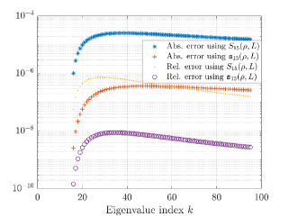
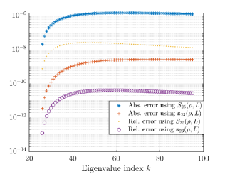
Example 1. Consider the potential , . We compute the input data (a set of the first eigenvalues) in a high precision arithmetics in Wolfram Mathematica12 in order to study different situations under the presence of a controlled noise. In Figures 5.1 and 5.2, we present the absolute errors of the Dirichlet-Dirichlet spectrum completed by using the four different approximations of , see Remark 25.
Three cases are considered, corresponding to 15, 10 and 5 eigenvalues given as input data, presented by three columns in Figure 5.1. In each case, the considered linear system of algebraic equations is square. In the first column, series representations , , and , each with 15 unknown coefficients, are used. In the second column, series representations , , and , each with 10 unknown coefficients are considered. Finally, in the third column, series representations , , and , each with 5 unknown coefficients, are considered. Furthermore, in the first row of Figure 5.1, we present the absolute errors of the computed zeros of the characteristic function when exact input data are used. The other two rows of the grid present the absolute errors dealing with randomly noisy data, as indicated at the top of each figure. In all the cases we complete the sequence of the first 300 eigenvalues.
For convenience we use the following notation. indicates the use of expression (18), refers to the use of (23), indicates the use of (56) and refers to the use of (63).
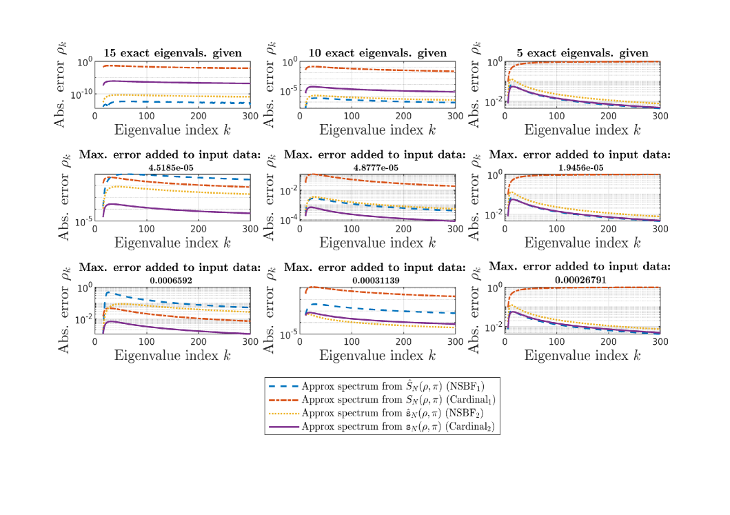
The results in the first row of Figure 5.1 indicate a better accuracy attained by both NSBF representations and by the cardinal series representation (63). When the input data are not exact, the cardinal series representation (63) turns to be a preferable technique (see the second and the third rows of figure 5.1).
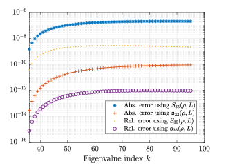
In Figure 5.2, three numerical tests are reported. Here in all tests 15 eigenvalues are given, however, we deal with the partial sums of the series representations containing less coefficients, thus solving overdetermined systems of linear algebraic equations. The results presented in the first column correspond to the partial sums , , and . For each of these partial sums 13 unknown coefficients are computed from a system. Analogously, the results of the second column correspond to the partial sums , , and , while the results of the third column correspond to , , and . In the first row, the absolute errors presented correspond to exact input data. The other two rows of the grid present the absolute errors corresponding to noisy data as indicated at the top of each figure.
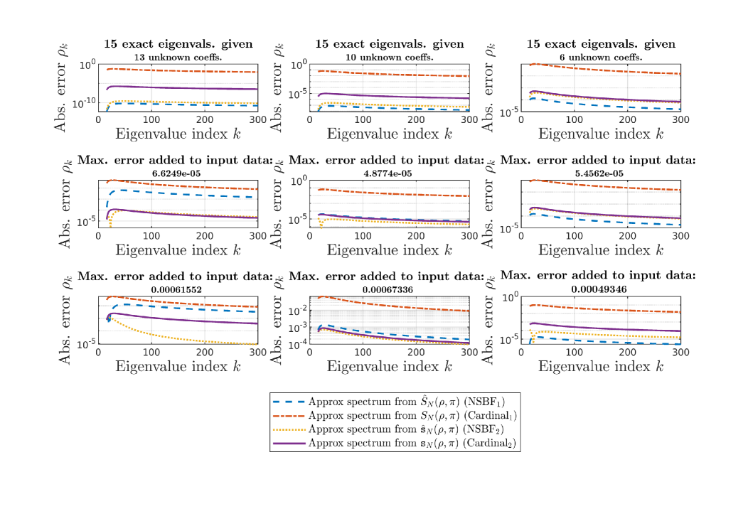
Figure 5.2 shows that both NSBF representations and the cardinal series representation (63) provide comparable accuracy when dealing with fewer coefficients and noisy data.
Given 15 exact eigenvalues, the value of was obtained by using and as shown in Table 1.
| Minimizing -norm of | NSBF series | Cardinal series | |
|---|---|---|---|
| the sequence, see (75) | |||
| Abs. error | |||
| Rel. error |
Note that the spectrum completion algorithm demonstrates a remarkable accuracy in approximating the parameter as compared to the minimization of the -norm of , see (75).
Example 2. Consider the potential , . The “exact” eigenvalues were computed by the Matslise package [57]. In Figures 5.3 and 5.4, the absolute error of the Dirichlet-Dirichlet spectrum completed by using the four different approximations of is presented.
Three cases are considered, corresponding to 15, 10 and 5 eigenvalues given as input data, presented by three columns in Figure 5.3. In each case, the considered linear system of algebraic equations is square. In the first column, series representations , , and , each with 15 unknown coefficients, are used. In the second column, series representations , , and , each with 10 unknown coefficients, are considered. Finally, in the third column, series representations , , and , each with 5 unknown coefficients, are considered. Furthermore, in the first row of Figure 5.3, we present the absolute errors of the computed zeros of the characteristic function when exact input data are used. The other two rows of the grid present the absolute errors dealing with randomly noisy data, as indicated at the top of each figure. In all the cases we complete the sequence of the first 300 eigenvalues.
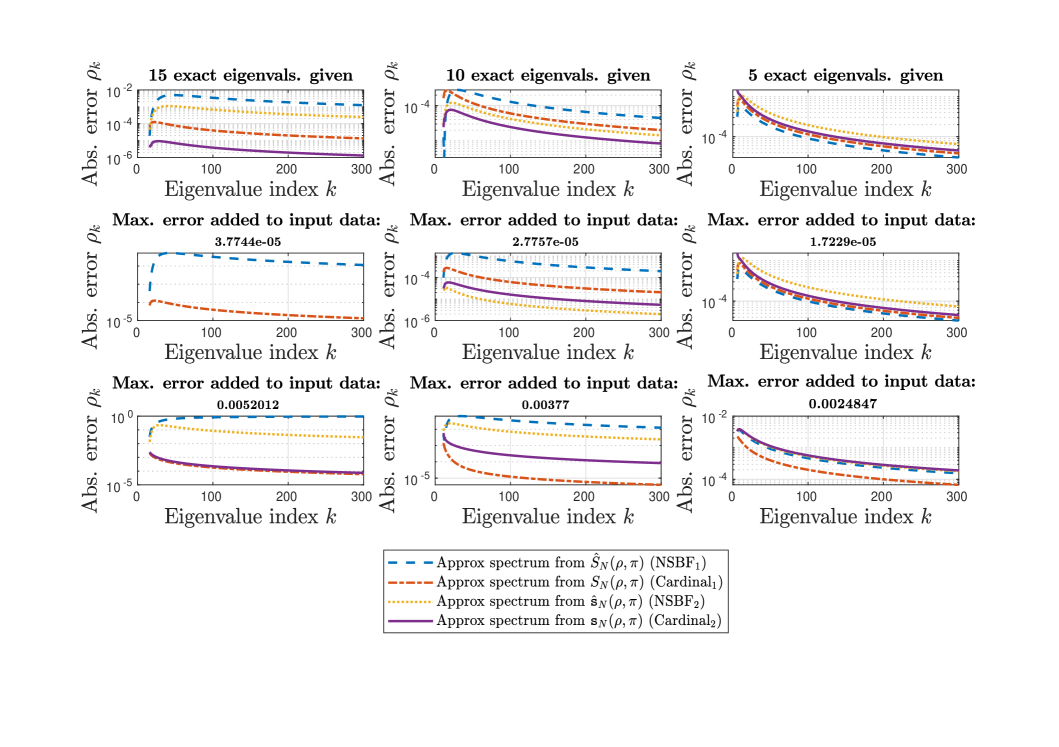
Figure 5.3 shows that both the NSBF and cardinal series representations provide comparable accuracy when dealing with fewer given eigenvalues. However, from given 15 eigenvalues (first column), better results are attained by using the cardinal series representations. Note that in the second row of the first column, the results corresponding to NSBF2 and Cardinal2 are omitted because, in both cases, in the sequence of the roots of the eigenvalues completed, one term was not found by the argument principle theorem algorithm.
In Figure 5.4, three numerical tests are reported. Here in all tests 15 eigenvalues are given, however, we deal with the partial sums of the series representations containing less coefficients, thus solving overdetermined systems of linear algebraic equations. The results presented in the first column correspond to the partial sums , , and . For each of these partial sums 13 unknown coefficients are computed from a system. Analogously, the results of the second column correspond to the partial sums , , and , while the results of the third column correspond to , , and . In the first row, the absolute errors presented correspond to exact input data. The other two rows of the grid present the absolute errors corresponding to noisy data as indicated at the top of each figure.

Figure 5.4 shows that both NSBF representations and the cardinal series representations provide comparable accuracy when dealing with fewer coefficients.
Given 15 exact eigenvalues, the value of was obtained by using and as shown in Table 2.
| Minimizing -norm of | NSBF series | Cardinal series | |
|---|---|---|---|
| the sequence | |||
| Abs. error | |||
| Rel. error |
The spectrum completion algorithm using NSBF representations attained accuracy comparable with that of minimizing the -norm of , see (75). However, in contrast to the previous example, the use of cardinal representations attained a higher accuracy in approximating .
Remark 28.
It is worth mentioning that for the numerical implementation of the spectrum completion algorithm in the case of a Sturm-Liouville problem with a real-valued potential, the input data comprise a set of several first eigenvalues. Another choice of this set, e.g., excluding some of the first eigenvalues, may affect the accuracy of the result. In examples provided below, which involve sets of complex values, the set was arranged in ascending order according to their real parts and again, another choice of the set of the input data different from the lower eigenvalues ordered in this sense, may considerably affect the accuracy of the spectrum completion results.
Example 3. Consider the potential
where . The real part of is a Razavy potential, see [65] (also [25]), while the imaginary part is a Coffey–Evans potential, see [24]. Consider the parameters and . Then exact roots of the eigenvalues of the Dirichlet-Dirichlet spectral problem were computed, i.e., , applying the argument principle algorithm to the truncated NSBF representation , see Table 3.
| 1 | 16 | ||
| 2 | 17 | ||
| 3 | 18 | ||
| 4 | 19 | ||
| 5 | 20 | ||
| 6 | 21 | ||
| 7 | 22 | ||
| 8 | 23 | ||
| 9 | 24 | ||
| 10 | 25 | ||
| 11 | 26 | ||
| 12 | 27 | ||
| 13 | 28 | ||
| 14 | 29 | ||
| 15 | 30 |
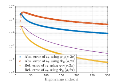
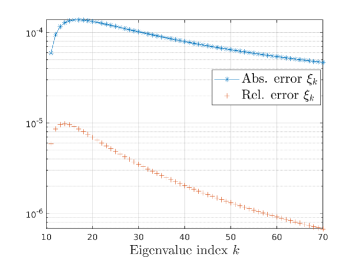
In Figure 5.5, we present the absolute and relative errors of the values computed until (a sequence of the first 95 eigenvalues were completed), from given , , and eigenvalues. The same number of the unknowns in the linear system for the coefficients of the approximate characteristic function is considered. Table 4 presents the maximum absolute and relative errors of the sequence of the completed, by using both cardinal series representations (56) and (63).
(A)
(B)
(C)
(D)
| Given 5 eigenvals. and | Given 5 eigenvals. and | Given 15 eigenvals. and | Given 15 eigenvals. and | |
|---|---|---|---|---|
| computing | computing | computing | computing | |
| Abs. error | ||||
| Rel. error |
| Given 25 eigenvals. and | Given 25 eigenvals. and | Given 35 eigenvals. and | Given 35 eigenvals. and | |
|---|---|---|---|---|
| computing | computing | computing | computing | |
| Abs. error | ||||
| Rel. error |
The results show a remarkable convergence of the method even when dealing with complex . Moreover, satisfactory results were attained with a reduced number of the eigenvalues given. Indeed, even from 5 given eigenvalues the approximate was found with an absolute error of and a relative error of .
5.2 Neumann-Dirichlet spectrum
Example 4. Consider the potential , with the parameter , see [23].
Paper [23] is devoted to the computation of energy levels and analytical wave functions for the Dirichlet-Dirichlet problem of the rigid planar rotor in an electric field model. The authors transform the Schrödinger equation into a confluent Heun differential equation and subsequently compute the eigenvalues using the Maple package. The accuracy of the algorithm relies on the numerical calculation of confluent Heun functions and their first-order derivatives by Maple. This procedure becomes complicated when a large number of eigenvalues must be computed. Thus, the spectrum completion algorithm can be useful to obtain more such data accurately.
Consider the Neumann-Dirichlet problem
| (76) |
Since the solution satisfies the first initial condition in (76), the corresponding characteristic function of the problem is approximated by (or ), see Section 4.4. Thus, given the eigenvalues (computed by Matslise), the -equations (or ) form the system of linear algebraic equations for the coefficients of the approximate characteristic function. In this example, we complete the sequence of the first 300 eigenvalues.
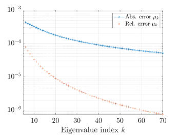
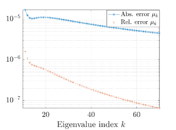
In Figures 5.7 and 5.7 the absolute errors of computed from given 5 and 15 eigenvalues are reported, respectively. In Table 5 the maximum values of the absolute and relative errors of the sequence completed are presented.
| Given 5 eigenvals. and | Given 5 eigenvals. and | Given 15 eigenvals. and | Given 15 eigenvals. and | |
|---|---|---|---|---|
| computing | computing | computing | computing | |
| Abs. error | ||||
| Rel. error |
Additionally, the parameter was computed from given 15 eigenvalues with an absolute error of .
Thus, the results of the spectrum completion are satisfactory even when the Sturm-Liouville problem is considered on a larger interval in , and a limited number of the eigenvalues is provided. The fast convergence of the method is noticeable.
5.3 Other spectra
Example 5. Consider a Sturm-Liouville problem with a Mathieu potential, see [63]
| (77) |
with assumed to be unknown. This potential with the parameter being a real constant has been studied in numerous papers (see, e.g., [15], [27, p. 44], [66] and [79]).
The solution fulfills the second boundary condition of (77). Thus, the characteristic function of the problem (77) is defined by
| (78) |
Notice also that .
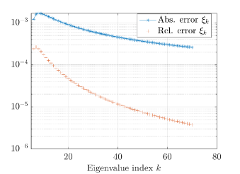
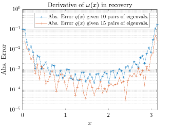
Let . The input data (a finite set of the eigenvalues of (77)) is computed with the aid of the NSBF representation (16) and its derivative (see [50]). The spectrum completion is performed by using in the algorithm, see (66). Let , given 5 eigenvalues, 65 more were computed with a maximum absolute error of , see Figure 5.9. Additionally, from 10 eigenvalues, 60 more were computed with a maximum absolute error of , see Figure 5.9. In the later case, the parameter (see (71)) was obtained with an absolute error of .
Since a good accuracy is attained even with a reduced number of given eigenvalues, the information obtained may result to be useful for solving other problems related with the same Sturm-Liouville equation, e.g., to the spectrum completion of another set of the eigenvalues corresponding the same Sturm-Liouville equation with other boundary conditions (see problem (79) below).
Now, assume there is given the set of eigenvalues of the Sturm-Liouville problem
| (79) |
with (which is assumed to be unknown). Recall the characteristic function (70).
The knowledge of the approximate solution , and the value of (found in the spectrum completion of the eigenvalues of problem (77)) is used as known variables in the linear system (step 2 in spectrum completion algorithm) obtained from equations . Solving this system we obtain the coefficients and the value of , and then for any .
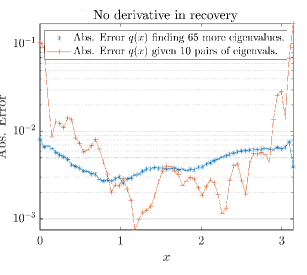
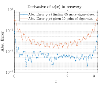
Given 5 roots of the eigenvalues (), 65 more were computed with a maximum absolute error of , see Figure 5.11. Additionally, from 10 roots of the eigenvalues () 60 more were computed with a maximum absolute error of , see Figure 5.11.
Moreover, the parameter is obtained with an absolute error of from 5 eigenvalues and with an absolute error of from 10 eigenvalues.
In this case, considerably more noise (corresponding to and ) was added to the input data forming the linear system of the spectrum completion algorithm, however, the spectrum was completed sufficiently well. Indeed, the results obtained here were applied below in Example 7, for solving a two-spectra inverse Sturm-Liouville problem for the same potential.
6 Computation of a Weyl function from two finite sets of eigenvalues
In this section we discuss the computation of the Weyl function from two spectra and corresponding to the Sturm-Liouville problems (69) and
| (80) |
respectively.
There are the well-known formulas (see [16], [17]), which in principle give us the Weyl function in terms of these sets of the eigenvalues. Namely,
| (81) |
where (see (70)) and (see (78)) are the characteristic functions of problems (69) and (80), respectively.
In Section 5 the algorithm for solving the problem of spectrum completion is presented, in which the first 3 steps consist in the computation of (procedure analogous for the computation of ) from the corresponding finite set of the eigenvalues.
Thus, in order to discuss the calculation of from (81) let us illustrate in the following example the approximation of the characteristic functions and from given corresponding sets of the eigenvalues and by using the series representation (66) in comparison with the use of the products in (81), i.e., by considering
| (82) |
and
| (83) |
For the constants and , the characteristic functions were computed with the aid of Wolfram Mathematica12. They were represented in terms of the Mathieu functions (the even solution of the Mathieu differential equation), (the odd solution of the Mathieu differential equation) and their derivatives with respect to the parameter , see [1, Ch 10.].
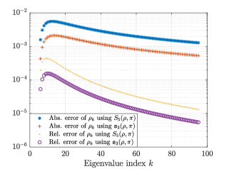
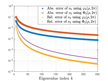
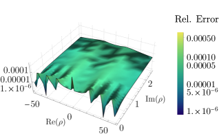
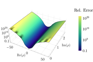
The exact eigenvalues were computed by the function to obtain the numerical roots of the corresponding characteristic functions. Figure 6.2 presents the absolute error of computed in a strip of the upper complex -plane from given 15 eigenvalues. The maximum absolute error is achieved at . In Figure 6.2 the relative error is presented. The maximum relative error achieved at is .
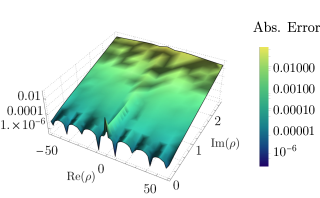
Note that the approximation of the characteristic function decreases as the absolute value of grows in the upper half-plane. In most cases these results improve if more eigenvalues are given.
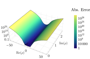
Additionally, in Figures 6.4 and 6.4, the absolute and relative errors, respectively, of computed by (82).
Analogously, similar results are obtained for computed from given 15 eigenvalues by using both the cardinal series representation and the product (83). The knowledge of , with absolute error presented in Figure 6.2, is used as input data in the linear system. A detailed explanation of this procedure was presented in Example 5.3, when dealing with the problem (79).
This simple comparison makes it obvious, that the analytical formulas (82) and (83) are not of practical usage. Instead, the series representations developed on the present work give us accurate results and indeed allow us to reconstruct the Weyl function from two finite sets of the eigenvalues.
In Figure 6.6 the approximate Weyl function computed with the aid of the cardinal series representations is presented. The corresponding absolute error of this approximation is shown in Figure 6.6.
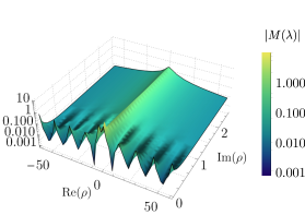
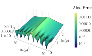
The presented results confirm that the method proposed in the first 3 steps of the spectrum completion algorithm to approximate the corresponding characteristic function has a much higher convergence than that based on the products in (81). Additionally, the Weyl function is computed accurately from 15 eigenpairs.
7 Inverse problem
In this section we discuss a method for solving the two-spectra inverse problem in which , and are complex.
Problem (two-spectra inverse problem) Given two sequences of the eigenvalues and of the Sturm-Liouville problems, respectively,
| (84) |
and
| (85) |
Find the potential and the complex constants and .
As mentioned in the previous section, a characteristic function of problem (84) is (70), and a characteristic function of problem (85) is (78).
Additionally, recall the identity satisfied by these characteristic functions
| (86) |
see [29, Formula (1.4.9), p. 29 ].
The approach developed for solving the two-spectra inverse problem develops the idea from [56], where Neumann series of Bessel functions representations for solutions of (1) were used. Our approach is based on the cardinal series representations from Section 4. The potential is recovered from the first coefficients of the representations. Moreover, two possibilities are explored. The first one involves the cardinal series from Theorem 18. Due to (53), no differentiation is required in the final step. The second one deals with the cardinal series representation from Theorem 8, and the potential is recovered from (40), which implies a double differentiation in the last step.
The algorithm to recover , and consists of the following steps.
Numerical algorithm for solving the two-spectra inverse problem for potentials from
Assume that two finite sets and of the eigenvalues of problems (84) and (85), respectively, are given.
-
1.
Consider the approximate characteristic function of problem (85) on the set , i.e.,
(87) and
Solve the finite system of linear equations derived from the equalitieswhich are obtained from (87). This gives the coefficients computed
(88) Note that, using the coefficients (88) (independent on ), the approximate characteristic function of problem (85) can be computed for any .
-
2.
Consider the approximate characteristic function on the set , i.e.,
(89) Solve the finite system of linear equations derived from the equalities
(90) which are obtained from (89). The knowledge of simplifies the system, and solving it we obtain the coefficients
(91) Note that, by using the coefficients (91) (independent on ), and obtained above, the approximate characteristic function can be computed for any .
-
3.
Substitution of (63), (64) and (66), into (86) leads to the approximate equality
(92) where different values of can be considered in each sum. Equation (92) implies
(93) where . Here, the coefficients
(94) are unknown. Then, for any construct a linear system of equations for the unknowns (94), by considering (93) evaluated at a finite set ,
(95) -
4.
For we have , so equation (92) at evaluated at a finite set has the form
where .
Solving this system we compute(96) - 5.
- 6.
The performance of the algorithm is illustrated by the following examples.
Example 7. Consider a Mathieu potential, see [63],
Let , and . For computing the spectrum of the Sturm-Liouville problems (84) and (85), the NSBF representations (16), (17) and their derivatives (see [50]) were used to approximate the corresponding characteristic functions. Additionally, to find complex zeros of the approximate characteristic function, the algorithm of the argument principle theorem was applied, see [49].
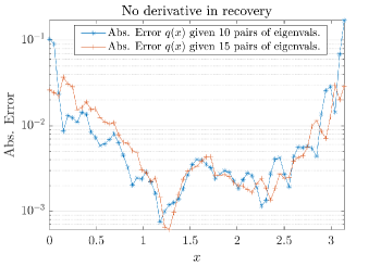
The recovery of the potential was performed from given pairs of the eigenvalues (corresponding to the Sturm-Liouville problems (84) and (85)). In step 6 of the algorithm for solving the inverse problem, both options (97) and (53) were implemented, resulting in the recovery of the potential with an absolute error of in both cases, see Figure 7.1. Using eigenpairs the potential was recovered with a maximum absolute error of see Figure 7.1. In steps 3 and 4 of the algorithm, the points and were chosen as logarithmically equally distributed on the segment , and the number in (95) was chosen as .
Furthermore, for a given set of 10 eigenpairs, the constants and were computed with the absolute errors , and , respectively. In the case of 15 eigenpairs given, the absolute errors of these constants were , and , respectively.
Now, let us consider the points in step 3 as , the square roots of the spectrum of the problem (84), i.e., is approximately , and (92) is reduced to
Hence, the number of unknowns in the system of step 3 is reduced to only those associated with and . Despite this reduction, having 10 or 15 eigenvalues is insufficient to accurately recover the coefficients (94). Therefore, in this case, the spectrum completion procedure presented in Example 5.3 results to be very useful for increasing the number of given eigenvalues as input data.
Associated to the problem (84), from 10 eigenvalues 65 more eigenvalues found by the spectrum completion algorithm were used. With this additional information the complex constants , and were found with absolute errors , and , respectively. Moreover, the potential was recovered with an absolute error with the two options (97) and (53), see Figure 7.2.
In Figure 7.3, the recovered potential (using (53)), from 10 eigenpairs and 65 more eigenvalues of problem (84) completed is presented.
This example explores the application of the spectrum completion for solving inverse problems. By using the completed eigenvalues obtained in Example 5.3, the recovery of the potential from 10 eigenpairs was considerably improved.
Example 8. Consider the potential
Ten eigenvalues of each problem (84) and (85) with the parameters and are given. The constants , and are found with the absolute errors , and , respectively, while the potential was recovered with an absolute error of (by using both options (97) and (53)), see Figure 7.4. Now, considering 18 eigenpairs, the constants , and are found with the absolute errors , and , while the potential was recovered with an absolute error , by using both options (97) and (53), see Figure 7.5. It is worth to mention that in this case, was recovered with an absolute error of . In both cases, given 10 and 18 eigenvalues, the points were chosen as logarithmically equally distributed on the segment , and the number in (95) was chosen as .
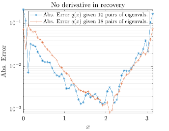
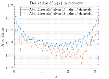
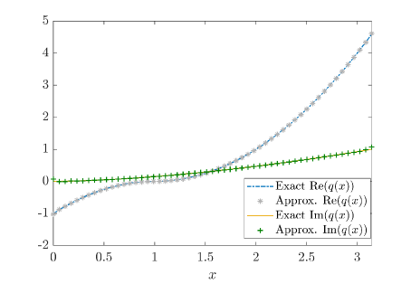
Note that the recovery of this complex valued and only once differentiable potential required only slightly more input data to attain an accuracy comparable with previous real-valued and smooth examples.
Numerical algorithm to solving the two-spectra inverse problem for potentials from
Assume that two finite sets and of the eigenvalues of problem (84) and (85), respectively, are given. The procedure is analogous to that for potentials in . The difference consists in using the cardinal series representations introduced in Section 4.1 for , and . This implies a double differentiation in the last step for the recovery of the potential.
The algorithm to recover , and consists of approximating (from the given eigenvalues) the characteristic functions and by and . Construct for any the linear system of equations by considering
| (98) |
evaluated at a finite set , i.e.,
Solving this system of equations, we obtain the coefficients
For we have , then equation (98) at evaluated at some chosen points has the form
Solving this system gives us the possibility to obtain the approximate coefficients
Finally, when the first coefficient (or ) has been computed, it is possible to recover the potential for from (40).
The performance of the algorithm is illustrated by the following example.
Example 9. Consider the potential
and parameters , in (84) and (85), i.e., the Neumann-Neumann and Dirichlet-Neumann Sturm-Liouville problems. Fifteen pairs of eigenvalues of these two problems are given. They were computed for the real part of the potential by Matslise, and a shift of them by generate the input data of the inverse problem. It is worth mentioning that these eigenvalues possess a considerable level of noise. The following simple test illustrates the situation. The first 15 eigenvalues of the Neumann-Neumann Sturm-Liouville problem with the potentials and were computed by Matslise. However, the eigenvalues obtained for and a shift by of the eigenvalues for resulted to differ by . This test reveals that the “exact” input data contain errors, possibly in the fifth digit. Nonetheless, the algorithm for solving the inverse problem allows us to recover the potential from the given noisy data. Figure 7.6 presents the recovered potential.
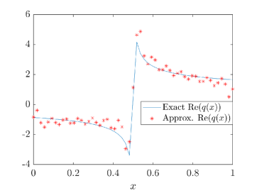
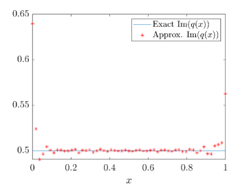
The maximum absolute error of the recovered potential is see Figure 7.7.
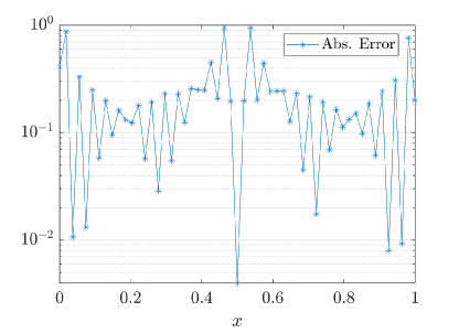
This example shows the possibility of recovering a complex valued singular potential from a limited set of noisy eigenvalues using the proposed algorithm for potentials in .
8 Conclusions
Cardinal series representations for the solutions of the Sturm-Liouville equation with a complex valued potential are obtained. They enjoy remarkable convergence properties, which make them a very convenient tool for solving a variety of spectral problems. In particular, with their aid the spectrum completion problem can be efficiently solved, allowing one to compute with a good accuracy large sets of the eigenvalues from a reduced number of the given ones and without any information on the potential and on the constants from the boundary conditions. This idea leads to an efficient computation of a Weyl function from two reduced finite sets of the eigenvalues. This application of the cardinal series representations is developed in the present paper and illustrated by numerical tests. Finally, a method for solving inverse two-spectra Sturm-Liouville problems for complex potentials is developed, based on the cardinal series representations. Its numerical efficiency is discussed and illustrated by numerical tests.
Acknowledgments Research was supported by CONAHCYT, Mexico via the project 284470. The authors thank the helpful comments of Sergii M. Torba.
Data availability The data that support the findings of this study are available upon reasonable request.
Conflict of interest This work does not have any conflict of interest.
References
- [1] M. Abramovitz and I. A. Stegun, Handbook of mathematical functions, New York: Dover, 1972.
- [2] N. I. Akhiezer, I. M. Glazman, Theory of Linear Operators in Hilbert Space, Dover, New York, 1993.
- [3] K. Al-Khaled, Sinc numerical solution for solitons and solitary waves. J. Comput. Appl. Math. 130, 283–292 (2001)
- [4] M. H. Annaby, M.M. Tharwat, On computing eigenvalues of second-order linear pencils, IMA J. Numer. Anal. 27 (2007) 366–380.
- [5] M. H. Annaby and R. M. Asharabi, On sinc-based method in computing eigenvalues of boundary-value problems, SIAM J. Num. Anal., 64, 671–690, (2008).
- [6] V. Barcilon, On the uniqueness of inverse eigenvalue problems, Geophys. J. Roy. Astron. Soc. 38 (1974) 287–298.
- [7] N. K. Bary, A Treatise on Trigonometric Series, Vol.1, Pergamon Press, New York, 1964.
- [8] G. Baumann, New Sinc Methods of Numerical Analysis: Festschrift in Honor of Frank Stenger’s 80th Birthday; Springer Nature: Cham, Switzerland, 2021.
- [9] G. Blanch, D.S. Clemm, Mathieu’s Equation for Complex Parameters: Tables of Characteristic Values. (Box 2), Aerospace Research Laboratories, Washington, DC, (1969).
- [10] N. P. Bondarenko, Inverse Sturm-Liouville problem with analytical functions in the boundary condition. Open Math. 18 (2020), 512–528.
- [11] G. Borg, Eine Umkehrunge der Sturm–Liouvillechen Eigenwertaufgabe, Acta. Math. 78 (1946) 1–96.
- [12] A. Boumenir and B. Chanane, Eigenvalues of Sturm-Liouville systems using sampling theory, Appl. Anal., 62, 323-334, (1996).
- [13] A. Boumenir, Computing Eigenvalues of periodic Sturm–Liouville problems by the Shannon–Whittaker sampling theorem. Math. Comput. 68, 1057–1066 (1999).
- [14] A. Boumenir, Sampling and eigenvalues of non-self-adjoint Sturm–Liouville problems, SIAM J. Sci. Comput. 23 (1) (2001) 219–229.
- [15] C. Brimacombe, R.M. Corless, M. Zamir, Computation and applications of Mathieu functions: a historical perspective, SIAM Rev. 63 (4) (2021) 653–720.
- [16] S.A. Buterin, On inverse spectral problem for non-selfadjoint Sturm–Liouville operator on a finite interval, J. Math. Anal. Appl. 335 (2007) 739–749.
- [17] S.A. Buterin, C.T. Shieh, V.A. Yurko, Inverse spectral problems for non-selfadjoint second-order differential operators with Dirichlet boundary conditions, Boundary Value Problems (2013): 1-24.
- [18] S. A. Buterin, M. Kuznetsova, On Borg’s method for non-selfadjoint Sturm–Liouville operators. Anal. Math. Phys. 9 (2019), 2133–2150.
- [19] P. L. Butzer, W. Splettstösser, and R. L. Stens, The sampling theorem and linear prediction in signal analysis, Jahresber. Deutsch. Math.-Verein., 90 (1988), pp. 1–70.
- [20] H. Campos, Standard transmutation operators for the one dimensional Schrödinger operator with a locally integrable potential, J. Math. Anal. Appl. 453 (2017) 1, 64–81.
- [21] K. Chadan, D. Colton, L. Päivärinta, W. Rundell, An Introduction to Inverse Scattering and Inverse Spectral Problems, SIAM, Philadelphia, 1997.
- [22] Chanane, B. Computing the spectrum of non-self-adjoint Sturm–Liouville problems with parameter-dependent boundary conditions. Journal of Computational and Applied Mathematics, 206(1), 229-237 (2007).
- [23] C.Y. Chen, F.L. Lu, G.H. Sun, X.H. Wang, Y. You, D.S. Sun & S. H. Dong. Exact solution of rigid planar rotor in external electric field. Results in Physics, 34, 105330 (2022).
- [24] M.S. Child, A.V. Chambers, Persistent accidental degeneracies for the Coffey–Evans potential, J. Phys. Chem. 92 (1988) 3122–3124.
- [25] Q. Dong, F. Serrano, G.H. Sun, J. Jing, S.H. Dong, Semiexact solutions of the Razavy potential, Adv. High Energy Phys. (2018) 9105825.
- [26] N. Eggert, M. Jarratt, J. Lund, Sinc function computation of the eigenvalues of Sturm–Liouville problems, J. Comput. Appl. Math. 69 (1987) 209–229.
- [27] S. Flügge, Practical Quantum Mechanics, Springer, Berlin, 1999, Vol. 2.
- [28] G.B. Folland, Fourier Analysis and its Applications, Brooks/Cole, New York, 1992.
- [29] G. Freiling, V. Yurko, Inverse Sturm-Liouville problems and their applications. Nova Science Publishers Inc., Huntington, NY, 2001.
- [30] Q. Gao, X. Cheng, Zh. Huang, On a boundary value method for computing Sturm–Liouville potentials from two spectra, Int. J. Comput. Math. 91 (2014), 490–513.
- [31] P. J. Gaudreau, R. M. Slevinsky, and H. Safouhi. Computing energy eigenvalues of anharmonic oscillators using the double exponential Sinc collocation method. Annals of Physics, 360:520–538, (2015).
- [32] G. M. L. Gladwell, Inverse problems in vibration. 2nd ed. Kluver Academic, New York, 2005.
- [33] B, Hatinoğlu, Mixed data in inverse spectral problems for the Schrödinger operators. Journal of Spectral Theory, 11(1), 281-322 (2021).
- [34] J.R. Higgins, Sampling Theory in Fourier and Signal Analysis: Foundations. Oxford University Press, Oxford, 1996.
- [35] M. Horváth, Inverse spectral problems and closed exponential systems, Ann. of Math. 162 (2005), 885–918.
- [36] M. Horvath, M. Kiss, Stability of direct and inverse eigenvalue problems: the case of complex potentials. Inverse Probl. 27 (2011), 095007.
- [37] R.O. Hryniv, Y.V. Mykytyuk, Inverse spectral problems for Sturm–Liouville operators with singular potentials, Inverse Probl. 19 (2003) 665–684.
- [38] R.O. Hryniv, Y.V. Mykytyuk, Transformation operators for Sturm–Liouville operators with singular potentials, Math. Phys. Anal. Geom. 7 (no. 2) (2004) 119–149.
- [39] M. Ignatiev, V. Yurko, Numerical methods for solving inverse Sturm-Liouville problems, Results Math. 52 (2008), no. 1–2, 63–74.
- [40] D, Jaggerman, Bounds for the truncation error of the sampling expansion. SIAM J. Appl. Math. 14(4), 714–723 (1966).
- [41] A. J. Jerry, The Shannon sampling theorem-its various extensions and applications: a tutorial review. Proc. IEEE, 65, 1565-1596, (1977).
- [42] A. Kammanee, C. Böckmann, Boundary value method for inverse Sturm-Liouville problems, Appl. Math. Comput. 214 (2009), 342–352.
- [43] A. N. Karapetyants, V. V. Kravchenko, Methods of mathematical physics: classical and modern. Birkhäuser, Cham. 2022.
- [44] V. V. Kravchenko, A representation for solutions of the Sturm-Liouville equation. Complex Var. Elliptic Equ. 53 (2008), 775–789.
- [45] V. V. Kravchenko, Applied pseudoanalytic function theory. Frontiers in Mathematics, Birkhäuser, Basel, 2009.
- [46] V. V. Kravchenko and R. M. Porter, Spectral parameter power series for Sturm-Liouville problems, Math. Methods Appl. Sci., 33 (2010), 459–468.
- [47] K. V. Khmelnytskaya, V. V. Kravchenko, H. C. Rosu, Eigenvalue problems, spectral parameter power series, and modern applications. Math. Methods Appl. Sci. 38 (2015), 1945–1969.
- [48] V.V. Kravchenko, S.M. Torba, Analytic approximation of transmutation operators and applications to highly accurate solution of spectral problems. J. Comput. Appl. Math. 275, (2015) 1–26.
- [49] V. V. Kravchenko, S. M. Torba, U. Velasco-García, Spectral parameter power series for polynomial pencils of Sturm-Liouville operators and Zakharov-Shabat systems, Journal of Mathematical Physics, vol. 56, no 7, p. 073508 (2015).
- [50] V.V. Kravchenko, L.J. Navarro, S.M. Torba, Representation of solutions to the one-dimensional Schrödinger equation in terms of Neumann series of Bessel functions. Appl. Math. Comput. 314(1), (2017) 173–192.
- [51] V. V. Kravchenko and S. M. Torba, Asymptotics with respect to the spectral parameter and Neumann series of Bessel functions for solutions of the one-dimensional Schrödinger equation, J. Math. Phys., 58, No. 12, (2017), 122107.
- [52] V. V. Kravchenko, Direct and Inverse Sturm-Liouville Problems: A Method of Solution, Frontiers in Mathematics, Birkhäuser, Cham, 2020.
- [53] V. V. Kravchenko, S. M. Torba, A direct method for solving inverse Sturm-Liouville problems, Inverse Problems 37 (2021), 015015.
- [54] V. V. Kravchenko, K. V. Khmelnytskaya, F. A. Çetinkaya, Recovery of inhomogeneity from output boundary data. Mathematics, 10 (2022), 4349.
- [55] V. V. Kravchenko, Spectrum completion and inverse Sturm–Liouville problems, Math Meth Appl Sci., 46, issue 5, (2023) 5821-5835.
- [56] V. V. Kravchenko, Reconstruction techniques for complex potentials. arXiv preprint arXiv:2307.13086, (2023).
- [57] V. Ledoux, M. V. Daele, G. V. Berghe, MATSLISE: a MATLAB package for the numerical solution of Sturm–Liouville and Schrödinger equations, ACM Trans. Math. Softw. 31 (2005), 532–554.
- [58] B. M. Levitan, Inverse Sturm-Liouville Problems, VSP, Zeist, 1987.
- [59] V. A. Marchenko, Some questions on one-dimensional linear second order differential operators, Transactions of Moscow Math. Soc., 1 (1952), 327–420.
- [60] V. A. Marchenko, Sturm–Liouville Operators and Applications: Revised Edition. AMS Chelsea Publishing, Providence, (2011).
- [61] R. J. Marks II, Introduction to Shannon Sampling and Interpolation Theory. Berlin, Germany: Springer-Verlag, 1991.
- [62] M. Marletta, R. Weikard, Weak stability for an inverse Sturm–Liouville problem with finite spectral data and complex potential. Inverse Probl. 21 (2005), 1275–1290.
- [63] E. Mathieu, Mémoire sur le mouvement vibratoire d’une membrane de forme elliptique, J. Math. Pures Appl. 13 (1868) 137–203.
- [64] A. Neamaty, Sh. Akbarpoor, E. Yilmaz, Solving symmetric inverse Sturm–Liouville problem using Chebyshev polynomials, Mediterr. J. Math. (2019) 16:74.
- [65] M. Razavy, An exactly soluble Schrödinger equation with a bistable potential, American Journal of Physics , vol. 48, no. 4, 285 pages, (1980).
- [66] H. Mulholland and S. Goldstein, The characteristic numbers of the Mathieu equation with purely imaginary parameter, London Edinburgh Dublin Phil. Mag. J. Sci., 8 (1929), pp. 834–840.
- [67] K. Parand, Z. Delafkar, N. Pakniat, A. Pirkhedri, M. Kazemnasab Haji, Collocation method using Sinc and Rational Legendre functions for solving Volterra’s population model, Commun. Nonlinear Sci. Numer. Simul. 16 (2011) 1811–1819.
- [68] N. Röhrl, A least squares functional for solving inverse Sturm-Liouville problems, Inverse Probl. 21 (2005), 2009–2017.
- [69] W. Rundell, P.E. Sacks, Reconstruction techniques for classical inverse Sturm–Liouville problems, Math. Comput. 58 (1992) 161–183.
- [70] B. Simon, A new approach to inverse spectral theory I. Fundamental formalism, Ann. of Math. 150 (1999), 1029–1057.
- [71] S.M. Sitnik, E.L. Shishkina, Method of Transmutations for Differential Equations with Bessel Operators (Fizmatlit, Moscow, 2019) (in Russian).
- [72] F. Stenger, Numerical Methods Based on Sinc and Analytic Functions, Springer-Verlag, New York, 1993.
- [73] F. Stenger, Summary of Sinc numerical methods, in: L. Wuytack, J. Wimp (Eds.), Numerical Analysis in the 20th Century, Vol. 1: Approximation Theory, J. Comput. Appl. Math. 121 (2000) 379 – 420.
- [74] M.M. Tharwat, A.H. Bhrawy, A. Yildirim, Numerical computation of eigenvalues of discontinuous Sturm–Liouville problems with parameter dependent boundary conditions using Sinc method. Numer. Algorithms 63, 27–48 (2013).
- [75] M.M. Tharwat, A.H. Bhrawy, A. Yildirim, Numerical computation of eigenvalues of discontinuous Dirac system using Sinc method with error analysis. Int. J. Comput. Math. 89, 2061–2080 (2012).
- [76] E. Whittaker, On the functions which are represented by the expansion of the interpolation theory. Proc. Roy. Soc. Edinburgh, vol. 35, pp. 181-194, (1915).
- [77] V. A. Yurko, Introduction to the Theory of Inverse Spectral problems, Fizmatlit, Moscow, 2007 (in Russian).
- [78] A.I. Zayed, Advances in Shannon’s Sampling Theory. CRC Press, Baco Raton, 1993.
- [79] C.H. Ziener, M. Rückl, T. Kampf, W.R. Bauer, H.P. Schlemmer, Mathieu functions for purely imaginary parameters, J. Comput. Appl. Math. 236 (17) (2012) 4513–4524.