An Information-Theoretic Framework for Out-of-Distribution Generalization

Wenliang Liu and Guanding Yu College of Information Science and Electronic Engineering
Zhejiang University
Hangzhou, China
Email: {liuwenliang, yuguanding}@zju.edu.cn
   Lele Wang§ and Renjie Liao§ Department of Electrical and Computer Engineering
The University of British Columbia
Vancouver, BC, Canada
Email: {lelewang, rjliao}@ece.ubc.ca
Abstract

We study the Out-of-Distribution (OOD) generalization in machine learning and propose a general framework that provides information-theoretic generalization bounds. Our framework interpolates freely between Integral Probability Metric (IPM) and $f$-divergence, which naturally recovers some known results (including Wasserstein- and KL-bounds), as well as yields new generalization bounds. Moreover, we show that our framework admits an optimal transport interpretation. When evaluated in two concrete examples, the proposed bounds either strictly improve upon existing bounds in some cases or recover the best among existing OOD generalization bounds.

§§footnotetext: Co-corresponding authors.

I Introduction

Improving the generalization ability is the core objective of supervised learning. In the past decades, a series of mathematical tools have been invented or applied to bound the generalization gap, such as the VC dimension [1], Rademacher complexity [2], covering numbers [3], algorithmic stability [4], and PAC Bayes [5]. Recently, there have been attempts to bound the generalization gap using information-theoretic tools. The idea is to regard the learning algorithm as a communication channel that maps the input set of samples $S$ to the output hypothesis $W$. In the pioneering work [6, 7], the generalization gap is bounded by the mutual information between $S$ and $W$, which reflects the intuition that a learning algorithm generalizes well if it leaks little information about the training sample. However, the generalization bound becomes vacuous whenever the mutual information is infinite. This problem is remedied by two orthogonal works. [8] replaced the whole sample $S$ with the individual sample $Z_{i}$ and the improved bound only involves the mutual information between $W$ and $Z_{i}$. Meanwhile, [9] introduced ghost samples and improved the generalization bounds in terms of the conditional mutual information between $W$ and the identity of the sample. Since then, a line of work [10, 11, 12, 13, 14] has been proposed to tighten information theoretic generalization bounds.

In practice, it is often the case that the training data suffer from selection biases, causing the distribution of test data to differ from that of the training data. This motivates researchers to study the Out-of-Distribution (OOD) generalization. It is common practice to extract invariant features to improve OOD performance [15]. In the information-theoretic regime, the OOD performance is captured by the KL divergence between the training distribution and the test distribution [16, 17, 18], and this term is added to the generalization bounds as a penalty of distribution mismatch.

In this paper, we consider the expected OOD generalization gap and propose a theoretical framework for providing information-theoretic generalization bounds. Our framework allows us to interpolate freely between Integral Probability Metric (IPM) and $f$-divergence, and thus encompasses the Wasserstein-distance-based bounds [16, 18] and the KL-divergence-based bounds [16, 17, 18] as special cases. Besides recovering known results, the general framework also derives new generalization bounds. When evaluated in concrete examples, the new bounds can strictly outperform existing OOD generalization bounds in some cases and recover the tightest existing bounds on other cases. Finally, it is worth mentioning that these generalization bounds also apply to the in-distribution generalization case, by simply setting the test distribution equal to the training distribution.

Information-theoretic generalization bounds have been established in the previous work [16] and [18], under the context of transfer learning and domain adaption, respectively. [17] also derived the KL-bounds using rate distortion theory. If we ignore the minor difference of models in the generalization bounds, their results can be regarded as natural corollaries of our framework. Moreover, [19] also studied the generalization bounds using $f$-divergence, but it only considered the in-distribution case and the results are given in high-probability form. Furthermore, both [20] and our work use the convex analysis (Legendre-Fenchel dual) to study the generalization. However, our work restricts the dependence measure to $f$-divergence. [20] did not designate the specific form of the dependence measure, but relied on the strong convexity of the dependence measure, which assumption does not hold for all $f$-divergence. Besides, [20] did not consider the OOD generalization as well.

II Problem Formulation

Notation. We denote the set of real numbers and the set of non-negative real numbers by $\mathbb{R}$ and $\mathbb{R}_{+}$, respectively. Let $\mathcal{P}(\mathcal{X})$ be the set of probability distributions over set $\mathcal{X}$ and $\mathcal{M}(\mathcal{X})$ be the set of measurable functions over $\mathcal{X}$. Given $P,Q\in\mathcal{P}(\mathcal{X})$, we write $P\perp Q$ if $P$ is singular to $Q$ and $P\ll Q$ if $P$ is absolutely continuous w.r.t. $Q$. We write $\displaystyle\mathrm{d}P/\mathrm{d}Q$ as the Radon-Nikodym derivative.

II-A Problem Formulation

Denote by $\mathcal{W}$ the hypothesis space and $\mathcal{Z}$ the space of data (i.e., input and output pairs). We assume training data $(Z_{1},\ldots,Z_{n})$ are independent and identically distributed (i.i.d.) following the distribution $\nu$. Let $\ell\colon\mathcal{W}\times\mathcal{Z}\to\mathbb{R}_{+}$ be the loss function. From the Bayesian perspective, our target is to learn a posterior distribution of hypotheses over $\mathcal{W}$, based on the observed data sampled from $\mathcal{Z}$, such that the expected loss is minimized. Specifically, we assume the prior distribution $Q_{W}$ of hypotheses is known at the beginning. Upon observing $n$ samples, $z^{n}=\left(z_{1},\cdots,z_{n}\right)\in\mathcal{Z}^{n}$, a learning algorithm outputs one $w\in\mathcal{W}$ through a process like Empirical Risk Minimization (ERM). The learning algorithm is either deterministic (e.g., gradient descent with fixed hyperparameters) or stochastic (e.g., stochastic gradient descent). Thus, the learning algorithm can be characterized by a probability kernel $P_{W|Z^{n}}$111Given $z^{n}\in\mathcal{Z}^{n}$, $P_{W|Z^{n}=z^{n}}$ is a probability measure over $\mathcal{W}$., and its output is regarded as one sample from the posterior distribution $P_{W|Z^{n}=z^{n}}$.

In this paper, we consider the OOD generalization setting where the training distribution $\nu$ differs from the testing distribution $\mu$. Given a set of samples $z^{n}$ and the algorithm’s output $w$, the incurred generalization gap is

$$\mathrm{gen}\left(w,z^{n}\right)=\mathbb{E}_{\mu}\left[\ell\left(w,Z\right)\right]-\frac{1}{n}\sum_{i=1}^{n}\ell\left(w,z_{i}\right).$$ (1)

Finally, we define the generalization gap of the learning algorithm by taking expectation w.r.t. $w$ and $z^{n}$, i.e.,

$$\mathrm{gen}\left(P_{W|Z^{n}},\nu,\mu\right)\coloneq\mathbb{E}\left[\mathrm{gen}\left(W,Z^{n}\right)\right],$$ (2)

where the expectation is w.r.t. the joint distribution of $(W,Z^{n})$, given by $P_{W|Z^{n}}\otimes\nu^{\otimes n}$. An alternative approach to defining the generalization gap is to replace the empirical loss in (2) with the population loss w.r.t. the training distribution $\nu$, i.e.,

$$\mathrm{\widetilde{gen}}\left(P_{W|Z^{n}},\nu,\mu\right)\coloneq\mathbb{E}_{P_{W}}\left[\mathbb{E}_{\mu}\left[\ell\left(W,Z\right)\right]-\mathbb{E}_{\nu}\left[\ell\left(W,Z\right)\right]\right],$$ (3)

where $P_{W}$ denotes the marginal distribution of $W$. By convention, we refer to (2) as the Population-Empirical (PE) generalization gap and refer to (3) as the Population-Population (PP) generalization gap. In the rest of this paper, we focus on bounding both the PP and the PE generalization gap using information-theoretic tools.

II-B Preliminaries

Definition 1 ($f$-Divergence [21]).

Let $f\colon(0,+\infty)\to\mathbb{R}$ be a convex function satisfying $f(1)=0$. Given two distributions $P,Q\in\mathcal{P}(\mathcal{X})$, decompose $P=P_{c}+P_{s}$, where $P_{c}\ll Q$ and $P_{s}\perp Q$. The $f$-divergence between $P$ and $Q$ is defined by

$$D_{f}\left(P||Q\right)\coloneq\mathbb{E}_{Q}\left[f\left(\mathrm{d}P/\mathrm{d}Q\right)\right]+f^{\prime}(\infty)P_{s}(\mathcal{X}),$$ (4)

where $f^{\prime}(\infty)=\lim_{x\to+\infty}f(x)/x$. If $f$ is super-linear, i.e., $f^{\prime}(\infty)=+\infty$, then the $f$-divergence has the form of

$$D_{f}\left(P||Q\right)=\left\{\begin{aligned} &\mathbb{E}_{Q}\left[f\left(\mathrm{d}P/\mathrm{d}Q\right)\right],&\text{ if }P\ll Q,\\ &+\infty,&\text{ otherwise}.\end{aligned}\right.$$ (5)
Definition 2 (Generalized Cumulant Generating Function (CGF) [22, 23]).

Let $f$ be defined as above and $g$ be a measurable function. The generalized cumulant generating function of $g$ w.r.t. $f$ and $Q$ is defined by

$$\Lambda_{f;Q}\left(g\right)\coloneq\inf_{\lambda\in\mathbb{R}}\bigl{\{}\lambda+\mathbb{E}_{Q}\left[f^{*}(g-\lambda)\right]\bigr{\}},$$ (6)

where $f^{*}$ represents the Legendre-Fenchel dual of $f$, as

$$f^{*}(y)\coloneq\sup_{x\in\mathbb{R}}\bigl{\{}xy-f(x)\bigr{\}}.$$ (7)
Remark 1.

Taking $f(x)=x\log x-(x-1)$ yields the KL divergence222Here we choose $f$ to be standard, i.e., $f^{\prime}(1)=f(1)=0$.. A direct calculation shows $f^{*}(y)=e^{y}-1$. The infimum is achieved at $\lambda=\log\mathbb{E}_{Q}\left[e^{g}\right]$ and thus $\Lambda_{f;Q}\left(g\right)=\log\mathbb{E}_{Q}\left[e^{g}\right]$. This means $\Lambda_{f;Q}\left(t(g-\mathbb{E}_{Q}\left[g\right])\right)$ degenerates to the classical cumulant generating function of $g$.

If we refer to $Q$ as a fixed reference distribution and regard $D_{f}\left(P||Q\right)$ as a function of distribution $P$, then the $f$-divergence and the generalized CGF form a pair of Legendre-Fenchel dual. See Appendix A-A for details.

Definition 3 ($\Gamma$-Integral Probability Metric [24]).

Let $\Gamma\subseteq\mathcal{M}(\mathcal{X})$ be a subset of measurable functions, then the $\Gamma$-Integral Probability Metric (IPM) between $P$ and $Q$ is defined by

$$W^{\Gamma}\left(P,Q\right)\coloneq\sup_{g\in\Gamma}\bigl{\{}\mathbb{E}_{P}\left[g\right]-\mathbb{E}_{Q}\left[g\right]\bigr{\}}.$$ (8)

Examples of $\Gamma$-IPM include $1$-Wasserstein distance, Dudley metirc, and maximum mean discrepancy. In general, if $\mathcal{X}$ is a Polish space with metric $\rho$, then the $p$-Wasserstein distance between $P$ and $Q$ is defined through

$$W_{p}(P,Q)=\Bigl{(}\inf_{\eta\in\mathcal{C}(P,Q)}\mathbb{E}_{(X,Y)\sim\eta}\left[\rho(X,Y)^{p}\right]\Bigr{)}^{1/p},$$ (9)

where $\mathcal{C}(P,Q)$ is the set of couplings of $P$ and $Q$. For the special case $p=1$, the Wasserstein distance can be expressed as IPM due to the Kantorovich-Rubinstein Duality

$$W_{1}(P,Q)=\sup_{\|g\|_{\mathrm{Lip}}\leq 1}\bigl{\{}\mathbb{E}_{P}\left[g\right]-\mathbb{E}_{Q}\left[g\right]\bigr{\}},$$ (10)

where $\displaystyle\|g\|_{\mathrm{Lip}}\coloneq\sup_{x,y\in\mathcal{X}}$ $\frac{g(x)-g(y)}{\rho(x,y)}$ is the Lipschitz norm of $g$.

III Main Results

In this section, we first propose an inequality regarding the generalization gap in Subsection III-A, which leads to our main results, a general theorem on the generalization bounds in Subsection III-B. Finally, we show the theorem admits an optimal transport interpretation in Subsection III-C.

III-A An Inequality on the Generalization Gap

In this subsection, we show the generalization gap can be bounded from above using the $\Gamma$-IPM, $f$-divergence, and the generalized CGF. For simplicity, we denote by $P_{i}=P_{W|Z_{i}}\otimes\nu$ and $Q=Q_{W}\otimes\mu$. Moreover, we define the (negative) re-centered loss function as $\bar{\ell}\left(w,z\right)\coloneq\mathbb{E}_{\mu}\left[\ell\left(w,Z\right)\right]-\ell\left(w,z\right).$

Proposition 1.

Let $\bar{\Gamma}\subseteq\mathcal{M}\left(\mathcal{W}\times\mathcal{Z}\right)$ be a class of measurable functions and assume $\bar{\ell}\in\bar{\Gamma}$. Then for arbitrary probability distributions $\eta_{i}\in\mathcal{P}\left(\mathcal{W}\times\mathcal{Z}\right)$ and arbitrary positive real numbers $t_{i}>0$, $i\in[n]$, we have

$$\mathrm{gen}\left(P_{W|Z^{n}},\nu,\mu\right)\leq\frac{1}{n}\sum_{i=1}^{n}\Bigl{(}W^{\bar{\Gamma}}\left(P_{i},\eta_{i}\right)\\ +\frac{1}{t_{i}}D_{f}\left(\eta_{i}||Q\right)+\frac{1}{t_{i}}\Lambda_{f;Q}\left(t_{i}\bar{\ell}\left(W,Z\right)\right)\Bigr{)}.$$ (11)

Proposition 11 has a close relationship with the $(f,\Gamma)$-divergence [22]. We defer the details and the proof of Proposition 11 to Appendix A-A. Furthermore, we show the inequality in Proposition 11 is tight in Appendix A-B.

III-B Main Theorem

It is common that the generalized CGF $\Lambda_{f;Q}\left(t\bar{\ell}\right)$ does not admit an analytical expression, resulting in the lack of closed-form expression in Proposition 11. This problem can be remedied by finding a convex upper bound of $\Lambda_{f;Q}\left(t\bar{\ell}\right)$, as clarified in Theorem 12. The proof is deferred to Appendix A-C.

Theorem 1.

Let $\bar{\ell}\in\bar{\Gamma}\subseteq\mathcal{M}(\mathcal{W}\times\mathcal{Z})$ and $0<b\leq+\infty$. If there exists a continuous convex function $\psi:[0,+\infty)\to[0,+\infty)$ satisfying $\psi(0)=\psi^{\prime}(0)=0$ and $\Lambda_{f;Q}\left(t\bar{\ell}\right)\leq\psi(t)$ for all $t\in(0,b)$. Then we have

$$\mathrm{gen}\left(P_{W|Z^{n}},\nu,\mu\right)\leq\frac{1}{n}\sum_{i=1}^{n}\inf_{\eta_{i}\in\mathcal{P}(\mathcal{W}\times\mathcal{Z})}\\ \Bigl{\{}W^{\bar{\Gamma}}\left(P_{i},\eta_{i}\right)+(\psi^{*})^{-1}\left(D_{f}\left(\eta_{i}||Q\right)\right)\Bigr{\}},\\[-15.00002pt]$$ (12)

where $\psi^{*}$ denotes the Legendre dual of $\psi$ and $(\psi^{*})^{-1}$ denotes the generalized inverse of $\psi^{*}$.

Remark 2.

Technically we can replace $\bar{\ell}$ with $-\bar{\ell}$ and prove an upper bound of $-\mathrm{gen}\left(P_{W|Z^{n}},\nu,\mu\right)$ by a similar argument. This result together with Theorem 12 can be regarded as an extension of the previous result [8, Theorem 2]. Specifically, the extensions are two-fold. First, [8] only considered the KL-divergence while our result interpolates freely between IPM and $f$-divergence. Second, [8] only considered the in-distribution generalization while our result applies to the OOD generalization, including the case where the training distribution is not absolutely continuous w.r.t. the testing distribution.

In general, compared with checking $\bar{\ell}\in\bar{\Gamma}$, it is more convenient to check that $\ell\in\Gamma$ for some $\Gamma\subseteq\mathcal{M}(\mathcal{W}\times\mathcal{Z})$. If so, we can choose333Note that $\Gamma-\Gamma\neq 0$, it is the set consists of $g-g^{\prime}$ s.t. both $g$ and $g^{\prime}$ belong to $\Gamma$. $\bar{\Gamma}=\Gamma-\Gamma$. If we further assume that $\Gamma$ is symmetric, i.e., $\Gamma=-\Gamma$, then we have $\bar{\Gamma}=2\Gamma$ and thus

$$W^{\bar{\Gamma}}\left(P_{i},\eta_{i}\right)=2W^{\Gamma}\left(P_{i},\eta_{i}\right).$$ (13)

The following corollary says whenever inserting (13) into generalization bounds (LABEL:equation::the_general_theorem), the coefficient 2 can be removed under certain conditions. See Appendix A-D for proof.

Corollary 1.

Let $\ell\in\Gamma\subseteq\mathcal{M}(\mathcal{W}\times\mathcal{Z})$ and $\Gamma$ be symmetric. Let $\mathcal{C}\left(P_{W},\cdot\right)\subseteq\mathcal{P}\left(\mathcal{W}\times\mathcal{Z}\right)$ be a class of distributions whose marginal distribution on $\mathcal{W}$ is $P_{W}$, then we have

$$\mathrm{gen}\left(P_{W|Z^{n}},\nu,\mu\right)\leq\frac{1}{n}\sum_{i=1}^{n}\inf_{\eta_{i}\in\mathcal{C}\left(P_{W},\cdot\right)}\\ \Bigl{\{}W^{\Gamma}\left(P_{i},\eta_{i}\right)+(\psi^{*})^{-1}\left(D_{f}\left(\eta_{i}||Q\right)\right)\Bigr{\}}.$$ (14)

III-C An Optimal Transport Interpretation of Theorem 12

Intuitively, a learning algorithm generalizes well in the OOD setting if the following two conditions hold simultaneously: 1. The training distribution $\nu$ is close to the testing distribution $\mu$. 2. The posterior distribution $P_{W|Z_{i}}$ is close to the prior distribution $Q_{W}$. The second condition can be interpreted as the “algorithmic stability” and has been studied by a line of work [25, 26]. The two conditions together imply that the learning algorithm generalizes well if $P_{i}$ is close to $Q$. The right-hand side of (LABEL:equation::the_general_theorem) can be regarded as a characterization of the “closeness” between $P_{i}$ and $Q$. Moreover, inspired by [22], we provide an optimal transport interpretation to the generalization bound (LABEL:equation::the_general_theorem). Consider the task of moving (or reshaping) a pile of dirt whose shape is characterized by distribution $Q$, to another pile of dirt whose shape is characterized by $P_{i}$. Decompose the task into two phases as follows. During the first phase, we move $Q$ to $\eta_{i}$ and this yields an $f$-divergence-type transport cost $\left(\psi^{*}\right)^{-1}\left(D_{f}\left(\eta_{i}||Q\right)\right)$, which is a monotonously increasing transformation of $D_{f}\left(\eta_{i}||Q\right)$ (see Lemma 56 in Appendix A-C). During the second phase, we move $\eta_{i}$ to $P_{i}$ and this yields an IPM-type transport cost $W^{\Gamma}\left(P_{i},\eta_{i}\right)$. The total cost is the sum of the two phased costs and is optimized over all intermediate distributions $\eta_{i}$.

In particular, we can say more if both $f$ and $\psi$ are super-linear. By assumption, the $f$-divergence is given by (5) and we have $\left(\psi^{*}\right)^{-1}(+\infty)=+\infty$. This implies we require $\eta_{i}\ll Q$ to ensure the cost is finite. In other words, $\eta_{i}$ is a “continuous deformation” of $Q$ and cannot assign mass outside the support of $Q$. On the other hand, if we decompose $P_{i}$ into $P_{i}=P_{i}^{c}+P_{i}^{s}$, where $P_{i}^{c}\ll Q$ and $P_{i}^{s}\perp Q$, then all the mass of $P_{i}^{s}$ is transported during the second phase.

IV Special Cases

In this section, we demonstrate how a series of generalization bounds, including both PP-type and PE-type, can be derived through Theorem 12 and its Corollary 14.

IV-A Population-Empirical Generalization Bounds

In this subsection we focus on bounding the PE generalization gap defined in (2). In particular, the PE bounds can be divided into two classes: the IPM-type bounds and the $f$-divergence-type bounds.

IV-A1 IPM-Type Bounds

Set $Q_{W}=P_{W}$, $\eta_{i}=Q$, and let $\Gamma$ be the set of $(L_{W},L_{Z})$-Lipschitz functions. Applying Corollary 14 establishes the Wasserstein distance generalization bound. See Appendix B-A for proof.

Corollary 2 (Wasserstein Distance Bounds for Lipschitz Loss Functions).

If the loss function is $(L_{W},L_{Z})$-Lipschitz, i.e., $\ell$ is $L_{W}$-Lipschitz on $\mathcal{W}$ for all $z\in\mathcal{Z}$ and $L_{Z}$-Lipschitz on $\mathcal{Z}$ for all $w\in\mathcal{W}$, then we have

$$\mathrm{gen}\left(P_{W|Z^{n}},\nu,\mu\right)\leq L_{Z}W_{1}(\nu,\mu)\\ +\frac{L_{W}}{n}\sum_{i=1}^{n}\mathbb{E}_{\nu}\left[W_{1}\left(P_{W|Z_{i}},P_{W}\right)\right].$$ (15)

Set $Q_{W}=P_{W}$, $\eta_{i}=Q$, and $\Gamma=\left\{g:0\leq g\leq B\right\}$. Applying Corollary 14 establishes the total variation generalization bound. See Appendix B-B for proof.

Corollary 3 (Total Variation Bounds for Bounded Loss Function).

If the loss function is uniformly bounded: $\ell\left(w,z\right)\in[0,B]$, for all $w\in\mathcal{W}$ and $z\in\mathcal{Z}$, then

$\displaystyle\mathrm{gen}\left(P_{W|Z^{n}},\nu,\mu\right)\leq\frac{B}{n}\sum_{i=1}^{n}\mathrm{TV}\left(P_{i},Q\right)$ (16)
$\displaystyle\leq B\cdot\mathrm{TV}\left(\nu,\mu\right)+\frac{B}{n}\sum_{i=1}^{n}\mathbb{E}_{\nu}\left[\mathrm{TV}\left(P_{W|Z_{i}},P_{W}\right)\right].$ (17)

Similar results have been proved under the context of domain adaption [18, Theorem 5.2 and Corollary 5.2] and under the context of transfer learning [16, Theorem 5 and Corollary 6]. In essence, these results are equivalent.

IV-A2 $f$-Divergence-Type Bounds

Set $f(x)=x\log x-(x-1)$ and $\eta_{i}=P_{i}$. For $\sigma$-sub-Gaussian loss functions, we can choose $\psi(t)=\frac{1}{2}\sigma^{2}t^{2}$ and thus $\left(\psi^{*}\right)^{-1}(y)=\sqrt{2\sigma^{2}y}$. This recovers the KL-divergence generalization bound [17, 16, 18]. See Appendix B-C for proof.

Corollary 4 (KL Bounds for sub-Gaussian Loss Functions).

If the loss function is $\sigma$-sub-Gaussian for all $w\in\mathcal{W}$, we have

$$\mathrm{gen}\left(P_{W|Z^{n}},\nu,\mu\right)\leq\frac{1}{n}\sum_{i=1}^{n}\sqrt{2\sigma^{2}\left(I(W;Z_{i})+D_{\mathrm{KL}}\left(\nu||\mu\right)\right)},$$ (18)

where $I(W;Z_{i})$ is the mutual information between $W$ and $Z_{i}$.

If the loss function is $(\sigma,c)$-sub-gamma, we can choose $\psi(t)=\frac{t^{2}}{2(1-ct)}$, $t\in[0,\frac{1}{c})$, and thus $\left(\psi^{*}\right)^{-1}(y)=\sqrt{2\sigma^{2}y}+cy$. In particular, the sub-Gaussian case corresponds to $c=0$.

Corollary 5 (KL Bounds for sub-gamma Loss Functions).

If the loss function is $(\sigma,c)$-sub-gamma for all $w\in\mathcal{W}$, we have

$$\mathrm{gen}\left(P_{W|Z^{n}},\nu,\mu\right)\leq\frac{1}{n}\sum_{i=1}^{n}\sqrt{2\sigma^{2}\left(I(W;Z_{i})+D_{\mathrm{KL}}\left(\nu||\mu\right)\right)}\\ +c\bigl{(}I(W;Z_{i})+D_{\mathrm{KL}}\left(\nu||\mu\right)\bigr{)}.$$ (19)

Setting $f(x)=(x-1)^{2}$ and $\eta_{i}=P_{i}$, we establish the $\chi^{2}$-divergence bound. See Appendix B-D for proof.

Corollary 6 ($\chi^{2}$ Bounds).

If the variance $\mathrm{Var}_{\mu}\ell\left(w,Z\right)\leq\sigma^{2}$ for all $w\in\mathcal{W}$, we have

$$\mathrm{gen}\left(P_{W|Z^{n}},\nu,\mu\right)\leq\frac{1}{n}\sum_{i=1}^{n}\sqrt{\sigma^{2}\chi^{2}\left(P_{i}||Q\right)}.$$ (20)

In particular, by the chain rule of $\chi^{2}$-divergence, we have

$$\mathrm{gen}\left(P_{W|Z^{n}},\nu,\mu\right)\leq\frac{1}{n}\sum_{i=1}^{n}\sigma\cdot\\ \sqrt{\Bigl{(}1+\sup_{z\in\mathcal{Z}}\chi^{2}\left(P_{W|Z_{i}=z}||Q_{W}\right)\Bigr{)}\bigl{(}1+\chi^{2}\left(\nu||\mu\right)\bigr{)}-1}.$$ (21)

In the remaining part of this subsection, we focus on the bounded loss function. Thanks to the Theorem 12, we need a convex upper bound $\psi(t)$ of the generalized CGF $\Lambda_{f;Q}\left(t\bar{\ell}\right)$. The following lemma says the $\psi(t)$ is quadratic if $f$ satisfies certain conditions.

Lemma 1 (Corollary 92 in[23]).

Suppose the loss function $\ell\in[0,B]$, $f$ is strictly convex and twice differentiable on its domain, thrice differentiable at 1 and that

$$\tfrac{27f^{\prime\prime}(1)}{\left(3-xf^{\prime\prime\prime}(1)/f^{\prime\prime}(1)\right)^{3}}\leq f^{\prime\prime}(1+x),$$ (22)

for all $x\geq-1$. Then $\Lambda_{f;Q}\left(t\bar{\ell}\right)\leq\frac{B}{8f^{\prime\prime}(1)}t^{2}.$

In Appendix B-E, Table III, we summarize some common $f$-divergence and check whether condition (22) is satisfied. As a result of Lemma 1, we have the following corollary.

Corollary 7.

Let $\ell\left(w,z\right)\in[0,B]$ for some $B>0$ and for all $w\in\mathcal{W}$ and $z\in\mathcal{Z}$. We have

$$\mathrm{gen}\left(P_{W|Z^{n}},\nu,\mu\right)\leq\frac{1}{n}\sum_{i=1}^{n}\sqrt{2\sigma_{f}^{2}D_{f}\left(P_{i}||Q\right)},$$ (23)

where the $f$-divergence and the corresponding coefficient $\sigma_{f}$ is given by Table I.

TABLE I: Correspondence of $D_{f}$ and $\sigma_{f}$
$D_{f}$ $D_{\alpha}$ $(\alpha\in[-1,2])$ KL $\chi^{2}$ $H^{2}$
$\sigma_{f}$ $B/2$ $B/2$ $B/(2\sqrt{2})$ $B/\sqrt{2}$
$D_{f}$ Reversed KL JS$(\theta)$ Le Cam
$\sigma_{f}$ $B/2$ $B/(2\sqrt{\theta(1-\theta)})$ $B$

Corollary 3 also considers the bounded loss function, so it is natural to ask whether we can compare (16) and (23). The answer is affirmative and we always have

$$\mathrm{TV}\left(P_{i},Q\right)\leq\sqrt{2\sigma_{f}^{2}D_{f}\left(P_{i}||Q\right)}.$$ (24)

This Pinsker-type inequality is given by [23]. Thus the bound in (16) is always tighter than that in (23).

We end this subsection with a discussion on the $Q_{W}$. From the Bayes perspective, $Q_{W}$ is the prior distribution of the hypothesis and thus is fixed at the beginning. However, technically, the generalization bounds in this subsection hold for arbitrary $Q_{W}$ and we can optimize over $Q_{W}$ to further tighten the generalization bounds. In some examples (e.g., KL), the optimal $Q_{W}$ is achieved at $P_{W}$, but it is not always the case (e.g., $\chi^{2}$). Moreover, all the results derived in this subsection encompass the in-distribution generalization as a special case, by simply setting $\nu=\mu$. If we further set $Q_{W}=P_{W}$, then we establish a series of in-distribution generalization bounds by simply replacing $D_{f}\left(P_{i}||Q\right)$ with $I_{f}(W;Z_{i})$, the $f$-mutual information between $W$ and $Z_{i}$.

Refer to caption
(a) Gauss, in-distribution, $m=1$, $\sigma^{2}=1$.
Refer to caption
(b) Gauss, OOD, $m^{\prime}=1$, $(\sigma^{\prime})^{2}=2$.
Refer to caption
(c) Bernoulli, $p=0.3$, $p^{\prime}=0.1$
Figure 1: Generalization Bounds of Estimating Gaussian and Bernoulli Means.

IV-B Population-Population Generalization Bounds

By setting $Q_{W}=P_{W}$, $\eta_{i}=P_{W}\otimes\nu$, and $\bar{\Gamma}=\{\bar{\ell}\}$, Theorem 12 specializes to a family of $f$-divergence-type PP generalization bounds. See Appendix B-F for proof.

Corollary 8 (PP Generalization Bounds).

Let $\psi$ be defined in Theorem 12. If $\Lambda_{f;Q}\left(t\bar{\ell}(W,Z)\right)\leq\psi(t)$, then we have

$$\mathrm{\widetilde{gen}}\left(P_{W|Z^{n}},\nu,\mu\right)\leq\left(\psi^{*}\right)^{-1}\left(D_{f}\left(\nu||\mu\right)\right).$$ (25)

By Corollary 25, each $f$-divergence-type PE bound provided in Section IV-A2 possesses a PP generalization bound counterpart, with $D_{f}\left(P_{i}||Q\right)$ replaced by $D_{f}\left(\nu||\mu\right)$. In particular, under the KL case, we recover the results in [18, Theorem 4.1] if the loss function is $\sigma$-sub-Gaussian:

$$|\mathrm{\widetilde{gen}}\left(P_{W|Z^{n}},\nu,\mu\right)|\leq\sqrt{2\sigma^{2}D_{\mathrm{KL}}\left(\nu||\mu\right)},$$ (26)

where the absolute value comes from the symmetry of sub-Gaussian distribution. The remaining PP generalization bounds are summarized in Table II.

TABLE II: $f$-Divergence Bounds of the PP Generalization Gap
Assumptions PP Generalization Bounds
$\ell$ is $(\sigma,c)$-sub-gamma $\sqrt{2\sigma^{2}D_{\mathrm{KL}}\left(\nu||\mu\right)}+cD_{\mathrm{KL}}\left(\nu||\mu\right)$
$\mathrm{Var}_{\mu}\ell\left(w,Z\right)\leq\sigma^{2}$, $\forall w\in\mathcal{W}$ $\sqrt{\sigma^{2}\chi^{2}\left(\nu||\mu\right)}$
$\ell\in[0,B],\alpha\in[-1,2]$ $B\sqrt{D_{\alpha}(\nu||\mu)/2}$
$\ell\in[0,B]$ $B\sqrt{H^{2}(\nu||\mu)}$
$\ell\in[0,B]$ $B\sqrt{D_{\mathrm{KL}}\left(\mu||\nu\right)/2}$
$\ell\in[0,B]$ $B\sqrt{\frac{D_{\mathrm{JS}(\theta)}(\nu||\mu)}{2\theta(1-\theta)}}$
$\ell\in[0,B]$ $B\sqrt{2D_{\mathrm{LC}}(\nu||\mu)}$
Remark 3.

Corollary 25 coincides with the previous result [23], which studies the optimal bounds between $f$-divergences and IPMs. Specifically, authors in [23] proved $\Lambda_{f;Q}\left(tg\right)-t\mathbb{E}_{Q}\left[g\right]\leq\psi(t)$ if and only if $D_{f}\left(P||Q\right)\geq\psi^{*}(\mathbb{E}_{P}\left[g\right]-\mathbb{E}_{Q}\left[g\right])$. In our context, $g$ is replaced with $\bar{\ell}$ and thus $\mathbb{E}_{Q}\left[g\right]=0$. Thus Corollary 25 can be regarded as an application of the general result [23] in the OOD setting.

V Examples

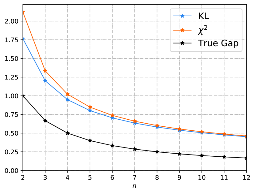
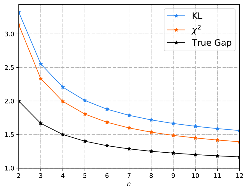
Estimate the Gaussian Mean. Consider the task of estimating the mean of Gaussian random variables. We assume the training sample comes from the distribution $\mathcal{N}(m,\sigma^{2})$, and the testing distribution is $\mathcal{N}(m^{\prime},(\sigma^{\prime})^{2})$. We define the loss function as $\ell\left(w,z\right)=(w-z)^{2}$, then the ERM algorithm yields the estimation $w=\frac{1}{n}\sum_{i=1}^{n}z_{i}$. See Appendix C-A for more details. Under the above settings, the loss function is sub-Gaussian with parameter $2((\sigma^{\prime})^{2}+\sigma^{2}/n)$, and thus Corollary 4 and Corollary 21 apply. The known KL-bounds and the newly derived $\chi^{2}$-bounds are compared in Fig. 1(a) and Fig. 1(b), where we set $(m,\sigma^{2})=(1,1)$. In Fig. 1(a) the two bounds are compared under the in-distribution setting, i.e., $m^{\prime}=m$ and $\sigma^{\prime}=\sigma$. A rigorous analysis shows that both $\chi^{2}$- and KL-bound decay at the rate $\mathcal{O}(1/\sqrt{n})$, while the true generalization gap decays at the rate $\mathcal{O}(1/n)$. Moreover, the KL-bound has the form of $c\sqrt{\log(1+\frac{1}{n})}$ while the $\chi^{2}$-bound has the form of $c\sqrt{1/n}$. Thus the KL-bound is tighter than the $\chi^{2}$-bound and they are asymptotically equivalent as $n\to\infty$. On the other hand, We compare the OOD case in Fig. 1(b), where we set $m^{\prime}=1$ and $(\sigma^{\prime})^{2}=2$. We observe that the $\chi^{2}$-bound is tighter than the KL-bound at the every beginning. By comparing the $\chi^{2}$-bound (20) and the KL-bound (18), we conclude that the $\chi^{2}$-bound will be tighter than the KL-bound whenever $\chi^{2}\left(P_{i}||Q\right)<2D_{\mathrm{KL}}\left(P_{i}||Q\right)$, since the variance of a random variable is no more than its sub-Gaussian parameter.

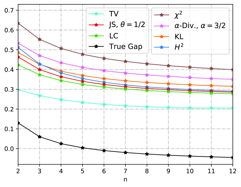
Estimate the Bernoulli Mean. Consider the previous example where the Gaussian distribution is replaced with the Bernoulli distribution. We assume the training samples are generated from the distribution $(\mathrm{Bern}(p))^{\otimes n}$ and the test data follows $\mathrm{Bern}(p^{\prime})$. Again we define the loss function as $\ell\left(w,z\right)=(w-z)^{2}$ and choose the estimation $w=\frac{1}{n}\sum_{i=1}^{n}z_{i}$. See Appendix C-B for more details.

Under the above settings, the loss function is bounded with $B=1$. Most of the generalization bounds derived in Section IV are given in Fig. 1(c), where $p=0.3$ and $p^{\prime}$ is set to $0.1$. In this case, we see that the squared Hellinger, Jensen-Shannon, and Le Cam bounds are tighter than the KL-bound. In Appendix C-B we also provide an example where $\chi^{2}$- and $\alpha$-divergence bounds are tighter than the KL-bound. But all these $f$-divergence-type generalization bounds are looser than the total variation bound, as illustrated by (24).

References

  • [1] V. Vapnik and A. Y. Chervonenkis, “On the uniform convergence of relative frequencies of events to their probabilities,” Theory of Probability & Its Applications, vol. 16, no. 2, pp. 264–280, 1971.
  • [2] P. L. Bartlett and S. Mendelson, “Rademacher and gaussian complexities: Risk bounds and structural results,” Journal of Machine Learning Research, vol. 3, no. Nov, pp. 463–482, 2002.
  • [3] D. Pollard, Convergence of stochastic processes.   David Pollard, 1984.
  • [4] O. Bousquet and A. Elisseeff, “Stability and generalization,” The Journal of Machine Learning Research, vol. 2, pp. 499–526, 2002.
  • [5] D. A. McAllester, “Some pac-bayesian theorems,” in Proceedings of the eleventh annual conference on Computational learning theory, 1998, pp. 230–234.
  • [6] D. Russo and J. Zou, “Controlling bias in adaptive data analysis using information theory,” in Artificial Intelligence and Statistics.   PMLR, 2016, pp. 1232–1240.
  • [7] A. Xu and M. Raginsky, “Information-theoretic analysis of generalization capability of learning algorithms,” Advances in Neural Information Processing Systems, vol. 30, 2017.
  • [8] Y. Bu, S. Zou, and V. V. Veeravalli, “Tightening mutual information-based bounds on generalization error,” IEEE Journal on Selected Areas in Information Theory, vol. 1, no. 1, pp. 121–130, 2020.
  • [9] T. Steinke and L. Zakynthinou, “Reasoning about generalization via conditional mutual information,” in Conference on Learning Theory.   PMLR, 2020, pp. 3437–3452.
  • [10] M. Haghifam, J. Negrea, A. Khisti, D. M. Roy, and G. K. Dziugaite, “Sharpened generalization bounds based on conditional mutual information and an application to noisy, iterative algorithms,” Advances in Neural Information Processing Systems, vol. 33, pp. 9925–9935, 2020.
  • [11] F. Hellström and G. Durisi, “Generalization bounds via information density and conditional information density,” IEEE Journal on Selected Areas in Information Theory, vol. 1, no. 3, pp. 824–839, 2020.
  • [12] J. Negrea, M. Haghifam, G. K. Dziugaite, A. Khisti, and D. M. Roy, “Information-theoretic generalization bounds for sgld via data-dependent estimates,” Advances in Neural Information Processing Systems, vol. 32, 2019.
  • [13] B. Rodríguez-Gálvez, G. Bassi, R. Thobaben, and M. Skoglund, “On random subset generalization error bounds and the stochastic gradient langevin dynamics algorithm,” in 2020 IEEE Information Theory Workshop (ITW).   IEEE, 2021, pp. 1–5.
  • [14] R. Zhou, C. Tian, and T. Liu, “Individually conditional individual mutual information bound on generalization error,” IEEE Transactions on Information Theory, vol. 68, no. 5, pp. 3304–3316, 2022.
  • [15] M. Arjovsky, L. Bottou, I. Gulrajani, and D. Lopez-Paz, “Invariant risk minimization,” arXiv preprint arXiv:1907.02893, 2019.
  • [16] X. Wu, J. H. Manton, U. Aickelin, and J. Zhu, “Information-theoretic analysis for transfer learning,” in 2020 IEEE International Symposium on Information Theory (ISIT).   IEEE, 2020, pp. 2819–2824.
  • [17] M. S. Masiha, A. Gohari, M. H. Yassaee, and M. R. Aref, “Learning under distribution mismatch and model misspecification,” in 2021 IEEE International Symposium on Information Theory (ISIT).   IEEE, 2021, pp. 2912–2917.
  • [18] Z. Wang and Y. Mao, “Information-theoretic analysis of unsupervised domain adaptation,” arXiv preprint arXiv:2210.00706, 2022.
  • [19] A. R. Esposito, M. Gastpar, and I. Issa, “Generalization error bounds via rényi-, f-divergences and maximal leakage,” IEEE Transactions on Information Theory, vol. 67, no. 8, pp. 4986–5004, 2021.
  • [20] G. Lugosi and G. Neu, “Generalization bounds via convex analysis,” in Conference on Learning Theory.   PMLR, 2022, pp. 3524–3546.
  • [21] Y. Polyanskiy and Y. Wu, “Information theory: From coding to learning,” Book draft, 2022.
  • [22] J. Birrell, P. Dupuis, M. A. Katsoulakis, Y. Pantazis, and L. Rey-Bellet, “(f, $\gamma$)-divergences: interpolating between f-divergences and integral probability metrics,” The Journal of Machine Learning Research, vol. 23, no. 1, pp. 1816–1885, 2022.
  • [23] R. Agrawal and T. Horel, “Optimal bounds between f-divergences and integral probability metrics,” The Journal of Machine Learning Research, vol. 22, no. 1, pp. 5662–5720, 2021.
  • [24] A. Müller, “Integral probability metrics and their generating classes of functions,” Advances in applied probability, vol. 29, no. 2, pp. 429–443, 1997.
  • [25] M. Raginsky, A. Rakhlin, M. Tsao, Y. Wu, and A. Xu, “Information-theoretic analysis of stability and bias of learning algorithms,” in 2016 IEEE Information Theory Workshop (ITW).   IEEE, 2016, pp. 26–30.
  • [26] V. Feldman and T. Steinke, “Calibrating noise to variance in adaptive data analysis,” in Conference On Learning Theory.   PMLR, 2018, pp. 535–544.
  • [27] S. Boucheron, G. Lugosi, and P. Massart, “Concentration inequalities: A nonasymptotic theory of independence. univ. press,” 2013.

Appendix A Proof of Section III

A-A Proof of Proposition 11

The proof relies on the variational representation of $f$-divergence as presented in the following lemma.

Lemma 2 (Variational Representation of $f$-Divergence [21]).
$$D_{f}\left(P||Q\right)=\sup_{g}\bigl{\{}\mathbb{E}_{P}\left[g\right]-\Lambda_{f;Q}\left(g\right)\bigr{\}},$$ (27)

where the supreme can be either taken over

  1. 1.

    the set of all simple functions, or

  2. 2.

    $\mathcal{M}(\mathcal{X})$, the set of all measurable functions, or

  3. 3.

    $L_{Q}^{\infty}(\mathcal{X})$, the set of all $Q$-almost-surely bounded functions.

In particular, we recover the Donsker-Varadhan variational representation of KL-divergence by combining Remark 2 and Lemma 2:

$$D_{\mathrm{KL}}\left(P||Q\right)=\sup_{g}\bigl{\{}\mathbb{E}_{P}\left[g\right]-\log\mathbb{E}_{Q}\left[e^{g}\right]\bigr{\}}.$$ (28)
Proof of Proposition 11.

We notice that if $F^{*}$ is the Legendre dual of some functional $F:\mathcal{X}\to\mathbb{R}$, then we have

$$(tF)^{*}(x^{*})=tF^{*}\left(\frac{1}{t}x^{*}\right),$$ (29)

for all $t\in\mathbb{R}_{+}$ and $x^{*}\in\mathcal{X}^{*}$, the dual space of $\mathcal{X}$. Let $Q$ be a fixed reference distribution, $\eta$ be a probability distribution, and $g$ be a measurable function. Combining the above fact with Lemma 2 yields the following Fenchel-Young inequality:

$$\mathbb{E}_{\eta}\left[g\right]\leq\frac{1}{t}D_{f}\left(\eta||Q\right)+\frac{1}{t}\Lambda_{f;Q}\left(tg\right),t\in\mathbb{R}_{+}.$$ (30)

As a consequence, we have

$\displaystyle\quad\ \mathrm{gen}\left(P_{W|Z^{n}},\nu,\mu\right)$
$\displaystyle=\mathbb{E}_{P_{W|Z^{n}}\otimes\nu^{\otimes n}}\left[\mathbb{E}_{\mu}\left[\ell\left(W,Z\right)\right]-\frac{1}{n}\sum_{i=1}^{n}\ell\left(W,Z_{i}\right)\right]$ (31)
$\displaystyle=\frac{1}{n}\sum_{i=1}^{n}\mathbb{E}_{P_{i}}\left[\bar{\ell}\left(W,Z_{i}\right)\right]$ (32)
$\displaystyle\leq\frac{1}{n}\sum_{i=1}^{n}\mathbb{E}_{P_{i}}\left[\bar{\ell}\left(W,Z_{i}\right)\right]-\mathbb{E}_{\eta_{i}}\left[\bar{\ell}\left(W,Z_{i}\right)\right]$
$\displaystyle+\frac{1}{t_{i}}\Bigl{(}D_{f}\left(\eta_{i}||Q\right)+\Lambda_{f;Q}\left(t_{i}\bar{\ell}\left(W,Z_{i}\right)\right)\Bigr{)}$ (33)
$\displaystyle\leq\frac{1}{n}\sum_{i=1}^{n}\sup_{g\in\bar{\Gamma}}\bigl{\{}\mathbb{E}_{P_{i}}\left[g\right]-\mathbb{E}_{\eta_{i}}\left[g\right]\bigr{\}}$
$\displaystyle+\frac{1}{t_{i}}\Bigl{(}D_{f}\left(\eta_{i}||Q\right)+\Lambda_{f;Q}\left(t_{i}\bar{\ell}\left(W,Z_{i}\right)\right)\Bigr{)}$ (34)
=RHS of(11).absentRHS ofitalic-(11italic-)\displaystyle=\text{RHS of}~{}\eqref{equation::fundamental inequality}. (35)

Here, inequality (33) follows from (30) and inequality (34) follows since $\bar{\ell}\in\bar{\Gamma}$, and equality (35) follows by Definition 8. ∎

We provide an alternative proof of Proposition 11, demonstrating its relationship with $(f,\Gamma)$-divergence [22]. We start with its definition.

Definition 4 ($(f,\Gamma)$-Divergence [22]).

Let $\mathcal{X}$ be a probability space. Suppose $P,Q\in\mathcal{P}(\mathcal{X})$ and $\Gamma\subseteq\mathcal{M}(\mathcal{X})$, $f$ be the convex function that induces the $f$-divergence. The $(f,\Gamma)$-divergence between distribution $P$ and $Q$ is defined by

$$D_{f}^{\Gamma}\left(P||Q\right)\coloneq\sup_{g\in\Gamma}\bigl{\{}\mathbb{E}_{P}\left[g\right]-\Lambda_{f;Q}\left(g\right)\bigr{\}}.$$ (36)

The $(f,\Gamma)$-divergence admits an upper bound, which interpolates between $\Gamma$-IPM and $f$-divergence.

Lemma 3.

(​[22, Theorem 8])

$$D_{f}^{\Gamma}\left(P||Q\right)\leq\inf_{\eta\in\mathcal{P}(\mathcal{X})}\left\{W^{\Gamma}\left(P,\eta\right)+D_{f}\left(\eta||Q\right)\right\}.$$ (37)

Now we are ready to prove Proposition 11.

Proof of Proposition 11 using $(f,\Gamma)$-Divergence.
$\displaystyle\quad\ \mathrm{gen}\left(P_{W|Z^{n}},\nu,\mu\right)=\frac{1}{n}\sum_{i=1}^{n}\mathbb{E}_{P_{i}}\left[\bar{\ell}\left(W,Z_{i}\right)\right]$ (38)
$\displaystyle=\frac{1}{n}\sum_{i=1}^{n}\frac{1}{t_{i}}\mathbb{E}_{P_{i}}\left[t_{i}\bar{\ell}\left(W,Z_{i}\right)\right]$ (39)
$\displaystyle\leq\frac{1}{n}\sum_{i=1}^{n}\frac{1}{t_{i}}\left(D_{f}^{t_{i}\bar{\Gamma}}\left(P_{i}||Q\right)+\Lambda_{f;Q}\left(t_{i}\bar{\ell}\left(W,Z_{i}\right)\right)\right)$ (40)
$\displaystyle\leq\frac{1}{n}\sum_{i=1}^{n}\frac{1}{t_{i}}\inf_{\eta_{i}\in\mathcal{P}\left(\mathcal{W}\times\mathcal{Z}\right)}\Bigl{\{}W^{t_{i}\bar{\Gamma}}\left(P_{i},\eta_{i}\right)$
$\displaystyle+D_{f}\left(\eta_{i}||Q\right)+\Lambda_{f;Q}\left(t_{i}\bar{\ell}\left(W,Z_{i}\right)\right)\Bigr{\}}$ (41)
=RHS of(11).absentRHS ofitalic-(11italic-)\displaystyle=\text{RHS of}~{}\eqref{equation::fundamental inequality}. (42)

Here equality (38) follows by (32), inequality (40) follows by Definition 36 and the condition $t_{i}\bar{\ell}\in t_{i}\bar{\Gamma}$, inequality (41) follows by Lemma 37, and equality (42) follows by the fact that $\dfrac{1}{t}W^{t\bar{\Gamma}}\left(P_{i},\eta_{i}\right)=W^{\bar{\Gamma}}\left(P_{i},\eta_{i}\right)$, for all $t\in\mathbb{R}_{+}$. ∎

A-B Tightness of the Proposition 11

The following proposition says that the equality in Proposition 11 can be achieved under certain conditions.

Proposition 2.

The upper bound in Proposition 11 achieves equality if the following two conditions hold simultaneously.

  1. 1.

    $\bar{\Gamma}$ is a singleton, i.e., $\bar{\ell}$ is the only element of $\bar{\Gamma}$.

  2. 2.

    For each $i=1,\ldots,n$, the distribution $\eta_{i}$ and the parameter $t_{i}$ are related through

    $$\mathrm{d}\eta_{i}/\mathrm{d}Q=(f^{*})^{\prime}\left(t_{i}\bar{\ell}\left(w,z\right)-\lambda_{i}\right),$$ (43)

    where $\lambda_{i}\in\mathbb{R}$ makes (43) a probability density:

    $$\mathbb{E}_{Q}\left[(f^{*})^{\prime}\left(t_{i}\bar{\ell}\left(W,Z\right)-\lambda_{i}\right)\right]=1.$$ (44)
Remark 4.

Under the case of KL-divergence (see Remark 2), we have $(f^{*})^{\prime}(x)=e^{x}$ and thus $\lambda_{i}=\log\mathbb{E}_{Q}\left[e^{t_{i}\bar{\ell}(W,Z)}\right]$. Therefore, the optimal $\eta_{i}$ has the form of

$$\mathrm{d}\eta_{i}/\mathrm{d}Q(w,z)=\frac{e^{t_{i}\bar{\ell}(w,z)}}{\mathbb{E}_{Q}\left[e^{t_{i}\bar{\ell}(W,Z)}\right]}=\frac{e^{-t_{i}\ell(w,z)}}{\mathbb{E}_{Q}\left[e^{-t_{i}\ell(W,Z)}\right]}.$$ (45)

This means that the optimal $\eta_{i}$ is achieved exactly at the Gibbs posterior distribution, with $t_{i}$ acting as the inverse temperature.

Proof of Proposition 2.

By assumption 1, we have $W^{\bar{\Gamma}}\left(P_{i},\eta_{i}\right)=\mathbb{E}_{P_{i}}\left[\bar{\ell}\right]-\mathbb{E}_{\eta_{i}}\left[\bar{\ell}\right]$, and thus Proposition 11 becomes

$$\mathrm{gen}\left(P_{W|Z^{n}},\nu,\mu\right)\leq\frac{1}{n}\sum_{i=1}^{n}\Bigl{(}\mathbb{E}_{P_{i}}\left[\bar{\ell}\right]-\mathbb{E}_{\eta_{i}}\left[\bar{\ell}\right]\\ +\frac{1}{t_{i}}D_{f}\left(\eta_{i}||Q\right)+\frac{1}{t_{i}}\Lambda_{f;Q}\left(t_{i}\bar{\ell}\left(W,Z\right)\right)\Bigr{)}.$$ (46)

As a consequence, it suffices to prove

$$\mathbb{E}_{\eta}\left[g\right]=\frac{1}{t}D_{f}\left(\eta||Q\right)+\frac{1}{t}\Lambda_{f;Q}\left(tg\right),$$ (47)

under the conditions that

$\displaystyle\mathrm{d}\eta/\mathrm{d}Q=(f^{*})^{\prime}\left(t(g-\lambda)\right),$ (48a)
$\displaystyle\mathbb{E}_{Q}\left[(f^{*})^{\prime}\left(t(g-\lambda)\right)\right]=1,$ (48b)

where $\eta,Q\in\mathcal{P}(\mathcal{X})$, $g\in\mathcal{M}(\mathcal{X})$, and $t\in\mathbb{R}_{+}$. If it is the case, then Proposition 2 follows by setting $\mathcal{X}=\mathcal{W}\times\mathcal{Z}$, $\eta=\eta_{i}$, $t=t_{i}$, $g=\bar{\ell}$, and $\lambda=\frac{1}{t_{i}}\lambda_{i}$. To see (47) holds, we need the following lemma

Lemma 4.

([22, Lemma 48])

$$f\bigl{(}(f^{*})^{\prime}(y)\bigr{)}=y(f^{*})^{\prime}(y)-f^{*}(y).$$ (49)

Then the subsequent argument is very similar to that of [22, Theorem 82]. We have

$\displaystyle\quad\ \sup_{P\in\mathcal{P}(\mathcal{X})}\Bigl{\{}\mathbb{E}_{P}\left[g\right]-\frac{1}{t}D_{f}\left(P||Q\right)\Bigr{\}}$ (50)
$\displaystyle\geq\lambda+\mathbb{E}_{\eta}\left[g-\lambda\right]-\frac{1}{t}D_{f}\left(\eta||Q\right)$ (51)
$\displaystyle=\lambda+\mathbb{E}_{Q}\left[(f^{*})^{\prime}(t(g-\lambda))(g-\lambda)\right]-\frac{1}{t}D_{f}\left(\eta||Q\right)$ (52)
$\displaystyle=\frac{1}{t}\bigl{(}t\lambda+\mathbb{E}_{Q}\left[f^{*}(t(g-\lambda))\right]\bigr{)}$ (53)
$\displaystyle\geq\frac{1}{t}\Lambda_{f;Q}\left(tg\right)$ (54)
$\displaystyle=\sup_{P\in\mathcal{P}(\mathcal{X})}\Bigl{\{}\mathbb{E}_{P}\left[g\right]-\frac{1}{t}D_{f}\left(P||Q\right)\Bigr{\}}.$ (55)

In the above, equality (52) follows by (48a), equality (53) follows by Lemma 49, inequality (54) follows by Definition 7, and equality (55) follows by Lemma 2 and equality (29). Therefore, all the inequalities above achieve the equality. This proves (47). ∎

A-C Proof of Theorem 12

We first invoke a key lemma.

Lemma 5 (Lemma 2.4 in [27]).

Let $\psi$ be a convex and continuously differentiable function defined on the interval $[0,b)$, where $0<b\leq+\infty$. Assume that $\psi(0)=\psi^{\prime}(0)=0$ and for every $t\geq 0$, let $\psi^{*}(t)=\sup_{\lambda\in(0,b)}\left\{\lambda t-\psi(\lambda)\right\}$ be the Legendre dual of $\psi$. Then the generalized inverse of $\psi^{*}$, defined by $\left(\psi^{*}\right)^{-1}(y)\coloneq\inf\left\{t\geq 0:\psi^{*}(t)>y\right\}$, can also be written as

$$\left(\psi^{*}\right)^{-1}(y)=\inf_{\lambda\in(0,b)}\frac{y+\psi(\lambda)}{\lambda}.$$ (56)
Proof of Theorem 12.

As a consequence of Lemma 56, we have

$\displaystyle\quad\ \mathrm{gen}\left(P_{W|Z^{n}},\nu,\mu\right)$
$\displaystyle\leq\frac{1}{n}\sum_{i=1}^{n}\inf_{\eta_{i}\in\mathcal{P}(\mathcal{W}\times\mathcal{Z}),\;t_{i}\in\mathbb{R}_{+}}\Bigl{\{}W^{\bar{\Gamma}}\left(P_{i},\eta_{i}\right)$
$\displaystyle+\frac{1}{t_{i}}D_{f}\left(\eta_{i}||Q\right)+\frac{1}{t_{i}}\Lambda_{f;Q}\left(t_{i}\bar{\ell}\left(W,Z\right)\right)\Bigr{\}}$ (57)
$\displaystyle\leq\frac{1}{n}\sum_{i=1}^{n}\inf_{\eta_{i}}\inf_{t_{i}}\biggl{\{}W^{\bar{\Gamma}}\left(P_{i},\eta_{i}\right)+\frac{D_{f}\left(\eta_{i}||Q\right)+\psi(t_{i})}{t_{i}}\biggr{\}}$ (58)
=RHS of (LABEL:equation::the_general_theorem),absentRHS of LABEL:equation::the_general_theorem\displaystyle=\text{RHS of }(\ref{equation::the general theorem}),

where the first inequality follows by Proposition 11 and the last equality follows by Lemma 56. ∎

A-D Proof of Corollary 14

Proof.

By inequality (33), it suffices to prove

$$\mathbb{E}_{P_{i}}\left[\bar{\ell}\left(W,Z_{i}\right)\right]-\mathbb{E}_{\eta_{i}}\left[\bar{\ell}\left(W,Z_{i}\right)\right]\leq W^{\Gamma}\left(P_{i},\eta_{i}\right).$$ (59)

If so, (14) will follow by exploiting Lemma 56 and optimizing over $t_{i}$ in (33). Since $\eta_{i}\in\mathcal{C}\left(P_{W},\cdot\right)$, the left-hand side of (59) is exactly $(\mathbb{E}_{\eta_{i}}\left[\ell\right]-\mathbb{E}_{P_{i}}\left[\ell\right])$. Thus (59) follows by $\ell\in\Gamma$ and by the symmetry of $\Gamma$. ∎

Appendix B Proofs in Section IV

B-A Proof of Corollary 15

Proof.

By Corollary 14, we have

$\displaystyle\quad\ \mathrm{gen}\left(P_{W|Z^{n}},\nu,\mu\right)$
$\displaystyle\leq\frac{1}{n}\sum_{i=1}^{n}\sup_{g\in\Gamma}\bigl{\{}\mathbb{E}_{P_{i}}\left[g\right]-\mathbb{E}_{Q}\left[g\right]\bigr{\}}$ (60)
$\displaystyle=\frac{1}{n}\sum_{i=1}^{n}\sup_{g\in\Gamma}\bigl{\{}\mathbb{E}_{P_{i}}\left[g\right]-\mathbb{E}_{P_{W}\otimes\nu}\left[g\right]+\mathbb{E}_{P_{W}\otimes\nu}\left[g\right]-\mathbb{E}_{Q}\left[g\right]\bigr{\}}$ (61)
$\displaystyle\leq\frac{1}{n}\sum_{i=1}^{n}\sup_{g\in\Gamma}\Bigl{\{}\mathbb{E}_{\nu}\left[\mathbb{E}_{P_{W|Z_{i}}}\left[g\right]-\mathbb{E}_{P_{W}}\left[g\right]\right]$
$\displaystyle+\mathbb{E}_{P_{W}}\left[\mathbb{E}_{\nu}\left[g\right]-\mathbb{E}_{\mu}\left[g\right]\right]\Bigr{\}}\qquad$ (62)
$\displaystyle\leq\frac{1}{n}\sum_{i=1}^{n}\mathbb{E}_{\nu}\left[L_{W}W_{1}(P_{W|Z_{i}},P_{W})\right]+L_{Z}W_{1}(\nu,\mu).$ (63)

In the above, inequality (62) follows by the tower property of conditional expectation, and inequality (63) follows by the Kantorovich-Rubinstein duality (10). ∎

B-B Proof of Corollary 3

Proof.

By assumption we have $\ell\in\Gamma$ and thus

$\displaystyle\mathrm{gen}\left(P_{W|Z^{n}},\nu,\mu\right)$ $\displaystyle\leq\frac{1}{n}\sum_{i=1}^{n}W^{\Gamma}\left(P_{i},Q\right)$ (64)
$\displaystyle=\frac{1}{n}\sum_{i=1}^{n}W^{\Gamma-B/2}(P_{i},Q)$ (65)
$\displaystyle=\frac{B}{n}\sum_{i=1}^{n}\mathrm{TV}\left(P_{i},Q\right).$ (66)

In the above, inequality (64) follows by Corollary 14, equality (65) follows by the translation invariance of IPM, and equality (66) follows by the variational representation of total variation:

$$\mathrm{TV}\left(P,Q\right)=\sup_{\|g\|_{\infty}\leq\frac{1}{2}}\bigl{\{}\mathbb{E}_{P}\left[g\right]-\mathbb{E}_{Q}\left[g\right]\bigr{\}}.$$ (67)

Thus we proved (16). Then (17) follows by the chain rule of total variation. The general form of the chain rule of total variation is given by

$$\mathrm{TV}\left(P_{X^{m}},Q_{X^{m}}\right)\leq\sum_{i=1}^{m}\mathbb{E}_{P_{X^{i-1}}}\left[\mathrm{TV}\left(P_{X_{i}|X^{i-1}},Q_{X_{i}|X^{i-1}}\right)\right].$$ (68)

B-C Proof of Corollaries 4 and 19

Proof.

It suffices to prove Corollary 4 and then Corollary 19 follows by a similar argument. By Theorem 12, we have

$\displaystyle\mathrm{gen}\left(P_{W|Z^{n}},\nu,\mu\right)\leq\frac{1}{n}\sum_{i=1}^{n}\sqrt{2\sigma^{2}D_{\mathrm{KL}}\left(P_{i}||Q\right)}$ (69)
$\displaystyle=\frac{1}{n}\sum_{i=1}^{n}\sqrt{2\sigma^{2}\bigl{(}D_{\mathrm{KL}}\left(P_{W|Z_{i}}||Q_{W}|\nu\right)+D_{\mathrm{KL}}\left(\nu||\mu\right)\bigr{)}},$ (70)

where the equality follows from the chain rule of KL divergence. Taking infimum over $Q_{W}$ yields (18), which is due to the following lemma.

Lemma 6 (Theorem 4.1 in [21]).

Suppose $(W,Z)$ is a pair of random variables with marginal distribution $P_{W}$ and let $Q_{W}$ be an arbitrary distribution of $W$. If $D_{\mathrm{KL}}\left(P_{W}||Q_{W}\right)<\infty$, then

$$I(W;Z)=D_{\mathrm{KL}}\left(P_{W|Z}||Q_{W}|Z\right)-D_{\mathrm{KL}}\left(P_{W}||Q_{W}\right).$$ (71)

Therefore, by the non-negativity of KL divergence, the infimum is achieved at $Q_{W}=P_{W}$ and thus $I(W;Z_{i})=D_{\mathrm{KL}}\left(P_{W|Z_{i}}||P_{W}|\nu\right)$. ∎

B-D Proof of Corollary 21

Proof.

A direct calculation shows $f^{*}(y)=\frac{1}{4}y^{2}+y$ for $f(x)=(x-1)^{2}$, and thus $\Lambda_{f;\mu}\left(t\bar{\ell}(w,Z)\right)=\frac{1}{4}\mathrm{Var}_{\mu}\ell\left(w,Z\right)t^{2}$. Therefore, we can choose $\psi(t)=\frac{1}{4}\sigma^{2}t^{2}$ and thus $(\psi^{*})^{-1}(y)=\sqrt{\sigma^{2}y}$. Applying Theorem 12 yields (20). ∎

B-E Proof of Corollary 7

Thanks to the Lemma 1, the proof can be condensed into Table III.

TABLE III: Comparison Between $f$-Divergences
$f$-Divergence $f(x)$ Condition (22) holds?
$\alpha$-Divergence $\dfrac{x^{\alpha}-\alpha x+\alpha-1}{\alpha(\alpha-1)}$ Only for $\alpha\in[-1,2]$
$\chi^{2}$-Divergence $(x-1)^{2}$ Yes
KL-Divergence $x\log x-(x-1)$ Yes
Squared Hellinger $(\sqrt{x}-1)^{2}$ Yes
Reversed KL $-\log x+x-1$ Yes
Jensen-Shannon(with parameter $\theta$) $\theta x\log x-(\theta x+1-\theta)\log(\theta x+1-\theta)$ Yes
Le Cam $\dfrac{1-x}{2(1+x)}+\dfrac{1}{4}(x-1)$ Yes
  • 1

    All the $f$ in Table (III) are all set to be standard, i.e., $f^{\prime}(1)=f(1)=0$.

  • 2

    Both the $\chi^{2}$-divergence and the squared Hellinger divergence are $\alpha$-divergence, up to a multiplicative constant. In particular, we have $\chi^{2}=2D_{2}$ and $H^{2}=\frac{1}{2}D_{1/2}$. The $\theta$-Jensen-Shannon divergence has the form of $D_{\mathrm{JS}(\theta)}(P||Q)=\theta D_{\mathrm{KL}}\left(P||R(\theta)\right)+(1-\theta)D_{\mathrm{KL}}\left(Q||R(\theta)\right)$, where $R(\theta)\coloneq\theta P+(1-\theta)Q$ and $\theta\in(0,1)$. The classical Jensen-Shannon divergence corresponds to $\theta=1/2$.

B-F Proof of Corollary 25

Proof.

Since $\bar{\Gamma}=\{\bar{\ell}\}$, we have

$\displaystyle W^{\bar{\Gamma}}\left(P_{i},\eta_{i}\right)$ $\displaystyle=\mathbb{E}_{P_{i}}\left[\bar{\ell}\right]-\mathbb{E}_{\eta_{i}}\left[\bar{\ell}\right]$ (72)
$\displaystyle=\mathbb{E}_{P_{W}\otimes\nu}\left[\ell\right]-\mathbb{E}_{P_{W|Z_{i}}\otimes\nu}\left[\ell\right].$ (73)

Inserting (73) into Theorem 12 and rearranging terms yields

$\displaystyle\quad\ \mathbb{E}_{P_{W}\otimes\mu}\left[\ell\right]-\mathbb{E}_{P_{W}\otimes\nu}\left[\ell\right]$
$\displaystyle\leq(\psi^{*})^{-1}(D_{f}\left(P_{W}\otimes\nu||P_{W}\otimes\mu\right))$ (74)
$\displaystyle=(\psi^{*})^{-1}(D_{f}\left(\nu||\mu\right)).$ (75)

Appendix C Supplementary materials of Section V

C-A Details of Estimating the Gaussian Means

To calculate the generalization bounds we need the distribution $P_{i}$ and $Q$. All the following results are given in the general $d$-dimensional case, where we let the training distribution be $\mathcal{N}(\mathbf{m},\sigma^{2}\mathbf{I}_{d})$ and the testing distribution be $\mathcal{N}(\mathbf{m}^{\prime},(\sigma^{\prime})^{2}\mathbf{I}_{d})$. Our example corresponds to the special case $d=1$.

We can check that both $P_{i}$ and $Q$ are joint Gaussian. Write the random vector as $\displaystyle[\mathbf{Z}^{\mathrm{T}},\mathbf{W}^{\mathrm{T}}]^{\mathrm{T}}$, then $P_{i}$ and $Q$ are given by

$\displaystyle P_{i}=\mathcal{N}\left(\left[\begin{array}[]{cc}\mathbf{m}\\[4.0pt] \mathbf{m}\end{array}\right],\left[\begin{array}[]{cc}\sigma^{2}\mathbf{I}_{d},&\frac{1}{n}\sigma^{2}\mathbf{I}_{d}\\[4.0pt] \frac{1}{n}\sigma^{2}\mathbf{I}_{d},&\frac{1}{n}\sigma^{2}\mathbf{I}_{d}\end{array}\right]\right),$ (80)
$\displaystyle Q=\mathcal{N}\left(\left[\begin{array}[]{cc}\mathbf{m}^{\prime}\\[2.0pt] \mathbf{m}\end{array}\right],\left[\begin{array}[]{cc}(\sigma^{\prime})^{2}\mathbf{I}_{d},&\mathbf{0}\\[2.0pt] \mathbf{0},&\frac{1}{n}\sigma^{2}\mathbf{I}_{d}\end{array}\right]\right).$ (85)

The KL divergence between $P_{i}$ and $Q$ is given by

$$D_{\mathrm{KL}}\left(P_{i}||Q\right)=\log\frac{\det\mathbf{\Sigma}_{P_{i}}}{\det\mathbf{\Sigma}_{Q}}-2d+\mathrm{Tr}(\mathbf{\Sigma}_{P_{i}}\mathbf{\Sigma}_{Q}^{-1})\\ +\exp\bigl{(}(\mathbf{m}_{P_{i}}-\mathbf{m}_{Q})^{\mathrm{T}}\mathbf{\Sigma}_{Q}^{-1}(\mathbf{m}_{P_{i}}-\mathbf{m}_{Q})\bigr{)},$$ (86)

where $\mathbf{m}_{P_{i}}$ (resp., $\mathbf{m}_{Q}$) denotes the mean vector of $P_{i}$ (resp., $Q$), and $\mathbf{\Sigma}_{P_{i}}$ (resp., $\mathbf{\Sigma}_{Q}$) denotes the covariance matrix of $P_{i}$ (resp., $Q$). The $\chi^{2}$ divergence between $P_{i}$ and $Q$ is given by

$$\chi^{2}\left(P_{i}||Q\right)=\frac{\det\mathbf{\Sigma}_{Q}}{\sqrt{\det\mathbf{\Sigma}_{P_{i}}}\sqrt{\det\bigl{(}2\mathbf{\Sigma}_{Q}-\mathbf{\Sigma}_{P_{i}}\bigr{)}}}\cdot\\ \exp\Bigl{(}(\mathbf{m}_{P_{i}}-\mathbf{m}_{Q})^{\mathrm{T}}\bigl{(}2\mathbf{\Sigma}_{Q}-\mathbf{\Sigma}_{P}\bigr{)}^{-1}(\mathbf{m}_{P_{i}}-\mathbf{m}_{Q})\Bigr{)}-1.$$ (87)

Finally, the true generalization gap is given by

$$\mathrm{gen}\left(P_{W|Z^{n}},\nu,\mu\right)=\left((\sigma^{\prime})^{2}-\sigma^{2}\right)d+\frac{2\sigma^{2}d}{n}+\|\mathbf{m}-\mathbf{m}^{\prime}\|_{2}^{2}.$$ (88)

C-B Details of Estimating the Bernoulli Means

A direct calculation shows

$$P_{i}\left(\begin{aligned} &Z_{i}=1\\ &W=\frac{k}{n}\end{aligned}\right)=\left\{\begin{aligned} &\binom{n-1}{k-1}p^{k}(1-p)^{n-k-1},1\leq k\leq n,\\ &0,k=0,\end{aligned}\right.$$ (89)
$$P_{i}\left(\begin{aligned} &Z_{i}=0\\ &W=\frac{k}{n}\end{aligned}\right)=\left\{\begin{aligned} &\binom{n-1}{k}p^{k}(1-p)^{n-k},0\leq k\leq n-1,\\ &0,k=n.\end{aligned}\right.$$ (90)

The distribution $Q$ is the product of $\mathrm{Bern}(p^{\prime})$ and the binomial distribution with parameter $(n,p)$. Then the $f$-divergence can be directly calculated by definition. Finally, the true generalization gap is given by

$$\mathrm{gen}\left(P_{W|Z^{n}},\nu,\mu\right)=2\sum_{k=1}^{n}\binom{n-1}{k-1}p^{k}(1-p)^{n-1}\frac{k}{n}\\ +(1-2p)p^{\prime}-p.$$ (91)
Figure 2: Bernoulli, $p=0.3$, $p^{\prime}=0.5$.
Refer to caption
Figure 3: Bernoulli, $n=10$, $p=0.6$.
Refer to caption

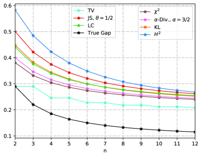
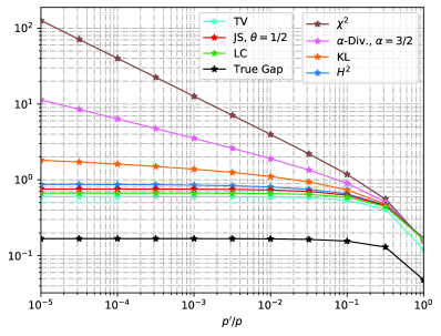
Supplementary results are given in Fig. 2 and Fig. 3. If we define the Hamming distance over the hypothesis space and the data space, then the total variation bound coincides with the Wasserstein distance bound. From Fig. 1(c) and Fig. 2 we observe that there exists a approximately monotone relationship between $\chi^{2}$-divergence, $\alpha$-divergence ($\alpha=3/2$), KL-divergence, and the squared Hellinger divergence. This is because all these bounds are $\alpha$-divergence type, with KL-divergence corresponds to $\alpha=1$444Strictly speaking, $D_{\mathrm{KL}}=R_{1}$, the Rényi-$\alpha$-divergence with $\alpha=1$, and $R_{\alpha}$ is a $\log$-transformation of the $\alpha$-divergence.. Moreover, we observe that the Le Cam divergence is always tighter than the Jensen-Shannon divergence. This is because the generator $f$ of Le Cam is smaller than that of Jensen-Shannon, and they share the same coefficient $\sigma_{f}=1$.

We consider the extreme case in Fig. 3, where $n=10$, $p=0.6$, and we allow $p^{\prime}$ decays to 00. When $p^{\prime}$ is sufficiently small, the KL-bound (along with $\alpha$-divergence ($\alpha=3/2$) and $\chi^{2}$-bound) is larger than $1$ and thus becomes vacuous. While the squared Hellinger, Jensen-Shannon, Le Cam, and total variation bounds do not suffer such a problem.