Policy-Space Search:
Equivalences, Improvements, and Compression
Abstract
Fully-observable non-deterministic (FOND) planning is at the core of artificial intelligence planning with uncertainty. It models uncertainty through actions with non-deterministic effects. A∗ with Non-Determinism (AND∗) (Messa and Pereira, 2023) is a FOND planner that generalizes A∗ (Hart et al., 1968) for FOND planning. It searches for a solution policy by performing an explicit heuristic search on the policy space of the FOND task. In this paper, we study and improve the performance of the policy-space search performed by AND∗. We present a polynomial-time procedure that constructs a solution policy given just the set of states that should be mapped. This procedure, together with a better understanding of the structure of FOND policies, allows us to present three concepts of equivalences between policies. We use policy equivalences to prune part of the policy search space, making AND∗ substantially more effective in solving FOND tasks. We also study the impact of taking into account structural state-space symmetries to strengthen the detection of equivalence policies and the impact of performing the search with satisficing techniques. We apply a recent technique from the group theory literature to better compute structural state-space symmetries. Finally, we present a solution compressor that, given a policy defined over complete states, finds a policy that unambiguously represents it using the minimum number of partial states. AND∗ with the introduced techniques generates, on average, two orders of magnitude fewer policies to solve FOND tasks. These techniques allow explicit policy-space search to be competitive in terms of both coverage and solution compactness with other state-of-the-art FOND planners.
keywords:
FOND Planning , Equivalence Pruning , Structural Symmetries , Policy Compression , Heuristic Search[ufrgs]organization=Institute of Informatics, Federal University of Rio Grande do Sul, country=Brazil
1 Introduction
Fully-observable non-deterministic (FOND) planning models tasks with uncertainty through actions with non-deterministic effects. A solution for a FOND task is a policy that takes into account all the possible outcomes of each action and describes what actions should be taken in what states so that one, starting from the initial state, following its guidance, eventually reaches a goal state. Despite modeling uncertainty, we are not concerned with concrete probabilities in FOND planning.
A∗ with Non-Determinism (AND∗ for short) (Messa and Pereira, 2023) generalizes A∗ (Hart et al., 1968) for FOND planning. It explicitly searches for a solution policy in the space of policies of the FOND task. Starting with only the empty policy, which maps no state to no action, AND∗ uses a priority queue to keep track of a range of incomplete policies that are candidates to become a solution. It repeatedly chooses from the queue the most promising candidate policy until it finds one that is a solution. If the chosen policy is not yet a solution, AND∗ replaces it in the queue with its successor policies. AND∗ is sound and complete, and is able to find a solution with a minimal number of mapped states when using a suitable heuristic function to evaluate the promise of the candidate policies (Messa and Pereira, 2023).
In this work, we study policy equivalences. In the same way that two different solutions that have the same size can be considered equivalent, assuming we just want to optimize their compactness, we can have specific rules that determine whether two candidate policies are equivalent for the purposes of finding a (compact) solution. We study how to derive policy equivalence rules by looking at the structure of the policies. We use these rules to avoid expanding multiple policies from the same class of equivalence, substantially improving the performance of AND∗. We introduce a polynomial-time procedure, called the concretizer, that allows the construction of a solution policy by only knowing its states and not its mappings. This procedure allows the development of stronger rules of policy equivalences.
Similarly to how policies can be equivalent to one another, states can also be equivalent to one another. We detect equivalences of states through the computation of structural symmetries (Pochter et al., 2011; Shleyfman et al., 2015). And we use that to strengthen the detection of equivalent policies. We apply a recent technique from the group theory literature to improve the computation of structural symmetries.
Besides equivalence pruning, we study two other modifications to the search procedure that can improve its performance. We study the impact of early deadlock pruning on AND∗ with equivalence pruning, and we also verify the impact of performing the search using satisficing techniques, such as a greedy best-first policy-space search. We present two variants of AND∗: Weighted A∗ with Non-Determinism (WAND∗) and Greedy Best-First Search with Non-Determinism (GBFSND), which are analogous to Weighted A∗ (WA∗) (Pohl, 1970) and Greedy Best-First Search (GBFS) (Doran and Michie, 1966), for FOND planning.
Finally, we introduce a procedure, called the compressor, that allows the compression of solution policies found by any FOND planner using partial states. The compressor receives as input a policy defined over complete states and returns a policy defined over partial states that represents the same information, using the minimal number of partial states. The compressor is time and memory-efficient for the benchmark tasks we solve and makes the solutions returned by AND∗ have state-of-the-art compactness in the majority of the benchmark domains.
In this work, we start by presenting some background on FOND planning and policy-space search (Section 2). Then, we present the concept of search equivalence pruning and propose three different concepts of equivalences between policies, with different guarantees and effectiveness (Section 3). We proceed by presenting concepts of state equivalences and using them to strengthen the concepts of policy equivalences (Section 4). Then, we analyze the impact of early deadlock pruning and satisficing search techniques (Section 5). Finally, we present the solution compressor (Section 6), compare AND∗ with state-of-the-art FOND planners (Section 7), and conclude (Section 8). Formal theoretical proofs are presented in Appendix A and B. A helpful glossary of the main symbols and functions used in this work is presented in Appendix C.
2 Background on FOND Planning and Policy-Space Search
A FOND task , in STRIPS (Fikes and Nilsson, 1971) formalism, is a 4-tuple , with a finite set of facts that can be either true or false, the facts that are true in the initial state , the facts that we want to be true, i.e. the goal, and a finite set of actions. are the facts that are true in a state , and a state is a goal state iff . There are states, one for each truth valuation. We call the set of all possible states, and the set with all goal states.
Each action is a pair , with the precondition of and the effects of . An action can be applied to a state iff . Each of is a pair , with , and . The application of to a given state non-determinitically results in a state , with .
A transition is a triplet with a state, an action applicable to , and . The start of is and the end of is . And the action of is .
A trajectory is a sequence of transitions , with for each . The start of is and the end of is . If , then is any state.
A policy is a partial function mapping non-goal states to actions, with applicable to for each . A -trajectory is a trajectory , with for each . The reachability set of is . The frontier set of is . We call and . A policy is closed iff and goal-closed iff . A policy is proper iff for each . We note that if is proper, then each is proper as well. We call for . A policy that is simultaneously goal-closed and proper is called strong-cyclic.
A solution for is a strong-cyclic policy with . In other words, a solution is a policy that under a non-adversarial111Also called “fair environment”. (Cimatti et al., 2003) environment safely guides one from to a goal state, by addressing all the possible outcomes of the taken actions, although possibly visiting some states an arbitrary number of times before eventually reaching the goal, due to possible cyclic -trajectories. We call . The set captures if a policy is goal-closed and deals with the initial state. Specifically, iff is goal-closed and . Consequently, a proper policy is a solution iff. We remark that a simplified glossary of the symbols and functions we most use throughout this work is presented on the last page of this work (in Appendix C).
Figure 1 depicts the state space of a FOND task. It has six states – the initial state –, , , , , and – the single goal state; and six actions , , , , , and . The only non-deterministic actions are – which can lead to either or from – and – which can lead to either or from . We use it to exemplify some of the presented concepts regarding policies. is a strong-cyclic policy, meaning that it is goal-closed and proper. It is goal-closed because . It is proper because for each , , giving that there is a -trajectory leading to and another leading to . For instance, the -trajectories and respectively lead and to . It is true one may cycle an arbitrary number of times between and before reaching a solution if they follow actions starting from one of these states. However, the assumption of non-adversity ensures that the “incorrect” effect of will not occur forever and that the one leading them to will eventually occur. is not a solution because it does not cover the initial state (i.e. ). The only solution for this example task is . is a slice of . The policy is not a solution because it is not proper. It is not proper because and . This occurs because and . They form a deadlock. Differently from the cycle between and , the cycle formed by and in is inescapable because there is no effect that leads outside it.
2.1 Searching for a Solution
The A∗ with Non-Determinism (AND∗ for short) algorithm (Messa and Pereira, 2023) generalizes the A∗ algorithm (Hart et al., 1968) for FOND planning. It is a best-first heuristic search algorithm that uses a priority queue over policies to explore the policy space of and search for a solution policy. It starts with the empty policy . At each iteration, it removes from the priority queue a policy with lowest value and returns it if it is a solution for . Otherwise, AND∗ expands to generate successor222We note that there are alternative ways of defining the successors of a given policy . For instance, we could generate instead policies with mapping at once every state in to some action. That would result in a “big-step” successor function. Messa and Pereira (2023) discuss “big-step” vs. “small-step”. policies for some state and each action applicable to (given that there is one such state , otherwise is simply discarded). Each generated successor policy is inserted in the priority queue. If the priority queue becomes empty, then there is no solution for . Algorithm 1 shows the pseudocode for AND∗. AND∗ is sound and complete (Messa and Pereira, 2023).
When aiming to find a solution policy with minimal domain size, we say that the -value (already paid cost) of a policy is , and that the -value (remaining cost) of is the minimum such that is a solution for (or iff there is no such ). A heuristic function that estimates is admissible iff for each policy and is goal-aware iff for each solution . The values AND∗ uses to guide its search should evaluate how promising the candidate policy is. When using with an admissible and goal-aware heuristic function, AND∗ returns optimal solutions (with minimal domain size, in this case).
In this work, we use a slightly improved version (Equation 1) of admissible and goal-aware heuristic function (Messa and Pereira, 2023). is a heuristic that directly returns -values for policies, instead of -values. We use (Helmert and Domshlak, 2009) as the classical planning heuristic sub-component of .
| (1) |
| (2) |
We use Figure 1’s example to illustrate the computation of . Let . Note that , , and . Let . Then and . This means, by admissibility, that any solution has a size of at least five. If we set , we have .
2.2 Benchmarks and Experimental Settings
Throughout this work, we present improvements for AND∗ and evaluate them through empirical experiments.
We use the same two benchmarks as Pereira et al. (2022) for our experiments. IPC-FOND, with 379 tasks over 12 FOND planning domains from the International Planning Competition (IPC), and NEW-FOND, introduced by Geffner and Geffner (2018), with 211 tasks over five FOND planning domains. The NEW-FOND benchmark was developed to mislead FOND planners. It has tasks with a large number of trajectories that lead to goal states but are not part of any solution.
We remove the tasks without solution, namely 25 tasks from the first-responders domain. These tasks are trivial because the PRP’s (Muise et al., 2012) translator we use to parse PDDL files detects their unsolvability. Moreover, as in Messa and Pereira (2023), we merge the blocksworld-new and blocksworld-2 domains into a single domain called blocksworld-advanced, as they actually are equal domains. Table 1 shows the resulting 16 benchmark domains.
| Domain | ||
|---|---|---|
| IPC-FOND | acrobatics | 8 |
| beam-walk | 11 | |
| blocksworld-original | 30 | |
| blocksworld-advanced | 55 | |
| chain-of-rooms | 10 | |
| earth-observation | 40 | |
| elevators | 15 | |
| faults | 55 | |
| first-responders | 75 | |
| tireworld-triangle | 40 | |
| zenotravel | 15 | |
| NEW-FOND | doors | 15 |
| islands | 60 | |
| miner | 51 | |
| tireworld-spiky | 11 | |
| tireworld-truck | 74 |
We run the experiments on an AMD Ryzen 9 3900X, using limits of GB and minutes per task. We use greater -value () as the AND∗ policy-selection tie-breaker, and we always select to map the most recently added state when generating the successors of a policy . Additionally, we make AND∗ not distinguish two distinct goal states (i.e., in AND∗ perspective, all generated goal states are the same.). This can be seen as a trivial application of the concept of state symmetries. We will make used code and data publicly available.
Each batch of experiment results is usually presented in a pair of tables. The first table presents the ratio of tasks that were solved, failed by the time limit, or failed by the memory limit for each domain for each configuration. The second table presents – over the intersection of tasks solved by all configurations tested in the batch – the arithmetic means of the execution time, the number of generated policies, and the return solution size for each domain for each configuration. Both tables have an extra row aggregating the results from all domains. All domains have the same weight in the aggregation, independently of the number of (solved) tasks each has. We use arithmetic means to aggregate ratios and geometric means to aggregate other kinds of information to avoid giving more weight to hard domains.
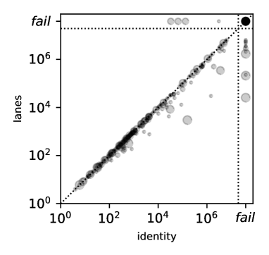
Additionally, we present scatter plot figures to visualize the reduction in the number of generated policies caused by each presented improvement. These figures have one mark for each task, with proportionally bigger marks for tasks from domains with fewer tasks.
3 Policy Equivalence Pruning
We can define a set of signatures and a function that maps policies to signatures in to define some concept of equivalence . We call iff . For example, if we define to be precisely the set of policies and to be the identity (i.e., ), then iff . The utility of a given concept of equivalence depends on its usage.
In classical planning, all actions are deterministic (). Therefore, a policy incrementally built from the initial state represents a single trajectory outgoing from it. Such a policy has with a size of either zero or one. If the size is zero, then the trajectory forms a cycle and is discarded. Thus, each relevant generated policy in classical planning has precisely one frontier state. If such a state is a goal state, then the policy is a solution (usually called a plan in classical planning literature). Otherwise, the state in is the new starting point from which we must find an outgoing trajectory to a goal state in order for the current policy to become a solution. Since the content of satisfactorily characterizes a policy regarding its potential to become a solution, we could then set , and333After this point, we refrain from explicitly defining the set of possible signatures when presenting a function. It will be assumed to be . . That would create a concept of equivalence among policies that would disregard their costs and consider equivalent two policies with the same set. Then, we can make the search algorithm discard a policy if another policy was previously considered. This is called equivalence pruning.
A common way to apply equivalence pruning is to store in a set the signatures of all policies previously removed from . Then, at the removal of a new policy , we can verify whether is or not in the set. If it is, then doesn’t need to be expanded and is discarded. Otherwise, is added to the set, and the algorithm proceeds ordinarily. Such a set is usually called in classical planning literature. We call it to avoid confusion with the policies property of “closedness”.
We note that using in classical planning is sound but does not ensure optimality as it considers solutions with different costs equivalent. Straightforwardly setting solves this problem. However, classical planning literature goes a step further. They use a reopening approach. With reopening, A∗ expands a policy iff or each previously expanded policy with had . This allows A∗ to be both sound and optimal with . The reopening approach can be seen as an asymmetrical pruning relation. Classical planning literature also shows that reopening is not required to ensure optimality when the used heuristic function has a consistency property (Edelkamp and Schrödl, 2011). In this work, we don’t apply reopening or define consistency for AND∗ but still determine whether optimality is ensured by default by each presented equivalence-pruning concept. Our main concerns are soundness, completeness, and empirical performance.
Algorithm 2 shows the pseudocode for AND∗ with equivalence pruning. Algorithm 1 is a special case of Algorithm 2 because they are equivalent when Algorithm 2’s is the identity (i.e., )444No policy is generated twice by AND∗ (Messa and Pereira, 2023).. Therefore, we hereafter refer to Algorithm 2 when we mention AND∗. AND∗ with is sound, complete, and – when using an admissible and goal-aware heuristic – optimal (Theorem 1, in A.2.1).
Since using is the same as not having equivalence pruning, we would like to have a better concept of equivalence than identity. Can we set like in classical planning? We use an example state space (depicted in Figure 2) to analyze this possibility. It has seven states – the initial state –, , , , , – the single goal state, and – a dead-end state; and seven actions , , , , , , and . The only two non-deterministic actions are – which can lead to either , , or from – and – which can lead to either or from . Despite the initial spotlight on action and state , they will not be relevant until a later subsection.
Let and be the two policies with domain , but differing on which action apply to . maps to the left action that leads to , while maps to the right action that leads to . Both and have frontier states. Therefore, if , we have . But while is two mappings from becoming a solution, cannot become a solution since the only mapping possible for – to the action – will lead to a successor policy with a deadlock with . Thus, if we set , AND∗ can discard all solution-leading policies and unsoundly return for a task with solutions. Note that the same problem would have arisen even if we had set for each policy since would still be the case.
3.1 Lanes Equivalence Pruning
In the last example, the key difference relies on what reaches in each policy. In , the only unmapped state reaches is (i.e., ). In it is (i.e., ). The only possible mapping for in both policies is to the action , which leads to a deadlock between and in since and , and therefore . In policy , will simply reach the unmapped state through , since and . If we set , then neither policy is equivalence-pruned. Because is , and is . They differ because . So .
In general, two policies are equivalent according to if and only if they have the same , and each state in their reaches the same set of unmapped states. Note that if two polices and have then . Therefore, they have the same current size. The main idea that guarantees the properties of soundness, completeness, and optimality when using is that if there exists a sequence of mappings that transforms one policy in a solution, then the same sequence of the mappings also transforms an equivalent policy in a solution. Therefore, soundness and completeness are preserved. Optimality is preserved because both policies have the same current size and require the same sequence of mapping to become a solution. The complete proof is shown in A.2.2 (Theorem 2).
We empirically compare AND∗ using identity and lanes equivalence pruning. Table 2 shows the results through two subtables. We recall the metrics we display. The first subtable presents the ratio of tasks that were solved (), failed by time limit (), and failed by memory limit () for each domain and each approach. The second subtable presents the average execution time in seconds (), the average number of generated policies (), and the average returned solution size () for each domain and each approach. It takes averages over only the tasks solved by AND∗ using both identity and lanes equivalence pruning. The column shows for each domain the ratio of the tasks solved using both approaches. The first block of domains is the domains from the IPC-FOND benchmark, while the second block of domains is the domains from the NEW-FOND benchmark. The final row aggregates the results from all domains.
We verify that the average ratio of solved tasks (coverage) is similar for both approaches, with small changes in most domains. Major changes appear in only two domains: acrobatics (from 0.50 to 0.88) and doors (from 1.00 to 0.80). The number of generated policies has decreased in several domains. Major decreases have occurred in five domains: acrobatics (97.9% reduction), blocksworld-original (44.2% reduction), blocksworld-advanced (45.6%), chain-of-rooms (90.0%), and first-responders (33.6%) – all from the IPC-FOND benchmark. Figure 3 depicts per task the differences in the number of generated policies. The reduction was often not enough to increase coverage, as most tasks still fail due to memory limits. Moreover, computing for very large policies takes a relevant amount of time, explaining in part its poor performance in doors.
| identity | lanes | |||||
| Domain | ||||||
| acrobatics | 0.50 | 0.00 | 0.50 | 0.88 | 0.00 | 0.12 |
| beam-walk | 0.82 | 0.18 | 0.00 | 0.82 | 0.18 | 0.00 |
| blocksworld-original | 0.47 | 0.33 | 0.20 | 0.50 | 0.33 | 0.17 |
| blocksworld-advanced | 0.20 | 0.60 | 0.20 | 0.20 | 0.64 | 0.16 |
| chain-of-rooms | 0.30 | 0.00 | 0.70 | 0.30 | 0.00 | 0.70 |
| earth-observation | 0.20 | 0.00 | 0.80 | 0.20 | 0.00 | 0.80 |
| elevators | 0.47 | 0.00 | 0.53 | 0.47 | 0.00 | 0.53 |
| faults | 0.42 | 0.00 | 0.58 | 0.42 | 0.00 | 0.58 |
| first-responders | 0.44 | 0.00 | 0.56 | 0.51 | 0.00 | 0.49 |
| tireworld-triangle | 1.00 | 0.00 | 0.00 | 1.00 | 0.00 | 0.00 |
| zenotravel | 0.33 | 0.67 | 0.00 | 0.33 | 0.67 | 0.00 |
| doors | 1.00 | 0.00 | 0.00 | 0.80 | 0.00 | 0.20 |
| islands | 0.38 | 0.00 | 0.62 | 0.40 | 0.00 | 0.60 |
| miner | 0.10 | 0.02 | 0.88 | 0.10 | 0.02 | 0.88 |
| tireworld-spiky | 0.45 | 0.00 | 0.55 | 0.45 | 0.00 | 0.55 |
| tireworld-truck | 0.16 | 0.00 | 0.84 | 0.18 | 0.00 | 0.82 |
| TOTAL | 0.45 | 0.11 | 0.43 | 0.47 | 0.11 | 0.41 |
| identity | lanes | ||||||
| Domain | |||||||
| acrobatics | 0.50 | 0.32 | 39,409 | 14.00 | 0.05 | 842 | 14.00 |
| beam-walk | 0.82 | 0.38 | 454 | 453.22 | 65.49 | 454 | 453.22 |
| blocksworld-original | 0.47 | 82.59 | 408,803 | 12.79 | 82.17 | 228,314 | 12.79 |
| blocksworld-advanced | 0.20 | 0.41 | 8,444 | 9.64 | 0.39 | 4,591 | 9.64 |
| chain-of-rooms | 0.30 | 13.75 | 1,193,474 | 57.00 | 2.69 | 118,996 | 57.00 |
| earth-observation | 0.20 | 7.58 | 756,538 | 13.88 | 8.91 | 694,435 | 13.88 |
| elevators | 0.47 | 0.33 | 42,196 | 14.86 | 0.40 | 42,196 | 14.86 |
| faults | 0.42 | 3.94 | 492,038 | 15.70 | 4.37 | 404,912 | 15.70 |
| first-responders | 0.43 | 19.47 | 426,445 | 7.69 | 19.15 | 283,358 | 7.69 |
| tireworld-triangle | 1.00 | 27.46 | 485 | 244.00 | 28.46 | 485 | 244.00 |
| zenotravel | 0.33 | 2.33 | 1,808 | 14.80 | 2.31 | 1,808 | 14.80 |
| doors | 0.80 | 2.14 | 2,736 | 2,728.00 | 25.75 | 2,736 | 2,728.00 |
| islands | 0.38 | 1.38 | 271,729 | 4.65 | 1.47 | 271,515 | 4.65 |
| miner | 0.10 | 211.36 | 2,271,451 | 14.20 | 212.94 | 2,209,231 | 14.20 |
| tireworld-spiky | 0.45 | 45.99 | 1,268,072 | 25.00 | 50.06 | 1,268,072 | 25.00 |
| tireworld-truck | 0.16 | 1.18 | 282,463 | 13.00 | 1.31 | 268,504 | 13.00 |
| TOTAL | 0.44 | 4.45 | 68,969 | 28.88 | 6.04 | 41,539 | 28.88 |
3.2 Domain-Frontier Equivalence Pruning
Before, we showed that AND∗ using may unsoundly return for solvable tasks because for specific pairs of sets some mappings generate a solution policy while others do not. In this subsection, we present a procedure that effectively allows the sound use of equivalence pruning. Given only the sets i.e. without the mappings, this procedure in polynomial time produces a solution policy if the sets are extracted from a solution policy. Namely, we present a procedure (Algorithm 3), called the concretizer, that – given a domain set and a frontier set – produces a proper policy with and iff exists any, in time.555 is the size of the compact representation of the task, and it is usually on the same order of . With a more efficient implementation, the concretizer runs in time. Otherwise, it returns .
The concretizer constructs the proper policy by regressing from . It uses a pair of sets and to keep track of which states of it already defined a mapping for. It repeatedly finds some state-action pair with such that, if we add to , remains proper. And it disregards a mapping if . It ensures that the policy remains proper, by ensuring that the mapping to-be-added has or . That takes into account that is always , and that, for each already in , we have inductively ensured. In the end, will be a proper policy with . Moreover, will be a subset of due to the filtering of mappings, meaning that will be a subset of .
We use our running example of state space (Figure 2) to exemplify the concretizer execution. We choose and because there are some ways to go wrong when mapping states in and we want to show that, by construction, the concretizer is hindered from including the incorrect mappings. Figure 4 illustrates every step of the execution example we will show. It displays in blue the states in , in black the states in , and in red the states outside . Mappings that were already added to are also shown in blue. Transitions that lead to a blue state are highlighted in green.
|
|
|
|
| (a) | (b) | (c) |
|
|
|
|
| (d) | (e) | (f) |
Initially, . Therefore, in order for a mapping be added to , must include , since . The concretizer determines that is only the mapping that fulfils that requirement (Figure 4a). Moreover, is also true (the other requirement). Therefore, the concretizer adds to . Now that , . Therefore, the requirement of is weakened to , allowing candidate mappings and to be added (Figure 4b). Mapping to avoids the problem of deadlock that would happen if we map to . In order to show that the mapping to will never be an option, we make the concretizer choose not to add yet, but first . Now, , and the requirement is weakened to . Three mappings meet the weakened requirement, (as it already met its stronger version), , and (Figure 4c). Another way the concretizer could go wrong was if it decided to add . However, this is the only mapping that does not meet the other requirement: . Therefore, is discarded. The candidates are and . Let’s say the concretizer decides to delay adding once more, and adds to . Now , and the requirement is weakened to . Now, the only mapping that meets both requirements is (Figure 4d). The mapping of that would construct an unproper policy with the and deadlock was never available. Since leads only to , it would only be available if we had handled . Given that we could not, we have no option but to map to another action, one that leads to some handled state. is added to . Now, . Finally, meets the requirements, as is now in (Figure 4e). The concretizer adds to and returns because all states in are mapped (Figure 4f). The returned policy is proper, has , and .
We prove in B (Theorem 4) that the concretizer is sound and complete – i.e. it is always successful to return some proper policy with and if exists one, and otherwise it terminates returning . The key to note that the concretizer never fails to construct and return some policy (instead of returning ) if a policy with such properties exists is to note that if is such a policy, then we can set, for each , . Then, let be the -th state of in ascending order of (with arbitrary tie-breaking). If at some point of the execution of the concretizer, every state , with , is already in , but is not, then, regardless of the chosen mapping for each of them, the mapping will meet all requirements and be available for addition. Thus, there will be no iteration of the concretizer that will return , and therefore, the concretizer will end up returning some policy. Finally, our detailed description of how the concretizer chooses the mappings should provide insight into why any returned policy cannot be anything besides a proper policy with and .
The main consequence of the existence of the concretizer is that we do not need to find a solution during the policy-space search. It is suffice to find a goal-closed666We recall that is goal-closed iff . policy with and for some solution . If we find such a policy and we call the concretizer on , we will obtain a solution from its return. We show the concretizer cannot fail to return a solution in such conditions. First, it won’t return due to the existence of . Then, let be the proper policy it returns. Since is goal-closed and , is also goal-closed. Finally, we know the returned policy deals with the initial state because does and . Therefore, is a solution. However, of course, we cannot know in advance if a policy has the required property because we don’t know any solution in advance.
Algorithm 4 shows how we can modify AND∗ to use the concretizer to try deducing solutions even without such knowledge. After removing a policy from , instead of just verifying whether is or not a solution, we can additionally verify whether is or not a solution. If any of those answers is positive, we return the found solution. Otherwise, we proceed to ordinarily process (Algorithm 2’s Line 6 onwards). This way, we ensure by exhaustion that whenever we find a policy with the required property, we will call the concretizer and obtain a solution.
However, following Algorithm 4’s approach might be unnecessarily costly because we would be calling the concretizer on every policy removed from . So the main question is: Are we required to try to deduce a solution from every policy ? And, in fact, no. In order to ensure soundness for domain-frontier equivalence pruning, we only need to ensure we retrieve a solution from when and for some solution . The reason for this will become more clear in the next concrete example.
Algorithm 5 modifies Algorithm 4, making AND∗ not call the concretizer when taking into account that if has and for some solution , then is necessarily777We recall that . By definition, a solution has . Therefore, if a policy has and , it must to have as well. empty. As a bonus, whenever , is a solution if and only if it is not . Therefore, with this change, the second solution check is trivialized.888The first solution check is not a problem either. Because we can incrementally keep track of the sets of the policies, and we can incrementally check if a policy is proper using Messa and Pereira (2023)’s escape-routes technique, given that we stored the information regarding whether is proper or not.
We revisit our running example from Figure 2 to show that, by using the concretizer as described in Algorithm 5, we find the solution even if we use the natively unsound . is the initial policy. It has two successors and . leads to no successor because there is no applicable action for and . has a single successor . . AND∗ arbitrarily chooses a state in to map. In order to reach the problematic situation we previously showed, let’s say AND∗ choose to map first . generates two successors and . and are the two policies we have brought attention to in previous discussions. Note that , since they have the same and sets. While can become a solution, cannot because it will have a deadlock on and when we eventually map to . If we try to expand before , we will prune . This was a critical problem before the concretizer. Now, it causes no harm. After expanding , we generate either or , since . Regardless of what the successor of is, the successor of its successor will be . is the first policy to have an empty set. It has an empty set because it is goal-closed (all states in are goal states), and it deals with the initial state (). The only reason it is not a solution is that it is not proper, as it has a deadlock on and . Since , the concretizer will be called on , deducing the solution 999The process of deducting from is displayed as an example earlier on this section., which (the policy pruned by ) would lead to if not pruned. This is the main benefit of having the concretizer. If the only problem that makes a policy not a solution is unproperness, and its and sets are correct, the concretizer will fix the properness by finding the correct mappings. Figure 5 illustrates how using the concretizer fixes what previously was considered a mis-pruning. It displays the and set of each policy on the generated policy space. Theorem 3 (A.2.3) shows that using domain-frontier equivalence pruning works in general when using the concretizer as in Algorithm 5. From now on, we assume AND∗ always employ the procedure of Algorithm 5. AND∗ with is now sound, complete, and – when using the heuristic – optimal.
| identity | lanes | domain-frontier | |||||||
| Domain | |||||||||
| acrobatics | 0.50 | 0.00 | 0.50 | 0.88 | 0.00 | 0.12 | 1.00 | 0.00 | 0.00 |
| beam-walk | 0.82 | 0.18 | 0.00 | 0.82 | 0.18 | 0.00 | 0.82 | 0.18 | 0.00 |
| blocksworld-original | 0.47 | 0.33 | 0.20 | 0.50 | 0.33 | 0.17 | 0.50 | 0.33 | 0.17 |
| blocksworld-advanced | 0.20 | 0.60 | 0.20 | 0.20 | 0.64 | 0.16 | 0.20 | 0.64 | 0.16 |
| chain-of-rooms | 0.30 | 0.00 | 0.70 | 0.30 | 0.00 | 0.70 | 0.30 | 0.00 | 0.70 |
| earth-observation | 0.20 | 0.00 | 0.80 | 0.20 | 0.00 | 0.80 | 0.20 | 0.00 | 0.80 |
| elevators | 0.47 | 0.00 | 0.53 | 0.47 | 0.00 | 0.53 | 0.47 | 0.00 | 0.53 |
| faults | 0.42 | 0.00 | 0.58 | 0.40 | 0.00 | 0.60 | 0.40 | 0.00 | 0.60 |
| first-responders | 0.43 | 0.00 | 0.57 | 0.49 | 0.00 | 0.51 | 0.48 | 0.00 | 0.52 |
| tireworld-triangle | 1.00 | 0.00 | 0.00 | 1.00 | 0.00 | 0.00 | 1.00 | 0.00 | 0.00 |
| zenotravel | 0.33 | 0.67 | 0.00 | 0.33 | 0.67 | 0.00 | 0.33 | 0.67 | 0.00 |
| doors | 1.00 | 0.00 | 0.00 | 0.80 | 0.00 | 0.20 | 0.87 | 0.00 | 0.13 |
| islands | 0.38 | 0.00 | 0.62 | 0.42 | 0.00 | 0.58 | 0.42 | 0.00 | 0.58 |
| miner | 0.10 | 0.02 | 0.88 | 0.10 | 0.02 | 0.88 | 0.10 | 0.02 | 0.88 |
| tireworld-spiky | 0.45 | 0.00 | 0.55 | 0.45 | 0.00 | 0.55 | 0.45 | 0.00 | 0.55 |
| tireworld-truck | 0.16 | 0.00 | 0.84 | 0.18 | 0.00 | 0.82 | 0.18 | 0.00 | 0.82 |
| TOTAL | 0.45 | 0.11 | 0.44 | 0.47 | 0.11 | 0.41 | 0.48 | 0.11 | 0.40 |
identity lanes domain-frontier Domain acrobatics 0.50 0.36 38,038 14.00 0.05 837 14.00 0.04 197 14.00 beam-walk 0.82 0.21 454 453.22 65.71 454 453.22 0.22 454 453.22 blocksworld-original 0.47 83.16 408,803 12.79 82.04 228,314 12.79 81.46 226,549 12.79 blocksworld-advanced 0.20 0.41 8,442 9.64 0.39 4,589 9.64 0.39 4,552 9.64 chain-of-rooms 0.30 13.70 1,193,474 57.00 2.73 118,996 57.00 1.83 118,996 57.00 earth-observation 0.20 7.65 756,538 13.88 8.82 694,435 13.88 7.30 693,463 13.88 elevators 0.47 0.37 42,196 14.86 0.44 42,196 14.86 0.39 42,196 14.86 faults 0.40 3.05 329,743 15.36 2.97 238,657 15.36 2.28 238,657 15.36 first-responders 0.41 2.48 185,315 7.23 2.05 127,631 7.23 2.02 127,631 7.23 tireworld-triangle 1.00 25.37 485 244.00 26.37 485 244.00 26.26 485 244.00 zenotravel 0.33 2.33 1,808 14.80 2.34 1,808 14.80 2.33 1,808 14.80 doors 0.80 2.06 2,736 2,728.00 22.53 2,736 2,728.00 2.52 2,736 2,728.00 islands 0.38 1.84 369,945 4.83 1.99 364,446 4.83 1.89 364,446 4.83 miner 0.10 213.33 2,271,451 14.20 214.24 2,209,231 14.20 212.47 2,209,231 14.20 tireworld-spiky 0.45 48.99 1,268,072 25.00 53.18 1,268,072 25.00 49.41 1,268,072 25.00 tireworld-truck 0.16 1.53 282,463 13.00 1.62 268,504 13.00 1.51 268,504 13.00 TOTAL 0.44 3.89 64,949 28.80 5.28 38,929 28.80 2.95 35,529 28.80
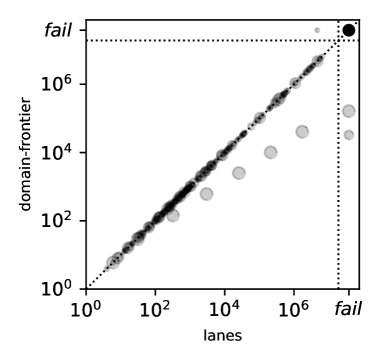
In order to empirically compare AND∗ using domain-frontier equivalence pruning with previous approaches, we re-run each previous approach adding the use of the concretizer. Table 3 shows the results. We verify that while the use of the concretizer allows the sound use of domain-frontier equivalence pruning, it has no empirical impact on the coverage of previous approaches. Domain-frontier equivalence pruning shows better results than identity and lanes equivalence pruning. Domain-frontier maintains the reduction of the number of generated policies lanes had over identity without meaningfully reducing it further, except in acrobatics, where the average number of generated policies is reduced from 837 to 197. Figure 6 depicts per task the differences in the number of generated policies between domain-frontier and lanes pruning. The main gain of domain-frontier pruning over lanes pruning is time reduction. Computing the domain-frontier signature is faster than computing , especially for large policies. This can be strongly perceived in beam-walk and doors domains, where the average execution time was reduced respectively from 65.71s to 0.22s and from 22.53s to 2.52s.
3.3 Frontier Equivalence Pruning
One can ask if the unsoundness problem we previously showed regarding the use of equivalence pruning still holds if we use the concretizer. This is a very reasonable question since domain-frontier equivalence pruning was not sound before and became sound with the use of the concretizer. Unfortunately, unsoundness is still the case for frontier equivalence pruning. In this subsection, we cope with the unsoundness of frontier equivalence pruning.
Figure 7 shows an example state space with five states: – the initial state –, , , , and – the single goal state. We use it to show the unsoundness of frontier equivalence pruning. The choices made by method (Algorithm 1) regarding which unmapped state to map when expanding a policy determine the specific policy space AND∗ is searching on. We analyze a possible policy space for this state space. The initial search node is and it has two successors: and . We note that and . Let’s say AND∗ chooses to map instead of for and instead of for . Then, the single successor of is and the single successor of is . We note that and . Both and are two steps away from becoming a solution policy. The critical problem is that both and will be pruned because and if AND∗ chooses to expand and before expanding either or . This kind of “crossed-mutual” pruning, where the descendent of some policy is pruned by the ancestor of another policy and vice-versa, cannot happen when using previous equivalence pruning concepts because implies/requires when is identity, lanes, or domain-frontier.101010We note that even if we prevent “crossed-mutual” prunings from occurring, there are more complex examples where frontier pruning is still unsound.
Despite unsound, AND∗ always terminates and never returns false-positive answers when using frontier equivalence pruning (Corollary 1, in Appendix A.1). With or without the concretizer, AND∗ always returns either or a solution. Never a non-solution policy . That’s the case because, by construction, it has no means of returning a policy that is not a solution, regardless of the choice of . We can use this fact to make AND∗ with frontier pruning sound and complete in a straightforward way. We make AND∗ first to run the search using frontier pruning, and then – only if the first search ends up returning – it re-runs the search from scratch using domain-frontier pruning. Optimality is lost here. We call that simply AND∗ with frontier pruning because the backup search was never required to be called in this work. Every time we ran AND∗ with frontier pruning, it always either failed by resource limits during the first search or found a solution through the first search.
| domain-frontier | frontier | |||||
| Domain | ||||||
| acrobatics | 1.00 | 0.00 | 0.00 | 1.00 | 0.00 | 0.00 |
| beam-walk | 0.82 | 0.18 | 0.00 | 0.82 | 0.18 | 0.00 |
| blocksworld-original | 0.50 | 0.33 | 0.17 | 0.53 | 0.47 | 0.00 |
| blocksworld-advanced | 0.20 | 0.64 | 0.16 | 0.20 | 0.71 | 0.09 |
| chain-of-rooms | 0.30 | 0.00 | 0.70 | 1.00 | 0.00 | 0.00 |
| earth-observation | 0.20 | 0.00 | 0.80 | 0.33 | 0.15 | 0.53 |
| elevators | 0.47 | 0.00 | 0.53 | 0.80 | 0.00 | 0.20 |
| faults | 0.40 | 0.00 | 0.60 | 0.56 | 0.00 | 0.44 |
| first-responders | 0.48 | 0.00 | 0.52 | 0.69 | 0.25 | 0.05 |
| tireworld-triangle | 1.00 | 0.00 | 0.00 | 1.00 | 0.00 | 0.00 |
| zenotravel | 0.33 | 0.67 | 0.00 | 0.33 | 0.67 | 0.00 |
| doors | 0.87 | 0.00 | 0.13 | 1.00 | 0.00 | 0.00 |
| islands | 0.42 | 0.00 | 0.58 | 0.63 | 0.00 | 0.37 |
| miner | 0.10 | 0.02 | 0.88 | 0.24 | 0.76 | 0.00 |
| tireworld-spiky | 0.45 | 0.00 | 0.55 | 0.82 | 0.18 | 0.00 |
| tireworld-truck | 0.18 | 0.00 | 0.82 | 0.46 | 0.00 | 0.54 |
| TOTAL | 0.48 | 0.11 | 0.40 | 0.65 | 0.21 | 0.14 |
| domain-frontier | frontier | ||||||
| Domain | |||||||
| acrobatics | 1.00 | 3.10 | 27,206 | 126.50 | 2.08 | 11,109 | 126.50 |
| beam-walk | 0.82 | 0.22 | 454 | 453.22 | 0.21 | 454 | 453.22 |
| blocksworld-original | 0.50 | 121.56 | 402,523 | 13.40 | 152.25 | 182,954 | 13.47 |
| blocksworld-advanced | 0.20 | 0.39 | 4,552 | 9.64 | 0.37 | 1,729 | 9.64 |
| chain-of-rooms | 0.30 | 1.83 | 118,996 | 57.00 | 0.40 | 828 | 57.00 |
| earth-observation | 0.20 | 7.30 | 693,463 | 13.88 | 0.08 | 3,725 | 14.00 |
| elevators | 0.47 | 0.39 | 42,196 | 14.86 | 0.07 | 383 | 14.86 |
| faults | 0.40 | 2.28 | 238,657 | 15.36 | 0.73 | 79,559 | 16.27 |
| first-responders | 0.48 | 4.96 | 487,417 | 8.03 | 8.47 | 18,001 | 8.08 |
| tireworld-triangle | 1.00 | 26.26 | 485 | 244.00 | 25.72 | 485 | 244.00 |
| zenotravel | 0.33 | 2.33 | 1,808 | 14.80 | 2.33 | 934 | 14.80 |
| doors | 0.87 | 9.05 | 5,048 | 5,038.62 | 7.86 | 5,048 | 5,038.62 |
| islands | 0.42 | 2.96 | 575,809 | 4.84 | 0.67 | 17,057 | 4.84 |
| miner | 0.10 | 212.47 | 2,209,231 | 14.20 | 214.63 | 166,141 | 14.20 |
| tireworld-spiky | 0.45 | 49.41 | 1,268,072 | 25.00 | 37.97 | 138,650 | 25.00 |
| tireworld-truck | 0.18 | 3.20 | 511,915 | 13.15 | 0.15 | 2,568 | 13.15 |
| TOTAL | 0.48 | 4.89 | 60,651 | 34.70 | 2.11 | 6,305 | 34.87 |
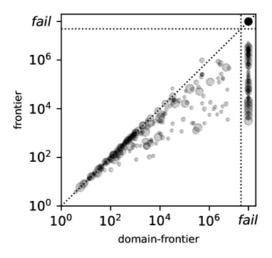
We empirically compare AND∗ using frontier and domain-frontier equivalence pruning (Table 4). We can check that there was an expressive increase in coverage in comparison to domain-frontier equivalence pruning (from 0.48 to 0.65). Major gains have occurred in chain-of-rooms (from 0.30 to 1.00), elevators (from 0.47 to 0.80), first-responders (from 0.48 to 0.69), islands (from 0.42 to 0.63), tireworld-spiky (from 0.45 to 0.82), and tireworld-truck (from 0.18 to 0.46). There is a dramatic improvement in the number of generated policies in most domains. Decreases of at least 50% have occurred in acrobatics, blocksworld-original, blocksworld-advanced, chain-of-rooms, earth-observation, elevators, faults, first-responders, zenotravel, islands, miner, tireworld-spiky, and tireworld-truck – all but three domains. Decreases of at least one order of magnitude have occurred in seven domains: chain-of-rooms, earth-observation, elevators, first-responders, islands, miner, and tireworld-truck. Figure 8 depicts per task the differences in the number of generated policies between frontier and domain-frontier pruning.
4 Improving Equivalence Pruning with State Symmetries
In this section, we focus on strengthening the pruning effect of policy frontier equivalence through state symmetries. We study symmetries that capture the concept that “symmetrical” states generate “symmetrical” trajectories in the state space. Let be a function with that maps symmetrical states to the same signature. Each signature defines an equivalence class of states. Using this function, we can define a new frontier signature function for AND∗ policies as . With this function, policies are considered equivalent iff they contain in their the same number of states from each equivalence class of symmetrical states.
Structural state symmetries (Pochter et al., 2011; Shleyfman et al., 2015) capture part of all existing state symmetries, and Winterer et al. (2016) shows we can apply the concept of structural state symmetries for FOND planning. We evaluate the empirical impact of using two techniques to find structural state symmetries: an approximated (greedy) approach and the perfect approach. Pochter et al. (2011) and Winterer et al. (2016) compute structural state symmetries using a greedy hill-climbing procedure given that the problem was considered intractable in practice. We show that we can in practice efficiently compute them perfectly using group theory techniques from Jefferson et al. (2019)’s work.
4.1 Structural State Symmetries
Let be a FOND task. A structural symmetry for is111111We combine the definitions from Shleyfman et al. (2015) and Winterer et al. (2016) works. The former defines structural symmetries for classical planning tasks in STRIPS (Fikes and Nilsson, 1971), while the latter defines them for FOND planning tasks in SAS+ (Bäckström and Nebel, 1995). Since our work’s running definition of FOND tasks uses the STRIPS formalism, our formal definition of structural symmetries is an adaptation of theirs. We use SAS+ in our implementation, and we talk about it later here. a permutation , such that:
-
1.
, where is a permutation of facts and is a permutation of actions;
-
2.
; and
-
3.
and , for each .
We overload , so that, for each state , denotes the state with . We note that if is structural symmetry, is a goal state if and only if is a goal state. Moreover, an action is applicable to if and only if the action is applicable to . Finally, the set is equal to the set .
The definition of structural symmetries we use actually has two extra conditions:
-
4.
, for each , where is a given partition of the facts; and
-
5.
, for each , where is a given partition of the actions.
The partition comes from the fact we use a SAS+ (Bäckström and Nebel, 1995) formalism to represent the FOND tasks in our implementation. When using SAS+, facts are partitioned into variables such that, for each variable, exactly one fact of that variable is true at each state. This allows a more compact representation of actions and states (Helmert, 2009). With the first extra restriction, our definition of structural symmetries matches the definition from Winterer et al. (2016).
The second extra restriction is an optimization. We look only for structural symmetries that permute actions that were grounded from the same lifted action. This loses possible symmetries between distinct lifted actions but allows a more focused computation of structural symmetries.
The objective is to have a canonical function such that iff exists a structural symmetry with . Of course, if is a structural symmetry, then also is. Let be the permutation group containing all structural symmetries for . We denote for each , and we note that for each . Therefore, if we have a relation of total order over states, and we let (with ) to return the minimal state in w.r.t. , then we can set . This function is canonical. The problem is that can be too large even to be enumerated. In the worst case, the size of is factorial to the size of facts and actions.
Pochter et al. (2011) and Shleyfman et al. (2015) show we can compute a generator for using the Problem Description Graph (PDG) of the task. A generator of a permutation group is a set of permutations , such that for every permutation , exists some sequence of permutations in , possibly with repetitions, such that the result of their combination, in order, is . In other words, a generator of a permutation group is a compact representation of .
Winterer et al. (2016) approximate the desired function using a greedy hill-climbing procedure on the local state neighbourhood provided by the direct application of generator permutations – i.e. where is the computed generator of . They define to be the result of the hill-climbing procedure starting from . If for the defined from this greedy hill-climbing procedure, then also for a canonical , but the opposite is not always true.
In this work, we apply a technique presented by Jefferson et al. (2019) that allows the computation of the canonical signature of a state by using the stabilizer chain of . Their work is a work on group theory, and deals with permutation groups in general. We show that with their technique121212Throughout their work, they present more than one technique to compute the canonical image of a subset of elements w.r.t. to a permutation group that acts on those elements. We actually use a simplified version of their simplest presented technique (FixedOrbit). The impact of using the other presented techniques is an interesting question for future work., we are able to compute a canonical signature of states almost as fast as we can compute a greedy signature using the hill-climbing procedure. As far as we know, this is the first time their work is being applied to planning.
4.2 Empirical Evaluation
| Domain | sym. tasks | |
|---|---|---|
| IPC-FOND | acrobatics | none |
| beam-walk | none | |
| chain-of-rooms | none | |
| tireworld-triangle | none | |
| earth-observation | just one | |
| blocksworld-original | ||
| blocksworld-advanced | ||
| elevators | ||
| faults | all but one | |
| first-responders | all but one | |
| zenotravel | all | |
| NEW-FOND | doors | none |
| tireworld-truck | ||
| tireworld-spiky | all but one | |
| islands | all but one | |
| miner | all |
Table 5 shows, for each domain, the ratio of tasks with structural symmetries (besides the identity symmetry). For eight of the 16 domains, at least 80% of tasks in each domain present structural symmetries. And for ten, at least half the tasks present structural symmetries. We use Nauty (McKay and Piperno, 2014) to compute automorphism group generators of PDGs, from which we can extract generators. We are able to compute a generator of in at most 1.75 seconds for all tasks that have symmetries. We set an overcautious time limit of five seconds for this computation. If Nauty fails to conclude its execution within this time limit, the use of structural symmetries is disabled. It only fails for tasks p7 and p8 of acrobatics, tasks p6 to p11 of beam-walk, and tasks p11 to p40 of tireworld-triangle – all of which likely do not have structural symmetries because, in these domains, the computation does not find symmetries for all tasks where it concludes. We use GAP (Groups, Algorithms, and Programming software) to compute stabilizer chains of permutation groups. For every task where computing within time limits was successful, we are able to compute the stabilizer chain of in at most five extra seconds.
| none | greedy | canonical | |||||||
| Domain | |||||||||
| acrobatics | 1.00 | 0.00 | 0.00 | 1.00 | 0.00 | 0.00 | 1.00 | 0.00 | 0.00 |
| beam-walk | 0.82 | 0.18 | 0.00 | 0.82 | 0.18 | 0.00 | 0.82 | 0.18 | 0.00 |
| blocksworld-original | 0.53 | 0.47 | 0.00 | 0.53 | 0.47 | 0.00 | 0.53 | 0.47 | 0.00 |
| blocksworld-advanced | 0.20 | 0.71 | 0.09 | 0.20 | 0.71 | 0.09 | 0.20 | 0.71 | 0.09 |
| chain-of-rooms | 1.00 | 0.00 | 0.00 | 1.00 | 0.00 | 0.00 | 1.00 | 0.00 | 0.00 |
| earth-observation | 0.33 | 0.15 | 0.53 | 0.33 | 0.15 | 0.53 | 0.33 | 0.15 | 0.53 |
| elevators | 0.80 | 0.00 | 0.20 | 0.80 | 0.00 | 0.20 | 0.80 | 0.00 | 0.20 |
| faults | 0.56 | 0.00 | 0.44 | 1.00 | 0.00 | 0.00 | 1.00 | 0.00 | 0.00 |
| first-responders | 0.69 | 0.25 | 0.05 | 0.73 | 0.25 | 0.01 | 0.75 | 0.24 | 0.01 |
| tireworld-triangle | 1.00 | 0.00 | 0.00 | 1.00 | 0.00 | 0.00 | 1.00 | 0.00 | 0.00 |
| zenotravel | 0.33 | 0.67 | 0.00 | 0.33 | 0.67 | 0.00 | 0.33 | 0.67 | 0.00 |
| doors | 1.00 | 0.00 | 0.00 | 1.00 | 0.00 | 0.00 | 1.00 | 0.00 | 0.00 |
| islands | 0.63 | 0.00 | 0.37 | 0.80 | 0.13 | 0.07 | 0.80 | 0.13 | 0.07 |
| miner | 0.24 | 0.76 | 0.00 | 0.55 | 0.45 | 0.00 | 0.53 | 0.47 | 0.00 |
| tireworld-spiky | 0.82 | 0.18 | 0.00 | 1.00 | 0.00 | 0.00 | 1.00 | 0.00 | 0.00 |
| tireworld-truck | 0.46 | 0.00 | 0.54 | 0.57 | 0.00 | 0.43 | 0.57 | 0.00 | 0.43 |
| TOTAL | 0.65 | 0.21 | 0.14 | 0.73 | 0.19 | 0.08 | 0.73 | 0.19 | 0.08 |
none greedy canonical Domain acrobatics 1.00 2.08 11,109 126.50 3.36 11,109 126.50 3.36 11,109 126.50 beam-walk 0.82 0.21 454 453.22 2.45 454 453.22 2.45 454 453.22 blocksworld-original 0.53 229.56 270,882 14.12 229.84 270,709 14.12 229.86 270,708 14.12 blocksworld-advanced 0.20 0.37 1,729 9.64 0.37 1,730 9.64 0.49 1,730 9.64 chain-of-rooms 1.00 33.01 7,968 162.00 33.75 7,968 162.00 33.29 7,968 162.00 earth-observation 0.32 2.72 219,401 26.08 2.83 219,178 26.08 2.74 219,172 26.08 elevators 0.80 8.87 374,049 25.33 5.49 161,881 25.33 6.56 161,881 25.33 faults 0.56 4.80 534,692 19.13 0.06 273 19.13 0.73 273 19.13 first-responders 0.69 84.72 244,376 10.63 59.93 172,288 10.71 60.78 171,978 10.71 tireworld-triangle 1.00 25.72 485 244.00 29.46 485 244.00 30.31 485 244.00 zenotravel 0.33 2.33 934 14.80 1.93 689 14.80 2.72 689 14.80 doors 1.00 118.06 17,484 17,473.73 114.54 17,484 17,473.73 117.27 17,484 17,473.73 islands 0.63 22.38 373,141 5.74 3.23 21,403 5.74 8.66 19,214 5.74 miner 0.24 623.20 978,423 15.33 138.27 153,427 15.33 147.98 153,427 15.33 tireworld-spiky 0.82 380.18 918,175 25.00 1.70 3,798 25.00 2.41 3,798 25.00 tireworld-truck 0.46 27.17 488,319 13.94 0.27 4,454 13.94 0.80 4,454 13.94 TOTAL 0.65 15.60 44,784 45.43 5.81 10,012 45.45 8.38 9,944 45.45
We compare using greedy and canonical structural symmetries against not using state symmetries (Table 6). The results demonstrate that Jefferson et al. (2019)’s contributions allow a fast computation of canonical structural symmetries. Computing the canonical structural symmetries takes only more (aggregated) time per generated policy than computing the structural symmetries through hill-climbing for the solved tasks. On the other hand, the greedy structural symmetries provided by the hill-climbing procedure prove effective, as only more policy generations are required to solve the solved tasks on average, a difference that comes almost exclusively from the domain of islands.
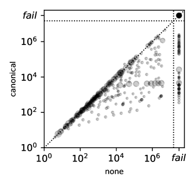
Both approaches improve AND∗’s performance towards a coverage of , much superior to the coverage of we had before using state symmetries. The number of generated policies reduces by at least when using state symmetries on the domains of elevators, faults, zenotravel, islands, miner, tireworld-spiky, and tireworld-truck. The reduction is dramatic in faults (), tireworld-spiky (), and tireworld-truck (). Figure 9 depicts per task the differences in the number of generated policies between using canonical symmetries and not using structural symmetries. The gains in coverage occur in faults, first-responders, islands, miner, tireworld-spiky, and tireworld-truck. The major gains are in faults (from to ) and miner (from to and ). No change occurs in domains without structural symmetries besides the increase in execution time due to the execution of Nauty. The returned solution size remains, in general, mostly unchanged. We decide to stick with canonical structural state symmetries for the remainder of this work.
5 Search Improvements
In this section, we evaluate satisficing search techniques to increase the capacity of the planner to find solutions for FOND tasks.
5.1 Deadlock Detection
| without dld | with dld | |||||
| Domain | ||||||
| acrobatics | 1.00 | 0.00 | 0.00 | 1.00 | 0.00 | 0.00 |
| beam-walk | 0.82 | 0.18 | 0.00 | 0.82 | 0.18 | 0.00 |
| blocksworld-original | 0.53 | 0.47 | 0.00 | 0.57 | 0.43 | 0.00 |
| blocksworld-advanced | 0.20 | 0.71 | 0.09 | 0.20 | 0.71 | 0.09 |
| chain-of-rooms | 1.00 | 0.00 | 0.00 | 1.00 | 0.00 | 0.00 |
| earth-observation | 0.33 | 0.15 | 0.53 | 0.33 | 0.15 | 0.53 |
| elevators | 0.80 | 0.00 | 0.20 | 0.80 | 0.00 | 0.20 |
| faults | 1.00 | 0.00 | 0.00 | 1.00 | 0.00 | 0.00 |
| first-responders | 0.75 | 0.24 | 0.01 | 0.76 | 0.24 | 0.00 |
| tireworld-triangle | 1.00 | 0.00 | 0.00 | 1.00 | 0.00 | 0.00 |
| zenotravel | 0.33 | 0.67 | 0.00 | 0.33 | 0.67 | 0.00 |
| doors | 1.00 | 0.00 | 0.00 | 1.00 | 0.00 | 0.00 |
| islands | 0.80 | 0.13 | 0.07 | 0.80 | 0.13 | 0.07 |
| miner | 0.53 | 0.47 | 0.00 | 0.55 | 0.45 | 0.00 |
| tireworld-spiky | 1.00 | 0.00 | 0.00 | 1.00 | 0.00 | 0.00 |
| tireworld-truck | 0.57 | 0.00 | 0.43 | 0.97 | 0.00 | 0.03 |
| TOTAL | 0.73 | 0.19 | 0.08 | 0.76 | 0.19 | 0.06 |
| without dld | with dld | ||||||
| Domain | |||||||
| acrobatics | 1.00 | 3.36 | 11,109 | 126.50 | 3.30 | 11,109 | 126.50 |
| beam-walk | 0.82 | 2.45 | 454 | 453.22 | 87.16 | 454 | 453.22 |
| blocksworld-original | 0.53 | 229.86 | 270,708 | 14.12 | 213.44 | 256,179 | 14.12 |
| blocksworld-advanced | 0.20 | 0.49 | 1,730 | 9.64 | 0.49 | 1,671 | 9.64 |
| chain-of-rooms | 1.00 | 33.29 | 7,968 | 162.00 | 23.61 | 5,467 | 162.00 |
| earth-observation | 0.32 | 2.74 | 219,172 | 26.08 | 2.75 | 219,172 | 26.08 |
| elevators | 0.80 | 6.56 | 161,881 | 25.33 | 3.57 | 43,606 | 24.92 |
| faults | 1.00 | 0.87 | 1,050 | 24.31 | 0.90 | 1,050 | 24.31 |
| first-responders | 0.75 | 127.49 | 297,969 | 11.66 | 128.60 | 297,825 | 11.62 |
| tireworld-triangle | 1.00 | 30.31 | 485 | 244.00 | 30.41 | 485 | 244.00 |
| zenotravel | 0.33 | 2.72 | 689 | 14.80 | 2.73 | 689 | 14.80 |
| doors | 1.00 | 117.27 | 17,484 | 17,473.73 | 118.26 | 17,484 | 17,473.73 |
| islands | 0.80 | 75.48 | 207,497 | 6.21 | 76.02 | 207,497 | 6.21 |
| miner | 0.53 | 502.24 | 416,280 | 16.33 | 506.11 | 416,280 | 16.33 |
| tireworld-spiky | 1.00 | 4.75 | 5,913 | 25.73 | 4.36 | 4,922 | 25.73 |
| tireworld-truck | 0.57 | 1.25 | 5,618 | 14.64 | 1.26 | 3,644 | 14.55 |
| TOTAL | 0.73 | 11.75 | 14,423 | 47.02 | 13.77 | 12,417 | 46.94 |
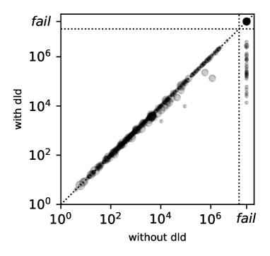
Messa and Pereira (2023) present a relatively efficient way of incrementally determining whether a candidate policy has deadlocks (i.e. is unproper) based on the assumption that its predecessor had none. This kind of procedure is called deadlock detection and effectively allows the early discard of some of the policies that certainly won’t become a solution (since no solution has deadlocks). However, when using the concretizer, deadlocks can be fixed as long the policy we have has correct and sets, as we saw in Subsection 3.2. Therefore, when using the concretizer, policies with deadlocks might actually lead to a solution. Nevertheless, using deadlock detection is still a possibility, and it can be useful to focus the exploration on directions that do not involve dealing with deadlocks.
We verify the empirical impact of enabling deadlock detection on AND∗ with frontier pruning and structural symmetries. We discard policies with deadlocks upon generation. This way, the signatures of discarded policies are not included in . Table 7 shows the results. We verify that while its computation is slow for beam-walk large policies, it has a dramatic positive impact on the domain of tireworld-truck. The coverage of tireworld-truck increases from 0.57 to 0.97, causing the aggregated coverage to increase from 0.73 to 0.76. Other domains remain fairly stable. Figure 10 depicts per task the differences in the number of generated policies. We decide to stick with deadlock detection for the remainder of this work.
AND∗ with deadlock detection is only sound when using identity and lanes equivalence pruning. With domain-frontier or frontier equivalence pruning, AND∗ may return false negatives when using deadlock detection. In our experiments, AND∗ never returns false negatives. It always finds a solution or fails due to resource limits.
5.2 Sub-Obtimal Search
In classical planning, a baseline satisficing technique is to perform a sub-optimal search, and a straightforward way of performing a sub-optimal search by changing the guiding heuristic function from to , for some . The modified version of A∗ that applies this modification is called Weighted A∗ (WA∗) (Pohl, 1970). When using an admissible, goal-aware and consistent heuristic, WA∗ is ensured to return a solution within the factor from the optimality. A more extreme variant, called Greedy Best-First Search (GBFS) (Doran and Michie, 1966), expands first nodes with least , regardless of their -value, which is then used solely for tie-breaking (greater first). GBFS is the expected version of Weighted A∗ when (except for the expected tie-breaker, which is reversed), and it is a core classical heuristic search engine when solution optimality is not important (Russell and Norvig, 2016).
Since we already have waived optimality, and our current goal is to increase the AND∗’s capacity to find solutions for FOND tasks, it is reasonable to empirically evaluate the performance of AND∗ using such modified heuristic functions. Since the FOND heuristic we are using, , directly returns -values instead of -values, we derive as . Then, we recompute the -values using the above-mentioned formulas. We call AND∗ -Weighted A∗ with Non-Determinism (-WAND∗) and when expanding first nodes with least and Greedy Best-First Search with Non-Determinism (GBFSND) when expanding first nodes with least .
| AND∗ | 2-WAND∗ | GBFSND | |||||||
| Domain | |||||||||
| acrobatics | 1.00 | 0.00 | 0.00 | 1.00 | 0.00 | 0.00 | 1.00 | 0.00 | 0.00 |
| beam-walk | 0.82 | 0.18 | 0.00 | 0.82 | 0.18 | 0.00 | 0.82 | 0.18 | 0.00 |
| blocksworld-original | 0.57 | 0.43 | 0.00 | 0.93 | 0.07 | 0.00 | 0.40 | 0.60 | 0.00 |
| blocksworld-advanced | 0.20 | 0.71 | 0.09 | 0.67 | 0.33 | 0.00 | 0.18 | 0.82 | 0.00 |
| chain-of-rooms | 1.00 | 0.00 | 0.00 | 1.00 | 0.00 | 0.00 | 1.00 | 0.00 | 0.00 |
| earth-observation | 0.33 | 0.15 | 0.53 | 0.45 | 0.12 | 0.42 | 1.00 | 0.00 | 0.00 |
| elevators | 0.80 | 0.00 | 0.20 | 0.93 | 0.00 | 0.07 | 1.00 | 0.00 | 0.00 |
| faults | 1.00 | 0.00 | 0.00 | 1.00 | 0.00 | 0.00 | 1.00 | 0.00 | 0.00 |
| first-responders | 0.76 | 0.24 | 0.00 | 0.97 | 0.03 | 0.00 | 0.65 | 0.35 | 0.00 |
| tireworld-triangle | 1.00 | 0.00 | 0.00 | 1.00 | 0.00 | 0.00 | 1.00 | 0.00 | 0.00 |
| zenotravel | 0.33 | 0.67 | 0.00 | 0.53 | 0.47 | 0.00 | 0.60 | 0.40 | 0.00 |
| doors | 1.00 | 0.00 | 0.00 | 1.00 | 0.00 | 0.00 | 1.00 | 0.00 | 0.00 |
| islands | 0.80 | 0.13 | 0.07 | 0.75 | 0.17 | 0.08 | 0.52 | 0.48 | 0.00 |
| miner | 0.55 | 0.45 | 0.00 | 0.47 | 0.53 | 0.00 | 0.04 | 0.96 | 0.00 |
| tireworld-spiky | 1.00 | 0.00 | 0.00 | 1.00 | 0.00 | 0.00 | 0.27 | 0.73 | 0.00 |
| tireworld-truck | 0.97 | 0.00 | 0.03 | 1.00 | 0.00 | 0.00 | 0.54 | 0.38 | 0.08 |
| TOTAL | 0.76 | 0.19 | 0.06 | 0.85 | 0.12 | 0.04 | 0.69 | 0.31 | 0.01 |
AND∗ 2-WAND∗ GBFSND Domain acrobatics 1.00 3.30 11,109 126.50 3.33 10,926 126.50 3.17 315 126.50 beam-walk 0.82 87.16 454 453.22 86.20 454 453.22 85.58 454 453.22 blocksworld-original 0.40 69.16 69,337 11.75 0.99 243 12.25 1.40 914 182.58 blocksworld-advanced 0.18 0.38 1,333 9.20 0.23 80 9.40 0.24 75 11.80 chain-of-rooms 1.00 23.61 5,467 162.00 3.32 376 162.00 3.31 376 162.00 earth-observation 0.32 2.75 219,172 26.08 1.70 114,713 26.38 0.11 119 33.85 elevators 0.80 3.57 43,606 24.92 0.69 1,625 25.83 0.67 715 117.42 faults 1.00 0.90 1,050 24.31 0.82 123 23.00 0.83 121 23.00 first-responders 0.61 75.11 324,363 11.50 1.15 3,485 12.83 40.25 32,307 841.67 tireworld-triangle 1.00 30.41 485 244.00 27.86 485 244.00 30.28 485 244.00 zenotravel 0.33 2.73 689 14.80 1.73 325 16.00 2.32 583 31.60 doors 1.00 118.26 17,484 17,473.73 118.11 17,484 17,473.73 117.48 17,484 17,473.73 islands 0.52 1.42 6,061 5.52 2.38 11,734 5.52 75.60 27,567 1,421.68 miner 0.04 2.98 12,542 15.50 2.66 11,104 15.50 65.22 89,887 4,628.00 tireworld-spiky 0.27 0.98 2,289 25.00 1.08 2,877 25.00 24.20 33,523 4,472.67 tireworld-truck 0.54 1.29 41,165 15.60 0.91 6,868 15.60 88.55 512,812 1,102.17 TOTAL 0.62 6.31 8,106 45.87 2.71 1,861 46.57 7.28 2,178 308.49
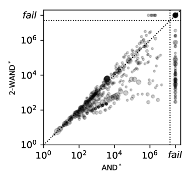
Table 8 shows the results of 2-WAND∗ and GBFSND against AND∗. We verify a drop in coverage when using GBFSND (from 0.76 to 0.69) but an increase in coverage when using 2-WAND∗ (from 0.76 to 0.85). The major gains of 2-WAND∗ occur in blockworld-original (from 0.57 to 0.93), blocksworld-advanced (from 0.20 to 0.67), first-responders (from 0.76 to 0.97), and zenotravel (from 0.33 to 0.53). GBFSND loses coverage in several domains but interestingly dramatically increases the coverage of earth-observation from 0.33 to 1.00. Increases in coverage have occurred in conjunction with big decreases in the number of generated policies. The decrease is dramatic in some cases. For instance, 2-WAND∗ reduced the average number of generated policies from 69,337 to 243 in blocksworld-original in the intersection of solved tasks. Figure 3 depicts per task the differences in the number of generated policies between 2-WAND∗ and AND∗. While the average size of returned policies dramatically increases using GBFSND, this metric remains mostly stable when using 2-WAND∗ in comparison to AND∗. In fact, 2-WAND∗ even returns slightly smaller solutions than AND∗ for faults. We decide to stick with 2-WAND∗ for the remainder of this work. Since 2-WAND∗ is just AND∗ running with another heuristic function, it is included when we generally-talk about AND∗ later in discussions.
6 Solution Compressing
In this section, we introduce a procedure, called the compressor, that allows the compression of solution policies. The compressor receives as input a policy defined over states, and returns a policy defined over partial states that is optimal (has the minimum number of partial states), such that maps each state in the to the same action it is mapped in , and maps no state in the . The central idea of the compressor is to use an integer program iteratively, which is fast in practice, to determine the partial states part of policy . The compressor is a general procedure and can compress solutions of any planner that finds policies defined over states.
6.1 Partial States and Partial Policies
A partial state is a partial function . Partial states represent simple properties regarding the truth valuation of facts, allowing the concise representation of the set of states with such a property. We note that we can view a state as a total function with iff . We say a state holds a property (partial state) – denoted – iff, for each , is undefined or . The set of states represented by a partial state is . We can perceive the task goal condition and the action preconditions as partial states. A partial policy is a partial function mapping partial states to actions. For a given state , we define . Note that is a set of actions. We define . is a partial function mapping states to actions, and it maps a state iff is a singleton. Therefore, there are two distinct ways for a state to become unmapped on . Namely, if either or . We use to contain each state that becomes unmapped on because there are multiple partial states in representing it, and they don’t agree on the action. Let . A partial policy is a solution partial policy for iff is a solution policy for and .131313We ensure no state with is reachable because there are multiple ways to deal with such states. Setting is just one possibility. Therefore, if we were to let , one would need to be informed about how to proceed at states in order to use properly. Some works set an external rule that defines which action should be used at if . For instance, by presenting a total order for the mappings in .
6.2 The Compressor
Algorithm 6 displays the pseudocode for the compressor. The compressor allows the compression of any given into a partial policy such that and , with minimal . In other words, it produces a partial policy such that agrees with for each and does not map any state . Additionally, it ensures for each state .
In order for to agree with in the mapping of some state , must be . Therefore, there must exist at least one partial state with mapped to in (otherwise ), and there must exist no other partial state with mapped to other action besides in (otherwise ). That is enough to ensure an agreement of and regarding states in . We additionally enforce that no partial state in represents any state in .
The compressor subdivides the original problem of deciding all the mappings of into subproblems of deciding all the mappings to each action. For each action, it finds the minimal set of partial states that covers all states that need to be mapped to that action without covering any other domain or frontier state from . The resulting partial policy has since agrees with for all states in and has for all states in . Since we ensure for each , we have . Therefore, the resulting partial policy is a solution partial policy when the input policy is a solution policy.
6.3 Finding the Minimal-Sized Set of Partial States
Differently from the concretizer presented previously, the compressor does not run in polynomial time. To find the minimal set of partial states that fulfils the required conditions, we repeatedly try to solve an integer programming problem with an increasing number of partial states, starting from one.
The following integer program models the task of determining whether there is or not a set of partial states representing each but no .
For each partial state , with , we have a boolean variable for each and ,141414Since our implementation uses SAS+ FOND tasks instead of STRIPS FOND tasks the actual IPs we produce has variables , where is a variable and . Despite we present the IPs for STRIPS FOND tasks, every aspect described here can be directly translated to an analogous aspect we would have in IPs for SAS+ FOND tasks. and a boolean variable for each . means and means .
The first set of constraints ensures each is represented by some partial state . The second set of constraints ensures each is not represented by any partial state . The third and fourth sets of constraints ensure the semantics of . The third enforces not to map any fact differently than if . While the fourth enforces to map some fact differently than if . The fifth set of constraints ensures maps each fact to at most one truth valuation.
Since we try to solve the problem first with , then with , and so on, until it is solvable (and certainly it will be if reaches ), we don’t need to model the optimization of in the integer program. The optimization function minimizes instead the total number of facts mapped through the fixed partial states. While we could instead minimize zero, in order to have an easier integer program, this provides a much more human-readable output and also provides heuristic guidance for the integer programming solver we use.
We now simplify this integer program. Firstly, we note that since every must be zero if , then we can fully remove the second set of constraints by replacing these variables with a constant zero in every other constraint they appear. This makes the third set of constraints trivial for , so we make the third set of constraints exist only for .
Secondly, we note that the fourth set of constraints is irrelevant for . They hinder from occurring simultaneously with for some and some . However, allowing that causes no problem. Whenever that situation is possible, considering the other constraints, changing to is also possible. Thus no extra solution is ever permitted by removing the constraints for in the fourth set of constraints. Moreover, we don’t use the values of variables when extracting the set of partial states , so they do not need to be precise. Therefore, we make the fourth set of constraints exist only for .
Thirdly, the fifth set of constraints is irrelevant because it can only hurt to set both and for some fact , since this makes useless as it will not be able to represent any state in . And since we only try solving with partial states after failing to solve with (or if ), no solution has some useless . So we remove these constraints.
The integer program resulting from these simplifications is shown below.
Additionally, we note that we just need to create a variable only if there is at least one state with . Otherwise, this variable is useless, as it will always be zero in some solution.
The approach of first subdividing the original compression problem into a subproblem for each action and then trying to solve it with an increasing number of partial states using this optimized IP formulation was critical to have a sufficiently fast and memory-efficient procedure to compress the solutions returned by 2-WAND∗.
6.4 Empirical Evaluation
| Domain | |||
|---|---|---|---|
| acrobatics | 1.00 | 126.50 | 126.50 |
| beam-walk | 0.82 | 453.22 | 453.22 |
| blocksworld-original | 0.93 | 23.21 | 22.86 |
| blocksworld-advanced | 0.67 | 32.00 | 27.62 |
| chain-of-rooms | 1.00 | 162.00 | 162.00 |
| earth-observation | 0.45 | 33.67 | 27.56 |
| elevators | 0.93 | 30.79 | 28.00 |
| faults | 1.00 | 23.00 | 14.18 |
| first-responders | 0.97 | 16.10 | 14.78 |
| tireworld-triangle | 1.00 | 244.00 | 163.00 |
| zenotravel | 0.53 | 25.50 | 25.25 |
| doors | 1.00 | 17,473.73 | 18.00 |
| islands | 0.75 | 6.11 | 6.11 |
| miner | 0.47 | 16.33 | 16.33 |
| tireworld-spiky | 1.00 | 25.73 | 22.36 |
| tireworld-truck | 1.00 | 18.64 | 14.69 |
| TOTAL | 0.85 | 57.37 | 33.32 |
We tried to compress the solutions returned by 2-WAND∗ using the compressor. We use IBM’s ILOG CPLEX to solve integer programming problems. For each solved task, the compressor was able to compress the returned solution within the memory and time limits that remained after the execution performed by 2-WAND∗. For the majority of the tasks, we are able to compress the solutions returned in less than 40ms. Besides p15, p14, and p13 of doors, all other solved tasks had their returned solutions compressed in at most six seconds. The most time-consuming compression (on p15 of doors) took 91 seconds to complete. Only four domains have some task for which the returned solution took more than one second to be compressed: beam-walk, chain-of-rooms, doors, and tireworld-triangle. The domain of doors is especially hard because, while the largest solution returned for some other domain has size 2,047 (from p9 of beam-walk), the optimal solution size of p15 of doors is 131,070 before compression.
Table 9 shows that the compressor reduces the size of the returned solution in 12 of the 16 domains. Decreases of at least 10 occur in seven: blockworld-advanced, earth-observation, faults, tireworld-triangle, doors, tire-world-spiky, and tireworld-truck. In doors, the decrease is dramatic. The average size of returned solutions decreases three orders of magnitude in doors.
In the next section, we compare the after-compression size of 2-WAND∗ returned solutions with the size of solutions returned by two state-of-the-art FOND planners that natively reason over partial states.
7 Comparison with the State of the Art
We preamble this section with a quick summary of previous results. Table 10 summarizes the main empirical results up to this point and we verify a gradual increase in coverage through the presented versions of AND∗. In particular, we note that the key increases have occurred in three moments: when we introduced frontier equivalence pruning, when we incorporated structural symmetries, and when we modified the evaluation function waiving its admissible nature. After all the changes, the ratio of unsolved tasks was reduced by times, from 0.55 to 0.15, and the average number of generated policies was reduced by two orders of magnitude on the intersection of tasks solved by all versions. The average size of the returned solution remained mostly stable until the introduction of the compressor, when it had a substantial drop, as we have just seen in the previous section.
| Version of AND∗ | ||||
|---|---|---|---|---|
| AND∗ | 0.45 | 57,958 | 28.69 | |
| AND∗ + lanes E.P. | 0.47 | 33,216 | 28.69 | |
| AND∗ + domain-frontier E.P. | 0.48 | 30,314 | 28.69 | |
| AND∗ + frontier E.P. | 0.65 | 3,834 | 28.84 | |
| AND∗ + s.s. frontier E.P. | 0.73 | 1,432 | 28.86 | |
| AND∗ + s.s. frontier E.P. + dld | 0.76 | 1,371 | 28.84 | |
| 2-WAND∗ + s.s. frontier E.P. + dld | 0.85 | 514 | 29.25 | |
| 2-WAND∗ + s.s. frontier E.P. + dld + comp. | 0.85 | 514 | 19.22 |
In this section, we compare the best version of AND∗ (2-WAND∗ with frontier pruning, structural symmetries, deadlock detection, and solution compression) with some FOND planners from the literature. We choose to compare AND∗ with PRP (Muise et al., 2012), FOND-SAT (Geffner and Geffner, 2018), and IDFSP (Pereira et al., 2022).
7.1 Comparison with the State of the Art
PRP (Muise et al., 2012) is a long-standing state-of-the-art satisficing FOND planner. PRP uses a classical planner to find trajectories to the goal. Starting by finding a trajectory from the initial state to the goal, it constructs a partial policy by repeatedly generalizing each new trajectory found using partial states. This process repeats until all the states reachable by the decompressed version of the current partial policy are covered, or until it concludes that one of them is a dead-end. In the case of the latter, it learns a constraint that prevents the same error from occurring again after it restarts the search.
FOND-SAT (Geffner and Geffner, 2018) compiles FOND tasks into SAT instances. When trying to solve a FOND task, it constructs a series of SAT instances that encode requirements a partial policy (with an increasing number of partial states) would need to have in order to be a solution for the given task, until one of them is solved. From the solution of the solved SAT instance, it extracts a compact solution partial policy for the FOND task. FOND-SAT aims to have good scalability in tasks with high degrees of non-determinism due to the fact that different branching futures can be dealt with in conjunction with the SAT formulation.
IDFSP (Pereira et al., 2022) is a state-of-the-art satisficing FOND planner. IDFSP solves FOND tasks by performing an iterative depth-first implicit policy-space search. Bounded by an increasing search depth limit, it first tries to find a trajectory from the initial state to the goal. By doing so, it implicitly maps each state in the sequence to an action. Then, in a depth-first manner, it tries to find a goal trajectory for each other state reachable by this implicit policy. In case of a dead-end or failure, it backtracks, removing mappings from the implicit policy. It uses different rules to cut short the exploration in some directions, taking into account the current search depth limit, the heuristic value of the states, and the previous explorations of those states. In case of ultimate failure, it restarts the search with an increased search depth limit.
We run each of them in their recommended settings and compare them with the best version of AND∗.
| IDFSP | PRP | FOND-SAT | 2-WAND∗ | ||||||||
| Domain | |||||||||||
| acrobatics | 1.00 | 0.00 | 0.00 | 1.00 | 0.00 | 0.00 | 0.38 | 0.62 | 1.00 | 0.00 | 0.00 |
| beam-walk | 1.00 | 0.00 | 0.00 | 1.00 | 0.00 | 0.00 | 0.18 | 0.82 | 0.82 | 0.18 | 0.00 |
| blocksworld-original | 0.97 | 0.03 | 0.00 | 1.00 | 0.00 | 0.00 | 0.33 | 0.67 | 0.93 | 0.07 | 0.00 |
| blocksworld-advanced | 0.75 | 0.25 | 0.00 | 1.00 | 0.00 | 0.00 | 0.24 | 0.76 | 0.67 | 0.33 | 0.00 |
| chain-of-rooms | 1.00 | 0.00 | 0.00 | 1.00 | 0.00 | 0.00 | 0.00 | 1.00 | 1.00 | 0.00 | 0.00 |
| earth-observation | 0.65 | 0.35 | 0.00 | 1.00 | 0.00 | 0.00 | 0.12 | 0.88 | 0.45 | 0.12 | 0.42 |
| elevators | 0.53 | 0.47 | 0.00 | 1.00 | 0.00 | 0.00 | 0.47 | 0.53 | 0.93 | 0.00 | 0.07 |
| faults | 1.00 | 0.00 | 0.00 | 1.00 | 0.00 | 0.00 | 0.51 | 0.49 | 1.00 | 0.00 | 0.00 |
| first-responders | 0.69 | 0.08 | 0.23 | 1.00 | 0.00 | 0.00 | 0.59 | 0.41 | 0.97 | 0.03 | 0.00 |
| tireworld-triangle | 0.23 | 0.00 | 0.78 | 1.00 | 0.00 | 0.00 | 0.05 | 0.95 | 1.00 | 0.00 | 0.00 |
| zenotravel | 0.60 | 0.40 | 0.00 | 1.00 | 0.00 | 0.00 | 0.33 | 0.67 | 0.53 | 0.47 | 0.00 |
| doors | 0.93 | 0.07 | 0.00 | 0.80 | 0.00 | 0.00 | 0.67 | 0.33 | 1.00 | 0.00 | 0.00 |
| islands | 1.00 | 0.00 | 0.00 | 0.52 | 0.00 | 0.48 | 0.98 | 0.02 | 0.75 | 0.17 | 0.08 |
| miner | 1.00 | 0.00 | 0.00 | 0.27 | 0.47 | 0.25 | 0.94 | 0.06 | 0.47 | 0.53 | 0.00 |
| tireworld-spiky | 0.91 | 0.00 | 0.09 | 0.09 | 0.91 | 0.00 | 0.18 | 0.82 | 1.00 | 0.00 | 0.00 |
| tireworld-truck | 0.68 | 0.31 | 0.01 | 0.31 | 0.69 | 0.00 | 0.85 | 0.15 | 1.00 | 0.00 | 0.00 |
| TOTAL | 0.81 | 0.12 | 0.07 | 0.81 | 0.13 | 0.05 | 0.43 | 0.57 | 0.85 | 0.12 | 0.04 |
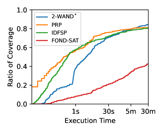
Table 11 shows part of the results. From it, we can verify that 2-WAND∗, PRP, and IDFSP have similar ratios of solved tasks, respectively 0.846, 0.812, and 0.808. FOND-SAT has 0.426. Figure 12 shows that if the time limit were around 5 minutes, then 2-WAND∗, PRP, and IDFSP would be basically tied regarding coverage. While 2-WAND∗ has a slower start in comparison to PRP and IDFSP, it shows slightly better scalability with more resources. Moreover, we note that we have verified that if we create a hybrid planner that runs PRP for 18 seconds, IDFSP for 22 seconds, and 2-WAND∗ for 115 seconds, this hybrid planner solves every task, achieving perfect coverage.
We note that the ratios for PRP in doors don’t sum to 100% in Table 11 because PRP concludes its execution failing to find a solution for doors’s p1, p2, and p3 instances. The column of failures by memory limit is missing for FOND-SAT because no execution of FOND-SAT has failed by memory out.
| PRP | 2-WAND∗ | ||
| Domain | |||
| blocksworld-original | 0.93 | 26.04 | 22.86 |
| blocksworld-advanced | 0.67 | 29.68 | 27.62 |
| earth-observation | 0.45 | 37.89 | 27.56 |
| elevators | 0.93 | 38.43 | 28.00 |
| first-responders | 0.97 | 15.77 | 14.78 |
| tireworld-triangle | 1.00 | 244.00 | 163.00 |
| zenotravel | 0.53 | 31.50 | 25.25 |
| miner | 0.27 | 17.71 | 16.14 |
| tireworld-truck | 0.31 | 22.39 | 12.83 |
| FOND-SAT | 2-WAND∗ | ||
| Domain | |||
| blocksworld-original | 0.33 | 10.10 | 10.20 |
| blocksworld-advanced | 0.24 | 9.92 | 10.46 |
| earth-observation | 0.12 | 8.80 | 8.40 |
| elevators | 0.47 | 14.86 | 15.29 |
| first-responders | 0.59 | 8.98 | 9.20 |
| zenotravel | 0.33 | 14.80 | 15.80 |
| miner | 0.47 | 16.04 | 16.33 |
| tireworld-truck | 0.85 | 13.46 | 13.90 |
We compare the (compressed) size of solutions returned by 2-WAND∗ with the size of solutions returned by PRP and FOND-SAT. We don’t compare with IDFSP because it reasons over states and returns solutions over states, while PRP and FOND-SAT reason over partial states and return solutions over partial states. Table 12a presents the comparison with PRP. The nine domains in the table are the ones with at least one task – among the ones solved by both 2-WAND∗ and PRP – with different returned solution sizes. Each row presents the average returned solution size of 2-WAND∗ and PRP for the entire intersection of tasks solved by both of them. Table 12b does the same, but for FOND-SAT.
We verify that there is no domain where 2-WAND∗ returns on average bigger solutions than PRP. It returns solution policies on average at least 10% smaller for six domains: blocksworld-original (12.2% smaller), earth-observation (27.3%), elevators (27.1%), tireworld-triangle (33.2%), zenotravel (20.0%), and tireworld-truck (42.7%). In the case of FOND-SAT, the sizes of solutions returned by 2-WAND∗ and FOND-SAT are very comparable. The difference in the average returned solution size was never more than 10% for a domain. Nevertheless, for seven domains, FOND-SAT returned on the average smaller solution, while for only one, earth-observation, it was the opposite. This is possible because, while FOND-SAT is expected, by design, to return compact solution partial policies, the SAT formulation it uses has some restrictions that may make it miss the minimal-sized solution partial policy. For the remaining eight domains, 2-WAND∗ and FOND-SAT have tied in this metric.
8 Conclusion and Future Work
In this work, we studied policy-space equivalence pruning. We verified that the policy-space search performed by AND∗ (Messa and Pereira, 2023) – a FOND planner that generalizes A∗ (Hart et al., 1968) for FOND planning – can be substantially improved with the use of equivalence pruning.
Throughout a deeper study of the structure of FOND policies, we presented three different features that can be used to derive equivalences between policies. We also presented a key procedure, called the concretizer, capable of finding the correct mappings of a solution in polynomial time if we know its states. The derived concepts of policy equivalences provide different guarantees and empirical improvements to the search performed by AND∗.
In this work, we also investigated other ideas to improve policy-space search. We show that taking into account symmetries over states allows a stronger and more effective pruning of policies, and that using a technique from the literature on group theory effectively allows an improved computation of symmetries over states that was previously recognized as intractable in practice. We also showed that while performing a greedy best-first policy-space search is detrimental, giving some reasonable extra weight to -values is beneficial.
We also presented a solution compressor that, given a policy defined over complete states, finds a policy that unambiguously represents it using the minimum number of partial states. The compressor allows the compression of solution policies found by any FOND planner using partial states. The compressor is time and memory-efficient for the benchmark tasks we solve and makes the solutions returned by AND∗ have state-of-the-art compactness in the majority of the benchmark domains.
In sum, this work advances the performance of policy-space explicit heuristic search by better understanding the structure of FOND policies. We investigate and incorporate techniques for detecting FOND policy and state symmetries. We also evaluate the use of satisficing search techniques and the compression of solutions. These contributions better explain the behavior of policy-space search and make the practical performance of AND∗ competitive to other well-established FOND planners. AND∗ with the presented improvements proved to be competitive against other state-of-the-art FOND planners both in terms of coverage and of solution compactness. We believe that our work, as a whole, allows a better understanding of how to design algorithms and heuristics to solve FOND tasks.
Future work includes studying better heuristics for policy-space search and how to use partial states to compress information during the search. This includes incorporating the idea of dead-end generalization from PRP and verifying its impact on this kind of search.
Another direction for future work is to better explore the potential of the concretizer. The concretizer has the potential to be useful even for projecting new FOND algorithms. In this work, we didn’t take advantage of the fact that we can deduce a solution from a domain set alone by calling the concretizer on , taking into account that we can compactly represent .
Acknowledgments
We thank UFRGS, CNPq, CAPES, and FAPERGS for partially funding this research. The present work was carried out with the support of CNPq, Conselho Nacional de Desenvolvimento Científico e Tecnológico - Brazil. We acknowledge support from FAPERGS with project 21/2551-0000741-9. This study was financed in part by the Coordenação de Aperfeiçoamento de Pessoal de Nível Superior - Brasil (CAPES) - Finance Code 001. We thank the authors of Winterer et al. (2016) for making their code available.
References
- Bäckström and Nebel (1995) Bäckström, C., Nebel, B., 1995. Complexity results for sas+ planning. Computational Intelligence 11, 625–655.
- Cimatti et al. (2003) Cimatti, A., Pistore, M., Roveri, M., Traverso, P., 2003. Weak, strong, and strong cyclic planning via symbolic model checking. Artificial Intelligence 147, 35–84.
- Doran and Michie (1966) Doran, J.E., Michie, D., 1966. Experiments with the graph traverser program, in: Proceedings of the Royal Society of London. Series A. Mathematical and Physical Sciences, pp. 235–259.
- Edelkamp and Schrödl (2011) Edelkamp, S., Schrödl, S., 2011. Heuristic Search: Theory and Applications. Elsevier.
- Fikes and Nilsson (1971) Fikes, R.E., Nilsson, N.J., 1971. Strips: A new approach to the application of theorem proving to problem solving. Artificial intelligence 2, 189–208.
- Geffner and Geffner (2018) Geffner, T., Geffner, H., 2018. Compact policies for fully observable non-deterministic planning as sat, in: Proceedings of the International Conference on Automated Planning and Scheduling, pp. 88–96.
- Hart et al. (1968) Hart, P.E., Nilsson, N.J., Raphael, B., 1968. A formal basis for the heuristic determination of minimum cost oaths. IEEE transactions on Systems Science and Cybernetics 4, 100–107.
- Helmert (2009) Helmert, M., 2009. Concise finite-domain representations for pddl planning tasks. Artificial Intelligence 173, 503–535.
- Helmert and Domshlak (2009) Helmert, M., Domshlak, C., 2009. Landmarks, critical paths and abstractions: what’s the difference anyway?, in: Proceedings of the International Conference on Automated Planning and Scheduling, pp. 162–169.
- Jefferson et al. (2019) Jefferson, C., Jonauskyte, E., Pfeiffer, M., Waldecker, R., 2019. Minimal and canonical images. Journal of Algebra 521, 481–506.
- McKay and Piperno (2014) McKay, B.D., Piperno, A., 2014. Practical graph isomorphism, ii. Journal of Symbolic Computation 60, 94–112.
- Messa and Pereira (2023) Messa, F., Pereira, A.G., 2023. A best-first search algorithm for fond planning and heuristic functions to optimize decompressed solution size, in: Proceedings of the International Conference on Automated Planning and Scheduling, pp. 277–285.
- Muise et al. (2012) Muise, C., McIlraith, S., Beck, C., 2012. Improved non-deterministic planning by exploiting state relevance, in: Proceedings of the International Conference on Automated Planning and Scheduling, pp. 172–180.
- Pereira et al. (2022) Pereira, R.F., Pereira, A.G., Messa, F., De Giacomo, G., 2022. Iterative depth-first search for fond planning, in: Proceedings of the International Conference on Automated Planning and Scheduling, pp. 90–99.
- Pochter et al. (2011) Pochter, N., Zohar, A., Rosenschein, J., 2011. Exploiting problem symmetries in state-based planners, in: Proceedings of the AAAI conference on artificial intelligence, pp. 1004–1009.
- Pohl (1970) Pohl, I., 1970. Heuristic search viewed as path finding in a graph. Artificial Intelligence 1, 193–204.
- Russell and Norvig (2016) Russell, S.J., Norvig, P., 2016. Artificial Intelligence: A Modern Approach. Pearson.
- Shleyfman et al. (2015) Shleyfman, A., Katz, M., Helmert, M., Sievers, S., Wehrle, M., 2015. Heuristics and symmetries in classical planning, in: Proceedings of the AAAI Conference on Artificial Intelligence, pp. 3371–3377.
- Winterer et al. (2016) Winterer, D., Wehrle, M., Katz, M., 2016. Structural symmetries for fully observable nondeterministic planning, in: Proceedings of the International Joint Conference On Artificial Intelligence, pp. 3293–3299.
Appendix A Proofs for AND∗ with Equivalence Pruning
In this section, we prove the theoretical guarantees AND∗ has under different settings of equivalence pruning. Proving that AND∗ always terminates and never returns if is not a solution (absence of false positives) is fairly straightforward. However, proving that it always returns an (optimal) solution when the given task is solvable (absence of false negatives) is challenging for most settings.
We present the concept of concept of (optimal) certificate pairs. The concept of (optimal) certificate pairs (Definitions 1) will be used to prove that AND∗ with certain settings always returns an (optimal) solution when the given task is solvable.
Weaker but sufficient concepts of heuristic admissibility and goal awareness (Messa and Pereira, 2023), are respectively implicitly asserted by the fourth and fifth requirements of optimal certificate pairs.
Definition 1
For a fixed given function and a fixed given solvable task , a pair of functions , with and for each possible policy is called a certificate pair iff:
-
1.
;
-
2.
For each policy , if , then either a solution is found when AND∗ analyzes , or such that ; and
-
3.
For each pair of policies and , if and , then and .
Such certificate pair is called optimal for a given heuristic function and a given cost metric iff additionally:
-
4.
For each policy , if , then for each solution ; and
-
5.
For each policy , if a solution is found when AND∗ analyzes , then .
A.1 General Proofs
In this subsection, we present the theoretical conclusions for AND∗ that are independent of the choice of .
Lemma 1
If takes a finite time to execute, then AND∗ always terminates.
Proof. The number of possible different policies is finite because the number of states and actions is finite. Therefore, the number of while-loop iterations is finite, since it is limited by the size of times the maximum number of successors ever generated during a policy expansion, which is finite. The initial setup takes a finite time, and similarly, each while-loop iteration since verifying if a policy is a solution and running the concretizer takes a finite amount of time (Lemma 6). Therefore AND∗ always terminates.
Lemma 2
AND∗ is sound when there is no solution.
Proof. By contraposition, assume it is not sound. Then, for some unsolvable task , it returns something different than . Such a return value cannot come from Line 10. However, then it is a solution, by the checks we do before other return statements. A direct contradiction with the unsolvability of .
Corollary 1
If takes a finite time to execute, then AND∗ always terminates and never returns false-positives.
Lemma 3
If, for some choice of , there exists some certificate pair for each solvable task, then AND∗ using this is sound when there is some solution.
Proof. By contraposition, assume it is not sound. Then, for some solvable task with some solution , it returns something different than a solution, despite the existence of some certificate pair . Such a return value can only come from Line 10, by the checks we do before other return statements. Thus, during AND∗ execution, all policies inserted in were eventually removed from it. Consider some policy with maximal that has and was once removed from (there is at least one, since ). If failed to meet after it was removed from , then there was another policy, , that was previously removed, with and the exact same and (granted by the third property of ), that did not fail to meet . In that case, we replace our initial choice of by , which is also a policy with maximal that has and was once removed from . Otherwise, we stick with the initial choice. Since our choice of meets , each was inserted in . At least one policy of such successors must have and due to the second property of . Such successor must have been removed from at some point, as all policies inserted in were eventually removed from it. Contradicting the fact that was a policy with maximal that has and was once removed from .
Corollary 2
If, in addition to Corollary 1 requirements, for some choice of , there exists some certificate pair for each solvable task, then AND∗ using this is sound and complete.
Lemma 4
If, for some choice of , there exists some optimal certificate pair for each solvable task for a given heuristic function and cost metric , then AND∗ using this is optimal for when guided by .
Proof. By contraposition, assume it is not optimal. Then, for some solvable task with some optimal solution , it returns some solution (by Lemma 3) when analyzing a policy , with , despite the existence of some optimal certificate pair . Since , by the fifth property of , all policies with inserted in were eventually removed from it, because of Line 3’s best-first choice. Therefore, all policies with inserted in were eventually removed from it, because they have , by the fourth property of . The remaining of the proof follows equal to Lemma 3’s proof. We consider some policy with maximal that has and was once removed from , and we reach a contradiction in the end.
Corollary 3
If, in addition to Corollary 2 requirements, the existent certificate pair is optimal for a heuristic function and cost metric , then AND∗ is additionally optimal for when guided by .
A.2 Equivalence Pruning Proofs
In this subsection, we present the theoretical conclusions for AND∗ using three different equivalence pruning signatures: identity (), lanes (), and domain-frontier (). We use a concept of heuristic extended awareness (Definition 2) to cope with the case where solutions come from the concretizer.
Definition 2
We say a FOND heuristic has extended awareness iff:
-
1.
, whenever is a solution; and
-
2.
whenever and .
Lemma 5
has extended awareness.
Proof. Whenever, for a pair of policies and , and , by design, since its computation considers only the , , and sets of a policy, not its mappings, and since in such conditions. Let be the solution that comes from the execution of the concretizer on . Then, and . Moreover, since is a solution, . Then, as well. Therefore, . Finally, as and . Therefore, . Thus,
A.2.1 Identity Equivalence Pruning
Theorem 1
AND∗ is sound and complete when , even without using the concretizer. Moreover, it is optimal for the cost metric when guided by a heuristic that is admissible and goal-aware to . This heuristic needs to have extended awareness if we use the concretizer.
Proof. Let be a solvable task, and be an arbitrary but fixed optimal solution policy . Let iff . Let . We show that the pair is an (optimal) certificate pair under the assumed circumstances.
-
1.
Trivially, .
-
2.
If, for some policy , , then . By contraposition, assume neither a solution is found when AND∗ analyzes nor such that . Since is a subset of a solution, it must be proper. But since no solution is found when AND∗ analyzes , then is not a solution although proper, thus . Then, such that for every action applicable to , . Note that such state must be in . Otherwise and would not be a solution. Let . Then is in and has and . Contradiction with the assumption that did not such that .
-
3.
If two policies and have , then given the choice of . Therefore and .
-
4.
If is a policy with , then and by ’s admissibility. Since is optimal, then for any solution .
-
5.
If is a solution, by ’s goal awareness. Otherwise, if the returned solution comes from the execution of the concretizer on , then , by ’s extended awareness. And , by ’s goal awareness.
A.2.2 Lanes Equivalence Pruning
Theorem 2
AND∗ is sound and complete, even without using the concretizer, when . Moreover, it is optimal for the cost metric of domain size when guided by an admissible and goal-aware optimal-size heuristic . This heuristic needs to have extended awareness if we use the concretizer.
Proof. Let be a solvable task, and be an arbitrary but fixed optimal solution policy . Let iff and , . Let . We show that the pair is an (optimal) certificate pair under the assumed circumstances.
-
1.
Since , then .
-
2.
If, for some policy , , then and . By contraposition, assume neither a solution is found when AND∗ analyzes nor such that . must be proper since as , as itself is proper as it is a subset of a solution. But, although proper, is not a solution since no solution is found when AND∗ analyzes . Then, such that for every action applicable to , . Note that such state must be in . Otherwise and would not be a solution. We prove this intermediate claim.
-
(a)
If , then , and either or .
-
(b)
Otherwise , then , then for at least one . Now, since , we have that . Consequently, . Then, either or .
Let . is in , has and . We now temporarily use notation to denote . We show that , . Let .
-
(a)
If and , then neither sets did change (i.e., and ). Therefore, .
-
(b)
If and , then and . Therefore, .
-
(c)
If , then and .
Therefore, . Contradiction with the assumption that did not such that .
-
(a)
-
3.
If two policies and have , then and for each state in their domain due to the choice of . Therefore and .
-
4.
It is easy to see that if, for some policy , , then there is some policy with and , from a repeated application of the second property, because it only stops when we reach a solution policy, and is optimal (thus there is no solution with smaller domain set). is an optimal solution. since is an admissible optimal-size heuristic. And since is optimal, for any solution .
-
5.
If is a solution, by ’s goal awareness. Otherwise, if the returned solution comes from the execution of the concretizer on , then , by ’s extended awareness. And , by ’s goal awareness.
A.2.3 Domain-Frontier Equivalence Pruning
Theorem 3
AND∗ is sound and complete when it is using the concretizer and . Moreover, it is optimal for the cost metric of domain size when guided by an admissible and goal-aware optimal-size heuristic that has extended awareness.
Proof. Let be a solvable task, and be an arbitrary but fixed optimal solution policy . Let iff with and . Let . We show that the pair is an (optimal) certificate pair under the assumed circumstances.
-
1.
Since , then .
-
2.
If, for some policy , , then with and . By contraposition, assume neither a solution is found when AND∗ analyzes nor such that . Since no solution is found when AND∗ analyzes , then is not a solution and either or the concretizer returned for . However, the latter couldn’t have happened because of the existence of , which is proper as it is a subset of a solution, so must be the case. Then, such that for every action applicable to , . Note that such state must be in , as it is in and . Otherwise and would not be a solution. Let . is in and has . Moreover, let . and . Therefore, . Contradiction with the assumption that did not such that .
-
3.
If two policies and have , then we have due to the choice of . Therefore, and .
-
4.
If, for some policy , , then with and . Note that , since has extended awareness. Then, since is an admissible optimal-size heuristic. And since is optimal, then for any solution .
-
5.
If is a solution, by ’s goal awareness. Otherwise, if the returned solution comes from the execution of the concretizer on , then , by ’s extended awareness. And , by ’s goal awareness.
Appendix B Concretizer Theoretical Proofs
Lemma 6
The concretizer always terminates.
Proof. At each iteration, either the concretizer ends returning , or it decreases the size of by one. Therefore, the number of iterations is finite (as we assume hollow policies are pairs of finite sets). Then, since each instruction takes a finite time, each execution of the concretizer must eventually terminate.
Lemma 7
If the concretizer returns a policy , then it is proper, , and .
Proof. The return must have occurred at Line 14. We show by induction on the iterations of the concretizer that had , and (implying properness) throughout the entire execution. By proving that, we will achieve the desired conclusion, taking into account that when Line 14 is reached, , and therefore .
-
1.
Before the first iteration, the hypothesis is trivially true since .
-
2.
We show that if, at the beginning of an iteration, the hypothesis is true, then it must also be at the end of that iteration. Since was never returned, the if-statement was satisfied at each iteration.
-
(a)
If then by choice of .
-
(b)
If then by choice of and with .
-
(c)
If each -reaches a state in , then each -reaches a state in by choice of and with (since ).
-
(a)
Lemma 8
The concretizer is sound when there is no proper policy with and .
Proof. By contraposition, assume it is not sound. Then, for some input for which there is no proper policy with and , it returns something different than (otherwise it would be sound). Thus, it returns some policy at Line 14. Then, by applying Lemma 7, we obtain a contradiction with our assumption of the nonexistence of a proper policy with and .
Lemma 9
The concretizer is sound when there some proper policy with and .
Proof. By contraposition, assume it is not sound. Then, for some input for which there is some proper policy with and , it returns something different than a policy with such properties. Then, by Lemma 7, it must have returned no policy at all. The only alternative is that it returned at Line 13. Then, at the beginning of some iteration it occurred that didn’t exist and with applicable to , , and . We show that that couldn’t have occurred under the current assumptions. Let . Since and is proper, is proper. Therefore and such that . We choose such a state and action , and we note that because and (by construction of ). Moreover, since and , then it must be true that . Therefore exists and applicable to , with and . Contradiction.
Theorem 4
The concretizer is sound and complete.
Appendix C Glossary of Symbols and Functions
-
The set of facts, which might be either true or false in a state.
-
The set of facts that are true in the state .
-
The set of states.
-
The set of goal states.
-
The set of actions.
-
The set of all states that might be achieved if we apply the action at the state . Also called the successor states of through .
-
A partial function that maps non-goal states to actions. It is called a policy.
-
The action that is mapped to in . iff is not mapped in .
-
The set of states mapped in – i.e., the domain of .
-
The set of states reachable from some state in through the use of actions in . This set includes the domain states themselves.
-
Equal to . A state in is called a frontier state of .
-
Equal to plus the initial state if it is non-goal and is not in the domain of the policy. A proper policy is a solution iff is empty.
-
The set of states reachable from through the use of actions in . This set includes itself.
-
Equal to . Also equal to . A policy is proper iff, for each domain state , this set is not empty.
-
Operation that returns a policy , such that if , and otherwise.