On Quantile Randomized Kaczmarz for Linear Systems with Time-Varying Noise and Corruption

Abstract.

Large-scale systems of linear equations arise in machine learning, medical imaging, sensor networks, and in many areas of data science. When the scale of the systems are extreme, it is common for a fraction of the data or measurements to be corrupted. The Quantile Randomized Kaczmarz (QRK) method is known to converge on large-scale systems of linear equations $A{\mathbf{x}}={\mathbf{b}}$ that are inconsistent due to static corruptions in the measurement vector ${\mathbf{b}}$. We prove that QRK converges even for systems corrupted by time-varying perturbations. Additionally, we prove that QRK converges up to a convergence horizon on systems affected by time-varying noise and demonstrate that the noise affects only the convergence horizon of the method, and not the rate of convergence. Finally, we utilize Markov’s inequality to prove a lower bound on the probability that the largest entries of the QRK residual reveal the time-varying corruption in each iteration. We present numerical experiments which illustrate our theoretical results.

1. Introduction

Solving large-scale systems of linear equations is one of the most commonly encountered problems across the data-rich sciences. This problem arises in machine learning, as subroutines of several optimization methods [5], in medical imaging [13, 16], in sensor networks [37], and in statistical analysis, to name only a few. Stochastic or randomized iterative methods have become increasingly popular approaches for a variety of large-scale data problems as these methods typically have low-memory footprint and are accompanied by attractive theoretical guarantees. Indeed, the scale of modern problems often make application of direct or non-iterative methods challenging or infeasible [36]. Examples of randomized iterative methods which have found popularity in recent years include the stochastic gradient descent method [34] and the randomized Kaczmarz method [40].

Large-scale data, where iterative methods typically find superiority over direct methods, nearly always suffers from corruption – from error in measurement or data collection, in storage, in transmission and retrieval, and in data handling. In this work, we consider solving linear problems where a few measurements or components have been subjected to corruptions that disrupt solution by usual techniques. Problems in which a small number of untrustworthy data can have a devastating effect on a variable of interest have been considered in  [2, 19, 6, 9]. In particular, linear problems with a small number of outlier measurements have led to an interest in methods for robust linear regression [35, 43, 3]. Other relevant work includes min-k loss SGD [38], robust SGD [10, 33], and Byzantine approaches [4, 1].

In application areas where robust linear regression and robust numerical linear algebra are most impactful, data perturbations are often introduced in a streaming and non-static manner (e.g., during distributed data access [21]). For example, when solving a system of linear equations that is large enough to be distributed amongst various storage servers, accessing subgroups of equations at different times from these servers may introduce a varying amount of noise and corruption (or none) into the accessed measurement; a single equation could be corrupted or noisy in one access but not in another. The previously considered model of static corruption in the measurement vector is no longer sufficient; the measurement vector, noise, and corruption should be modeled in a time-varying manner.

1.1. Problem set-up

In this paper, we consider solving highly overdetermined linear systems which are perturbed by both noise and corruption that vary with time. We are considering the situation in which we have a matrix $A\in\mathbb{R}^{m\times n}$ and a vector ${\mathbf{b}}\in\mathbb{R}^{m}$ which define a highly overdetermined consistent system $A{\mathbf{x}}={\mathbf{b}}$, with $m\gg n$. We assume the measurement matrix is full-rank, $\text{rank}(A)=n$, and let ${\mathbf{x}}^{*}\in\mathbb{R}^{n}$ denote the solution to the consistent system $A{\mathbf{x}}^{*}={\mathbf{b}}$. We will represent the noise and corruption as time-varying vectors sampled in each iteration ${\mathbf{n}}^{(k)}\in\mathbb{R}^{m}$ and ${\mathbf{c}}^{(k)}\in\mathbb{R}^{m}$, respectively. These vectors obscure the true value of ${\mathbf{b}}$, creating the observed, time-varying measurement vector ${\mathbf{b}}^{(k)}={\mathbf{b}}+{\mathbf{n}}^{(k)}+{\mathbf{c}}^{(k)}$. We assume that the values of ${\mathbf{b}},{\mathbf{n}}^{(k)},$ and ${\mathbf{c}}^{(k)}$ are not known and only ${\mathbf{b}}^{(k)}$ is observed. We assume that the number of corruptions is no more than a fraction $0<\beta\ll 1$ of the total number of measurements, $\|{\mathbf{c}}^{(k)}\|_{\ell_{0}}:=|\text{supp}({\mathbf{c}}^{(k)})|\leq\beta m$. Here $\text{supp}({\mathbf{x}})$ denotes the set of indices of nonzero entries of ${\mathbf{x}}$. We define the set of corrupted equations in the $k$th iteration to be $C_{k}=\text{supp}({\mathbf{c}}^{(k)})\subset\{1,2,\dots,m\}.$

1.2. Organization

The remainder of our paper is organized as follows. We discuss related works in Section 1.3, define relevant notation and state our assumptions in Section 1.4, provide detailed pseudocode of the quantile randomized Kaczmarz (QRK) method in Section 1.5, and present our main contributions in Section 1.6. In Section 2 we present statements and proofs of our theoretical results, and in Section 3 we empirically demonstrate our theoretical results with numerical experiments on synthetic data. Finally, we provide some conclusions and discussion in Section 4.

1.3. Related work

Kaczmarz methods, a classical example of row-action iterative methods, consist of sequential orthogonal projections towards the solution set of a single equation [18]; the $j$th iterate is recursively defined as

(1) $${\mathbf{x}}^{(j)}={\mathbf{x}}^{(j-1)}-\frac{{\mathbf{a}}_{i_{j}}^{T}{\mathbf{x}}^{(j-1)}-b_{i_{j}}}{\|{\mathbf{a}}_{i_{j}}\|^{2}}{\mathbf{a}}_{i_{j}}$$

where ${\mathbf{a}}_{i_{j}}$ is the $i_{j}$th row of $A$, $b_{i_{j}}$ is the $i_{j}$th entry of ${\mathbf{b}}$, and $i_{j}\in\{1,2,\cdots,m\}$ is the equation selected in the $j$th iteration. These methods saw a renewed surge of interest after the elegant convergence analysis of the Randomized Kaczmarz (RK) method in [40]; the authors showed that for a consistent system with unique solution ${\mathbf{x}}^{*}$, RK (where $i_{j}=l$ with probability $\|{\mathbf{a}}_{l}\|^{2}/\|A\|_{F}^{2}$) converges at least linearly in expectation with the guarantee

(2) $$\mathbb{E}\|{\mathbf{x}}^{(k)}-{\mathbf{x}}^{*}\|^{2}\leq\left(1-\frac{\sigma_{\min}^{2}(A)}{\|A\|_{F}^{2}}\right)^{k}\|{\mathbf{x}}^{(0)}-{\mathbf{x}}^{*}\|^{2},$$

where $\sigma_{\min}(A)$ is the minimum singular-value of the matrix $A$. Many variants and extensions followed, including convergence analyses for inconsistent and random linear systems [27, 7], connections to other popular iterative algorithms [23, 28, 30, 31, 11], block approaches [29, 32], acceleration and parallelization strategies [12, 22, 26, 25], and techniques for reducing noise [44].

A recent line of work has introduced quantile statistics of the in-iteration residual information into randomized iterative methods to detect and avoid corrupted data in large-scale linear systems [15]. These problems arise in medical imaging, sensor networks, error correction and data science, where effects of adversarial corruptions in the data could be catastrophic down-stream. An ill-timed update using corrupted data can destroy the valuable information learned by many updates produced with uncorrupted data, making iterative methods challenging to employ on large-scale data; see Figure 1 for an example of the effect of corrupted data on an iterative method for solving linear systems. The quantile randomized Kaczmarz (QRK) method is a variant of the Kaczmarz method designed to avoid the impacts of a small number of corruptions in the measurement vector. QRK differs from RK in that, in each iteration, the usual Kaczmarz projection step is only taken if the sampled residual entry magnitude is less than a sufficient fraction of residual entry magnitudes, indicating that this sampled equation is likely not affected by a corruption. QRK is known to converge in expectation to the solution to the uncorrupted system ${\mathbf{x}}$ under mild assumptions [15, 39, 17, 8, 14]. By ensuring that updates are generated using only data with residual magnitude less than a sufficiently-small quantile statistic of the entire residual, QRK can avoid updates corresponding to highly corrupted data. In this paper, we show that QRK converges in the more general case that the system is affected by time-varying corruption and noise.

Figure 1. A linear system in which some equations (blue) have been corrupted and two iterations of a Kaczmarz method.

The setting of time-varying and random noise in the system measurements has been considered previously in the Kaczmarz literature. In [24], the authors consider the scenario that the measurements, ${\mathbf{b}}$, of a consistent system are perturbed by independent mean zero random noise with bounded variance, and derive an optimal learning rate (or relaxation parameter) schedule for the randomized Kaczmarz method which minimizes the expected error. In [42], the authors consider an independent noise model in which, each time the system is sampled, the entries of the sample are assumed to be perturbed by freshly sampled independent mean zero random noise values with bounded variance, and derive adaptive step sizes that allow the block Bregman-Kaczmarz method to converge to the solution of the unperturbed system. Both of these works develop methods which converge to the solution of the unperturbed (no noise) system, breaking the so-called convergence horizon suffered by the standard RK method applied to systems with noise [27]. On the other hand, our paper will be concerned with quantifying the effect of general time-varying noise and corruption on the convergence horizon and rate of QRK.

1.4. Notation and assumptions

We will use boldfaced lower-case Latin letters (e.g., ${\mathbf{x}}$) to denote vectors and unbolded upper-case Latin letters (e.g., $A$) to denote matrices. We use unbolded lower-case Latin and Roman letters (e.g., $q$ and $\beta$) to denote scalars. We let $[m]$ denote the set $\{1,2,\cdots,m\}$. If $A$ is an $m\times n$ matrix and $S\subset[m],$ then let $A_{S}$ denote the matrix obtained by restricting to the rows indexed by $S$ and let $A_{\not\in S}$ denote the matrix obtained by removing from $A$ the rows indexed by $S$. We denote the $i$th row of $A$ by ${\mathbf{a}}_{i}\in\mathbb{R}^{n}$ for $i\in[m]$. We let $q\text{-quant}\left(S\right)$ denote the empirical $q$-quantile of a multi-set $S$; that is the $\lfloor q|S|\rfloor^{\text{th}}$ smallest entry of $S$.

The notation $\|{\mathbf{v}}\|$ denotes the Euclidean norm of a vector ${\mathbf{v}}$. All other $p$-norms of vectors ${\mathbf{v}}$ are denoted with subscript, $\|{\mathbf{v}}\|_{p}$.

For a matrix $A$, we denote its operator ($L_{2}\to L_{2}$) norm by $\|A\|=\sup_{{\mathbf{x}}\in S^{n-1}}\|A{\mathbf{x}}\|$ and its Frobenious (or Hilbert-Schmidt) norm by $\|A\|_{F}=\sqrt{\operatorname{trace}(A^{\top}A)}$. Throughout, we denote by $\sigma_{\text{min}}(A)$ and $\sigma_{\max}(A)$ the smallest and largest singular values of the matrix $A$ (that is, eigenvalues of the matrix $\sqrt{A^{\top}A}$). Moreover, we always assume that the matrix $A$ has full column rank, so that $\sigma_{\min}(A)>0$.

Our convergence analyses involve several random variables; the random sample of index in the $k$th iteration, $i_{k}$, and in some cases, the random noise introduced into the system measurements in the $k$th iteration, ${\mathbf{n}}^{(k)}$.

We will be interested in $\mathbb{E}_{i_{k}}\|{\mathbf{x}}^{(k+1)}-{\mathbf{x}}^{*}\|^{2}$ which is the expectation of the squared error of ${\mathbf{x}}^{(k+1)}$ with respect to the sampled index in the $k$th iteration, $i_{k}$, where the sampling is according to the distribution in context, i.e., the Kaczmarz sampling distribution.

We will also be interested in $\mathbb{E}_{i_{k}}\left[\|{\mathbf{x}}^{(k+1)}-{\mathbf{x}}^{*}\|^{2}\;|\;i_{k}\in S_{k}\right]$ which is the conditional expectation of the squared error of ${\mathbf{x}}^{(k+1)}$ with respect to the sampled index in the $k$th iteration, $i_{k}$, conditioned upon $i_{k}\in S_{k}$, where the sampling is according to the distribution in context, i.e., the Kaczmarz sampling distribution.

We’ll let $\mathbb{E}_{i_{1},\cdots,i_{k}}\|{\mathbf{x}}^{(k+1)}-{\mathbf{x}}^{*}\|^{2}$ denote the iterated expectation with respect to all sampled indices and will let $\mathbb{E}\|{\mathbf{x}}^{(k+1)}-{\mathbf{x}}^{*}\|^{2}$ denote the expectation with respect to the joint distribution of all random variables.

Our convergence results will hinge upon a submatrix conditioning parameter introduced in [39]; we define

(3) $$\sigma_{q-\beta,\min}(A)=\min_{\begin{subarray}{c}S\subset[m]\\ |S|=\lfloor(q-\beta)m\rfloor\end{subarray}}\inf_{\|{\mathbf{x}}\|=1}\|A_{S}{\mathbf{x}}\|.$$

This parameter measures the smallest singular value encountered in any submatrix determined by a $q-\beta$-fraction of the rows of $A$. Our results will also depend upon three parameters which determine the convergence rate and convergence horizon; we define these terms in Definition 1.1.

Definition 1.1.

We define a rate parameter,

$$\varphi=\frac{\sigma_{q-\beta,\text{{min}}}^{2}(A)}{qm}\bigg{(}\frac{q-\beta}{q}\bigg{)}-\frac{\sigma_{\text{{max}}}^{2}(A)}{qm}\bigg{(}\frac{2\sqrt{\beta(1-\beta)}}{(1-q-\beta)}+\frac{\beta(1-\beta)}{(1-q-\beta)^{2}}\bigg{)}-\frac{\sigma_{\text{{max}}}(A)}{qm}\bigg{(}\frac{2\sqrt{\beta m}}{m(1-q-\beta)}+\frac{2\beta\sqrt{m(1-\beta)}}{m(1-q-\beta)^{2}}\bigg{)},$$

a parameter governing the influence of the quantile and corruption rate on the convergence horizon,

$$\zeta=\frac{\sigma_{\text{{max}}}(A)}{qm}\bigg{(}\frac{2\sqrt{\beta m}}{m(1-q-\beta)}+\frac{2\beta\sqrt{m(1-\beta)}}{m(1-q-\beta)^{2}}\bigg{)}+\frac{\beta}{qm^{2}(1-q-\beta)^{2}},$$

and a parameter measuring the convergence horizon,

$$\gamma_{k}=\sum_{j=0}^{k}(1-p\varphi)^{k-j}\left(\frac{\lVert{\mathbf{n}}_{B_{j}\setminus S_{j}}^{(j)}\rVert_{2}^{2}}{\lVert A_{B_{j}\setminus S_{j}}\rVert_{F}^{2}}+\zeta\lVert{\mathbf{n}}^{(j)}\rVert_{1}^{2}\right).$$

Here, $S_{j}\subseteq B_{j}\subseteq[m]$ are sets defined below.

We list next two assumptions made throughout this paper.

Assumption 1.2.

The matrix $A\in\mathbb{R}^{m\times n}$ has rows with unit norm, $\|{\mathbf{a}}_{i}\|=1$ for all $i\in[m]$.

Assumption 1.3.

The rate parameter is positive, $\varphi>0$.

1.5. Quantile randomized Kaczmarz

As mentioned previously, QRK is a variant of RK where, in each iteration, the update is made only if the sampled residual entry magnitude is less than a sufficient fraction of residual entry magnitudes. The algorithm uses this residual magnitude comparison as a proxy indicator for whether it is affected by a corruption.

Practically, there are two implementations of the QRK algorithm. In the first, we randomly sample from the entire residual and only make the update if the sampled residual magnitude is less than a sufficient fraction of the other residual entry magnitudes. Pseudocode for this implementation is given in Algorithm 1; this implementation is due to [15]. In the second, we randomly sample only from the residual entries whose magnitude is less than a sufficient fraction of the other residual entry magnitudes and make the update in each iteration. Pseudocode for this implementation is given in Algorithm 2; this implementation is due to [39].

Algorithm 1 QuantileRK [15]

1:procedure QuantileRK1($A,{\mathbf{b}}$, ${\mathbf{x}}^{(0)}$, q, N)

2:     for j = 1, …, N do

3:         sample $i_{j}\sim\text{Unif}([m])$

4:         if  $\left|\left\langle{\mathbf{a}}_{i_{j}},{\mathbf{x}}^{(j-1)}\right\rangle-b_{i_{j}}\right|\leq q\text{-quant}\left(\left\{\left|\left\langle{\mathbf{a}}_{i},{\mathbf{x}}^{(j-1)}\right\rangle-b_{i}\right|\right\}_{i=1}^{m}\right)$ then

5:              ${\mathbf{x}}^{(j)}={\mathbf{x}}^{(j-1)}-\frac{\left(\left\langle{\mathbf{a}}_{i_{j}},{\mathbf{x}}^{(j-1)}\right\rangle-b_{i_{j}}\right)}{\|{\mathbf{a}}_{i_{j}}\|^{2}}{\mathbf{a}}_{i_{j}}$

6:         else

7:              ${\mathbf{x}}^{(j)}={\mathbf{x}}^{(j-1)}$                return ${\mathbf{x}}^{(N)}$

Algorithm 2 QuantileRK [39]

1:procedure QuantileRK2($A,{\mathbf{b}}$, ${\mathbf{x}}^{(0)}$, q, N)

2:     for j = 1, …, N do

3:         sample $i_{j}\sim\text{Unif}\left(\left\{l:\left|\left\langle{\mathbf{a}}_{l},{\mathbf{x}}^{(j-1)}\right\rangle-b_{l}\right|\leq q\text{-quant}\left(\left\{\left|\left\langle{\mathbf{a}}_{i},{\mathbf{x}}^{(j-1)}\right\rangle-b_{i}\right|\right\}_{i=1}^{m}\right)\right\}\right)$

4:         ${\mathbf{x}}^{(j)}={\mathbf{x}}^{(j-1)}-\frac{\left(\left\langle{\mathbf{a}}_{i_{j}},{\mathbf{x}}^{(j-1)}\right\rangle-b_{i_{j}}\right)}{\|{\mathbf{a}}_{i_{j}}\|^{2}}{\mathbf{a}}_{i_{j}}$       return ${\mathbf{x}}^{(N)}$

These implementations may be analyzed in the same way; we will provide a convergence analysis valid for both in Theorem 1.4 and provide a proof in Section 2.

1.6. Main contributions

In this section, we list our main results. Our first main result proves that QRK converges at least linearly in expectation up to a convergence horizon even in the case of time-varying corruption and noise. We note that the rate of convergence depends only upon parameters determined by the time-varying corruption, in particular the corruption rate, while the convergence horizon depends upon both the corruption rate and the time-varying noise in the system.

Theorem 1.4.

Let ${\mathbf{x}}^{(k)}$ denote the iterates of Algorithm 1 or Algorithm 2 applied with quantile $q$ to the system defined by $A$ and ${\mathbf{b}}^{(k)}={\mathbf{b}}+{\mathbf{n}}^{(k)}+{\mathbf{c}}^{(k)}$, in the $k$th iteration. Assuming the setup described in Section 1.1, Assumptions 1.2 and 1.3, and $\beta<q<1-\beta$ arbitrary, then

$$\mathbb{E}_{\;}\lVert{\mathbf{x}}^{(k+1)}-{\mathbf{x}}^{*}\rVert^{2}\leq(1-p\varphi)^{k+1}\lVert{\mathbf{x}}^{(0)}-{\mathbf{x}}^{*}\rVert^{2}+p\gamma_{k},$$

where $p$ represents the probability that a row is selected from within the $q$-quantile in each iteration, and $\varphi$ and $\gamma_{k}$ are as given in Definition 1.1.

In Corollary 1.4.1, we take stronger assumptions on the form of the noise. In Corollary 1.4.1 (a), we specialize Theorem 1.4 to the case that the noise in each iteration is uniformly bounded. In Corollary 1.4.1 (b), we specialize Theorem 1.4 to the case that the noise is sampled from a known distribution, and in Corollary 1.4.1 (c), we specialize to the case that the noise has entries sampled from a Gaussian distribution.

Corollary 1.4.1.

Let ${\mathbf{x}}^{(k)}$ denote the iterates of Algorithm 1 or Algorithm 2 applied with quantile $q$ to the system defined by $A$ and ${\mathbf{b}}^{(k)}={\mathbf{b}}+{\mathbf{n}}^{(k)}+{\mathbf{c}}^{(k)}$, in the $k$th iteration. We assume the setup described in Section 1.1, Assumptions 1.2 and 1.3, and $\beta<q<1-\beta$ arbitrary. We let $p$ be the probability that a row is selected from within the $q$-quantile in each iteration, and $\varphi$ and $\zeta$ are as given in Definition 1.1.

1. If $n_{max}\geq|n^{(j)}_{i}|$ for all $j\in[k+1]$ and $i\in[m]$, then

   $$\mathbb{E}_{i_{1},\cdots,i_{k}}\|{\mathbf{x}}^{(k+1)}-{\mathbf{x}}^{*}\|^{2}\leq(1-p\varphi)^{k+1}\lVert{\mathbf{x}}^{(0)}-{\mathbf{x}}^{*}\rVert^{2}+(1+\zeta m^{2})(n_{max})^{2}\frac{1-(1-p\varphi)^{k+1}}{\varphi}.$$

2. If $n_{i}^{(k)}$ are i.i.d samples from distribution with mean $\mu$ and standard deviation $\sigma$, and the mean and standard deviation of $|n_{i}^{(k)}|$ are $\mu^{\prime}$ and $\sigma^{\prime}$, respectively, then

   $$\mathbb{E}\|{\mathbf{x}}^{(k+1)}-{\mathbf{x}}^{*}\|^{2}\leq(1-p\varphi)^{k+1}\lVert{\mathbf{x}}^{(0)}-{\mathbf{x}}^{*}\rVert^{2}+\frac{1-(1-p\varphi)^{k+1}}{\varphi}\left({\mu^{2}+\sigma^{2}}+\zeta[m^{2}(\mu^{\prime})^{2}+m(\sigma^{\prime})^{2}]\right).$$

3. If $n_{i}^{(k)}$ are i.i.d samples from $\mathcal{N}(0,\sigma^{2})$, then

   $$\mathbb{E}\|{\mathbf{x}}^{(k+1)}-{\mathbf{x}}^{*}\|^{2}\leq(1-p\varphi)^{k+1}\lVert{\mathbf{x}}^{(0)}-{\mathbf{x}}^{*}\rVert^{2}+\frac{1-(1-p\varphi)^{k+1}}{\varphi}\sigma^{2}(1+\zeta[m^{2}\frac{2}{\pi}+m(1-\frac{2}{\pi})]).$$

Our final main result utilizes Theorem 1.4 to provide a lower bound on the probability that the indices of the corrupted equations in the $k$th iteration are given by examining the $k$th residual and identifying the $\lfloor\beta m\rfloor$ largest entries. That is, even in the case that the corruption indices are changing and the system is perturbed by time-varying noise, the largest entries of the residual reveal the position of the corruptions.

Corollary 1.4.2.

Let ${\mathbf{x}}^{(k)}$ denote the iterates of Algorithm 1 or Algorithm 2 applied with quantile $q$ to the system defined by $A$ and ${\mathbf{b}}^{(k)}={\mathbf{b}}+{\mathbf{n}}^{(k)}+{\mathbf{c}}^{(k)}$, in the $k$th iteration. Let $n_{max}$ be the value that satisfies $n_{max}\geq|n^{(j)}_{i}|$ for all $1\leq j\leq k+1$ and for all $i\in[m]$, and $\varphi$ and $\zeta$ are as given in Definition 1.1. Define $c^{(k)}_{\min}=\min_{i\in\text{supp}({\mathbf{c}}^{(k)})}|c_{i}^{(k)}|,$ and assume $(1+\zeta m^{2})\frac{n_{\max}^{2}}{\varphi}\leq(c_{\min}^{(k)})^{2}/4M$ for some value $M\gg 1$. Assuming the setup described in Section 1.1, Assumptions 1.2 and 1.3, and $\beta<q<1-\beta$ arbitrary, then with probability at least

$$\frac{M-1}{M}-\frac{4(1-p\varphi)^{k}\|{\mathbf{x}}^{(0)}-{\mathbf{x}}^{*}\|^{2}}{(c^{(k)}_{\min})^{2}}$$

where $p$ represents the probability that a row is selected from within the $q$-quantile in each iteration, we have that by iteration $k$, the (time-varying) position of the corruptions can be identified by evaluating the residual and identifying the $\beta m$ largest entries; that is,

$$\text{supp}({\mathbf{c}}^{(k)})\subset\text{argmax}_{\begin{subarray}{c}S\subset[m],\\ |S|=\lfloor\beta m\rfloor\end{subarray}}\sum_{i\in S}|{\mathbf{a}}_{i}^{\top}{\mathbf{x}}^{(k)}-b_{i}^{(k)}|.$$

Remark.

In the noiseless case, when ${\mathbf{n}}^{(k)}=\mathbf{0}$ for all iterations $k$, Corollary 1.4.2 holds with probability at least

$$1-\frac{4(1-p\varphi)^{k}\|{\mathbf{x}}^{(0)}-{\mathbf{x}}^{*}\|^{2}}{(c^{(k)}_{\min})^{2}}.$$

2. Theoretical Results

In this section, we provide proofs of our main results. In Section 2.1, we provide a convergence analysis for the randomized Kaczmarz method [41] on a system perturbed by time-varying noise with entries sampled i.i.d.  from a distriution with mean $\mu$ and standard deviation $\sigma$. This result will be utilized as a lemma in several of our other proofs, but may be of independent interest. In Section 2.2, we prove our main result, Theorem 1.4, and in Section 2.3, we prove the corollaries of our main result, Corollary 1.4.1 and Corollary 1.4.2.

2.1. Convergence of RK on systems with time-varying noise

Our convergence analysis of QRK will hinge upon the approach taken in analyzing the randomized Kaczmarz method in the case that the system of interest is perturbed by time-varying noise. This result, while useful as a lemma to us, is of independent interest.

Theorem 2.1.

Let $A\in\mathbb{R}^{m\times n}$ with $m>n$ and ${\mathbf{b}}\in\mathbb{R}^{m}$ define a consistent system $A{\mathbf{x}}^{*}={\mathbf{b}}$ with unique solution ${\mathbf{x}}^{*}\in\mathbb{R}^{n}$. Let ${\mathbf{x}}^{(k)}$ denote the iterates of the randomized Kacmzarz method [41] applied to the system defined by $A$ and ${\mathbf{b}}^{(k)}={\mathbf{b}}+{\mathbf{n}}^{(k)}$ in the $k$ iteration.

If $n_{i}^{(k)}$ are i.i.d samples from a distribution with mean $\mu$ and standard deviation $\sigma$, then the error decreases at least linearly in expectation with

$$\mathbb{E}\|{\mathbf{x}}^{(k+1)}-{\mathbf{x}}^{*}\|^{2}\leq\phi^{k+1}\|{\mathbf{x}}^{(0)}-{\mathbf{x}}^{*}\|^{2}+\frac{1-\phi^{k+1}}{1-\phi}\frac{m}{\|A\|^{2}_{F}}(\sigma^{2}+\mu^{2})$$

where

$$\phi=1-\frac{\sigma_{min}^{2}(A)}{\|A\|^{2}_{F}}.$$

Figure 2. An illustration of the errors of the iterates ${\mathbf{x}}^{(k+1)}$ and $\hat{{\mathbf{x}}}^{(k+1)}$ produced from ${\mathbf{x}}^{(k)}$ on the noisy and noiseless systems, respectively.

Proof.

Consider two instances of the randomized Kaczmarz method producing iterates $\{{\mathbf{x}}^{(k)}\}$ and $\{\hat{{\mathbf{x}}}^{(k)}\}$. One sequence of iterates, $\{{\mathbf{x}}^{(k)}\}$, is generated using the time varying system defined by $A$ and ${\mathbf{b}}^{(k)}={\mathbf{b}}+{\mathbf{n}}^{(k)}$, and the other, $\{\hat{{\mathbf{x}}}^{(k)}\}$ using the unobserved noiseless system defined by $A$ and ${\mathbf{b}}$, both with the same sequence of row selections $\{i_{k}\}$. As illustrated in the diagram in Figure 2, the Pythagorean theorem implies

(4) $$\|{\mathbf{x}}^{(k)}-{\mathbf{x}}^{*}\|^{2}=\|{\mathbf{x}}^{(k)}-\hat{{\mathbf{x}}}^{(k+1)}\|^{2}+\|\hat{{\mathbf{x}}}_{(k+1)}-{\mathbf{x}}^{*}\|^{2},$$

and

(5) $$\|{\mathbf{x}}^{(k+1)}-{\mathbf{x}}^{*}\|^{2}=\|\hat{{\mathbf{x}}}^{(k+1)}-{\mathbf{x}}^{*}\|^{2}+\|\hat{{\mathbf{x}}}^{(k+1)}-{\mathbf{x}}^{(k+1)}\|^{2}.$$

We now observe that the quantity $\|\hat{{\mathbf{x}}}^{(k+1)}-{\mathbf{x}}^{(k+1)}\|$ represents the difference between a non-noisy and noisy iteration of Kaczmarz, where both use ${\mathbf{x}}^{(k)}$ as the previous iterate. Then

$${\|\hat{{\mathbf{x}}}^{(k+1)}-{\mathbf{x}}^{(k+1)}\|} = \left\|{\mathbf{x}}^{(k)}+\frac{b_{i_{k}}-{\mathbf{a}}_{i_{k}}^{T}{\mathbf{x}}^{(k)}}{\|{\mathbf{a}}_{i_{k}}\|^{2}}{\mathbf{a}}_{i_{k}}-\left({\mathbf{x}}^{(k)}+\frac{b_{i_{k}}+n^{(k)}_{i_{k}}-{\mathbf{a}}_{i_{k}}^{T}{\mathbf{x}}^{(k)}}{\|{\mathbf{a}}_{i_{k}}\|^{2}}{\mathbf{a}}_{i_{k}}\right)\right\|=\frac{|n^{(k)}_{i_{k}}|}{\|{\mathbf{a}}_{i_{k}}\|}.$$

Meanwhile, the quantity $\|{\mathbf{x}}^{(k)}-\hat{{\mathbf{x}}}^{(k+1)}\|$ is

$${\|{\mathbf{x}}^{(k)}-\hat{{\mathbf{x}}}^{(k+1)}\|} = \left\|{\mathbf{x}}^{(k)}-\left({\mathbf{x}}^{(k)}+\frac{b_{i_{k}}-{\mathbf{a}}_{i_{k}}^{T}{\mathbf{x}}^{(k)}}{\|{\mathbf{a}}_{i_{k}}\|^{2}}{\mathbf{a}}_{i_{k}}\right)\right\|=\frac{|b_{i_{k}}-{\mathbf{a}}_{i_{k}}^{T}{\mathbf{x}}^{(k)}|}{\|{\mathbf{a}}_{i_{k}}\|}.$$

Substituting, our equations (4) and (5) become

(6) $$\|{\mathbf{x}}^{(k)}-{\mathbf{x}}^{*}\|^{2}=\frac{(b_{i_{k}}-{\mathbf{a}}_{i_{k}}^{T}{\mathbf{x}}^{(k)})^{2}}{\|{\mathbf{a}}_{i_{k}}\|^{2}}+\|\hat{{\mathbf{x}}}^{(k+1)}-{\mathbf{x}}^{*}\|^{2},$$

and

(7) $$\|{\mathbf{x}}^{(k+1)}-{\mathbf{x}}^{*}\|^{2}=\|\hat{{\mathbf{x}}}^{(k+1)}-{\mathbf{x}}^{*}\|^{2}+\frac{(n^{(k)}_{i_{k}})^{2}}{\|{\mathbf{a}}_{i_{k}}\|^{2}},$$

respectively. The difference of (6) and (7) yields

$$\|{\mathbf{x}}^{(k)}-{\mathbf{x}}^{*}\|^{2}-\|{\mathbf{x}}^{(k+1)}-{\mathbf{x}}^{*}\|^{2}=\frac{(b_{i_{k}}-{\mathbf{a}}_{i_{k}}^{T}{\mathbf{x}}^{(k)})^{2}}{\|{\mathbf{a}}_{i_{k}}\|^{2}}-\frac{(n^{(k)}_{i_{k}})^{2}}{\|{\mathbf{a}}_{i_{k}}\|^{2}}.$$

Now, taking the expected value of both sides with respect to row choice $i_{k}$, we obtain

$$\|{\mathbf{x}}^{(k)}-{\mathbf{x}}^{*}\|^{2}-\mathbb{E}_{i_{k}}\|{\mathbf{x}}^{(k+1)}-{\mathbf{x}}^{*}\|^{2} = \mathbb{E}_{i_{k}}\frac{(b_{i_{k}}-{\mathbf{a}}_{i_{k}}^{T}{\mathbf{x}}^{(k)})^{2}}{\|{\mathbf{a}}_{i_{k}}\|^{2}}-\mathbb{E}_{i_{k}}\frac{(n^{(k)}_{i_{k}})^{2}}{\|{\mathbf{a}}_{i_{k}}\|^{2}}$$

$$= \sum_{i=1}^{m}\frac{(b_{i}-{\mathbf{a}}_{i}^{T}{\mathbf{x}}^{(k)})^{2}}{\|{\mathbf{a}}_{i}\|^{2}}\frac{\|{\mathbf{a}}_{i}\|^{2}}{\|A\|^{2}_{F}}-\sum_{i=1}^{m}\frac{(n^{(k)}_{i})^{2}}{\|{\mathbf{a}}_{i}\|^{2}}\frac{\|{\mathbf{a}}_{i}\|^{2}}{\|A\|^{2}_{F}}$$

$$= \frac{\|A{\mathbf{x}}^{(k)}-{\mathbf{b}}\|^{2}}{\|A\|^{2}_{F}}-\frac{\lVert{\mathbf{n}}^{(k)}\rVert_{2}^{2}}{\|A\|^{2}_{F}}$$

$$\geq \frac{\sigma_{min}^{2}(A)}{\|A\|^{2}_{F}}\|{\mathbf{x}}^{(k)}-{\mathbf{x}}^{*}\|^{2}-\frac{\lVert{\mathbf{n}}^{(k)}\rVert_{2}^{2}}{\|A\|^{2}_{F}},$$

which gives

(8) $${\mathbb{E}_{i_{k}}\|{\mathbf{x}}^{(k+1)}-{\mathbf{x}}^{*}\|^{2}} \leq \frac{\lVert{\mathbf{n}}^{(k)}\rVert_{2}^{2}}{\|A\|^{2}_{F}}+\left(1-\frac{\sigma_{min}^{2}(A)}{\|A\|^{2}_{F}}\right)\|{\mathbf{x}}^{(k)}-{\mathbf{x}}^{*}\|^{2}$$

(9) $$= \frac{\lVert{\mathbf{n}}^{(k)}\rVert_{2}^{2}}{\|A\|^{2}_{F}}+\phi\|{\mathbf{x}}^{(k)}-{\mathbf{x}}^{*}\|^{2}.$$

Now, we wish to simplify this recursive expression. We can take the expectation with respect to the noise at the $k$th iteration, $\mathbf{n^{(k)}}$. We have

$$\mathbb{E}_{{\mathbf{n}}^{(k)}}\frac{\lVert{\mathbf{n}}^{(k)}\rVert_{2}^{2}}{\|A\|^{2}_{F}}=\mathbb{E}_{{\mathbf{n}}^{(k)}}\sum_{i=1}^{m}\frac{(n^{(k)}_{i})^{2}}{\|A\|^{2}_{F}}=\frac{1}{\|A\|^{2}_{F}}\sum_{i=1}^{m}(\sigma^{2}+\mu^{2})=\frac{m}{\|A\|^{2}_{F}}(\sigma^{2}+\mu^{2}),$$

where the second equation follows from the second moment formula. Therefore we have

$${{\mathbb{E}_{i_{k},{\mathbf{n}}^{(k)}}\|{\mathbf{x}}^{(k+1)}-{\mathbf{x}}^{*}\|^{2}}} \leq \frac{m}{\|A\|^{2}_{F}}(\sigma^{2}+\mu^{2})+\phi\|{\mathbf{x}}^{(k)}-{\mathbf{x}}^{*}\|^{2}.$$

Repeating this process inductively, we have

$$\mathbb{E}\|{\mathbf{x}}^{(k+1)}-{\mathbf{x}}^{*}\|^{2} \leq {(1+\phi+\phi^{2}+...+\phi^{k})\frac{m}{\|A\|^{2}_{F}}(\sigma^{2}+\mu^{2})+\phi^{k+1}\|{\mathbf{x}}_{0}-{\mathbf{x}}^{*}\|^{2}}$$

$$\leq {\frac{1-\phi^{k+1}}{1-\phi}\frac{m}{\|A\|^{2}_{F}}(\sigma^{2}+\mu^{2})+\phi^{k+1}\|{\mathbf{x}}_{0}-{\mathbf{x}}^{*}\|^{2}}.$$

The stated result follows from the independence of all random variables $\{{\mathbf{n}}^{(j)}\}_{j=1}^{k}$ and $\{i_{j}\}_{j=1}^{k}$.

∎

2.2. Proof of Theorem 1.4

We now prove our main result Theorem 1.4. We begin with a lemma which bounds the $q$-quantile of the noisy and corrupted residual by a fraction of the norm of the error and the norm of the noise.

Lemma 2.2.

Let $0<q<1-\beta$, let ${\mathbf{v}}\in\mathbb{R}^{n}$ be arbitrary, and assume the setup described in Section 1.1. Then

$$q-\text{{quant}}\left(\left\{|\langle{\mathbf{v}},{\mathbf{a}}_{i}\rangle-b_{i}^{(k)}|\right\}_{i=1}^{m}\right)\leq\frac{1}{m(1-q-\beta)}\bigg{(}\sqrt{m(1-\beta)}\sigma_{\text{{max}}}(A)\lVert{\mathbf{v}}-{\mathbf{x}}^{*}\rVert+\|{\mathbf{n}}^{(k)}\|_{1}\bigg{)}.$$

Proof.

We begin by considering the rows where there exist no corruption in iteration $k$, that is, for $i\not\in C_{k}$ where

$$\langle{\mathbf{a}}_{i},{\mathbf{x}}^{*}\rangle=b_{i}=b_{i}^{(k)}-n_{i}^{(k)}.$$

Hence, we have

$${|\langle{\mathbf{a}}_{i},{\mathbf{v}}\rangle-\langle{\mathbf{a}}_{i},{\mathbf{x}}^{*}\rangle|}=|\langle{\mathbf{a}}_{i},{\mathbf{v}}\rangle-b_{i}^{(k)}+n_{i}^{(k)}|\geq|\langle{\mathbf{a}}_{i},{\mathbf{v}}\rangle-b_{i}^{(k)}|-|n_{i}^{(k)}|.$$

This is true for each $i\notin C_{k}$, thus if we take the sum over all these elements we have

$$\sum\limits_{\begin{subarray}{c}i=1\\ i\notin C_{k}\end{subarray}}^{m}|\langle{\mathbf{a}}_{i},{\mathbf{v}}\rangle-\langle{\mathbf{a}}_{i},{\mathbf{x}}^{*}\rangle|\geq\sum\limits_{\begin{subarray}{c}i=1\\ i\notin C_{k}\end{subarray}}^{m}|\langle{\mathbf{a}}_{i},{\mathbf{v}}\rangle-b_{i}^{(k)}|-\sum\limits_{\begin{subarray}{c}i=1\\ i\notin C_{k}\end{subarray}}^{m}|n_{i}^{(k)}|.$$

Let us now consider the sum

$$\sum\limits_{\begin{subarray}{c}i=1\\ i\notin C_{k}\end{subarray}}^{m}|\langle{\mathbf{a}}_{i},{\mathbf{v}}\rangle-b_{i}|^{2}=\lVert A_{\notin C_{k}}{\mathbf{v}}-{\mathbf{b}}_{\notin C_{k}}\rVert^{2}=\lVert A_{\notin C_{k}}{\mathbf{v}}-A_{\notin C_{k}}{\mathbf{x}}^{*}\rVert^{2}.$$

This can be bounded from above by

$${\lVert A_{\notin C_{k}}{\mathbf{v}}-A_{\notin C_{k}}{\mathbf{x}}^{*}\rVert^{2}}\leq\lVert A_{\notin C_{k}}\rVert^{2}\dot{\lVert}{\mathbf{v}}-{\mathbf{x}}^{*}\rVert^{2}\leq\lVert A\rVert^{2}\dot{\lVert}{\mathbf{v}}-{\mathbf{x}}^{*}\rVert^{2}=\sigma_{\text{{max}}}(A)^{2}\lVert{\mathbf{v}}-{\mathbf{x}}^{*}\rVert^{2}.$$

Thus we now have that

$$\sum\limits_{\begin{subarray}{c}i=1\\ i\notin C_{k}\end{subarray}}^{m}|\langle{\mathbf{a}}_{i},{\mathbf{v}}\rangle-b_{i}|^{2}\leq\sigma_{\text{{max}}}^{2}(A)\lVert{\mathbf{v}}-{\mathbf{x}}^{*}\rVert^{2}.$$

Using the $\ell_{1}-\ell_{2}$ norm inequality, we get

$$\sum\limits_{\begin{subarray}{c}i=1\\ i\notin C_{k}\end{subarray}}^{m}|\langle{\mathbf{a}}_{i},{\mathbf{v}}\rangle-\langle{\mathbf{a}}_{i},{\mathbf{x}}^{*}\rangle|\leq\sqrt{m(1-\beta)}\sigma_{\text{{max}}}(A)\lVert{\mathbf{v}}-{\mathbf{x}}^{*}\rVert,$$

and hence,

$$\sum\limits_{\begin{subarray}{c}i=1\\ i\notin C_{k}\end{subarray}}^{m}|\langle{\mathbf{a}}_{i},{\mathbf{v}}\rangle-b_{i}^{(k)}|-\sum\limits_{\begin{subarray}{c}i=1\\ i\notin C_{k}\end{subarray}}^{m}|n_{i}^{(k)}|\leq\sqrt{m(1-\beta)}\sigma_{\text{{max}}}(A)\lVert{\mathbf{v}}-{\mathbf{x}}^{*}\rVert.$$

We can rearrange this to arrive at

$${\sum\limits_{\begin{subarray}{c}i=1\\ i\notin C_{k}\end{subarray}}^{m}|\langle{\mathbf{a}}_{i},{\mathbf{v}}\rangle-b_{i}^{(k)}|} \leq \sqrt{m(1-\beta)}\sigma_{\text{{max}}}(A)\lVert{\mathbf{v}}-{\mathbf{x}}^{*}\rVert+\sum\limits_{\begin{subarray}{c}i=1\\ i\notin C_{k}\end{subarray}}^{m}|n_{i}^{(k)}|$$

$$\leq \sqrt{m(1-\beta)}\sigma_{\text{{max}}}(A)\lVert{\mathbf{v}}-{\mathbf{x}}^{*}\rVert+\|{\mathbf{n}}^{(k)}\|_{1}.$$

Let $\alpha=q-\text{quant}(\{|\langle{\mathbf{v}},{\mathbf{a}}_{i}\rangle-b_{i}^{(k)}|\}_{i=1}^{m})$. Then at least $(1-q)m$ of the $m$ values

$$\left\{\left|\langle{\mathbf{v}},{\mathbf{a}}_{i}\rangle-b_{i}^{(k)}\right|\right\}_{i=1}^{m}$$

are at least $\alpha$ and at least $(1-q)m-\beta m$ belong to equations that have not been corrupted. Then

$$m(1-q-\beta)\alpha\leq\sum_{i\notin C_{k}}|\langle{\mathbf{a}}_{i},{\mathbf{v}}\rangle-b_{i}^{(k)}|\leq\sqrt{m(1-\beta)}\sigma_{\text{{max}}}(A)\lVert{\mathbf{v}}-{\mathbf{x}}^{*}\rVert+\|{\mathbf{n}}^{(k)}\|_{1}.$$

and therefore

$$q-\text{{quant}}\left(\left\{\left|\langle{\mathbf{v}},{\mathbf{a}}_{i}\rangle-b_{i}^{(k)}\right|\right\}_{i=1}^{m}\right)\leq\frac{\sqrt{m(1-\beta)}\sigma_{\text{{max}}}(A)}{m(1-q-\beta)}\lVert{\mathbf{v}}-{\mathbf{x}}^{*}\rVert+\frac{1}{m(1-q-\beta)}\|{\mathbf{n}}^{(k)}\|_{1}.$$

∎

Let us now introduce the subset $S_{k}\subset C_{k}$ of corrupted equations which is defined as

$$S_{k}=\{i\in C_{k}:|\langle{\mathbf{x}}^{(k)},{\mathbf{a}}_{i}\rangle-b_{i}^{(k)}|\leq q-\text{{quant}}(\{|\langle{\mathbf{x}}^{(k)},{\mathbf{a}}_{j}\rangle-b_{j}^{(k)}|\}_{j=1}^{m})\}.$$

$S_{k}$ is the set of all corrupted equations which end up in the set of $qm$ equations that are being considered for projection by QRK. If $S_{k}=\emptyset$, then when computing ${\mathbf{x}}^{(k+1)}$ we can be certain that we are projecting onto an uncorrupted row and thus we would not need to consider the lemma that will follow shortly. Let us then assume, for this lemma, that $|S_{k}|\geq 1$. Also note that $|S_{k}|\leq|C_{k}|\leq|\beta m|$.

Lemma 2.3.

Let ${\mathbf{x}}^{(k)}$ denote the iterates of Algorithm 1 or Algorithm 2 applied with quantile $q$ to the system defined by $A$ and ${\mathbf{b}}^{(k)}={\mathbf{b}}+{\mathbf{n}}^{(k)}+{\mathbf{c}}^{(k)}$, in the $k$th iteration. Assuming the setup described in Section 1.1, Assumptions 1.2 and 1.3, $\beta<q<1-\beta$ arbitrary, and $|S_{k}|\geq 1$, then we have

$$\mathbb{E}_{i\in S_{k}}\rVert{\mathbf{x}}^{(k+1)}-{\mathbf{x}}^{*}\lVert^{2} \leq \Bigg{(}1+\frac{2}{\sqrt{|S_{k}|}}\frac{\sqrt{m(1-\beta)}\sigma_{\text{{max}}}^{2}(A)}{m(1-q-\beta)}+\frac{m(1-\beta)\sigma_{\text{{max}}}^{2}(A)}{m^{2}(1-q-\beta)^{2}}\Bigg{)}\lVert{\mathbf{x}}^{(k)}-{\mathbf{x}}^{*}\rVert^{2}$$

$$\quad+\Bigg{(}\frac{2}{\sqrt{|S_{k}|}}\frac{\sigma_{\text{{max}}}(A)}{m(1-q-\beta)}+\frac{2\sqrt{m(1-\beta)}\sigma_{\text{{max}}}(A)}{m^{2}(1-q-\beta)^{2}}\Bigg{)}\lVert{\mathbf{x}}^{(k)}-{\mathbf{x}}^{*}\rVert\|{\mathbf{n}}^{(k)}\|_{1}$$

$$\quad+\frac{\|{\mathbf{n}}^{(k)}\|_{1}^{2}}{m^{2}(1-q-\beta)^{2}}.$$

Proof.

For any arbitrary vector ${\mathbf{v}}\in\mathbb{R}^{n}$,

$$\lVert{\mathbf{x}}^{(k)}+{\mathbf{v}}-{\mathbf{x}}^{*}\rVert^{2}=\lVert{\mathbf{x}}^{(k)}-{\mathbf{x}}^{*}\rVert^{2}+2\langle{\mathbf{x}}^{(k)}-{\mathbf{x}}^{*},{\mathbf{v}}\rangle+\lVert{\mathbf{v}}\rVert^{2}$$

and we will apply this to the special choice

$${\mathbf{v}}=(b_{i}^{(k)}-\langle{\mathbf{x}}^{(k)},{\mathbf{a}}_{i}\rangle){\mathbf{a}}_{i}\text{ { where } }i\in S_{k}.$$

We first observe that, for $i\in S_{k}$, the term $\lVert{\mathbf{v}}\rVert^{2}$ is uniformly small since

$${\lVert{\mathbf{v}}\rVert^{2}} = \lVert(b_{i}^{(k)}-\langle{\mathbf{x}}^{(k)},{\mathbf{a}}_{i}\rangle){\mathbf{a}}_{i}\rVert^{2}=|b_{i}^{(k)}-\langle{\mathbf{x}}^{(k)},{\mathbf{a}}_{i}\rangle|^{2}$$

$$\leq q-\text{{quant}}(\{|\langle{\mathbf{x}}^{(k)},{\mathbf{a}}_{j}\rangle-b_{j}^{(k)}|^{2}\}_{j=1}^{m})^{2}$$

$$\leq \frac{1}{m^{2}(1-q-\beta)^{2}}\bigg{(}\sqrt{m(1-\beta)}\sigma_{\text{{max}}}(A)\lVert{\mathbf{x}}^{(k)}-{\mathbf{x}}^{*}\rVert+\|{\mathbf{n}}^{(k)}\|_{1}\bigg{)}^{2},$$

where the second equation follows from Assumption 1.2 and the last inequality follows from Lemma 2.2. It remains to bound $\mathbb{E}_{i\in S_{k}}2\langle{\mathbf{x}}^{(k)}-{\mathbf{x}}^{*},{\mathbf{v}}\rangle$. We begin by showing

$$\mathbb{E}_{i\in S_{k}}2\langle{\mathbf{x}}^{(k)}-{\mathbf{x}}^{*},{\mathbf{v}}\rangle = \frac{2}{|S_{k}|}\sum_{i\in S_{k}}\langle{\mathbf{x}}^{(k)}-{\mathbf{x}}^{*},(b_{i}^{(k)}-\langle{\mathbf{x}}^{(k)},{\mathbf{a}}_{i}\rangle){\mathbf{a}}_{i}\rangle$$

$$= \frac{2}{|S_{k}|}\sum_{i\in S_{k}}(b_{i}^{(k)}-\langle{\mathbf{x}}^{(k)},{\mathbf{a}}_{i}\rangle)\langle{\mathbf{x}}^{(k)}-{\mathbf{x}}^{*},{\mathbf{a}}_{i}\rangle.$$

The Cauchy-Schwarz inequality yields

$$\sum_{i\in S_{k}}(b_{i}^{(k)}-\langle{\mathbf{x}}^{(k)},{\mathbf{a}}_{i}\rangle)\langle{\mathbf{x}}^{(k)}-{\mathbf{x}}^{*},{\mathbf{a}}_{i}\rangle\leq\Bigg{(}\sum_{i\in S_{k}}(b_{i}^{(k)}-\langle{\mathbf{x}}^{(k)},{\mathbf{a}}_{i}\rangle)^{2}\sum_{i\in S_{k}}\langle{\mathbf{x}}^{(k)}-{\mathbf{x}}^{*},{\mathbf{a}}_{i}\rangle^{2}\Bigg{)}^{\frac{1}{2}}$$

and thus

$$\mathbb{E}_{i\in S_{k}}2\langle{\mathbf{x}}^{(k)}-{\mathbf{x}}^{*},v\rangle \leq \frac{2}{|S_{k}|}\Bigg{(}\sum_{i\in S_{k}}(b_{i}^{(k)}-\langle{\mathbf{x}}^{(k)},{\mathbf{a}}_{i}\rangle)^{2}\sum_{i\in S_{k}}\langle{\mathbf{x}}^{(k)}-{\mathbf{x}}^{*},{\mathbf{a}}_{i}\rangle^{2}\Bigg{)}^{\frac{1}{2}}$$

$$\leq \frac{2}{|S_{k}|}\frac{\sqrt{|S_{k}|}}{m(1-q-\beta)}\bigg{(}\sqrt{m(1-\beta)}\sigma_{\text{{max}}}(A)\lVert{\mathbf{x}}^{(k)}-{\mathbf{x}}^{*}\rVert+\|{\mathbf{n}}^{(k)}\|_{1}\bigg{)}\bigg{(}\sum_{i\in S_{k}}\langle{\mathbf{x}}^{(k)}-{\mathbf{x}}^{*},{\mathbf{a}}_{i}\rangle^{2}\bigg{)}^{\frac{1}{2}}.$$

At this point, we estimate

$$\sum_{i\in S_{k}}\langle{\mathbf{x}}^{(k)}-{\mathbf{x}}^{*},{\mathbf{a}}_{i}\rangle^{2}\leq\sum_{i=1}^{m}\langle{\mathbf{x}}^{(k)}-{\mathbf{x}}^{*},{\mathbf{a}}_{i}\rangle^{2}=\lVert A({\mathbf{x}}^{(k)}-{\mathbf{x}}^{*})\rVert^{2}\leq\sigma_{\text{{max}}}^{2}(A)\lVert{\mathbf{x}}^{(k)}-{\mathbf{x}}^{*}\rVert^{2}$$

and hence

$$\mathbb{E}_{i\in S_{k}}2\langle{\mathbf{x}}^{(k)}-{\mathbf{x}}^{*},v\rangle\leq\frac{2}{\sqrt{|S_{k}|}}\frac{\sigma_{\text{{max}}}(A)\cdot\lVert{\mathbf{x}}^{(k)}-{\mathbf{x}}^{*}\rVert}{m(1-q-\beta)}\bigg{(}\sqrt{m(1-\beta)}\sigma_{\text{{max}}}(A)\lVert{\mathbf{x}}^{(k)}-{\mathbf{x}}^{*}\rVert+\|{\mathbf{n}}^{(k)}\|_{1}\bigg{)}.$$

Summing up now shows that

$$\mathbb{E}_{i\in S_{k}}\rVert{\mathbf{x}}^{(k+1)}-{\mathbf{x}}^{*}\lVert^{2} \leq \Bigg{(}1+\frac{2}{\sqrt{|S_{k}|}}\frac{\sqrt{m(1-\beta)}\sigma_{\text{{max}}}^{2}(A)}{m(1-q-\beta)}+\frac{m(1-\beta)\sigma_{\text{{max}}}^{2}(A)}{m^{2}(1-q-\beta)^{2}}\Bigg{)}\lVert{\mathbf{x}}^{(k)}-{\mathbf{x}}^{*}\rVert^{2}$$

$$\quad+\Bigg{(}\frac{2}{\sqrt{|S_{k}|}}\frac{\sigma_{\text{{max}}}(A)}{m(1-q-\beta)}+\frac{2\sqrt{m(1-\beta)}\sigma_{\text{{max}}}(A)}{m^{2}(1-q-\beta)^{2}}\Bigg{)}\lVert{\mathbf{x}}^{(k)}-{\mathbf{x}}^{*}\rVert\|{\mathbf{n}}^{(k)}\|_{1}$$

$$\quad+\frac{\|{\mathbf{n}}^{(k)}\|_{1}^{2}}{m^{2}(1-q-\beta)^{2}}.$$

∎

Let ${\mathbf{x}}^{(k)}$ be fixed and consider the set of rows which whose residual entry is less than the quantile,

$$B_{k}:=\{1\leq j\leq m:|\langle{\mathbf{x}}^{(k)},{\mathbf{a}}_{j}\rangle-b_{j}^{(k)}|\leq q-\text{{quant}}(\{|\langle{\mathbf{x}}^{(k)},{\mathbf{a}}_{i}\rangle-b_{i}^{(k)}|\}_{i=1}^{m})\}.$$

The previous lemma handled the subset of corrupted equations in $B_{k}$, $S_{k}\subset B_{k}$. Now we consider the subset $B_{k}\setminus S_{k}$ and the situation in which we project onto an uncorrupted row.

Proposition 2.4.

Under the assumptions given by Theorem 1.4,

$$\mathbb{E}_{i\in B_{k}\setminus S_{k}}\lVert{\mathbf{x}}^{(k+1)}-{\mathbf{x}}^{*}\rVert^{2}\leq\frac{\lVert{\mathbf{n}}_{B_{k}\setminus S_{k}}^{(k)}\rVert_{2}^{2}}{\lVert A_{B_{k}\setminus S_{k}}\rVert_{F}^{2}}+\bigg{(}1-\frac{\sigma_{q-\beta,\text{{min}}}^{2}(A)}{qm}\bigg{)}\lVert{\mathbf{x}}^{(k)}-{\mathbf{x}}^{*}\rVert^{2},$$

Note that the proposition above follows from (9) in the proof of Theorem 2.1 applied to the subsystem $A_{B_{k}\setminus S_{k}}{\mathbf{x}}={\mathbf{b}}^{(k)}_{B_{k}\setminus S_{k}}$. With this proposition in hand, we may now prove our main result, Theorem 1.4.

Proof of Theorem 1.4.

During the application of QRK we encounter three possibilities for the row that we select at each iteration: the row is either in the set of corrupted rows within the set of admissible rows, in the set of non-corrupted rows within the set of admissible rows, or not in the set of admissible rows. Thus, when we are selecting a row from $B_{k}$, the probabilities to select a corrupted row or an uncorrected row are

(10) $${\mathbb{P}(i_{k}\in S_{k}|i_{k}\in B_{k})}=\frac{|S_{k}|}{qm}$$

and

(11) $${\mathbb{P}(i_{k}\in B_{k}\setminus S_{k}|i_{k}\in B_{k})}=1-\frac{|S_{k}|}{qm}.$$

Now, if we are using Algorithm 2, we must condition on the event of working wholly within $B_{k}$. If we are using Algorithm 1, we can sample either within or beyond $B_{k}$. Applying the law of total expectation twice gives us the expression

$$\mathbb{E}_{i_{k}}\|{\mathbf{x}}^{(k+1)}-{\mathbf{x}}^{*}\|^{2} = \bigg{(}\mathbb{E}_{i_{k}}\left[\|{\mathbf{x}}^{(k+1)}-{\mathbf{x}}^{*}\|^{2}\;|\;i_{k}\in S_{k}\right]\cdot\mathbb{P}(i_{k}\in S_{k}|i_{k}\in B_{k})$$

$$\quad+\mathbb{E}_{i_{k}}\left[\|{\mathbf{x}}^{(k+1)}-{\mathbf{x}}^{*}\|^{2}\;|\;i_{k}\in B_{k}\setminus S_{k}\right]\cdot\mathbb{P}(i_{k}\in B\setminus S_{k}|i_{k}\in B_{k})\bigg{)}\cdot\mathbb{P}(i\in B_{k})$$

$$\quad+\mathbb{E}_{i_{k}}\left[\|{\mathbf{x}}^{(k+1)}-{\mathbf{x}}^{*}\|^{2}\;|\;i_{k}\notin B_{k}\right]\cdot\mathbb{P}(i_{k}\notin B_{k})$$

where $\mathbb{P}(i_{k}\in B_{k})$ and $\mathbb{P}(i_{k}\notin B_{k})$ are 1 and 0 respectively for Algorithm 2, and have the values $q$ and $1-q$ when using Algorithm 1.

Using the probabilities above with Lemma 2.3 and Proposition 2.4, we arrive at

$$\mathbb{E}_{i_{k}}\|{\mathbf{x}}^{(k+1)}-{\mathbf{x}}^{*}\|^{2} \leq \Bigg{(}\frac{|S_{k}|}{qm}\Bigg{(}1+\frac{2}{\sqrt{|S_{k}|}}\frac{\sqrt{m(1-\beta)}\sigma_{\text{{max}}}^{2}(A)}{m(1-q-\beta)}+\frac{m(1-\beta)\sigma_{\text{{max}}}^{2}(A)}{m^{2}(1-q-\beta)^{2}}\Bigg{)}\lVert{\mathbf{x}}^{(k)}-{\mathbf{x}}^{*}\rVert^{2}$$

$$\quad+\frac{|S_{k}|}{qm}\Bigg{(}\frac{2}{\sqrt{|S_{k}|}}\frac{\sigma_{\text{{max}}}(A)}{m(1-q-\beta)}+\frac{2\sqrt{m(1-\beta)}\sigma_{\text{{max}}}(A)}{m^{2}(1-q-\beta)^{2}}\Bigg{)}\lVert{\mathbf{x}}^{(k)}-{\mathbf{x}}^{*}\rVert\lVert{\mathbf{n}}^{(k)}\rVert$$

$$\quad+\frac{|S_{k}|}{qm}\frac{\lVert{\mathbf{n}}^{(k)}\rVert^{2}}{m^{2}(1-q-\beta)^{2}}+\bigg{(}1-\frac{|S_{k}|}{qm}\bigg{)}\bigg{(}1-\frac{\sigma_{q-\beta,\text{{min}}}^{2}(A)}{qm}\bigg{)}\lVert{\mathbf{x}}^{(k)}-{\mathbf{x}}^{*}\rVert^{2}$$

$$\quad+\bigg{(}1-\frac{|S_{k}|}{qm}\bigg{)}\frac{\lVert{\mathbf{n}}_{B_{k}\setminus S_{k}}^{(k)}\rVert_{2}^{2}}{\lVert A_{B_{k}\setminus S_{k}}\rVert_{F}^{2}}\Bigg{)}\cdot\mathbb{P}(i_{k}\in B)+\lVert{\mathbf{x}}^{(k)}-{\mathbf{x}}^{*}\rVert^{2}\cdot\mathbb{P}(i_{k}\notin B)$$

Multiplying in the probabilities and regrouping, we arrive at the expression

$$\mathbb{E}_{i_{k}}\|{\mathbf{x}}^{(k+1)}-{\mathbf{x}}^{*}\|^{2} \leq \Bigg{(}\bigg{(}1+\frac{2\sqrt{|S_{k}|}\sqrt{m(1-\beta)}\sigma_{\text{{max}}}^{2}(A)}{qm^{2}(1-q-\beta)^{2}}+\frac{|S_{k}|(1-\beta)\sigma_{\text{{max}}}^{2}(A)}{qm^{2}(1-q-\beta)}-\frac{\sigma_{q-\beta,\text{{min}}}^{2}(A)}{qm}$$

$$\quad+\frac{|S_{k}|\sigma_{q-\beta,\text{{min}}}^{2}(A)}{q^{2}m^{2}}\bigg{)}\lVert{\mathbf{x}}^{(k)}-{\mathbf{x}}^{*}\rVert^{2}$$

$$\quad+\bigg{(}\frac{2\sqrt{|S_{k}|}\sigma_{\text{{max}}}(A)}{qm^{2}(1-q-\beta)}+\frac{2|S_{k}|\sqrt{m(1-\beta)}\sigma_{\text{{max}}}(A)}{qm^{3}(1-q-\beta)^{2}}\bigg{)}\lVert{\mathbf{x}}^{(k)}-{\mathbf{x}}^{*}\rVert\lVert{\mathbf{n}}^{(k)}\rVert$$

$$\quad+\bigg{(}1-\frac{|S_{k}|}{qm}\bigg{)}\frac{\lVert{\mathbf{n}}_{B_{k}\setminus S_{k}}^{(k)}\rVert_{2}^{2}}{\lVert A_{B_{k}\setminus S_{k}}\rVert_{F}^{2}}+\frac{|S_{k}|\lVert{\mathbf{n}}^{(k)}\rVert^{2}}{qm^{3}(1-q-\beta)^{2}}\Bigg{)}\cdot\mathbb{P}(i_{k}\in B)+\lVert{\mathbf{x}}^{(k)}-{\mathbf{x}}^{*}\rVert^{2}\cdot\mathbb{P}(i_{k}\notin B).$$

Rearranging the expression we arrive at

$$\mathbb{E}_{i_{k}}\|{\mathbf{x}}^{(k+1)}-{\mathbf{x}}^{*}\|^{2} \leq \lVert{\mathbf{x}}^{(k)}-{\mathbf{x}}^{*}\rVert^{2}+\bigg{(}\frac{\sigma_{\text{{max}}}^{2}(A)}{qm}\bigg{(}\frac{2\sqrt{|S_{k}|}\sqrt{m(1-\beta)}}{m(1-q-\beta)}+\frac{|S_{k}|(1-\beta)}{m(1-q-\beta)^{2}}\bigg{)}$$

$$\quad-\frac{\sigma_{q-\beta,\text{{min}}}^{2}(A)}{qm}\bigg{(}1-\frac{|S_{k}|}{qm}\bigg{)}\bigg{)}\cdot\mathbb{P}(i_{k}\in B_{k})\cdot\lVert{\mathbf{x}}^{(k)}-{\mathbf{x}}^{*}\rVert^{2}$$

$$\quad+\Bigg{(}\Bigg{(}\frac{\sigma_{\text{{max}}}(A)}{qm}\bigg{(}\frac{2\sqrt{|S_{k}|}}{m(1-q-\beta)}+\frac{2|S_{k}|\sqrt{m(1-\beta)}}{m^{2}(1-q-\beta)^{2}}\bigg{)}\Bigg{)}\lVert{\mathbf{x}}^{(k)}-{\mathbf{x}}^{*}\rVert\lVert{\mathbf{n}}^{(k)}\rVert$$

$$\quad+\bigg{(}1-\frac{|S_{k}|}{qm}\bigg{)}\frac{\lVert{\mathbf{n}}_{B_{k}\setminus S_{k}}^{(k)}\rVert_{2}^{2}}{\lVert A_{B_{k}\setminus S_{k}}\rVert_{F}^{2}}+\frac{|S_{k}|\lVert{\mathbf{n}}^{(k)}\rVert^{2}}{qm^{3}(1-q-\beta)^{2}}\Bigg{)}\cdot\mathbb{P}(i_{k}\in B_{k}).$$

Let us consider the expression

$$\frac{\sigma_{\text{{max}}}^{2}(A)}{qm}\bigg{(}\frac{2\sqrt{|S_{k}|}\sqrt{m(1-\beta)}}{m(1-q-\beta)}+\frac{|S_{k}|(1-\beta)}{m(1-q-\beta)^{2}}\bigg{)}-\frac{\sigma_{q-\beta,\text{{min}}}^{2}(A)}{qm}\bigg{(}1-\frac{|S_{k}|}{qm}\bigg{)}.$$

It is the case that it is monotonically increasing in $|S_{k}|$, thus let us use the worst case $|S_{k}|=\beta m$ to produce the upper bound

(12) $$\frac{\sigma_{\text{{max}}}^{2}(A)}{qm}\bigg{(}\frac{2\sqrt{\beta(1-\beta)}}{(1-q-\beta)}+\frac{\beta(1-\beta)}{(1-q-\beta)^{2}}\bigg{)}-\frac{\sigma_{q-\beta,\text{{min}}}^{2}(A)}{qm}\bigg{(}\frac{q-\beta}{q}\bigg{)}.$$

We denote the negation of this upper bound $\vartheta$ and have

$$\mathbb{E}_{i_{k}}\|{\mathbf{x}}^{(k+1)}-{\mathbf{x}}^{*}\|^{2} \leq \lVert{\mathbf{x}}^{(k)}-{\mathbf{x}}^{*}\rVert^{2}-\vartheta\lVert{\mathbf{x}}^{(k)}-{\mathbf{x}}^{*}\rVert^{2}\cdot\mathbb{P}(i_{k}\in B_{k})$$

$$\quad+\Bigg{(}\Bigg{(}\frac{\sigma_{\text{{max}}}(A)}{qm}\bigg{(}\frac{2\sqrt{|S_{k}|}}{m(1-q-\beta)}+\frac{2|S_{k}|\sqrt{m(1-\beta)}}{m^{2}(1-q-\beta)^{2}}\bigg{)}\Bigg{)}\lVert{\mathbf{x}}^{(k)}-{\mathbf{x}}^{*}\rVert\lVert{\mathbf{n}}^{(k)}\rVert$$

$$\quad+\bigg{(}1-\frac{|S_{k}|}{qm}\bigg{)}\frac{\lVert{\mathbf{n}}_{B_{k}\setminus S_{k}}^{(k)}\rVert_{2}^{2}}{\lVert A_{B_{k}\setminus S_{k}}\rVert_{F}^{2}}+\frac{|S_{k}|\lVert{\mathbf{n}}^{(k)}\rVert^{2}}{qm^{3}(1-q-\beta)^{2}}\Bigg{)}\cdot\mathbb{P}(i_{k}\in B_{k})$$

Here, we plug in the worst case values of $|S_{k}|$ for each term, that is the value for which these terms are maximized, giving us

$$\mathbb{E}_{i_{k}}\|{\mathbf{x}}^{(k+1)}-{\mathbf{x}}^{*}\|^{2} \leq \lVert{\mathbf{x}}^{(k)}-{\mathbf{x}}^{*}\rVert^{2}-\vartheta\lVert{\mathbf{x}}^{(k)}-{\mathbf{x}}^{*}\rVert^{2}\cdot\mathbb{P}(i_{k}\in B_{k})$$

$$\quad+\Bigg{(}\Bigg{(}\frac{\sigma_{\text{{max}}}(A)}{qm}\bigg{(}\frac{2\sqrt{\beta m}}{m(1-q-\beta)}+\frac{2\beta\sqrt{m(1-\beta)}}{m(1-q-\beta)^{2}}\bigg{)}\Bigg{)}\lVert{\mathbf{x}}^{(k)}-{\mathbf{x}}^{*}\rVert\lVert{\mathbf{n}}^{(k)}\rVert$$

$$\quad+\frac{\lVert{\mathbf{n}}_{B_{k}\setminus S_{k}}^{(k)}\rVert_{2}^{2}}{\lVert A_{B_{k}\setminus S_{k}}\rVert_{F}^{2}}+\frac{\beta\lVert{\mathbf{n}}^{(k)}\rVert^{2}}{qm^{2}(1-q-\beta)^{2}}\Bigg{)}\cdot\mathbb{P}(i_{k}\in B_{k}).$$

It is the case that either $\lVert{\mathbf{x}}^{(k)}-{\mathbf{x}}^{*}\rVert\leq\lVert{\mathbf{n}}^{(k)}\rVert$ or vice-versa. In the case that $\lVert{\mathbf{x}}^{(k)}-{\mathbf{x}}^{*}\rVert\geq\lVert{\mathbf{n}}^{(k)}\rVert$ we get that

$$\mathbb{E}_{i_{k}}\|{\mathbf{x}}^{(k+1)}-{\mathbf{x}}^{*}\|^{2} \leq \lVert{\mathbf{x}}^{(k)}-{\mathbf{x}}^{*}\rVert^{2}-\vartheta\lVert{\mathbf{x}}^{(k)}-{\mathbf{x}}^{*}\rVert^{2}\cdot\mathbb{P}(i_{k}\in B_{k})$$

$$\quad+\Bigg{(}\Bigg{(}\frac{\sigma_{\text{{max}}}(A)}{qm}\bigg{(}\frac{2\sqrt{\beta m}}{m(1-q-\beta)}+\frac{2\beta\sqrt{m(1-\beta)}}{m(1-q-\beta)^{2}}\bigg{)}\Bigg{)}\lVert{\mathbf{x}}^{(k)}-{\mathbf{x}}^{*}\rVert^{2}$$

$$\quad+\frac{\lVert{\mathbf{n}}_{B_{k}\setminus S_{k}}^{(k)}\rVert_{2}^{2}}{\lVert A_{B_{k}\setminus S_{k}}\rVert_{F}^{2}}+\frac{\beta\lVert{\mathbf{n}}^{(k)}\rVert^{2}}{qm^{2}(1-q-\beta)^{2}}\Bigg{)}\cdot\mathbb{P}(i_{k}\in B_{k}).$$

In the case that $\lVert{\mathbf{x}}^{(k)}-{\mathbf{x}}^{*}\rVert\leq\lVert{\mathbf{n}}^{(k)}\rVert$ we get that

$$\mathbb{E}_{i_{k}}\|{\mathbf{x}}^{(k+1)}-{\mathbf{x}}^{*}\|^{2} \leq \lVert{\mathbf{x}}^{(k)}-{\mathbf{x}}^{*}\rVert^{2}-\vartheta\lVert{\mathbf{x}}^{(k)}-{\mathbf{x}}^{*}\rVert^{2}\cdot\mathbb{P}(i_{k}\in B_{k})$$

$$\quad+\Bigg{(}\Bigg{(}\frac{\sigma_{\text{{max}}}(A)}{qm}\bigg{(}\frac{2\sqrt{\beta m}}{m(1-q-\beta)}+\frac{2\beta\sqrt{m(1-\beta)}}{m(1-q-\beta)^{2}}\bigg{)}\Bigg{)}\lVert{\mathbf{n}}^{(k)}\rVert^{2}$$

$$\quad+\frac{\lVert{\mathbf{n}}_{B_{k}\setminus S_{k}}^{(k)}\rVert_{2}^{2}}{\lVert A_{B_{k}\setminus S_{k}}\rVert_{F}^{2}}+\frac{\beta\lVert{\mathbf{n}}^{(k)}\rVert^{2}}{qm^{2}(1-q-\beta)^{2}}\Bigg{)}\cdot\mathbb{P}(i_{k}\in B_{k}).$$

We can cover both of these cases using the upper bound

$$\mathbb{E}_{i_{k}}\|{\mathbf{x}}^{(k+1)}-{\mathbf{x}}^{*}\|^{2} \leq \lVert{\mathbf{x}}^{(k)}-{\mathbf{x}}^{*}\rVert^{2}-\vartheta\lVert{\mathbf{x}}^{(k)}-{\mathbf{x}}^{*}\rVert^{2}\cdot\mathbb{P}(i\in B_{k})$$

$$\quad+\frac{\sigma_{\text{{max}}}(A)}{qm}\bigg{(}\frac{2\sqrt{\beta m}}{m(1-q-\beta)}+\frac{2\beta\sqrt{m(1-\beta)}}{m(1-q-\beta)^{2}}\bigg{)}\lVert{\mathbf{x}}^{(k)}-{\mathbf{x}}\rVert^{2}\cdot\mathbb{P}(i_{k}\in B_{k})$$

$$\quad+\Bigg{(}\Bigg{(}\frac{\sigma_{\text{{max}}}(A)}{qm}\bigg{(}\frac{2\sqrt{\beta m}}{m(1-q-\beta)}+\frac{2\beta\sqrt{m(1-\beta)}}{m(1-q-\beta)^{2}}\bigg{)}+\frac{\beta}{qm^{2}(1-q-\beta)^{2}}\Bigg{)}\lVert{\mathbf{n}}^{(k)}\rVert^{2}$$

$$\quad+\frac{\lVert{\mathbf{n}}_{B_{k}\setminus S_{k}}^{(k)}\rVert_{2}^{2}}{\lVert A_{B_{k}\setminus S_{k}}\rVert_{F}^{2}}\Bigg{)}\cdot\mathbb{P}(i_{k}\in B_{k}).$$

Now note that

$$\varphi=\vartheta-\frac{\sigma_{\text{{max}}}(A)}{qm}\bigg{(}\frac{2\sqrt{\beta m}}{m(1-q-\beta)}+\frac{2\beta\sqrt{m(1-\beta)}}{m(1-q-\beta)^{2}}\bigg{)}$$

and

$$\zeta=\frac{\sigma_{\text{{max}}}(A)}{qm}\bigg{(}\frac{2\sqrt{\beta m}}{m(1-q-\beta)}+\frac{2\beta\sqrt{m(1-\beta)}}{m(1-q-\beta)^{2}}\bigg{)}+\frac{\beta}{qm^{2}(1-q-\beta)^{2}}.$$

Thus

$$\mathbb{E}_{i_{k}}\|{\mathbf{x}}^{(k+1)}-{\mathbf{x}}^{*}\|^{2}\leq\bigg{(}1-\varphi\cdot\mathbb{P}(i_{k}\in B_{k})\bigg{)}\lVert{\mathbf{x}}^{(k)}-{\mathbf{x}}^{*}\rVert^{2}+\bigg{(}\frac{\lVert{\mathbf{n}}_{B_{k}\setminus S_{k}}^{(k)}\rVert_{2}^{2}}{\lVert A_{B_{k}\setminus S_{k}}\rVert_{F}^{2}}+\zeta\lVert{\mathbf{n}}^{(k)}\rVert_{1}^{2}\bigg{)}\cdot\mathbb{P}(i_{k}\in B_{k}),$$

and letting $p=\mathbb{P}(i_{k}\in B_{k})$,

(13) $$\mathbb{E}_{i_{k}}\|{\mathbf{x}}^{(k+1)}-{\mathbf{x}}^{*}\|^{2}\leq\bigg{(}1-p\varphi\bigg{)}\lVert{\mathbf{x}}^{(k)}-{\mathbf{x}}^{*}\rVert^{2}+p\bigg{(}\frac{\lVert{\mathbf{n}}_{B_{k}\setminus S_{k}}^{(k)}\rVert_{2}^{2}}{\lVert A_{B_{k}\setminus S_{k}}\rVert_{F}^{2}}+\zeta\lVert{\mathbf{n}}^{(k)}\rVert_{1}^{2}\bigg{)}.$$

We recursively apply this bound to bound the total expectation with respect to all choices of row indices in all iterations, which gives

$$\mathbb{E}\lVert{\mathbf{x}}^{(k+1)}-{\mathbf{x}}^{*}\rVert^{2}\leq(1-p\varphi)^{k+1}\lVert{\mathbf{x}}^{(0)}-{\mathbf{x}}^{*}\rVert^{2}+p\sum_{j=0}^{k}(1-p\varphi)^{k-j}\left(\frac{\lVert{\mathbf{n}}_{B_{j}\setminus S_{j}}^{(j)}\rVert_{2}^{2}}{\lVert A_{B_{j}\setminus S_{j}}\rVert_{F}^{2}}+\zeta\lVert{\mathbf{n}}^{(j)}\rVert_{1}^{2}\right).$$

Recall

$$\gamma_{k}:=\sum_{j=0}^{k}(1-p\varphi)^{k-j}\left(\frac{\lVert{\mathbf{n}}_{B_{j}\setminus S_{j}}^{(j)}\rVert_{2}^{2}}{\lVert A_{B_{j}\setminus S_{j}}\rVert_{F}^{2}}+\zeta\lVert{\mathbf{n}}^{(j)}\rVert_{1}^{2}\right)$$

and therefore

$$\mathbb{E}\lVert{\mathbf{x}}^{(k+1)}-{\mathbf{x}}^{*}\rVert^{2}\leq(1-p\varphi)^{k+1}\lVert{\mathbf{x}}^{(0)}-{\mathbf{x}}^{*}\rVert^{2}+p\gamma_{k}.$$

∎

2.3. Proofs of Corollaries

In this section, we prove the corollaries of our main result, Theorem 1.4. Our first corollary case, Corollary 1.4.1 (a), specializes Theorem 1.4 to the case that the noise in each iteration is uniformly bounded.

Proof of Corollary 1.4.1 (a).

Under Assumption 1.2, we have $\frac{\lVert{\mathbf{n}}_{B_{j}\setminus S_{j}}^{(j)}\rVert_{2}^{2}}{\lVert A_{B_{j}\setminus S_{j}}\rVert_{F}^{2}}\leq n_{\max}^{2}$. Additionally, we have $\lVert{\mathbf{n}}^{(j)}\rVert_{1}^{2}\leq m^{2}n_{\max}^{2}$. Hence, we have

(14) $$\gamma_{k}\leq(1+\zeta m^{2})(n_{max})^{2}\sum_{j=0}^{k}(1-p\varphi)^{k-j}\leq(1+\zeta m^{2})(n_{max})^{2}\frac{1-(1-p\varphi)^{k+1}}{1-(1-p\varphi)}.$$

Therefore, we get

$$\mathbb{E}_{i_{1},\cdots,i_{k}}\|{\mathbf{x}}^{(k+1)}-{\mathbf{x}}^{*}\|^{2} \leq {(1-p\varphi)^{k+1}\lVert{\mathbf{x}}^{(0)}-{\mathbf{x}}^{*}\rVert^{2}+p(1+\zeta m^{2})(n_{max})^{2}\frac{1-(1-p\varphi)^{k+1}}{1-(1-p\varphi)}}$$

$$\leq {(1-p\varphi)^{k+1}\lVert{\mathbf{x}}^{(0)}-{\mathbf{x}}^{*}\rVert^{2}+(1+\zeta m^{2})(n_{max})^{2}\frac{1-(1-p\varphi)^{k+1}}{\varphi}}.$$

∎

Our second corollary case, Corollary 1.4.1 (b), specializes Theorem 1.4 to the case that the noise is sampled from a known distribution.

Proof of Corollary 1.4.1 (b).

Continuing the proof of Theorem 1.4 from equation (13), we have

$$\mathbb{E}_{i_{k}}\|{\mathbf{x}}^{(k+1)}-{\mathbf{x}}^{*}\|^{2}\leq(1-p\varphi)\lVert{\mathbf{x}}^{(k)}-{\mathbf{x}}^{*}\rVert^{2}+p\left(\frac{\lVert{\mathbf{n}}_{B_{k}\setminus S_{k}}^{(k)}\rVert_{2}^{2}}{\lVert A_{B_{k}\setminus S_{k}}\rVert_{F}^{2}}+\zeta\lVert{\mathbf{n}}^{(k)}\rVert_{1}^{2}\right).$$

We next take the expected value of the inequality with respect to the noise term at the $k^{\text{th}}$ iteration,

$${\mathbb{E}_{{\mathbf{n}}^{(k)}}\mathbb{E}_{i_{k}}\|{\mathbf{x}}^{(k+1)}-{\mathbf{x}}^{*}\|^{2}} \leq {(1-p\varphi)\lVert{\mathbf{x}}^{(k)}-{\mathbf{x}}^{*}\rVert^{2}+p\left(\mathbb{E}_{{\mathbf{n}}^{(k)}}\frac{\lVert{\mathbf{n}}_{B_{k}\setminus S_{k}}^{(k)}\rVert_{2}^{2}}{\lVert A_{B_{k}\setminus S_{k}}\rVert_{F}^{2}}+\zeta\mathbb{E}_{{\mathbf{n}}^{(k)}}\lVert{\mathbf{n}}^{(k)}\rVert_{1}^{2}\right)}.$$

We now apply the second moment formula and Assumption 1.2 to obtain

(15) $${\mathbb{E}_{{\mathbf{n}}^{(k)}}\frac{\lVert{\mathbf{n}}_{B_{k}\setminus S_{k}}^{(k)}\rVert_{2}^{2}}{\lVert A_{B_{k}\setminus S_{k}}\rVert_{F}^{2}}}={(\sigma^{2}+\mu^{2})\sum_{i\in B\setminus S_{k}}\frac{1}{|{B\setminus S_{k}}|}}={\sigma^{2}+\mu^{2}}.$$

Again, applying the second moment formula yields

(16) $${\mathbb{E}_{{\mathbf{n}}^{(k)}}\lVert{\mathbf{n}}^{(k)}\rVert_{1}^{2}}={\left(\sum\limits_{i=1}^{m}\mathbb{E}_{{\mathbf{n}}^{(k)}}|n_{i}^{(k)}|\right)^{2}+\sum\limits_{i=1}^{m}\text{Var}\left[|n_{i}^{(k)}|\right]}={m^{2}(\mu^{\prime})^{2}+m(\sigma^{\prime})^{2}.}$$

Thus

$$\mathbb{E}_{{\mathbf{n}}^{(k)}}\mathbb{E}_{i_{k}}\|{\mathbf{x}}^{(k+1)}-{\mathbf{x}}^{*}\|^{2} \leq {(1-p\varphi)\lVert{\mathbf{x}}^{(k)}-{\mathbf{x}}^{*}\rVert^{2}+p({\mu^{2}+\sigma^{2}}+\zeta[m^{2}(\mu^{\prime})^{2}+m(\sigma^{\prime})^{2}])}$$

$$\leq {(1-p\varphi)\lVert{\mathbf{x}}^{(k)}-{\mathbf{x}}^{*}\rVert^{2}+p({\mu^{2}+\sigma^{2}}+\zeta[m^{2}(\mu^{\prime})^{2}+m(\sigma^{\prime})^{2}]).}$$

Let

$$\Gamma(\mu,\sigma,\mu^{\prime},\sigma^{\prime}):={\mu^{2}+\sigma^{2}}+\zeta[m^{2}(\mu^{\prime})^{2}+m(\sigma^{\prime})^{2}].$$

Therefore we have

$$\mathbb{E}_{{\mathbf{n}}^{(k)}}\mathbb{E}_{i_{k}}\|{\mathbf{x}}^{(k+1)}-{\mathbf{x}}^{*}\|^{2}\leq(1-p\varphi)\lVert{\mathbf{x}}^{(k)}-{\mathbf{x}}^{*}\rVert^{2}+p\Gamma(\mu,\sigma,\mu^{\prime},\sigma^{\prime}).$$

Inducting yields

$$\mathbb{E}\|{\mathbf{x}}^{(k+1)}-{\mathbf{x}}^{*}\|^{2} \leq {(1-p\varphi)^{k+1}\lVert{\mathbf{x}}^{(0)}-{\mathbf{x}}^{*}\rVert^{2}+\frac{1-(1-p\varphi)^{k+1}}{1-(1-p\varphi)}p\Gamma(\mu,\sigma,\mu^{\prime},\sigma^{\prime})}$$

$$\leq {(1-p\varphi)^{k+1}\lVert{\mathbf{x}}^{(0)}-{\mathbf{x}}^{*}\rVert^{2}+\frac{1-(1-p\varphi)^{k+1}}{\varphi}\Gamma(\mu,\sigma,\mu^{\prime},\sigma^{\prime}).}$$

∎

Our last corollary case, Corollary 1.4.1 (c), specializes to the case that the noise has entries sampled from a Gaussian distribution.

Proof of Corollary 1.4.1 (c).

Applying Corollary 1.4.1 (b), we know that for an arbitrary distribution of $n_{i}^{(k)}$ with mean $\mu$ and standard deviation $\sigma$, and distribution of $|n_{i}^{(k)}|$ with mean $\mu^{\prime}$ and standard deviation $\sigma^{\prime}$, we have

$$\mathbb{E}\|{\mathbf{x}}^{(k+1)}-{\mathbf{x}}^{*}\|^{2}\leq(1-p\varphi)^{k+1}\lVert{\mathbf{x}}^{(0)}-{\mathbf{x}}^{*}\rVert^{2}+\frac{1-(1-p\varphi)^{k+1}}{\varphi}\Gamma(\mu,\sigma,\mu^{\prime},\sigma^{\prime}).$$

Under the assumption that $n_{i}^{(k)}$ is sampled i.i.d. from $\mathcal{N}(0,\sigma^{2})$, we have $\mu^{\prime}=\sigma\sqrt{\frac{2}{\pi}}$ and $\sigma^{\prime}=\sigma\sqrt{1-\frac{2}{\pi}}$; see e.g., [20]. Hence,

$${\frac{1-(1-p\varphi)^{k+1}}{\varphi}\Gamma(\mu,\sigma,\mu^{\prime},\sigma^{\prime})} = {\frac{1-(1-p\varphi)^{k+1}}{\varphi}\sigma^{2}\left(1+\zeta\left[m^{2}\frac{2}{\pi}+m\left(1-\frac{2}{\pi}\right)\right]\right)}$$

and thus

$$\mathbb{E}\|{\mathbf{x}}^{(k+1)}-{\mathbf{x}}^{*}\|^{2}\leq(1-p\varphi)^{k+1}\lVert{\mathbf{x}}^{(0)}-{\mathbf{x}}^{*}\rVert^{2}+\frac{1-(1-p\varphi)^{k+1}}{\varphi}\sigma^{2}\left(1+\zeta\left[m^{2}\frac{2}{\pi}+m\left(1-\frac{2}{\pi}\right)\right]\right).$$

∎

Finally, our last corollary, Corollary 1.4.2, uses Markov’s inequality to transform the bound on the expectation provided by Theorem 1.4 and Corollary 1.4.1 to a lower bound on the probability that the time-varying corruption can be detected by examining the largest entries in the residual at the $k$th iteration.

Proof of Corollary 1.4.2.

By Corollary 1.4.1 (a),

$$\mathbb{E}\|{\mathbf{x}}^{(k)}-{\mathbf{x}}^{*}\|^{2}\leq(1-p\varphi)^{k}\lVert{\mathbf{x}}^{(0)}-{\mathbf{x}}^{*}\rVert^{2}+(1+\zeta m^{2})\frac{n_{max}^{2}}{\varphi}$$

and applying Markov’s inequality yields

$$\mathbb{P}[\lVert{\mathbf{x}}^{(k)}-{\mathbf{x}}^{*}\rVert^{2}\geq a]\leq\frac{(1-p\varphi)^{k}\lVert{\mathbf{x}}^{(0)}-{\mathbf{x}}^{*}\rVert^{2}+(1+\zeta m^{2})\frac{n_{max}^{2}}{\varphi}}{a}$$

for all $a>0$. If we choose $a=(c^{(k)}_{\min})^{2}/4$, then

$$\mathbb{P}[\lVert{\mathbf{x}}^{(k)}-{\mathbf{x}}^{*}\rVert\leq\frac{c^{(k)}_{\min}}{2}]\geq 1-\frac{4(1-p\varphi)^{k}\lVert{\mathbf{x}}^{(0)}-{\mathbf{x}}^{*}\rVert^{2}}{(c^{(k)}_{\min})^{2}}-\frac{1}{M},$$

since $(1+\zeta m^{2})\frac{n_{\max}^{2}}{\varphi}\leq(c_{\min}^{(k)})^{2}/4M$.

Now, note that in the case that $\lVert{\mathbf{x}}^{(k)}-{\mathbf{x}}^{*}\rVert\leq\frac{c^{(k)}_{\min}}{2},$ if $i\not\in C_{k}$, we have

$$|{\mathbf{a}}_{i}^{\top}{\mathbf{x}}^{(k)}-b_{i}^{(k)}|=|{\mathbf{a}}_{i}^{\top}{\mathbf{x}}^{(k)}-b_{i}|\leq\|{\mathbf{x}}^{(k)}-{\mathbf{x}}^{*}\|\leq\frac{c^{(k)}_{\min}}{2},$$

while if $i\in C_{k}$, we have

$$\left|{\mathbf{a}}_{i}^{\top}{\mathbf{x}}^{(k)}-b_{i}^{(k)}\right|=\left|{\mathbf{a}}_{i}^{\top}{\mathbf{x}}^{(k)}-b_{i}-c_{i}^{(k)}\right|\geq\left|\left|c_{i}^{(k)}\right|-\left|{\mathbf{a}}_{i}^{\top}{\mathbf{x}}^{(k)}-b_{i}\right|\right|\geq c^{(k)}_{\min}-\frac{c^{(k)}_{\min}}{2}.$$

Thus, we have

$$\text{supp}({\mathbf{c}}^{(k)})\subset\text{argmax}_{\begin{subarray}{c}S\subset[m],\\ |S|=\lfloor\beta m\rfloor\end{subarray}}\sum_{i\in S}|{\mathbf{a}}_{i}^{\top}{\mathbf{x}}^{(k)}-b_{i}^{(k)}|.$$

∎

3. Numerical Experiments

In this section, we present numerical experiments using QRK with various quantiles $q$. In the simulated experiments, we compare the theoretical convergence guarantee, Theorem 1.4, to the empirical performance of QRK, measured by approximation error $\|{\mathbf{x}}^{(k)}-{\mathbf{x}}^{*}\|^{2}$, averaged over 10 random trials. Note that in our calculation of the upper bound provided in Theorem 1.4, we will not directly calculate $\sigma_{q-\beta,\min}(A)$, but rather use the upper bound derived by Steinerberger in [39].

The number of rows $m=20000$ and number of columns $n=100$ are fixed for all simulated experiments. The solution to the system is a vector ${\mathbf{x}}^{*}\in\mathbb{R}^{n}$ where each entry is drawn i.i.d. from a standard Gaussian distribution. In each experiment, the systems are built as ${\mathbf{b}}=A{\mathbf{x}}^{*}$ with ${\mathbf{n}}^{(k)}$ and ${\mathbf{c}}^{(k)}$ generated as described below.

The experiments presented in this section were performed in Python 3.9.7 with Numpy 1.23.5 on a Linux server with 1TiB memory and an AMD EPYC 7313 16-core processor. In all experiments, we use the Algorithm 2 implementation of QRK and the corresponding theoretical bounds. Results for Algorithm 1 would be similar.

3.1. QRK on systems with static vs. time-varying corruption and noise

In this section, we explore the effect of time-varying noise and corruption on the convergence of QRK. We generate a system with $A\in\mathbb{R}^{20000\times 100}$ generated with i.i.d. entries sampled from $\mathcal{N}(0,1)$ and row-normalize $A$, we generate ${\mathbf{x}}^{*}\in\mathbb{R}^{100}$ with i.i.d. entries sampled from $\mathcal{N}(0,1)$. For the static noise-free system, we generate ${\mathbf{b}}^{(k)}=A{\mathbf{x}}^{*}+{\mathbf{c}}$ for a static corruption vector ${\mathbf{c}}$ with $\beta=|\text{supp}({\mathbf{c}})|/m=10^{-3}$. For the varying corruption and noise-free system, we generate ${\mathbf{b}}^{(k)}=A{\mathbf{x}}^{*}+{\mathbf{c}}^{(k)}$ for time-varying corruption vectors ${\mathbf{c}}^{(k)}$ with $\beta=|\text{supp}({\mathbf{c}}^{(k)})|/m=10^{-3}$ in each iteration. The positions of all corruption vectors are randomly selected and these entries are set to $10$. We apply QRK with both these systems (static and time-varying) and compare the empirical convergence to the bound in Theorem 1.4; see the left plot of Figure 3. For the static noisy system, we generate ${\mathbf{b}}^{(k)}=A{\mathbf{x}}^{*}+{\mathbf{c}}+{\mathbf{n}}$ for a static corruption vector ${\mathbf{c}}$ with $\beta=|\text{supp}({\mathbf{c}})|/m=10^{-3}$ and a static noise vector ${\mathbf{n}}$ with entries sampled i.i.d. from $\mathcal{N}(0,0.001)$. For the varying corruption and varying noise system, we generate ${\mathbf{b}}^{(k)}=A{\mathbf{x}}^{*}+{\mathbf{c}}^{(k)}+{\mathbf{n}}^{(k)}$ for time-varying corruption vectors ${\mathbf{c}}^{(k)}$ with $\beta=|\text{supp}({\mathbf{c}}^{(k)})|/m=10^{-3}$ and time-varying noise vectors ${\mathbf{n}}^{(k)}$ with entries sampled i.i.d. from $\mathcal{N}(0,0.001)$, in each iteration. The positions of all corruption vectors are randomly selected and these entries are set to $10$. We apply QRK with both these systems (static and time-varying) and compare the empirical convergence to the bound in Theorem 1.4; see the right plot of Figure 3. We note that the time-varying aspect of the corruption and noise has little effect on the behavior of QRK or the bound provided.

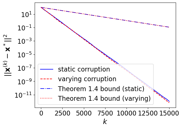
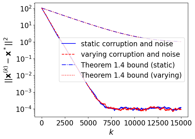
Figure 3. Empirical behavior of QRK ($q=0.6$) and upper bound provided in Theorem 1.4 on (left) static noise-free (${\mathbf{b}}^{(k)}={\mathbf{b}}+{\mathbf{c}}$) and time-varying noise-free (${\mathbf{b}}^{(k)}={\mathbf{b}}+{\mathbf{c}}^{(k)}$) systems and (right) static noisy (${\mathbf{b}}^{(k)}={\mathbf{b}}+{\mathbf{c}}+{\mathbf{n}}$) and time-varying noisy (${\mathbf{b}}^{(k)}={\mathbf{b}}+{\mathbf{c}}^{(k)}+{\mathbf{n}}^{(k)}$) systems defined by $A\in\mathbb{R}^{20000\times 100}$ where corruption vectors are generated with $\beta m$ uniformly randomly selected entries equal to one and the remainder equal to 0 where $\beta=0.001$. The noise vectors have entries sampled i.i.d. from $\mathcal{N}(0,0.001)$.

3.2. QRK on systems with time-varying noise and corruption

In this section we compare the upper bound in Theorem 1.4 to the empirical behavior of QRK on a system with time-varying noise and corruption. We generate a system with $A\in\mathbb{R}^{20000\times 100}$ generated with i.i.d. entries sampled from $\mathcal{N}(0,1)$ and row-normalize $A$, we generate ${\mathbf{x}}^{*}\in\mathbb{R}^{100}$ with i.i.d. entries sampled from $\mathcal{N}(0,1)$, and ${\mathbf{b}}^{(k)}=A{\mathbf{x}}^{*}+{\mathbf{n}}^{(k)}+{\mathbf{c}}^{(k)}$ where in each iteration ${\mathbf{n}}^{(k)}$ is sampled from $\mathcal{N}(0,\sigma^{2})$ and we have corruption vector ${\mathbf{c}}^{(k)}$ defined by $\beta=|\text{supp}({\mathbf{c}}^{(k)})|/m$ with randomly selected entries set to $10$. Finally, we implement QRK on this system with a quantile of size $q$. In Figure 4 we provide a set of three plots illustrating how the empirical behavior of QRK and the bound of Theorem 1.4 vary with respect to $q$, $\beta$, and $\sigma$.

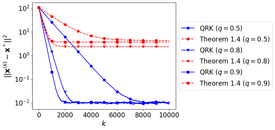
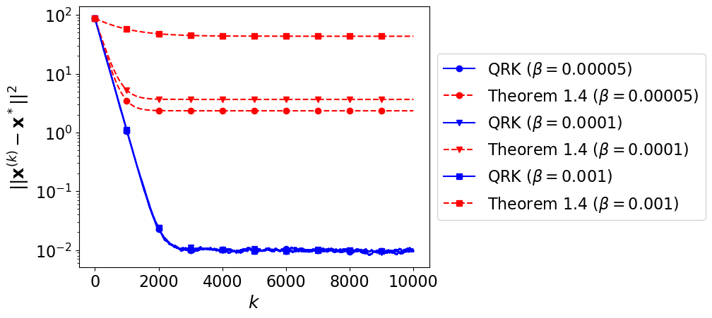
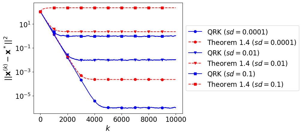
Figure 4. Empirical behavior of QRK and upper bound provided in Theorem 1.4 on system defined by $A\in\mathbb{R}^{20000\times 100}$ and ${\mathbf{b}}^{(k)}={\mathbf{b}}+{\mathbf{n}}^{(k)}+{\mathbf{c}}^{(k)}$ where corruption ${\mathbf{c}}^{(k)}$ is a vector with $\beta m$ uniformly randomly selected entries equal to the corruption size (10) and the remainder equal to 0. The noise ${\mathbf{n}}^{(k)}$ is an i.i.d. random vector sampled in each iteration with entries from $\mathcal{N}(0,\sigma^{2})$. The upper left shows behavior as $q$ varies between 0.5, 0.8 and 0.9, while $\beta=0.00005$ and $\sigma=0.01$. The upper right shows behavior as $\beta$ varies between 0.00005, 0.0001 and 0.001, while $q=0.8$ and $\sigma=0.01$. The lower center shows behavior as $\sigma$ varies between 0.0001, 0.01 and 0.1, while $q=0.8$ and $\beta=0.00005$. Experiments are averaged over 10 trials.

3.3. QRK for corruption detection

In this section, we compare the fraction of corrupted indices that are detected by the largest magnitude entries of the residual of QRK to the lower bound on the probability that all are detected provided by Corollary 1.4.2. We generate a system with $A\in\mathbb{R}^{20000\times 100}$ generated with i.i.d. entries sampled from $\mathcal{N}(0,1)$, then row-normalize $A$, generate ${\mathbf{x}}^{*}\in\mathbb{R}^{100}$ with i.i.d. entries sampled from $\mathcal{N}(0,100)$, and ${\mathbf{b}}^{(k)}=A{\mathbf{x}}^{*}+{\mathbf{c}}^{(k)}$ where in each iteration we have corruption vector ${\mathbf{c}}^{(k)}$ defined by $\beta=|\text{supp}({\mathbf{c}}^{(k)})|/m=0.001$ with randomly selected entries set to $10$. Finally, we implement QRK on this system with a quantile of size $q=0.6$. We plot the fraction of corrupted indices that are included in the largest magnitude $\beta m$ entries of the residuals of the QRK iterates. We also plot the lower bound on the probability that all $\beta m$ corrupted indices are included in the largest magnitude entries of the residuals of the QRK iterates, that is, the probability that these entries are easily detectable. We plot these two values over all 8000 iterations of the QRK trial in Figure 5. We note that the lower bound on the probability provided in Corollary 1.4.2 is a conservative estimate given how quickly the QRK residuals reveal the time-varying corrupted indices. This bound is likely loose due to the looseness of the upper bound on the convergence rate.

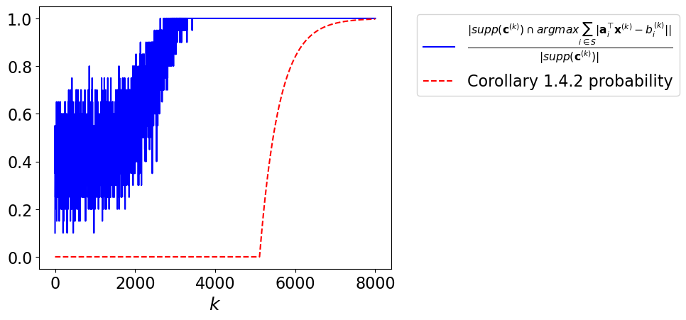
Figure 5. Fraction of corrupted indices in the largest magnitude entries of the QRK ($q=0.6$) iterate residuals and lower bound on probability of detection provided by Corollary 1.4.2 on system defined by $A\in\mathbb{R}^{20000\times 100}$ and ${\mathbf{b}}^{(k)}=A{\mathbf{x}}^{*}+{\mathbf{c}}^{(k)}$ with corruption rate $\beta=0.001$.

3.4. RK on systems with time-varying noise

In this section, we compare the upper bound provided by Theorem 2.1 to the empirical behavior of RK on systems with noise vectors ${\mathbf{n}}^{(k)}$ with entries drawn i.i.d. from a distribution with mean $\mu$ and standard deviation $\sigma$. We generate a system with $A\in\mathbb{R}^{20000\times 100}$ generated with i.i.d. entries sampled from $\mathcal{N}(0,1)$, ${\mathbf{x}}^{*}\in\mathbb{R}^{100}$ with i.i.d. entries sampled from $\mathcal{N}(0,1)$, and ${\mathbf{b}}^{(k)}=A{\mathbf{x}}^{*}+{\mathbf{n}}^{(k)}$ where in each iteration ${\mathbf{n}}^{(k)}$ is sampled from $\mathcal{N}(\mu,\sigma^{2})$ where $\mu\in\{0,0.01,0.1\}$ and $\sigma\in\{0,0.01,0.1\}$ are noted. In Figure 6, we plot the error of the RK method and the upper bounds on this error given in Theorem 2.1 on these systems. We note that these upper bounds are quite tight due to the consistent form of the sampled noise across iterations.

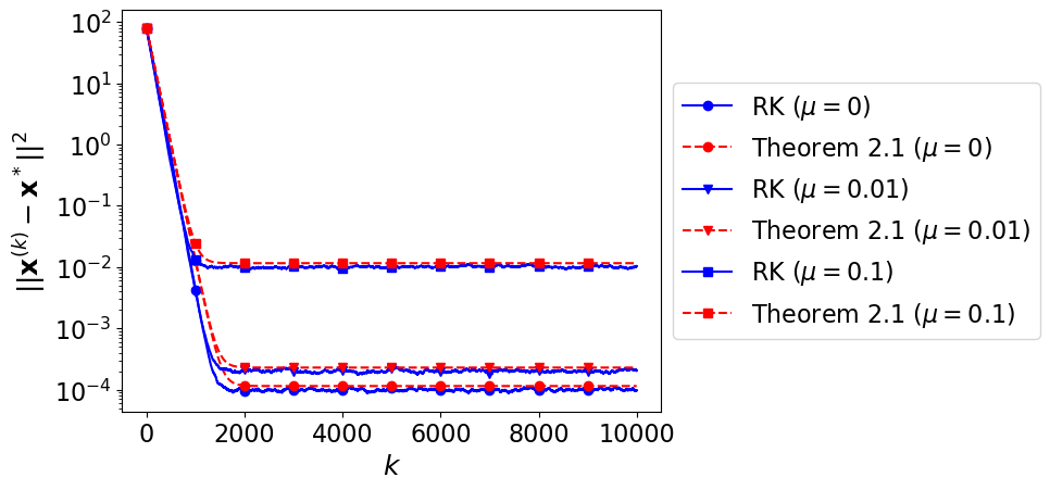
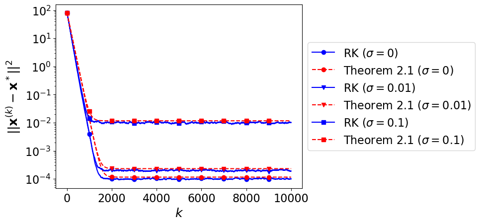
Figure 6. Empirical behavior of RK and upper bound provided in Theorem 2.1 on system defined by $A\in\mathbb{R}^{20000\times 100}$ and ${\mathbf{b}}^{(k)}=A{\mathbf{x}}^{*}+{\mathbf{n}}^{(k)}$ where noise ${\mathbf{n}}^{(k)}$ is an i.i.d. random vector sampled in each iteration with entries from $\mathcal{N}(\mu,\sigma^{2})$. The plot on the left shows behavior as $\mu$ varies between 0, 0.01, and 0.1, while $\sigma=0.01$. The plot on the right shows behavior as $\sigma$ varies between 0, 0.01, and 0.1, while $\mu=0.01$. Experiments are averaged over 10 trials.

4. Conclusion

In this work, we prove that the QRK method converges even in the presence of time-varying perturbation by noise and corruption. We provide an upper bound on the error of the QRK iterates, which includes a convergence horizon term dictated by the magnitude of the time-varying noise and a rate term that depends upon the corruption rate of the time-varying corruption perturbing the system. We specialize this result to several noise models: bounded noise, random noise with given mean and standard deviation, and noise sampled from $\mathcal{N}(0,\sigma^{2})$. We additionally use these results to provide a lower bound on the probability that the corrupted indices will be revealed by examining the QRK iterate residuals.

Our numerical experiments illustrate our theoretical results and reveal that many of our estimates are conservative. These results reflect the qualitative behavior of the QRK method, but are quite loose, likely due to the looseness of the convergence rate estimate and the convergence horizon bound.

We highlight that our results are tailored to hold for time-varying and potentially adversarial corruption. A very interesting future question, given by Steinerberger [39], is whether QRK can be shown to converge for a larger fraction of corruptions, say near 50%, when the corrupted indices are chosen at random. This corruption model seems very reasonable for a distributed computing application where corruption could occur during data access.

Another interesting future question is to develop a variant of RK that is robust to corruption and noise simultaneously, breaking the convergence horizon suffered by QRK in the presence of noise. In the corruption-free case, the Randomized Extended Kaczmarz (REK) method [45] utilizes a column-wise projection step, in addition to the usual RK projections, to break the convergence horizon and converge to the least-squares solution. Providing such a method which is simultaneously robust to corruption would be a useful contribution.

References

• [1] D. Alistarh, Z. Allen-Zhu, and J. Li. Byzantine stochastic gradient descent. Advances in Neural Information Processing Systems, 31, 2018.
• [2] P. Awasthi, M. F. Balcan, and P. M. Long. The power of localization for efficiently learning linear separators with noise. In Proceedings of the forty-sixth annual ACM symposium on Theory of computing, pages 449–458, 2014.
• [3] K. Bhatia, P. Jain, P. Kamalaruban, and P. Kar. Consistent robust regression. In I. Guyon, U. V. Luxburg, S. Bengio, H. Wallach, R. Fergus, S. Vishwanathan, and R. Garnett, editors, Advances in Neural Information Processing Systems, volume 30. Curran Associates, Inc., 2017.
• [4] P. Blanchard, E. M. El Mhamdi, R. Guerraoui, and J. Stainer. Machine learning with adversaries: Byzantine tolerant gradient descent. Advances in neural information processing systems, 30, 2017.
• [5] S. Boyd and L. Vandenberghe. Convex optimization. Cambridge university press, 2004.
• [6] M. Charikar, J. Steinhardt, and G. Valiant. Learning from untrusted data. In Proceedings of the 49th Annual ACM SIGACT Symposium on Theory of Computing, pages 47–60, 2017.
• [7] X. Chen and A. Powell. Almost sure convergence of the Kaczmarz algorithm with random measurements. J. Fourier Anal. Appl., pages 1–20, 2012. 10.1007/s00041-012-9237-2.
• [8] L. Cheng, B. Jarman, D. Needell, and E. Rebrova. On block accelerations of quantile randomized kaczmarz for corrupted systems of linear equations. Inverse Problems, 2022. To appear.
• [9] I. Diakonikolas, G. Kamath, D. Kane, J. Li, A. Moitra, and A. Stewart. Robust estimators in high-dimensions without the computational intractability. SIAM Journal on Computing, 48(2):742–864, 2019.
• [10] I. Diakonikolas, G. Kamath, D. Kane, J. Li, J. Steinhardt, and A. Stewart. Sever: A robust meta-algorithm for stochastic optimization. In International Conference on Machine Learning, pages 1596–1606. PMLR, 2019.
• [11] B. Dumitrescu. On the relation between the randomized extended Kaczmarz algorithm and coordinate descent. BIT, pages 1–11, 2014.
• [12] Y. C. Eldar and D. Needell. Acceleration of randomized Kaczmarz method via the Johnson-Lindenstrauss lemma. Numer. Algorithms, 58(2):163–177, 2011.
• [13] R. Gordon, R. Bender, and G. T. Herman. Algebraic reconstruction techniques (ART) for three-dimensional electron microscopy and X-ray photography. J. Theoret. Biol., 29:471–481, 1970.
• [14] J. Haddock, A. Ma, and E. Rebrova. On subsampled quantile randomized Kaczmarz. In Proc. Allerton Conf. on Communication, Control, and Computing, 2023.
• [15] J. Haddock, D. Needell, E. Rebrova, and W. Swartworth. Quantile-based iterative methods for corrupted systems of linear equations. SIAM Journal on Matrix Analysis and Applications, 43(2):605–637, 2022.
• [16] G. Herman and L. Meyer. Algebraic reconstruction techniques can be made computationally efficient. IEEE T. Med. Imaging, 12(3):600–609, 1993.
• [17] B. Jarman and D. Needell. QuantileRK: Solving large-scale linear systems with corrupted, noisy data. 2021.
• [18] S. Kaczmarz. Angenäherte auflösung von systemen linearer gleichungen. Bull. Int. Acad. Polon. Sci. Lett. Ser. A, pages 335–357, 1937.
• [19] K. A. Lai, A. B. Rao, and S. Vempala. Agnostic estimation of mean and covariance. In 2016 IEEE 57th Annual Symposium on Foundations of Computer Science (FOCS), pages 665–674. IEEE, 2016.
• [20] F. C. Leone, L. S. Nelson, and R. Nottingham. The folded normal distribution. Technometrics, 3(4):543–550, 1961.
• [21] X. Li, L. Huang, and D. Needell. Distributed randomized kaczmarz for the adversarial workers. arXiv preprint arXiv:2203.00095, 2022.
• [22] J. Liu, S. J. Wright, and S. Sridhar. An asynchronous parallel randomized Kaczmarz algorithm. arXiv preprint arXiv:1401.4780, 2014.
• [23] A. Ma, D. Needell, and A. Ramdas. Convergence properties of the randomized extended Gauss–Seidel and Kaczmarz methods. SIAM J. Matrix Anal. A., 36(4):1590–1604, 2015.
• [24] N. F. Marshall and O. Mickelin. An optimal scheduled learning rate for a randomized kaczmarz algorithm. SIAM Journal on Matrix Analysis and Applications, 44(1):312–330, 2023.
• [25] J. D. Moorman, T. K. Tu, D. Molitor, and D. Needell. Randomized Kaczmarz with averaging. BIT, pages 1–23, 2020.
• [26] M. S. Morshed, M. S. Islam, and M. Noor-E-Alam. Accelerated sampling Kaczmarz Motzkin algorithm for the linear feasibility problem. J. Global Optim., pages 1–22, 2019.
• [27] D. Needell. Randomized Kaczmarz solver for noisy linear systems. BIT, 50(2):395–403, 2010.
• [28] D. Needell, N. Srebro, and R. Ward. Stochastic gradient descent and the randomized Kaczmarz algorithm. Math. Program. A, 155(1):549–573, 2016.
• [29] D. Needell and J. A. Tropp. Paved with good intentions: Analysis of a randomized block Kaczmarz method. Linear Algebra Appl., 2013.
• [30] C. Popa. A fast Kaczmarz-Kovarik algorithm for consistent least-squares problems. Korean J. Comput. Appl. Math., 8(1):9–26, 2001.
• [31] C. Popa. A Kaczmarz-Kovarik algorithm for symmetric ill-conditioned matrices. An. Ştiinţ. Univ. Ovidius Constanţa Ser. Mat., 12(2):135–146, 2004.
• [32] C. Popa, T. Preclik, H. Köstler, and U. Rüde. On Kaczmarz’s projection iteration as a direct solver for linear least squares problems. Linear Algebra Appl., 436(2):389–404, 2012.
• [33] A. Prasad, A. S. Suggala, S. Balakrishnan, P. Ravikumar, et al. Robust estimation via robust gradient estimation. Journal of the Royal Statistical Society Series B, 82(3):601–627, 2020.
• [34] H. Robbins and S. Monro. A stochastic approximation method. Ann. Math. Statist., 22:400–407, 1951.
• [35] P. J. Rousseeuw. Least median of squares regression. Journal of the American statistical association, 79(388):871–880, 1984.
• [36] Y. Saad. Iterative methods for sparse linear systems. SIAM, 2003.
• [37] A. Savvides, C.-C. Han, and M. B. Strivastava. Dynamic fine-grained localization in ad-hoc networks of sensors. In Proceedings of the 7th annual international conference on Mobile computing and networking, pages 166–179, 2001.
• [38] V. Shah, X. Wu, and S. Sanghavi. Choosing the sample with lowest loss makes SGD robust. In S. Chiappa and R. Calandra, editors, Proceedings of the Twenty Third International Conference on Artificial Intelligence and Statistics, volume 108 of Proceedings of Machine Learning Research, pages 2120–2130. PMLR, 26–28 Aug 2020.
• [39] S. Steinerberger. Quantile-based random Kaczmarz for corrupted linear systems of equations. Information and Inference: A Journal of the IMA, 12(1):448–465, 2023.
• [40] T. Strohmer and R. Vershynin. A randomized Kaczmarz algorithm with exponential convergence. J. Fourier Anal. Appl., 15(2):262–278, 2009.
• [41] T. Strohmer and R. Vershynin. A randomized Kaczmarz algorithm with exponential convergence. Journal of Fourier Analysis and Applications, 15(2):262, 2009.
• [42] L. Tondji, I. Tondji, and D. A. Lorenz. Adaptive bregman-kaczmarz: An approach to solve linear inverse problems with independent noise exactly. arXiv preprint arXiv:2309.06186, 2023.
• [43] J. Á. Víšek. The least trimmed squares. Part I: Consistency. Kybernetika, 42(1):1–36, 2006.
• [44] A. Zouzias and N. M. Freris. Randomized extended Kaczmarz for solving least squares. SIAM J. Matrix Anal. A., 34(2):773–793, 2013.
• [45] A. Zouzias and N. M. Freris. Randomized gossip algorithms for solving Laplacian systems. In 2015 European Control Conference (ECC), pages 1920–1925. IEEE, 2015.