A generalized approach for rapid entropy calculation of liquids and solids

Abstract

We build a comprehensive methodology for the fast computation of entropy across both solid and liquid phases. The proposed method utilizes a single trajectory of molecular dynamics (MD) to facilitate the calculation of entropy, which is composed of three components. The electronic entropy is determined through the temporal average acquired from density functional theory (DFT) MD simulations. The vibrational entropy, typically the predominant contributor to the total entropy, even within the liquid state, is evaluated by computing the phonon density of states via the velocity auto-correlation function. The most arduous component to quantify, the configurational entropy, is assessed by probability analysis of the local structural arrangement and atomic distribution. We illustrate, through a variety of examples, that this method is both a versatile and valid technique for characterizing the thermodynamic states of both solids and liquids. Furthermore, this method is employed to expedite the calculation of melting temperatures, demonstrating its practical utility in computational thermodynamics.

Entropy is a fundamental concept in thermodynamics, representing the degree of disorder or randomness in a system. While crucial, accurately computing entropy is challenging due to its non-intuitive nature and the complexity of accounting for the microstates of a system. This computational difficulty underscores the intricacies of predicting system behavior where energy distribution and disorder are intricate variables.

Recent advancements in the calculation of entropy have significantly enhanced our understanding of microstate analysis and energy distribution. These sophisticated methodologies, while providing comprehensive insights into the fundamental aspects of entropy, introduce specific computational challenges and are confined to a narrow application spectrum. The Particle Insertion Method Widom (1963, 1982) relies on probabilistic evaluations, deeply intertwined with statistical mechanics principles and chemical potential. Despite its efficacy Hong and van de Walle (2012), it demands significant computational investment, relying on a large amount of insertion trials to achieve statistically significant results, rendering it extremely expensive when integrated with DFT Hong and van de Walle (2012). The Pair Distribution Function method Green (1952); Wallace (1987); Widom and Gao (2019) analyzes spatial particle correlations against an ideal gas benchmark, translating these into entropy metrics. The method, however, relies on an expansion of entropy in multiparticle correlations beyond the pair-entropy term, potentially increasing complexity and resulting in truncation errors and large fluctuations. Lastly, the Two-Phase Thermodynamics Method Lin et al. (2003) presents a creative approach by conceiving the system as a combination of solid-like and gas-like phases. This method uniquely separates solid-state phonon contributions, which possess a well-defined analytical entropy expression, and approximates the remainder of the system as a gas phase, e.g., modeled using hard spheres. The efficacy and accuracy of this method are contingent upon the artificial division into solid-like and gas-like components and the specific selection of the gas-like phase model.

In the present study, we introduce a comprehensive methodology designed to generalize the computation of entropy in both solid and liquid states, especially for high temperature applications, enabling us to calculate entropy from one DFT MD trajectory. The method adopts recent advancements in the field, including the concepts of entropy “coarse-graining” van de Walle and Ceder (2002) and the Zentropy theory Liu et al. (2022), which further segment entropy into distinct categories - configurational, vibrational, and electronic, aiming to encapsulate entropy at various levels, acknowledging its multi-layered nature. (There is no rotational entropy for bulk solids or liquids, as it is part of the vibrational entropy.)

$$S=S_{\text{conf}}+S_{\text{vib}}+S_{\text{elec}}.$$ (1)

These theoretical frameworks offer a granular understanding of free energy and entropy, enabling feasible computation and a more detailed analysis of thermodynamic properties. Furthermore, incorporating $S_{\text{vib}}$ (based on phonon analysis under the harmonic approximation at high temperature) and $S_{\text{elec}}$ (based on quantum mechanical calculation of electronic density of states) allows the assimilation of quantum mechanical effects, such as quantum harmonic oscillation of phonons and the Fermi-Dirac distribution of electrons, thereby facilitating a quantum thermodynamic description that reconciles with classical mechanics at sufficiently high temperatures.

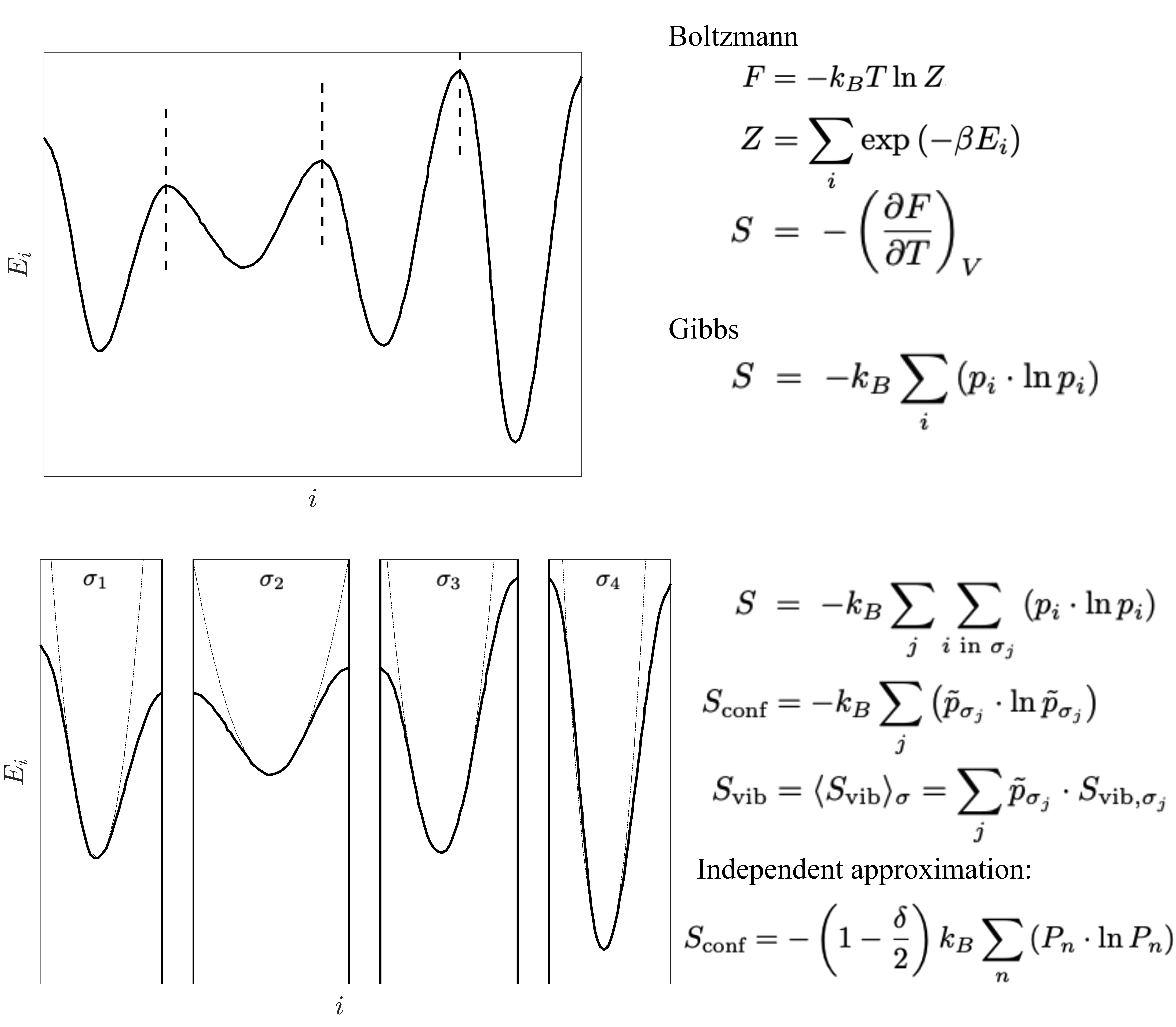
Figure 1: Diagram for segmentation of entropy into configurational and vibrational terms.

Here we outline a theory underpinning our methodology, with comprehensive derivations detailed in the Supplemental Material. This theory is anchored in the seminal interpretations of entropy by Boltzmann Perrot (1998) and Gibbs et al. Gibbs (1960); von Neumann (1927); Shannon (1948), which are demonstrated to be equivalent (see Supplemental Material), thus allowing for their interchangeable application. As shown in Fig. 1, we write the combined configurational and vibrational entropy ($S_{\text{conf}}+S_{\text{vib}}$) employing Gibbs’s formula,

$$S=-k_{B}\sum_{i}{\left(p_{i}\cdot\ln{p_{i}}\right)},$$ (2)

where $p_{i}$ denotes the probability of microstate $i$ within the coordinate space $\mathbb{R}$. Proceeding to segment the space into configurations $\sigma$, we separate $S_{\text{conf}}$ and $S_{\text{vib}}$, as detailed in the Supplemental Material,

$$S_{\text{conf}} = -k_{B}\sum_{j}{\left(\tilde{p}_{\sigma_{j}}\cdot\ln{\tilde{p}_{\sigma_{j}}}\right)},$$ (3)

$$S_{\text{vib}} = \langle S_{\text{vib}}\rangle_{\sigma}=\sum_{j}{\tilde{p}_{\sigma_{j}}\cdot S_{\text{vib},\sigma_{j}}},$$ (4)

where $\tilde{p}_{\sigma_{j}}$ is the aggregated $p_{i}$ within configuration $\sigma_{j}$ and thus the configuration’s probability. We prove in the Supplemental Material that, under an assumption of atomic probability independence, Eqn. 3 can be simplified, allowing the substitution of the configuration probability $\tilde{p}_{\sigma}$ with atomic local probability $P_{n}$,

$$S_{\text{conf}}=-\left(1-\frac{\delta}{2}\right)k_{B}\sum_{n}{\left(P_{n}\cdot\ln{P_{n}}\right)},$$ (5)

where $P_{n}$ stands for the overall probability of an atom having $n$ nearest neighbors, and $\delta$ is assigned a value of 1 if the pair consists of the same element, and 0 otherwise. For detailed derivations of Eqns. 2 through 5, readers are directed to the Supplemental Material.

Utilizing Eqns. 5 and 4, we are now able to compute $S_{\text{conf}}$ and $S_{\text{vib}}$ from a single MD trajectory. The configurational entropy, previously a formidable task, now can be evaluated from the atomic local probability $P_{n}$, the probability of occurrence of a local structural arrangement. To implement this, we perform a pairwise radial distribution function analysis to determine the nearest neighbor cutoff radius. Subsequently, we count the nearest neighbors located within this radial boundary. The resultant probability $P_{n}$ is then applied in Eqn. 5 to compute the configurational entropy, as shown in Fig. 2.

Concurrently, the vibrational entropy $S_{\text{vib}}$ is deduced from the same MD trajectory. According to Eqn. 4, the overall vibrational entropy is the ensemble average of all configurations $\sigma$, attainable through MD’s effective configuration sampling, given a sufficiently high diffusion rate. This characteristic is typically observed in liquids or disordered solid states with light elements at high temperatures, where the dynamic nature of the system promotes rapid exploration of configurational space. In this analysis, we pivot to Boltzmann’s entropy interpretation within the harmonic approximation (also see the Supplemental Material),

$$F=k_{B}T\int{\ln{\left[2\sinh(\frac{h\nu}{2k_{B}T})\right]}g(\nu)d\nu},$$ (6)

where $\nu$ is phonon frequency and $g(\nu)$ is phonon density of states (DoS). To implement it, the phonon DoS is calculated from velocity auto-correlation of the MD trajectory, as detailed in the Supplemental Material and the works by Frenkel Frenkel and Smit (2001) and Goddard Lin et al. (2003).

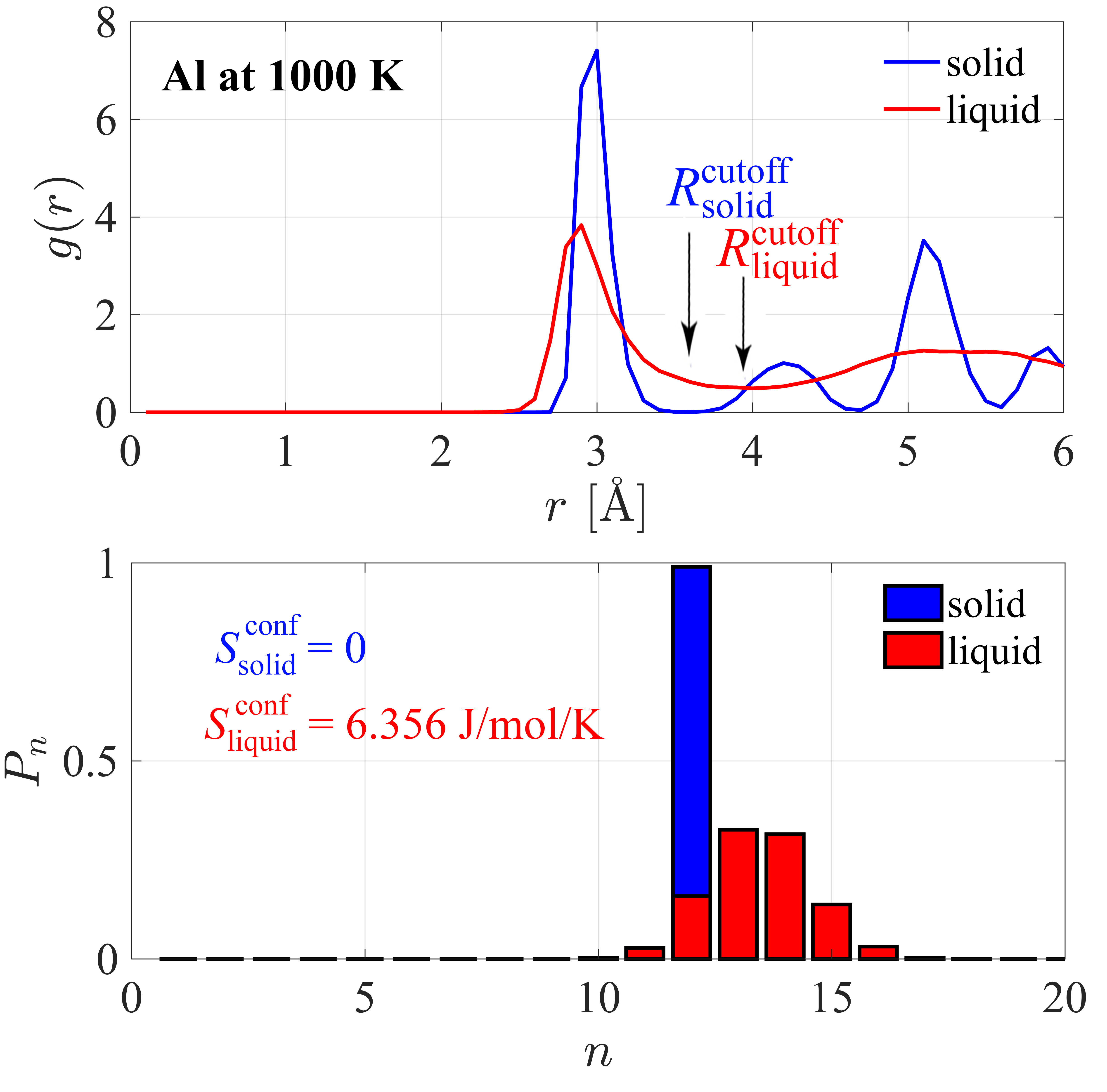
Figure 2: Radial distribution function (upper) and probability $P_{n}$ of local configurations of solid (fcc) and liquid aluminum at 1000 K.

The electronic entropy, the last term in Eqn. 1, is computed by averaging electronic entropy values of electronic structures obtained during the DFT-based MD trajectory. While our analysis presumes either diamagnetic or paramagnetic characteristics for the sake of simplicity, the underlying theoretical framework is sufficiently versatile to accommodate the examination of configurations influenced by magnetic spin orientations.

The methodology presented herein exhibits four distinct advantages. First, it enables the direct computation of entropy from a singular MD trajectory, markedly simplifying the entropy calculation process. Second, it properly partitions coordinate space to configurational $S_{\text{conf}}$ and vibrational $S_{\text{vib}}$ components, followed by a summation of all states. This partitioning and summation are designed to (1) include all states significant to the system’s entropy without missing any meaningful piece, and (2) preclude the possibility of state double-counting. These requirements had been the major challenge for direct entropy calculation, e.g., it is difficult to know the number of configurations in a liquid. Third, the method ensures a highly accurate description of the vibrational entropy, often the predominant entropy term (see Fig. 3). This accuracy is achieved through the evaluation of phonon DoS from velocity auto-correlation, an avenue that inherently accounts for quantum effects, thus offering an advantage over classical mechanics methods such as particle insertion or pairwise distribution analysis. While still under the harmonic approximation, the frequencies are derived from MD movements within the high-temperature region of the potential energy surface, thereby incorporating some degree of anharmonic effects. This approach contrasts with Hessian matrix calculation from atomic displacements, which is generally conducted at the bottom of the potential well. Finally, the proposed method demonstrates its versatility by generalizing across both solid and liquid states. This includes a wide spectrum of materials, ranging from defect-free ordered solids and partially disordered solids with defects to lattice-free liquids. As elucidated in the subsequent sections, this breadth underscores the method’s applicability to a broad array of material phases and conditions.

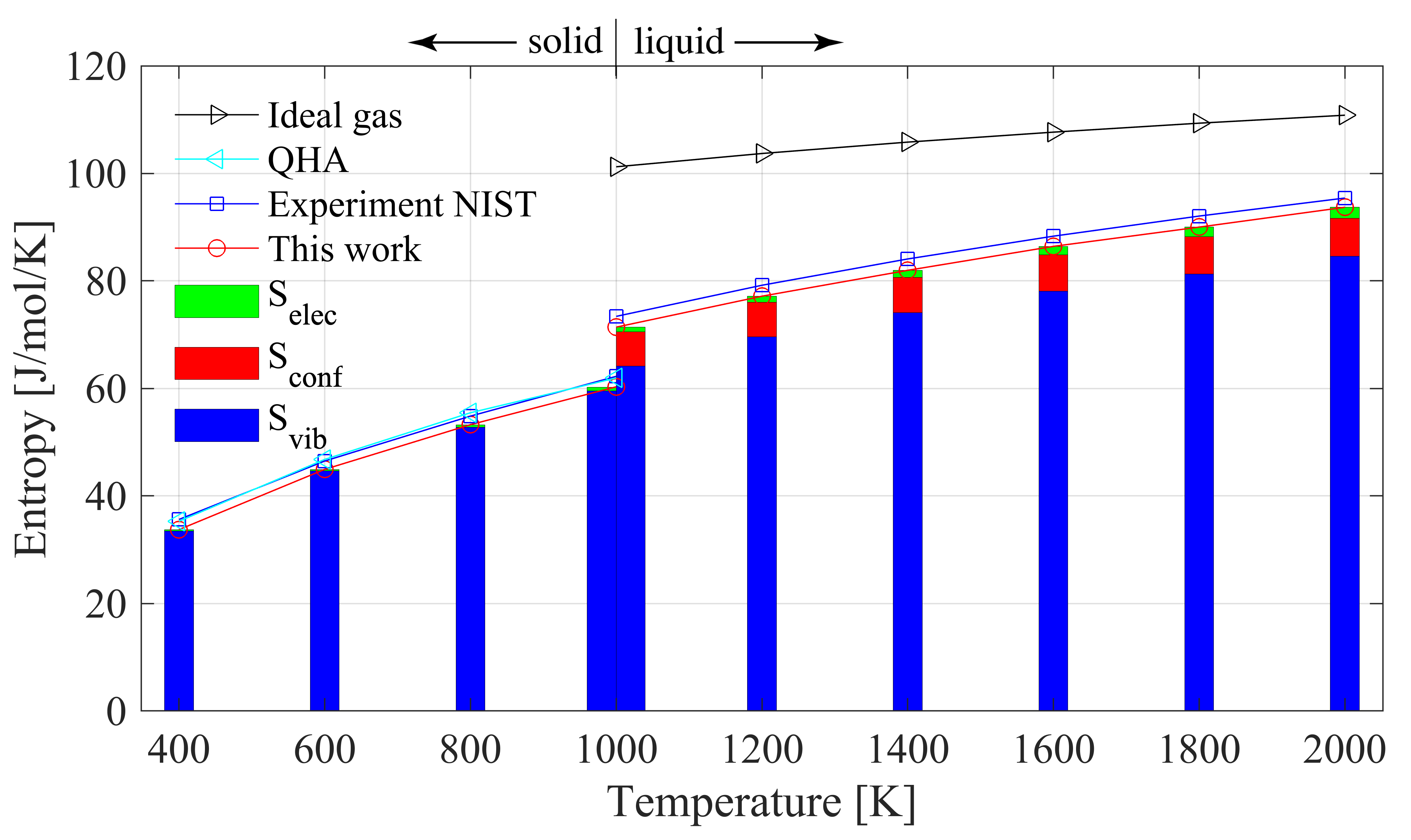
Figure 3: Entropy and its configurational, vibrational, and electronic components at various temperatures for solid (400-1000 K) and liquid (1000-2000 K) phases of aluminum.

Table 1: Thermodynamic properties and transition dynamics of materials

Material	Phase	$T$ [K]	$S$ [J/K/mol atom]					$H$	$\Delta H$	$\Delta S$	$T$	$T_{\text{exp}}$	$T_{\text{DFT}}$b
		MD	Vib.	Conf.	Elec.	Total	Expt.a	[eV/atom]	[J/mol at.]	[J/K/mol at.]	[K]	[K]	[K]
Al	fcc	1000	59.038	0.017	0.699	59.754	62.25c	-3.604	fcc $\rightarrow$ liquid
Al	liquid	1000	63.807	6.339	0.870	71.016	73.40	-3.502	9850	11.262	875	933	999
Ti	bcc	1800	79.451	2.369	7.189	89.009	87.47	-7.435	bcc $\rightarrow$ liquid
Ti	liquid	1800	81.461	6.424	7.050	94.935	94.42c	-7.336	10274	5.926	1734	1957	1952
Si	diamond	1400	57.604	0.000	0.178	57.781	56.46	-5.218	diamond $\rightarrow$ liquid
Si	liquid	1400	74.830	6.955	1.414	83.200	87.12c	-4.795	40767	25.418	1604	1687	1785
W	bcc	3400	99.171	0.179	6.409	105.759	104.3	-12.241	bcc $\rightarrow$ liquid
W	liquid	3400	105.994	6.230	7.710	119.934	115.7c	-11.778	44745	14.175	3157	3685	3470
Fe	bcc	1500	66.912	3.274	6.600	76.786	84.52	-7.790	bcc $\rightarrow$ liquid
Fe	liquid	1500	70.428	6.167	7.167	83.762	92.9c	-7.657	12778	6.976	1832	1784	1828
Fe	fcc	1500	66.273	1.164	6.475	73.912	84.42	-7.834	fcc (metastable)$\rightarrow$liquid
Fe	liquid	1500	70.428	6.167	7.167	83.762	92.9c	-7.657	17094	9.850	1735	-	-
Fe, 100GPa	hcp	3500	77.627	0.947	11.158	89.732	-	-1.729	At 100GPa: hcp$\rightarrow$liquid
Fe, 100GPa	liquid	3500	81.571	6.039	12.003	99.613	-	-1.369	34726	9.881	3514	3787	4019
ZrO2	fluorite	2800	76.739	4.402	0.225	81.365	71.6	-9.053	fluorite $\rightarrow$ liquid
ZrO2	liquid	2800	77.739	8.118	0.285	86.142	81.3c	-8.907	14095	4.776	2951	2973	-
HfO2	fluorite	3000	76.704	4.311	0.151	81.165	-	-9.655	fluorite $\rightarrow$ liquid
HfO2	liquid	3000	78.369	7.791	0.252	86.412	-	-9.494	15577	5.246	2969	3053	3313
Er2O3	H phase	2900	82.413	4.455	0.209	87.077	-	-7.841	H phase $\rightarrow$ liquid
Er2O3	liquid	2900	83.065	6.677	0.260	90.001	-	-7.751	8786	2.924	3005	2693d	2752
HfC0.5N0.38	rocksalt	4000	87.774	3.223	3.344	94.341	-	-9.982	rocksalt $\rightarrow$ liquid
HfC0.5N0.38	liquid	4000	97.671	8.625	5.568	111.864	-	-9.139	81333	17.523	4641	-	4141
HfC0.88	rocksalt	4000	87.764	2.890	3.595	94.249	-	-9.726	rocksalt $\rightarrow$ liquid
HfC0.88	liquid	4000	97.791	8.717	5.818	112.327	-	-8.904	79235	18.078	4383	-	3898
HfC	rocksalt	4000	86.173	2.219	3.046	91.438	-	-9.719	rocksalt $\rightarrow$ liquid
HfC	liquid	4000	96.912	9.001	5.508	111.422	-	-8.859	83013	19.984	4154	4223	3842

DFT calculations were performed by the Vienna Ab initio Simulation Package (VASP) Kresse and Joubert (1999), with the projector-augmented-wave (PAW) Blöchl (1994) implementation and the generalized gradient approximation (GGA) for exchange correlation energy, in the form known as Perdew, Burke, and Ernzerhof (PBE) Perdew et al. (1996). The electronic temperature is accounted for by imposing a Fermi distribution of the electrons on the energy level density of states, so it is consistent with the ionic temperature. For all materials, the planewave energy cutoff is set to the default value (normal precision) of the pseudopotential during the MD simulations, and it is further increased to the high-precision value during the correction for the Pulay stress Francis and Payne (1990). DFT MD techniques are utilized to simulate atomic movements and trajectories. Specifically, MD simulations are carried out under constant number of atoms, pressure and temperature condition ($NPT$, isothermal-isobaric ensemble). Here the thermostat is conducted under the Nosé-Hoover chain formalism Nosé (1984a, b); Hoover (1985); Martyna and Klein (1992). The barostat is realized by adjusting volume every 80 steps according to average pressure, implemented in our SLUSCHI (Solid and Liquid in Ultra Small Coexistence with Hovering Interfaces) package Hong and van de Walle (2016). Although this does not formally generate an isobaric ensemble, this approach has been shown to provide an effective way to change volume smoothly and to avoid the unphysical large oscillation caused by commonly used barostats in small cells Hong and van de Walle (2013).

As our first example, we calculate the entropy of solid and liquid phase aluminum, comparing these findings with experimental data across a temperature range of 400 to 2000 K. Given aluminum’s simple metallic nature and the high accuracy afforded by DFT, it exemplifies an ideal candidate for validating the efficacy of this approach. Such comparative analysis offers compelling validation for the precision of this new approach.

As shown in Fig. 3, the new method exhibits remarkable accuracy in estimating the entropy of aluminum in both its solid and liquid states, with discrepancies limited to 3 J/mol/K. Further scrutiny into the entropy components reveals the method’s significant advantages: the predominant contribution of vibrational entropy, compared with the considerably lesser role of configurational entropy, which is much smaller by an order of magnitude in liquids and is negligible in solids. This underscores the imperative of accurately quantifying vibrational entropy in thermodynamic assessments. By fundamentally prioritizing vibrational and phonon considerations, this new approach demonstrates a distinct superiority in capturing the intricate dynamics of entropy.

The success on both fcc Al, a defect-free solid with zero configurational entropy, and its liquid state, a lattice-free disordered phase with significantly higher configurational entropy, demonstrates the capability of this generalized approach in not only entropy calculations but also the determination of phase boundaries. Based on entropies calculated by this method and enthalpies from the same DFT MD trajectories, as shown in Table 1, we are able to calculate the melting temperature of Al. The value of 875 K is in close agreement with the experimental melting temperature of 933 K.

The observed discrepancy, as illustrated in Figure 3, can be attributed to the omission of long-wavelength phonons, a consequence of the finite dimensions of the simulation cell. This limitation results in an underrepresentation of these phonons, impacting the accuracy of our findings. To mitigate this source of error, two approaches are viable: expanding the size of the system under study, which would naturally incorporate a broader spectrum of phonon wavelengths, or applying a quadratic fit to the phonon density of states (DoS) curve in the low-frequency domain. The latter is predicated on the established principle that long-wavelength phonons exhibit behavior that can be closely approximated by quadratic fitting, offering a method to refine our model’s precision in the future.

As our second example, we investigate zirconium oxide (ZrO₂), a material notable for its polymorphism and high-temperature stability Garvie et al. (1975); Fabrichnaya et al. (2007). ZrO₂ undergoes a phase transformation to the fluorite structure at high temperatures before melting, which is characterized by a significant oxygen ion mobility Kilo et al. (2003); Wang et al. (2006), due to oxygen sublattice melting. This property makes it an excellent candidate for applications as a fast ion conductor. However, the dynamic and partially disordered nature of oxygen diffusion at high temperatures presents a computational challenge for accurately determining the configurational entropy of the fluorite phase, as it assumes a non-zero value reflecting the multitude of attainable configurations.

Our methodology addresses this complexity by enabling the calculation of both vibrational and configurational entropy components, thereby facilitating a comprehensive thermodynamic analysis of ZrO₂ in its high-temperature fluorite phase. As shown in Table 1, the significant configurational entropy associated with oxygen (O: 6.574; Zr: 0.057 J/K/mol) underscores the fluidic nature of its sublattice, while zirconium atoms maintain their order. Combined with a calculation on liquid phase of ZrO₂, we determine the melting temperature at 2951 K, compared to the experimental value of 2973 K, and calculate the entropy of fusion to be 14.3 J/K/mol. This calculated fusion entropy, while seemingly lower than the NIST nis (2024) reported value of 29 J/K/mol (which is derived from a linear extrapolation under a constant heat capacity assumption), is in fact more accurate. Contrary to the NIST extrapolation, our recent experimental and computational investigation of ZrO₂ yields an entropy of fusion of 17-18 J/K/mol Hong et al. (2018), showcasing a reasonable agreement with the findings in the present work.

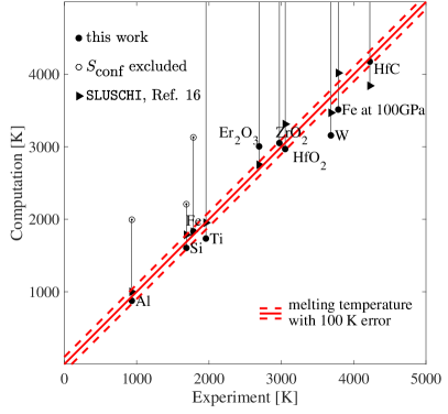
Figure 4: Computational transition temperature based on this method versus experiments. Error bars of 100 K were plotted as red dash lines for eye guide. Plotted are melting temperature of materials at ambient pressure with the GGA-PBE functional employed unless elaborated in the label. Computational details can be found in the Supplemental Material.

As our third example, we delve into hafnium carbonitride, the material we had previously identified Hong and van de Walle (2015) through DFT to surpass HfC and TaC and thereby set a new record for the highest melting temperature, prompting the synthesis and experimental investigation of the carbonitride materials systems Xie et al. (2023); Wyatt et al. (2023). The computational prediction was later corroborated by experimental findings Buinevich et al. (2020). Our new methodology now enables a comprehensive examination that extends to encompass melting temperature, fusion enthalpy, and critically, the entropy of this refractory material. Given the formula $T_{m}=\Delta H/\Delta S$, targeting materials with high fusion enthalpy or low fusion entropy emerges as a strategy for designing high melting temperatures. As revealed in Table 1, the exceptionally large heat of fusion is a major contributing factor for the high melting temperature of the Hf-C and Hf-C-N systems, with 0.84 eV/atom for HfC_0.5N_0.38 compared to 0.82 for HfC_0.88 and 0.86 for HfC. However, an increase in fusion enthalpy alone does not justify the highest melting temperature of hafnium carbonitride: transitioning from HfC_0.88 to HfC_0.5N_0.38 yields only a 2.6% increase in fusion enthalpy, whereas HfC exhibits the highest $\Delta H$ among them. Instead, our findings demonstrated that hafnium carbonitride derives thermodynamic stability from a significantly higher configurational entropy, primarily owing to vacancies and C/N disordering within its solid-state structure, with $\Delta S_{\textrm{conf}}=5.40$ J/K/mol atom for HfC_0.5N_0.38 versus 5.83 for HfC_0.88 and 6.78 for HfC. Notably, these vacancies increase the configurational entropy of the solids, on the C/N sublattice, but not the liquids due to their absence of a lattice structure. The advancement in our methodology allows for the precise quantification of such effects, improving our understanding of the material’s thermodynamic stability.

As our last example, we leverage the developed method to calculate melting temperatures, an important material property that necessitates extensive spatial sampling and thereby incurs significant computational costs Hong (2015). Various materials are investigated, and the results are summarized in Fig. 4. This method demonstrates a high degree of accuracy, generally within a 100 K margin. This level of precision substantially affirms the reliability and effectiveness of our approach in computing entropy, applicable across various states of matter, including liquids, ordered solids, and solids exhibiting degrees of disorder.

The method presented exhibits certain limitations, particularly in its reliance on DFT MD simulations, which are constrained to exploring temporal spans of at most 100 picoseconds. This temporal limitation significantly restricts the diffusion of heavier atoms within ordered lattice structures. This limitation can be resolved in the future with atomic swapping under Metropolis Monte Carlo Metropolis et al. (1953). Additionally, the methodology’s requirement for a clear segregation between configurational and vibrational entropy imposes constraints on the analysis. Specifically, it necessitates that vibrational states associated with adjacent configurations must be distinctly separate to preclude any potential for double counting. This aspect becomes particularly challenging in systems such as body-centered cubic titanium Petry et al. (1991); Kadkhodaei et al. (2017), where the vibrational states of neighboring configurations inherently overlap, complicating the accurate partitioning of entropy contributions.

To summarize, we build a comprehensive methodology for the fast computation of entropy across both solid and liquid phases. The proposed method utilizes a single trajectory of MD to facilitate the calculation of entropy, including electronic, vibrational, and configurational entropies. We propose to calculate the configurational entropy, the most arduous component, as information entropy of nearest neighbors. We illustrate, through a variety of examples, that this method is both a versatile and valid technique for characterizing the thermodynamic states of both solids and liquids. Furthermore, this method is employed to expedite the calculation of melting temperatures, demonstrating its practical utility in computational thermodynamics. The method is implemented in our SLUSCHI package Hong and van de Walle (2016) under the command mds (MD entropy).

I Supplemental Material

I.1 Boltzmann entropy vs. Gibbs entropy

I.1.1 Boltzmann entropy

According to Boltzmann’s statistical interpretation, the Helmholtz free energy is

$$F=-k_{B}T\ln{Z},$$ (S1)

where $Z$ is the partition function, a sum over all microstates $i$,

$$Z=\sum_{i}{\exp{\left(-\beta E_{i}\right)}},$$ (S2)

and

$$\beta=\frac{1}{k_{B}T}.$$ (S3)

The differential form of Helmholtz free energy is

$$dF=-pdV-SdT.$$ (S4)

Thus,

$$S=-\left(\frac{\partial F}{\partial T}\right)_{V}$$ (S5)

Combine Eqns. S1 and S5,

$$S = k_{B}\ln{Z}+k_{B}T\cdot\frac{\sum_{i}{\left(\exp{\left(-\beta E_{i}\right)}\cdot E_{i}\cdot\frac{1}{k_{B}T^{2}}\right)}}{Z}$$ (S6)

$$= k_{B}\ln{Z}+\frac{\sum_{i}{p_{i}E_{i}}}{T}=\frac{-F+\langle E\rangle}{T},$$

where $p_{i}$ is the probability of microstate $i$,

$$p_{i}=\frac{\exp{\left(-\beta E_{i}\right)}}{Z},$$ (S7)

and the probabilities $p_{i}$ is normalized

$$\sum_{i}{p_{i}}=1.$$ (S8)

I.1.2 Gibbs entropy

Gibbs generalized the interpretation of entropy as

$$S=-k_{B}\sum_{i}{\left(p_{i}\cdot\ln{p_{i}}\right)}.$$ (S9)

It is straightforward to prove that this entropy $S$ is equivalent to the Boltzmann entropy.

$$S = -k_{B}\sum_{i}{\left(p_{i}\cdot\ln{p_{i}}\right)}$$ (S10)

$$= -k_{B}\sum_{i}{\left(p_{i}\cdot\ln{\left(\frac{\exp{\left(-\beta E_{i}\right)}}{Z}\right)}\right)}$$

$$= -k_{B}\sum_{i}{\left(p_{i}\cdot\left(-\beta E_{i}-\ln{Z}\right)\right)}$$

$$= \frac{\sum_{i}{p_{i}E_{i}}}{T}+k_{B}\ln{Z}.$$

Now it is clear that Eqns S6 (Boltzmann) and S10 (Gibbs) are the same and the Boltzmann and Gibbs equations can be used interchangeably.

I.2 Segmentation of $S_{\text{conf}}$ and $S_{\text{vib}}$

We then perform the segmentaion of $S$ into $S_{\text{conf}}$ and $S_{\text{vib}}$, by grouping a microstate $i$ into the configuration $\sigma_{j}$ it belongs to, as shown in Fig. 1. According to Gibbs entropy,

$$S = -k_{B}\sum_{i}{\left(p_{i}\cdot\ln{p_{i}}\right)}$$ (S11)

$$= -k_{B}\sum_{j}{\sum_{i\textrm{ in }\sigma_{j}}\left(p_{i}\cdot\ln{p_{i}}\right)}$$

$$= -k_{B}\sum_{j}{\sum_{i\textrm{ in }\sigma_{j}}\left(p_{i}\cdot\ln{\left(\tilde{p}_{\sigma_{j}}\cdot\frac{p_{i}}{\tilde{p}_{\sigma_{j}}}\right)}\right)}$$

$$= -k_{B}\sum_{j}{\left(\tilde{p}_{\sigma_{j}}\cdot\ln{\tilde{p}_{\sigma_{j}}}\right)}$$

$$-k_{B}\sum_{j}{\sum_{i\textrm{ in }\sigma_{j}}\left(p_{i}\cdot\ln{\frac{p_{i}}{\tilde{p}_{\sigma_{j}}}}\right)},$$

where $\tilde{p}_{\sigma_{j}}$ is the sum of $p_{i}$ in configuration $\sigma_{j}$ and thus the probability of the configuration,

$$\tilde{p}_{\sigma_{j}}=\sum_{i\textrm{ in }\sigma_{j}}{p_{i}},$$ (S12)

and the probabilities $\tilde{p}_{\sigma_{j}}$ are normalized due to $p_{i}$ being normalized,

$$\sum_{j}{\tilde{p}_{\sigma_{j}}}=1.$$ (S13)

We interpret the first term in Eqn. S11 as the configurational entropy $S_{\text{conf}}$, and we employ the formula to compute its value.

$$S_{\text{conf}}=-k_{B}\sum_{j}{\left(\tilde{p}_{\sigma_{j}}\cdot\ln{\tilde{p}_{\sigma_{j}}}\right)}$$ (S14)

For the second term in Eqn. S11, it is clear that it is the vibrational entropy $S_{\text{vib}}$.

$$-k_{B}\sum_{j}{\sum_{i\textrm{ in }\sigma_{j}}\left(p_{i}\cdot\ln{\frac{p_{i}}{\tilde{p}_{\sigma_{j}}}}\right)}$$ (S15)

$$= -k_{B}\sum_{j}{\sum_{i\textrm{ in }\sigma_{j}}\left(\tilde{p}_{\sigma_{j}}\cdot\frac{p_{i}}{\tilde{p}_{\sigma_{j}}}\cdot\ln{\frac{p_{i}}{\tilde{p}_{\sigma_{j}}}}\right)}$$

$$= \sum_{j}{\tilde{p}_{\sigma_{j}}\cdot\left(-k_{B}\sum_{i\textrm{ in }\sigma_{j}}\left(\frac{p_{i}}{\tilde{p}_{\sigma_{j}}}\cdot\ln{\frac{p_{i}}{\tilde{p}_{\sigma_{j}}}}\right)\right)}$$

$$= \sum_{j}{\tilde{p}_{\sigma_{j}}\cdot S_{\text{vib},\sigma_{j}}}=\langle S_{\text{vib}}\rangle_{\sigma}=S_{\text{vib}}.$$

For the last two lines, when we focus on configuration $\sigma_{j}$,

$$S_{\text{vib},\sigma_{j}}=S_{\sigma_{j}}=-k_{B}\sum_{i\textrm{ in }\sigma_{j}}\left(\frac{p_{i}}{\tilde{p}_{\sigma_{j}}}\cdot\ln{\frac{p_{i}}{\tilde{p}_{\sigma_{j}}}}\right),$$ (S16)

where $p_{i}/\tilde{p}_{\sigma_{j}}$ is the conditional probability $p(i|\sigma_{j})$ and it is normalized. We calculate the ensemble average of the vibrational entropy Eqn. S24 from velocity auto-correlation in molecular dynamics trajectories, as detailed in the works by Frenkel Frenkel and Smit (2001) and Goddard Lin et al. (2003).

I.3 Configurational entropy $S_{\text{conf}}$

Eqn. S14 provides us an approach to evaluate the configurational entropy. To achieve this, we need to compute the probability $\tilde{p}_{\sigma}$ of each configuration $\sigma$. Here we describe a configuration by the number of nearest neighbors. Denote $N$ as the number of atoms and $\sigma(n_{1},n_{2},...,n_{N})$ as the configuration, where $n_{k}$ is the number of nearest neighbors of the $k$th atom. The probability is

$$\tilde{p}_{\sigma(n_{1},n_{2},...,n_{N})}=\Pi_{k=1}^{N}P_{n_{k}}\cdot\frac{\tilde{p}_{\sigma(n_{1},n_{2},...,n_{N})}}{\Pi_{k=1}^{N}P_{n_{k}}},$$ (S17)

where $P_{n}$ stands for the overall probability of a single atom with $n$ nearest neighbors.

$$\sum_{n}{P_{n}}=1.$$ (S18)

The ratio $\tilde{p}_{\sigma(n_{1},n_{2},...,n_{N})}/\Pi_{k=1}^{N}P_{n_{k}}$ is the correlation between the probability of an $N$-atom configuration and the product of probabilities of all its individual atoms. Now let us assume the ratio is 1, i.e., the atoms are independent. Thus, Eqn. S17 becomes

$$\tilde{p}_{\sigma(n_{1},n_{2},...,n_{N})}=\Pi_{k=1}^{N}P_{n_{k}}.$$ (S19)

Plug it into Eqn. S14,

$$S_{\text{conf}} = -k_{B}\sum_{n_{1},n_{2},...,n_{N}}{\left(\Pi_{k=1}^{N}P_{n_{k}}\cdot\ln{\left(\Pi_{k=1}^{N}P_{n_{k}}\right)}\right)}$$ (S20)

$$= -k_{B}\sum_{n_{1},n_{2},...,n_{N}}{\left(\Pi_{k^{\prime}=1}^{N}P_{n_{k^{\prime}}}\cdot\sum_{k=1}^{N}\ln{P_{n_{k}}}\right)}$$

$$= -k_{B}\sum_{n_{1},n_{2},...,n_{N}}{\left(\sum_{k=1}^{N}\left(\Pi_{k^{\prime}=1}^{N}P_{n_{k^{\prime}}}\cdot\ln{P_{n_{k}}}\right)\right)}$$

$$= -k_{B}N\sum_{n_{1},n_{2},...,n_{N}}{\left(\Pi_{k^{\prime}=1}^{N}P_{n_{k^{\prime}}}\cdot\ln{P_{n_{k}}}\right)}$$

$$= -k_{B}N\sum_{n_{k}}{\left(P_{n_{k}}\cdot\ln{P_{n_{k}}}\right)}$$

$$= -k_{B}N\sum_{n}{\left(P_{n}\cdot\ln{P_{n}}\right)}.$$

The configurational entropy per atom is

$$S_{\text{conf}}=-k_{B}\sum_{n}{\left(P_{n}\cdot\ln{P_{n}}\right)}.$$ (S21)

Because nearest neighbors are pairwise, the sum of $n_{k}$ must be an even number, when the pair involves the same element.

$$\frac{\tilde{p}_{\sigma(n_{1},n_{2},...,n_{N})}}{\Pi_{k=1}^{N}P_{n_{k}}}=\begin{cases}1&\text{if $\sum_{k=1}^{N}n_{k}$ is even},\\ 0&\text{if $\sum_{k=1}^{N}n_{k}$ is odd}.\end{cases}$$ (S22)

This effectively reduces the entropy by half. Therefore,

$$S_{\text{conf}}=-\left(1-\frac{\delta}{2}\right)k_{B}\sum_{n}{\left(P_{n}\cdot\ln{P_{n}}\right)},$$ (S23)

where $\delta$ assigned a value of 1 if the the pair consists of the same element, and 0 otherwise.

In Eqn. S23 we have simplified the configurational entropy to a formula we can readily compute. $P_{n}$ is the probability of a local atom having $n$ nearest neighbors, which we can evaluate from an MD trajectory.

I.4 The density of state function

Phonons represent the quantized collective oscillations of atoms within a solid, and their density of states (DoS) can be modeled as the distribution of vibrational normal modes within a sufficiently large supercell. The density of these modes, i.e., effective vibration intensity, is derived from aggregating the contributions across all atoms contained within the supercell,

$$g(\nu)=\frac{2}{k_{B}T}\sum_{j=1}^{N}\sum_{k=1}^{3}m_{j}s^{j}_{k}(\nu),$$ (S24)

where $m_{j}$ is the mass of atom $j$. The spectral density $s^{j}_{k}(\nu)$ for atom $j$ along the $k$th coordinate ($k=x,y,$ and $z$ in Cartesian coordinates) is computed through the square of the Fourier transform of its velocity components,

$$s^{j}_{k}(\nu)=\lim_{\tau\to\infty}\frac{\left|\int_{-\tau}^{\tau}v^{j}_{k}(t)e^{-2\pi i\nu t}dt\right|^{2}}{2\tau}=\lim_{\tau\to\infty}\frac{1}{2\tau}\left|A^{j}_{k}(\nu)\right|^{2},$$ (S25)

where $v^{j}_{k}(t)$ is the $k$th velocity component of atom $j$ at time $t$, and

$$A^{j}_{k}(\nu)=\lim_{\tau\to\infty}\int_{-\tau}^{\tau}v^{j}_{k}(t)e^{-2\pi i\nu t}dt.$$ (S26)

The density of states function can also be derived using the Fourier transform of the velocity autocorrelation function. The total velocity autocorrelation function, denoted as $C(t)$, is defined as the mass-weighted aggregate of the velocity autocorrelation functions of individual atoms,

$$C(t)=\sum_{j=1}^{N}\sum_{k=1}^{3}m_{j}c^{j}_{k}(t),$$ (S27)

where $c^{j}_{k}(t)$ is the velocity autocorrelation for atom $j$ along the $k$ direction

$$c^{j}_{k}(t) = \lim_{\tau\to\infty}\frac{\int_{-\tau}^{\tau}v^{j}_{k}(t^{\prime})v^{j}_{k}(t^{\prime}+t)dt^{\prime}}{\int_{-\tau}^{\tau}dt^{\prime}}$$ (S28)

$$= \lim_{\tau\to\infty}\frac{1}{2\tau}\int_{-\tau}^{\tau}v^{j}_{k}(t^{\prime})v^{j}_{k}(t^{\prime}+t)dt^{\prime}.$$

In accordance with the Wiener–Khinchin theorem, the atomic spectral density $s^{j}_{k}(\nu)$ is directly determined by performing the Fourier transform on $c^{j}_{k}(t)$,

$$s^{j}_{k}(\nu)=\lim_{\tau\to\infty}\frac{\left|\int_{-\tau}^{\tau}c^{j}_{k}(t)e^{-2\pi i\nu t}dt\right|^{2}}{2\pi}.$$ (S29)

Therefore, $S(\nu)$ as outlined in Eqn. S24 can be derived through the Fourier transform of $C(t)$,

$$g(\nu) = \frac{2}{k_{B}T}\sum_{j=1}^{N}\sum_{k=1}^{3}m_{j}s^{j}_{k}(\nu)$$ (S30)

$$= \frac{2}{k_{B}T}\lim_{\tau\to\infty}\int_{-\tau}^{\tau}\left(\sum_{j=1}^{N}\sum_{k=1}^{3}m_{j}c^{j}_{k}(t)\right)e^{-2\pi i\nu t}dt$$

$$= \frac{2}{k_{B}T}\lim_{\tau\to\infty}\int_{-\tau}^{\tau}C(t)e^{-2\pi i\nu t}dt.$$

I.5 Thermodynamic properties
from phonon density of states

The energy for a quantum harmonic oscillator is expressed as

$$\epsilon=(n+\frac{1}{2})h\nu,\\$$

where $n$ denotes the quantum number, and $\nu$ the vibrational frequency.

The partition function is then given by

$$Z = \sum_{n=0}^{\infty}{\exp(-\frac{\epsilon}{k_{B}T})}$$ (S31)

$$= \sum_{n=0}^{\infty}{\exp(-\frac{(n+\frac{1}{2})h\nu}{k_{B}T})}$$

$$= \exp(-\frac{h\nu}{2k_{B}T})\sum_{n=0}^{\infty}{\exp(-\frac{nh\nu}{k_{B}T})}$$

$$= \exp(-\frac{h\nu}{2k_{B}T})\sum_{n=0}^{\infty}{\left[\exp(-\frac{h\nu}{k_{B}T})\right]^{n}}$$

$$= \exp(-\frac{h\nu}{2k_{B}T})\frac{1}{1-\exp(-\frac{h\nu}{k_{B}T})}$$

$$= \frac{1}{\exp(\frac{h\nu}{2k_{B}T})-\exp(-\frac{h\nu}{2k_{B}T})}$$

$$= \frac{1}{2\sinh(\frac{h\nu}{2k_{B}T})}$$

Subsequently, the Helmholtz free energy is derived as

$$F = -k_{B}T\ln{Z}$$ (S32)

$$= k_{B}T\ln{\left[2\sinh(\frac{h\nu}{2k_{B}T})\right]}.$$

For a solid characterized by a phonon density of states $g(\nu)$, the Helmholtz free energy is extended to

$$F=k_{B}T\int{\ln{\left[2\sinh(\frac{h\nu}{2k_{B}T})\right]}g(\nu)d\nu},$$ (S33)

as in Eqn. 6. This integral form accounts for the contributions of all phonon modes to the solid’s thermodynamic properties.

References

- Widom (1963) B. Widom, Journal of Chemical Physics 39, 2808 (1963).
- Widom (1982) B. Widom, Journal of Physical Chemistry 86, 869 (1982).
- Hong and van de Walle (2012) Q. J. Hong and A. van de Walle, Journal of Chemical Physics 137, 094114 (2012).
- Green (1952) H. Green, The Molecular Theory of Fluids (North-Holland, Amsterdam, The Netherlands, 1952).
- Wallace (1987) D. Wallace, J. Chem. Phys. 87, 2282 (1987).
- Widom and Gao (2019) M. Widom and M. Gao, Entropy 21, 131 (2019).
- Lin et al. (2003) S. T. Lin, M. Blanco, and W. A. Goddard, Journal of Chemical Physics 119, 11792 (2003).
- van de Walle and Ceder (2002) A. van de Walle and G. Ceder, Reviews of Modern Physics 74, 11 (2002).
- Liu et al. (2022) Z.-K. Liu, Y. Wang, and S.-L. Shang, Journal of Phase Equilibria and Diffusion 43, 1 (2022).
- Perrot (1998) P. Perrot, A to Z of Thermodynamics (Oxford University Press, 1998).
- Gibbs (1960) J. W. Gibbs, Elementary Principles in Statistical Mechanics (Dover, New York, NY, USA, 1960).
- von Neumann (1927) J. von Neumann, Nachrichten von der Gesellschaft der Wissenschaften zu Göttingen, Mathematisch-Physikalische Klasse , 273 (1927).
- Shannon (1948) C. Shannon, Bell System Technical Journal 27, 379 (1948).
- Frenkel and Smit (2001) D. Frenkel and B. Smit, Understanding Molecular Simulation, 2nd ed. (Academic Press, Inc., USA, 2001).
- nis (2024) “Nist chemistry webbook,” https://webbook.nist.gov/chemistry/ (2024), accessed: 2024-03-31.
- Hong and van de Walle (2016) Q.-J. Hong and A. van de Walle, Calphad: Computer Coupling of Phase Diagrams and Thermochemistry 52, 88 (2016).
- Ushakov et al. (2024) S. V. Ushakov, Q.-J. Hong, A. Pavlik III, A. van de Walle, and A. Navrotsky, Chemistry of Materials (2024), manuscript in revision.
- Kresse and Joubert (1999) G. Kresse and D. Joubert, Phys. Rev. B 59, 1758 (1999).
- Blöchl (1994) P. E. Blöchl, Physical Review B 50, 17953 (1994).
- Perdew et al. (1996) J. P. Perdew, K. Burke, and M. Ernzerhof, Phys. Rev. Lett. 77, 3865 (1996).
- Francis and Payne (1990) G. P. Francis and M. C. Payne, Journal of Physics: Condensed Matter 2, 4395 (1990).
- Nosé (1984a) S. Nosé, Molecular Physics 52, 255 (1984a).
- Nosé (1984b) S. Nosé, The Journal of Chemical Physics 81, 511 (1984b).
- Hoover (1985) W. G. Hoover, Phys. Rev. A 31, 1695 (1985).
- Martyna and Klein (1992) G. J. Martyna and M. L. Klein, Physical Review Letters 97, 2643 (1992).
- Hong and van de Walle (2013) Q.-J. Hong and A. van de Walle, Journal of Chemical Physics 139, 094114 (2013).
- Garvie et al. (1975) R. C. Garvie, R. H. Hannink, and R. T. Pascoe, Nature 258, 703 (1975).
- Fabrichnaya et al. (2007) O. Fabrichnaya, M. Zinkevich, and F. Aldinger, International Journal of Materials Research 98, 838 (2007).
- Kilo et al. (2003) M. Kilo, C. Argirusis, G. Borchardt, and R. A. Jackson, Physical Chemistry Chemical Physics 5, 2219 (2003).
- Wang et al. (2006) C. Wang, M. Zinkevich, and F. Aldinger, Journal of the American Ceramic Society 89, 3751 (2006).
- Hong et al. (2018) Q. J. Hong, S. V. Ushakov, D. Kapush, C. J. Benmore, R. J. Weber, A. van de Walle, and A. Navrotsky, Scientific Reports 8, 1 (2018).
- Hong and van de Walle (2015) Q.-J. Hong and A. van de Walle, Physical Review B - Condensed Matter and Materials Physics 92, 020104 (2015).
- Xie et al. (2023) H. Xie, N. Liu, Q. Zhang, H. Zhong, L. Guo, X. Zhao, D. Li, S. Liu, Z. Huang, A. D. Lele, A. H. Brozena, X. Wang, K. Song, S. Chen, Y. Yao, M. Chi, W. Xiong, J. Rao, M. Zhao, M. N. Shneider, J. Luo, J. C. Zhao, Y. Ju, and L. Hu, Nature 623, 964 (2023).
- Wyatt et al. (2023) B. C. Wyatt, S. K. Nemani, G. E. Hilmas, E. J. Opila, and B. Anasori, Nature Reviews Materials (2023), 10.1038/s41578-023-00619-0.
- Buinevich et al. (2020) V. S. Buinevich, A. A. Nepapushev, D. O. Moskovskikh, G. V. Trusov, K. V. Kuskov, S. G. Vadchenko, A. S. Rogachev, and A. S. Mukasyan, Ceramics International 46, 16068 (2020).
- Hong (2015) Q.-J. Hong, Methods for Melting Temperature Calculation, Ph.D. thesis, California Institute of Technonology (2015).
- Metropolis et al. (1953) N. Metropolis, A. W. Rosenbluth, M. N. Rosenbluth, A. H. Teller, and E. Teller, Journal of Chemical Physics 21, 1087 (1953).
- Petry et al. (1991) W. Petry, A. Heiming, J. Trampenau, M. Alba, C. Herzig, H. Schober, and G. Vogl, Physical Review B 43, 10933 (1991).
- Kadkhodaei et al. (2017) S. Kadkhodaei, Q.-J. Hong, and A. van de Walle, Physical Review B 95, 1 (2017).