Simulating the dynamics of large many-body quantum systems with Schrödinger-Feynman techniques

Abstract

The development of powerful numerical techniques has drastically improved our understanding of quantum matter out of equilibrium. Inspired by recent progress in the area of noisy intermediate-scale quantum devices, this paper highlights hybrid Schrödinger-Feynman techniques as an innovative approach to efficiently simulate certain aspects of many-body quantum dynamics on classical computers. To this end, we explore the nonequilibrium dynamics of two large subsystems, which interact sporadically in time, but otherwise evolve independently from each other. We consider subsystems with tunable disorder strength, relevant in the context of many-body localization, where one subsystem can act as a bath for the other. Importantly, studying the full interacting system, we observe that signatures of thermalization are enhanced compared to the reference case of having two independent subsystems. Notably, with the here proposed Schrödinger-Feynman method, we are able to simulate the pure-state survival probability in systems significantly larger than accessible by standard sparse-matrix techniques.

Introduction.– Studying the dynamics of many-body quantum systems out of equilibrium is highly challenging. This is not least due to the exponentially growing Hilbert space with system size and the build-up of entanglement during the unitary time evolution. While analytical solutions are typically rare, a variety of sophisticated numerical methods have been developed to counteract these challenges. These include, for instance, Krylov subspace techniques [1, 2], dynamical mean field theory [3], quantum Monte-Carlo [4], classical phase-space representations [5], neural network approaches [6, 7, 8], numerical-linked cluster expansions [9, 10, 11, 12] and, last but not least, tensor-network methods such as the time-dependent density-matrix renormalization group [13, 14, 15, 16]. Notwithstanding the immense progress that has been achieved, various questions still remain difficult to address, e.g., distinguishing thermalization and localization in disordered systems [17, 18, 19, 20, 21, 22, 23, 24], obtaining quantitative values of diffusion constants [25, 26, 27, 28], or simulating the dynamics of long-range or higher-dimensional systems [29, 30, 31, 32, 33, 34, 35, 36, 37].

Progress in condensed-matter and quantum many-body physics has been influenced substantially by concepts from quantum information. Most notably, the notion of entanglement has revolutionized our understanding of phases of matter and the complexity of quantum states [38, 39, 40]. With the recent advent of noisy intermediate-scale quantum (NISQ) devices [41], we can witness another example of such mutual influence between different subfields. On one hand, the natural language of quantum computers is given in terms of quantum circuits, consisting of layers of local gates [42]. Applied to questions in quantum dynamics, this framework of quantum circuits has lead to new insights into thermalization, quantum chaos, information spreading, and the discovery of exotic out-of-equilibrium phases of matter [43, 44, 45, 46, 47, 48, 49, 50, 51, 52, 53, 54, 55]. On the other hand, with NISQ devices now featuring a nontrivial number of qubits [56, 55, 57, 58], tailored numerical methods are being developed in order to benchmark the quantum simulations [59, 60, 61, 62, 63, 64, 65, 66, 67, 68, 69, 70].

One such NISQ-inspired simulation method is given by the Schrödinger-Feynman approach [71, 72, 73, 74], which combines Schrödinger-style evolution of the wave function with Feynman-style path summation in a memory-efficient way, allowing the simulation of systems out of reach for established sparse-matrix techniques. In a nutshell, the system of interest is split into smaller patches (subsystems) which are simulated independently from each other, thereby reducing the overall memory requirements of the simulation. However, with each gate that connects two different subsystems, an exponentially growing number of trajectories needs to be simulated to recover the dynamics of the full system. Thus, Schrödinger-Feynman simulations entail favorable memory performance at the cost of an increased overall run time, where the latter can be mitigated by using large-scale parallelization of different trajectories.

While Schrödinger-Feynman simulations have been employed to benchmark Google’s famous “quantum supremacy” experiment [56], they have not attracted interest yet for questions in many-body dynamics. Here, we demonstrate their usefulness by studying the nonequilibrium dynamics of two large subsystems, which interact sporadically in time, but otherwise evolve independently from each other. While this setup is interesting in general, one particular motivation for us stems from the question of many-body localization (MBL) in disordered systems coupled to a bath [75, 76, 77, 78, 79, 80, 81]. To this end, we focus on the pure-state survival probability which we show to be an especially amenable quantity in Schrödinger-Feynman simulations. Using only fairly standard computational resources, we are able to study the dynamics of rather large systems with up to $48$ spin-$1/2$ degrees of freedom. In particular, for these large interacting system, we observe that signatures of thermalization are enhanced compared to the reference case of having two smaller independent subsystems.

Schrödinger-Feynman simulations.– On one hand, in the Schrödinger (or state-vector) approach [82, 83], the pure state of the system is evolved in time, i.e., $\ket{\psi(t)}=e^{-iHt}\ket{\psi}$ in case of Hamiltonian dynamics or, more generally, $\ket{\psi(t)}=V(t)\ket{\psi}$ with some unitary $V(t)$, e.g., resulting from a quantum circuit. This requires to keep the full state $\ket{\psi(t)}$, i.e., exponentially many complex coefficients, in memory. On the other hand, in the Feynman approach [84], the final state (or one of its amplitudes) is obtained by summing up the contributions of different histories, e.g., $|\langle 0|V|0\rangle|^{2}=|\sum_{\bf x}\langle 0|V_{m}|x_{m-1}\rangle\cdots\langle x_{2}|V_{2}|x_{1}\rangle\langle x_{1}|V_{1}|0\rangle|^{2}$, where we have written $V=V_{m}\cdots V_{2}V_{1}$ as a product of elementary (e.g., two-qubit) gates and the sum is over all combinations of intermediate computational basis states. In contrast to the state-vector approach, the Feynman technique is memory efficient as we only need to track the transitions between different basis states under the action of the two-qubit gates $V_{i}$. However, the simulation time (i.e., the number of possible histories) grows exponentially with depth $m$. The goal of the here employed Schrödinger-Feynman method is to combine these two paradigms to achieve both favorable time and memory requirements [71, 72, 73, 74].

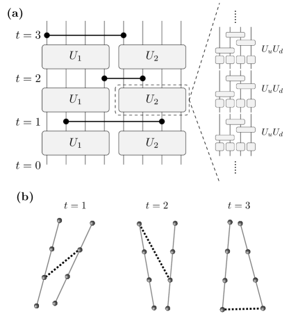
Figure 1: Sketch of the setup studied in this paper. (a) Two subsystems evolve independently from each other with respect to unitaries $U_{1(2)}$, obtained from an elementary Floquet unitary with tunable disorder strength [80], e.g., $U_{2}=(U_{u}U_{d})^{N_{p}}$, applied $N_{p}$ times (see text for more details). Then a two-qubit gate, for instance a CZ gate, is applied to connect the subsystems. This completes one time step. The two positions used in different time steps for the connecting two-qubit gate vary randomly over the whole size of the subsystems. (b) We consider one-dimensional subsystems for simplicity. The dashed lines indicate examplary positions used for the connecting gate in different time steps. Our numerical results are obtained by averaging over random realizations of the initial product state, the unitaries $U$ (independent for each subsystem), and the position of the connecting two-qubit gate.

The central idea is to perform “circuit-cutting” (cf. [85, 86, 87, 88, 89]), i.e., dividing the whole system into smaller patches whose time evolutions are simulated independently of each other by a full Schrödinger approach. The individual patches should be chosen as large as possible in order to efficiently utilize the available memory. Anticipating our numerical example below, let us consider for concreteness a system with a total of $L$ spin-$1/2$ degrees of freedom (i.e., qubits). The memory requirements to store the full state $\ket{\psi(t)}$ would scale as $\sim 2^{L}$. On the other hand, splitting the system in two halves and simulating the subsystems individually, memory would only scale as $\sim 2\times 2^{L/2}=2^{L/2+1}$.

The splitting of the system into patches naturally comes at a price. In particular, for each gate that connects different patches, the number of independent “trajectories” grows exponentially. (This is reminiscent of Clifford+T gate simulators, where the computational costs grow exponentially with the number of non-Clifford gates [90].) Specifically, consider a system split in two halves, which interact via a two-qubit gate where one qubit is chosen from the first subsystem and the other qubit is chosen from the second subsystem. In general, such a two-qubit gate is a $4\times 4$ matrix which can be decomposed as [73],

$$\begin{pmatrix}A_{00}&A_{01}\\ A_{10}&A_{11}\end{pmatrix} =P_{0}\otimes A_{00}+P_{1}\otimes A_{11}$$

$$+\ket{0}\bra{1}\otimes A_{01}+\ket{1}\bra{0}\otimes A_{10}\ ,$$ (1)

where $P_{0}=\ket{0}\bra{0}$ and $P_{1}=\ket{1}\bra{1}$ are projections on the local basis states of the first qubit, and the $A$ are $2\times 2$ matrices (i.e., general one-qubit gates) acting on the qubit in the second subsystem. Note that we could have also switched the roles of subsystem one and two in this decomposition. For a given trajectory, a single term from the right hand side of Eq. (1) is applied, and the full action of the gate recovered by suitably combining all possible trajectories (see below). Thus, in the most general case, the number of trajectories to be simulated is $4^{t}$ where $t$ is the number of connecting two-qubit gates (we choose $t$ as the unit of time in our numerical examples, see also Fig. 1).

In this paper, we will consider two specific examples of two-qubit gates connecting different patches, which are relevant to NISQ applications. The first example is a controlled-$Z$ gate,

$$\text{CZ}=\text{diag}(1,1,1,-1)=P_{0}\otimes\mathbb{1}+P_{1}\otimes Z\ ,$$ (2)

where $Z$ is a Pauli matrix. The decomposition on the right hand side of Eq. (2) indicates that the simulation of subsystems interacting via CZ gates is less complex than the general case in Eq. (1). In particular, the number of trajectories to be simulated is only given by $2^{\#\text{CZ}}$. In practice, we will use parallelization to simulate trajectories on multiple processors. A processor is given one of $2^{\#\text{CZ}}$ bitstrings, which encodes a particular trajectory.

As a more challenging example, we will also consider subsystems connected by iSWAP gates,

iSWAP $$=P_{0}\otimes P_{0}+P_{1}\otimes P_{1}$$

$$+i\ket{0}\bra{1}\otimes\ket{1}\bra{0}+i\ket{1}\bra{0}\otimes\ket{0}\bra{1}\ ,$$ (3)

for which the number of trajectories is $4^{\#\text{iSWAP}}$.

The total state is obtained by combining the contributions in a Feynman-like fashion,

$$\ket{\psi}=\sum_{k,l}\psi_{kl}\ket{k}\ket{l}=\sum_{k,l}\sum_{{\bf j}}\psi_{k}^{({\bf j})}\psi_{l}^{({\bf j})}\ket{k_{\bf j}}\ket{l_{\bf j}}\ ,$$ (4)

where the j-sum runs over all independent trajectories, and the $k,l$-sums run over the $2^{L/2}$ basis states in the two subsystems respectively. As the states of the subsystems are evolved in time à la Schrödinger, the coefficients $\psi_{k}^{({\bf j})}$ and $\psi_{l}^{({\bf j})}$ are generally kept in memory, whereas the $2^{L}$ coefficients of the full state $\ket{\psi}$ typically entail prohibitive memory requirements. Therefore, it might be necessary to additionally store the $\psi_{k}^{({\bf j})}$ and $\psi_{l}^{({\bf j})}$ to hard drive, and construct the coefficients of $\ket{\psi}$ required to evaluate observables after the simulation.

Generalizing Eq. (4) to more than two patches is straightforward. Moreover, if a nonperfect accuracy is acceptable, computational resources can be saved by simulating only a smaller (randomly chosen) fraction of trajectories in Eq. (4). For more details on Schrödinger-Feynman simulations and state-of-the-art implementations, see [73, 72].

While impressive quantum-circuit simulations have been performed [56, 73, 72], it might be fair to say that the Schrödinger-Feynman method is less known in the qunatum many-body physics community. Bridging this gap is a goal of the present work.

Model and Observables.– A natural application of the Schrödinger-Feynman technique is a situation, where two relatively large (sub-)systems interact weakly with each other. For instance, one could think of a system that interacts with a bath or reservoir (although, here, the bath will not be infinite or even bigger than the system), but the system-bath interaction only occurs sporactically in time. While this setup might seem somewhat artificial, a similar model was recently considered in Ref. [81], where a strongly and a weakly disordered subsystem were brought into contact to study the effect of a thermal inclusion on the putative many-body localization transistion. Our model studied below is partially inspired by Ref. [81], although we stress that we here do not aim to quantitatively address the stability of MBL.

Our setup is sketched in Fig. 1. Specifically, we consider a system split into two subsystems. Each subsystem is chosen as a linear chain of length $L_{1}$, $L_{2}$ such that the total size of the system is $L=L_{1}+L_{2}$ (we actually consider $L_{1}=L_{2}=L/2$). The chain geometry is chosen for simplicity, but does not represent a conceptual limitation of the Schrödinger-Feynman technique. Each subsystem evolves individually in time with respect to a unitary that can be tuned between a weak and a strong disorder regime. At discrete points in time, both subsystems interact with each other via a CZ or iSWAP gate, where the two qubits in the two subsystems are chosen randomly at each point in time.

For the unitary evolution, we study a variant of the Floquet random-circuit model introduced in Ref. [80] in the context of many-body localization. One Floquet period is given by a unitary $U=U_{u}U_{d}$, where $U_{d}$ is build from one-qubit gates, $U_{d}=d_{1}\otimes d_{2}\otimes\cdots\times d_{L}$. Each $d_{\ell}$ is a diagonal matrix, obtained by drawing a $2\times 2$ random matrix (different for each subsystem and site $\ell$) from the circular unitary ensemble and diagonalizing it. The computational $Z$ basis thus corresponds to the eigenbasis of the $d_{\ell}$. Further, $U_{u}$ consists of nearest-neighbor two-qubit gates $u_{\ell}=\exp(iM_{\ell}/\alpha)$, which are applied in a randomly chosen sequence, $U_{u}=\Pi_{\ell}u_{\pi(\ell)}$, where $\pi$ denotes a permutation and $M_{\ell}\in\mathbb{C}^{4\times 4}$ is drawn from the Gaussian unitary ensemble. The disorder strength is controlled by the choice of $\alpha$, where a large $\alpha$ corresponds to strong disorder (one-qubit gates dominate), and a small $\alpha$ corresponds to weak disorder (two-qubit gates dominate). For more details on the MBL random-circuit model, see Refs. [80, 91].

In practice, we will generate random unitaries $U_{1}$ and $U_{2}$ (different for each subsystem), with potentially different disorder strength $\alpha_{1}$ and $\alpha_{2}$ and differerent orders of the two-qubit gates in $U_{u}$. The subsystems evolve individually for a number of Floquet periods before interacting via a CZ or iSWAP gate. That is, we will define one time step below as, e.g., $\ket{\psi(t+1)}=\text{CZ}U_{1}U_{2}\ket{\psi(t)}$, where $U_{1}=(U_{u,1}U_{d,1})^{N_{p}}$. The number of Floquet periods within the unitaries $U_{1}$ and $U_{2}$ are fixed to $N_{p}=10$ to mimic that the subsystems are strongly interacting and building up entanglement internally, while only weakly interacting with each other.

Our results are averaged over multiple random-circuit realizations with independently chosen $U_{d}$ and $U_{u}$ in each run, as well as randomly chosen positions of the qubits involved in the interactions between subsystems [Fig. 1 (b)], i.e., interpreting our setup again as a system and bath, the interactions with the bath can occur globally, but only sporadically in time. Let us also emphasize that the Schrödinger-Feynman approach is agnostic to the specific type of unitary time evolution. Instead of the random-circuit model, we could have equally well considered Hamiltonian time evolution of the two subsystems.

As an obervable, we consider the survival probability of some out-of-equilibrium initial state $\ket{\psi(0)}$ [92],

$${\cal L}(t)=\left|\braket{\psi(0)}{\psi(t)}\right|^{2}\ .$$ (5)

The initial state is chosen as a product state from the $Z$ basis, i.e., $\ket{\psi(0)}=\ket{k}\ket{l}$ [in the notation of Eq. (4)] with randomly chosen product states $\ket{k}$ and $\ket{l}$. Then, crucially, in order to evaluate ${\cal L}(t)$ in Eq. (5), only this single amplitude of the full time-evolved state $\ket{\psi(t)}$ is required, i.e., ${\cal L}(t)=|\sum_{\textbf{j}}\psi_{k}^{(\textbf{j})}(t)\psi_{l}^{(\textbf{j})}(t)|^{2}$ with $k,l$ fixed by the initial state. The subsystem-state coefficients $\psi_{k}^{(\textbf{j})}(t)$ and $\psi_{l}^{(\textbf{j})}(t)$, distributed over multiple processors which each handle a particular trajectory j, are collected at each time step and ${\cal L}(t)$ is calculated during runtime. Thus, saving the states of the subsystems to hard drive is not required, which makes ${\cal L}(t)$ particularly suitable for the Schrödinger-Feynman technique. In our simulations, we average ${\cal L}(t)$, as mentioned above, over different random-circuit realizations, as well as random choices of the initial product state $\ket{\psi(0)}$.

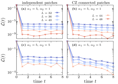
Figure 2: ${\cal L}(t)$ in circuits of size $L=L/2+L/2$. [(a),(b)] The first subsystem is strongly disordered with $\alpha_{1}=5$ while the second subsystem is weakly disordered with $\alpha_{2}=1$. [(c),(d)] Both subsystems are strongly disordered with $\alpha_{1,2}=5$. Panels (a) and (c), i.e., left column, show ${\cal L}(t)$ for the reference case of two independent subsystems (no connecting gates), while panels (b) and (d), i.e., right column show dynamics in the full interacting system with sporadic CZ gates connecting the two patches. The data for larger $L$ shows stronger fluctuations as it is averaged over fewer random-circuit realizations.

Results.– We now present our numerical results. In Fig. 2, the decay of ${\cal L}(t)$ is shown for two subsystems of size $L/2$ connected by sporadic CZ gates up to $t\leq 8$ (cf. Fig. 1 for the definition of one time step). We consider two different cases: (i) the dynamics of the first patch is strongly disordered with $\alpha_{1}=5$, while the second patch is only weakly disordered with $\alpha_{2}=1$ [Fig. 2 (a) and (b)]; (ii) both subsystems are strongly disordered with $\alpha_{1,2}=5$ [Fig. 2 (c) and (d)]. Moreover, in both cases, we compare ${\cal L}(t)$ in the fully interacting system, cf. Fig. 2 (b) and (d), to the reference case of having two independent subsystems, i.e., by removing the connecting CZ gates, cf. Fig. 2 (a) and (c).

Starting from ${\cal L}(0)=1$, we observe that most of the decay of ${\cal L}(t)$ happens during the first time step $t\leq 1$. Moreoever, comparing different system sizes up to $L\leq 48$, we find that especially for the weakly disordered case with $\alpha_{2}=1$, ${\cal L}(t)$ decreases approximately exponentially with $L$ as expected given the exponentially growing Hilbert space.

While most of the dynamics of ${\cal L}(t)$ is thus caused by the internal dynamics within the subsystems, we find that the sporadic interaction between the subsystems leads to a further slow decay of ${\cal L}(t)$ at $t>1$. This can be seen especially for $\alpha_{1}=\alpha_{2}=5$, where ${\cal L}(t)$ is essentially time-independent in the case of two disconnected patches [Fig. 2 (c)], while a monotonous decay of ${\cal L}(t)$ persists if the patches are connected to form a larger system [Fig. 2 (d)]. The coupling of the two subsystems mediated by the CZ gates thus allows $\ket{\psi(t)}$ to explore a larger Hilbert space even though the disorder strength is the same in both patches. This is consistent with the fact that signatures of thermalization (or potential localization) in disordered systems are subject to pronounced finite-size effects and require the simulation of large systems [17, 18, 19, 20, 21, 22, 23, 24].

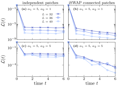
Figure 3: Analogous data as in Fig. 2, but now the two subsystems are connected by sporadic iSWAP gates.

Eventually, Fig. 3 presents analogous data, but now for subsystems connected by iSWAP gates. Due to their higher complexity, cf. Eq. (3), we only simulate dynamics in systems with $L\leq 40$ and up to a depth of $t\leq 6$, which corresponds to $4^{6}=2^{12}$ distinct trajectories, Comparing Fig. 2 and Fig. 3, it appears that using iSWAP gates leads to stronger “interactions” between the two subsystems as the monotonous decay of ${\cal L}(t)$ for $t\geq 1$ in Figs. 3 (b) and (d) is now even more pronunced. This can be understood from a physical point of view. In particular, CZ and iSWAP gates qualitatively differ from each in the sense that iSWAP gates can change the expectation values $\langle Z\rangle_{1}$ and $\langle Z\rangle_{2}$ of the total magnetization in the two subsystems, whereas $\langle Z\rangle_{1,2}$ is conserved under the application of a CZ gate. Note that in our numerical example, the unitaries $U_{1,2}$ in the Floquet circuit do not conserve $\langle Z\rangle_{1,2}$. However, one could imagine a similar random circuit with individual $U(1)$ symmetries in the two subsystems, cf. Ref. [93], or generate the dynamics instead by $e^{-iHt}$ with $H$ the standard MBL XXZ chain which is also $U(1)$-symmetric. For such cases, we expect that the thermalization-benefiting effect of the iSWAP gates would become even more pronounced (in comparison to the subsystem-particle-number-conserving CZ gates).

Figures 2 and 3 exemplify that the Schrödinger-Feynman technique allows us to study ${\cal L}(t)$ in systems with $L\leq 48$ with a Hilbert-space dimension of $\sim 10^{14}$, where we used parallelization with up to $256$ processes in an MPI architecture on a readily available central university computer cluster. In principle, from a memory and CPU number point of view, even larger systems and longer times would have been accessible for us. Note, however, that the here performed averaging over disorder realizations and initial states added another layer of computational complexity. Moreover, with comparable computational resources, standard sparse-matrix techniques would be restricted to systems of roughly half the size reached here.

Conclusions.– We have demonstrated the applicability of Schrödinger-Feynman simulations for questions in many-body quantum dynamics. Specifically, we have explored the decay of the pure-state survival probability in a disordered model (here in the form of a Floquet random circuit), where the strength of disorder is tunable such that one subsystems can act as a thermal bath for the other, cf. Ref. [81]. Studying large subsystems that interact sporadically in time, we have observed that signatures of thermalization become enhanced compared to the reference case of having two independent patches.

The system sizes of $L\leq 48$ reported here by no means represent the upper limit that can be managed by Schrödinger-Feynman techniques, see e.g., Ref. [72]. With the ever increasing availability of memory and processors, it should be possible in the future to push these methods to even larger subsystems with more connecting gates.

While our work is supposed to be a proof-of-principle demonstration, we hope that it will motivate the usage of Schrödinger-Feynman techniques in the quantum-dynamics community. Promising settings, as hinted at in this paper, are subsystems that are highly entangled internally, yet only interact weakly with each other, e.g., systems embedded in a bath, where the weak system-bath coupling can effectively be modelled by interactions that occur sparsely in time, which might also include certain impurity problems [94]. Moreover, while we here considered one-dimensional subsystems, more complicated geometries, for which no other efficient numerical methods may exist, can readily be treated within the same framework.

We thank Yaodong Li for useful discussions. J. R. acknowledges funding from the European Union’s Horizon Europe research and innovation programme, Marie Skłodowska-Curie grant no. 101060162, and the Packard Foundation through a Packard Fellowship in Science and Engineering (V.  Khemani’s grant). The simulations were carried out on Leibniz Universität Hannover’s computer cluster, funded by the Deutsche Forschungsgemeinschaft (DFG, German Research Foundation) – no. INST 187/592-1 FUGG, INST 187/742-1 FUGG.

References

- Nauts and Wyatt [1983] A. Nauts and R. E. Wyatt, Physical Review Letters 51, 2238 (1983).
- Long et al. [2003] M. W. Long, P. Prelovšek, S. El Shawish, J. Karadamoglou, and X. Zotos, Physical Review B 68, 235106 (2003).
- Aoki et al. [2014] H. Aoki, N. Tsuji, M. Eckstein, M. Kollar, T. Oka, and P. Werner, Reviews of Modern Physics 86, 779 (2014).
- Goth and Assaad [2012] F. Goth and F. F. Assaad, Physical Review B 85, 085129 (2012).
- Wurtz et al. [2018] J. Wurtz, A. Polkovnikov, and D. Sels, Annals of Physics 395, 341 (2018).
- Carleo and Troyer [2017] G. Carleo and M. Troyer, Science 355, 602 (2017).
- Schmitt and Heyl [2018] M. Schmitt and M. Heyl, SciPost Physics 4, 013 (2018).
- Schmitt and Heyl [2020] M. Schmitt and M. Heyl, Physical Review Letters 125, 100503 (2020).
- White et al. [2017] I. G. White, B. Sundar, and K. R. A. Hazzard https://doi.org/10.48550/arXiv.1710.07696 (2017).
- Mallayya and Rigol [2018] K. Mallayya and M. Rigol, Physical Review Letters 120, 070603 (2018).
- Guardado-Sanchez et al. [2018] E. Guardado-Sanchez, P. T. Brown, D. Mitra, T. Devakul, D. A. Huse, P. Schauß, and W. S. Bakr, Physical Review X 8, 021069 (2018).
- Richter and Steinigeweg [2019] J. Richter and R. Steinigeweg, Physical Review B 99, 094419 (2019).
- Vidal [2004] G. Vidal, Physical Review Letters 93, 040502 (2004).
- White and Feiguin [2004] S. R. White and A. E. Feiguin, Physical Review Letters 93, 076401 (2004).
- Haegeman et al. [2011] J. Haegeman, J. I. Cirac, T. J. Osborne, I. Pižorn, H. Verschelde, and F. Verstraete, Physical Review Letters 107, 070601 (2011).
- Paeckel et al. [2019] S. Paeckel, T. Köhler, A. Swoboda, S. R. Manmana, U. Schollwöck, and C. Hubig, Annals of Physics 411, 167998 (2019).
- Weiner et al. [2019] F. Weiner, F. Evers, and S. Bera, Physical Review B 100, 104204 (2019).
- Šuntajs et al. [2020a] J. Šuntajs, J. Bonča, T. Prosen, and L. Vidmar, Physical Review E 102, 062144 (2020a).
- Šuntajs et al. [2020b] J. Šuntajs, J. Bonča, T. Prosen, and L. Vidmar, Physical Review B 102, 064207 (2020b).
- Kiefer-Emmanouilidis et al. [2021] M. Kiefer-Emmanouilidis, R. Unanyan, M. Fleischhauer, and J. Sirker, Physical Review B 103, 024203 (2021).
- Panda et al. [2020] R. K. Panda, A. Scardicchio, M. Schulz, S. R. Taylor, and M. Žnidarič, EPL (Europhysics Letters) 128, 67003 (2020).
- Sierant et al. [2020] P. Sierant, D. Delande, and J. Zakrzewski, Physical Review Letters 124, 186601 (2020).
- Sels and Polkovnikov [2021] D. Sels and A. Polkovnikov, Physical Review E 104, 054105 (2021).
- Abanin et al. [2021] D. Abanin, J. Bardarson, G. De Tomasi, S. Gopalakrishnan, V. Khemani, S. Parameswaran, F. Pollmann, A. Potter, M. Serbyn, and R. Vasseur, Annals of Physics 427, 168415 (2021).
- White et al. [2018] C. D. White, M. Zaletel, R. S. K. Mong, and G. Refael, Physical Review B 97, 035127 (2018).
- Ye et al. [2020] B. Ye, F. Machado, C. D. White, R. S. Mong, and N. Y. Yao, Physical Review Letters 125, 030601 (2020).
- Rakovszky et al. [2022] T. Rakovszky, C. W. von Keyserlingk, and F. Pollmann, Physical Review B 105, 075131 (2022).
- Klein Kvorning et al. [2022] T. Klein Kvorning, L. Herviou, and J. H. Bardarson, SciPost Physics 13, 080 (2022).
- Zaletel et al. [2015] M. P. Zaletel, R. S. K. Mong, C. Karrasch, J. E. Moore, and F. Pollmann, Physical Review B 91, 165112 (2015).
- Kloss and Bar Lev [2019] B. Kloss and Y. Bar Lev, Physical Review A 99, 032114 (2019).
- Schuckert et al. [2020] A. Schuckert, I. Lovas, and M. Knap, Physical Review B 101, 020416 (2020).
- Hubig and Cirac [2019] C. Hubig and J. I. Cirac, SciPost Physics 6, 031 (2019).
- Czarnik et al. [2019] P. Czarnik, J. Dziarmaga, and P. Corboz, Physical Review B 99, 035115 (2019).
- Kloss et al. [2020] B. Kloss, D. Reichman, and Y. Bar Lev, SciPost Physics 9, 070 (2020).
- Richter et al. [2020] J. Richter, T. Heitmann, and R. Steinigeweg, SciPost Physics 9, 031 (2020).
- Kshetrimayum et al. [2020] A. Kshetrimayum, M. Goihl, and J. Eisert, Physical Review B 102, 235132 (2020).
- Richter et al. [2023] J. Richter, O. Lunt, and A. Pal, Physical Review Research 5, l012031 (2023).
- Osborne and Nielsen [2002] T. J. Osborne and M. A. Nielsen, Physical Review A 66, 032110 (2002).
- Schollwöck [2005] U. Schollwöck, Reviews of Modern Physics 77, 259 (2005).
- Eisert et al. [2010] J. Eisert, M. Cramer, and M. B. Plenio, Reviews of Modern Physics 82, 277 (2010).
- Preskill [2018] J. Preskill, Quantum 2, 79 (2018).
- Nielsen and Chuang [2012] M. A. Nielsen and I. L. Chuang, Quantum Computation and Quantum Information: 10th Anniversary Edition (Cambridge University Press, 2012).
- Chan et al. [2018] A. Chan, A. De Luca, and J. Chalker, Physical Review Letters 121, 060601 (2018).
- Bertini et al. [2019] B. Bertini, P. Kos, and T. Prosen, Physical Review Letters 123, 210601 (2019).
- Claeys and Lamacraft [2021] P. W. Claeys and A. Lamacraft, Physical Review Letters 126, 100603 (2021).
- Potter and Vasseur [2022] A. C. Potter and R. Vasseur, Entanglement dynamics in hybrid quantum circuits, in Entanglement in Spin Chains (Springer International Publishing, 2022) pp. 211–249.
- Lunt et al. [2022] O. Lunt, J. Richter, and A. Pal, Quantum simulation using noisy unitary circuits and measurements, in Entanglement in Spin Chains (Springer International Publishing, 2022) pp. 251–284.
- Li et al. [2018] Y. Li, X. Chen, and M. P. A. Fisher, Physical Review B 98, 205136 (2018).
- Skinner et al. [2019] B. Skinner, J. Ruhman, and A. Nahum, Physical Review X 9, 031009 (2019).
- Zhou and Nahum [2020] T. Zhou and A. Nahum, Physical Review X 10, 031066 (2020).
- von Keyserlingk et al. [2018] C. von Keyserlingk, T. Rakovszky, F. Pollmann, and S. Sondhi, Physical Review X 8, 021013 (2018).
- Nahum et al. [2018] A. Nahum, S. Vijay, and J. Haah, Physical Review X 8, 021014 (2018).
- Khemani et al. [2018] V. Khemani, A. Vishwanath, and D. A. Huse, Physical Review X 8, 031057 (2018).
- Fisher et al. [2023] M. P. Fisher, V. Khemani, A. Nahum, and S. Vijay, Annual Review of Condensed Matter Physics 14, 335 (2023).
- Mi et al. [2021] X. Mi, P. Roushan, C. Quintana, S. Mandrà, J. Marshall, C. Neill, F. Arute, K. Arya, J. Atalaya, R. Babbush, J. C. Bardin, R. Barends, J. Basso, A. Bengtsson, S. Boixo, A. Bourassa, M. Broughton, B. B. Buckley, D. A. Buell, B. Burkett, N. Bushnell, Z. Chen, B. Chiaro, R. Collins, W. Courtney, S. Demura, A. R. Derk, A. Dunsworth, D. Eppens, C. Erickson, E. Farhi, A. G. Fowler, B. Foxen, C. Gidney, M. Giustina, J. A. Gross, M. P. Harrigan, S. D. Harrington, J. Hilton, A. Ho, S. Hong, T. Huang, W. J. Huggins, L. B. Ioffe, S. V. Isakov, E. Jeffrey, Z. Jiang, C. Jones, D. Kafri, J. Kelly, S. Kim, A. Kitaev, P. V. Klimov, A. N. Korotkov, F. Kostritsa, D. Landhuis, P. Laptev, E. Lucero, O. Martin, J. R. McClean, T. McCourt, M. McEwen, A. Megrant, K. C. Miao, M. Mohseni, S. Montazeri, W. Mruczkiewicz, J. Mutus, O. Naaman, M. Neeley, M. Newman, M. Y. Niu, T. E. O’Brien, A. Opremcak, E. Ostby, B. Pato, A. Petukhov, N. Redd, N. C. Rubin, D. Sank, K. J. Satzinger, V. Shvarts, D. Strain, M. Szalay, M. D. Trevithick, B. Villalonga, T. White, Z. J. Yao, P. Yeh, A. Zalcman, H. Neven, I. Aleiner, K. Kechedzhi, V. Smelyanskiy, and Y. Chen, Science 374, 1479 (2021).
- Arute et al. [2019] F. Arute, K. Arya, R. Babbush, D. Bacon, J. C. Bardin, R. Barends, R. Biswas, S. Boixo, F. G. S. L. Brandao, D. A. Buell, B. Burkett, Y. Chen, Z. Chen, B. Chiaro, R. Collins, W. Courtney, A. Dunsworth, E. Farhi, B. Foxen, A. Fowler, C. Gidney, M. Giustina, R. Graff, K. Guerin, S. Habegger, M. P. Harrigan, M. J. Hartmann, A. Ho, M. Hoffmann, T. Huang, T. S. Humble, S. V. Isakov, E. Jeffrey, Z. Jiang, D. Kafri, K. Kechedzhi, J. Kelly, P. V. Klimov, S. Knysh, A. Korotkov, F. Kostritsa, D. Landhuis, M. Lindmark, E. Lucero, D. Lyakh, S. Mandrà, J. R. McClean, M. McEwen, A. Megrant, X. Mi, K. Michielsen, M. Mohseni, J. Mutus, O. Naaman, M. Neeley, C. Neill, M. Y. Niu, E. Ostby, A. Petukhov, J. C. Platt, C. Quintana, E. G. Rieffel, P. Roushan, N. C. Rubin, D. Sank, K. J. Satzinger, V. Smelyanskiy, K. J. Sung, M. D. Trevithick, A. Vainsencher, B. Villalonga, T. White, Z. J. Yao, P. Yeh, A. Zalcman, H. Neven, and J. M. Martinis, Nature 574, 505 (2019).
- Kim et al. [2023] Y. Kim, A. Eddins, S. Anand, K. X. Wei, E. van den Berg, S. Rosenblatt, H. Nayfeh, Y. Wu, M. Zaletel, K. Temme, and A. Kandala, Nature 618, 500 (2023).
- Keenan et al. [2023] N. Keenan, N. F. Robertson, T. Murphy, S. Zhuk, and J. Goold, npj Quantum Information 9, 72 (2023).
- Pednault et al. [2017] E. Pednault, J. A. Gunnels, G. Nannicini, L. Horesh, T. Magerlein, E. Solomonik, E. W. Draeger, E. T. Holland, and R. Wisnieff https://doi.org/10.48550/arXiv.1710.05867 (2017).
- Huang et al. [2021] C. Huang, F. Zhang, M. Newman, X. Ni, D. Ding, J. Cai, X. Gao, T. Wang, F. Wu, G. Zhang, H.-S. Ku, Z. Tian, J. Wu, H. Xu, H. Yu, B. Yuan, M. Szegedy, Y. Shi, H.-H. Zhao, C. Deng, and J. Chen, Nature Computational Science 1, 578 (2021).
- Gray and Kourtis [2021] J. Gray and S. Kourtis, Quantum 5, 410 (2021).
- Pan and Zhang [2022] F. Pan and P. Zhang, Physical Review Letters 128, 030501 (2022).
- Pan et al. [2022] F. Pan, K. Chen, and P. Zhang, Physical Review Letters 129, 090502 (2022).
- Ayral et al. [2023] T. Ayral, T. Louvet, Y. Zhou, C. Lambert, E. M. Stoudenmire, and X. Waintal, PRX Quantum 4, 020304 (2023).
- Tindall et al. [2023] J. Tindall, M. Fishman, M. Stoudenmire, and D. Sels https://doi.org/10.48550/arXiv.2306.14887 (2023).
- Liao et al. [2023] H.-J. Liao, K. Wang, Z.-S. Zhou, P. Zhang, and T. Xiang https://doi.org/10.48550/arXiv.2308.03082 (2023).
- Begušić et al. [2024] T. Begušić, J. Gray, and G. K.-L. Chan, Science Advances 10, https://doi.org/10.1126/sciadv.adk4321 (2024).
- Rudolph et al. [2023] M. S. Rudolph, E. Fontana, Z. Holmes, and L. Cincio https://doi.org/10.48550/arXiv.2308.09109 (2023).
- Anand et al. [2023] S. Anand, K. Temme, A. Kandala, and M. Zaletel https://doi.org/10.48550/arXiv.2306.17839 (2023).
- Kechedzhi et al. [2024] K. Kechedzhi, S. Isakov, S. Mandrà, B. Villalonga, X. Mi, S. Boixo, and V. Smelyanskiy, Future Generation Computer Systems 153, 431 (2024).
- Aaronson and Chen [2016] S. Aaronson and L. Chen https://doi.org/10.48550/arXiv.1612.05903 (2016).
- Chen et al. [2018] Z.-Y. Chen, Q. Zhou, C. Xue, X. Yang, G.-C. Guo, and G.-P. Guo, Science Bulletin 63, 964 (2018).
- Markov et al. [2018] I. L. Markov, A. Fatima, S. V. Isakov, and S. Boixo https://doi.org/10.48550/arXiv.1807.10749 (2018).
- Burgholzer et al. [2021] L. Burgholzer, H. Bauer, and R. Wille, in 2021 IEEE International Conference on Quantum Computing and Engineering (QCE) (IEEE, 2021) p. 199.
- Gopalakrishnan et al. [2015] S. Gopalakrishnan, M. Müller, V. Khemani, M. Knap, E. Demler, and D. A. Huse, Physical Review B 92, 104202 (2015).
- Nandkishore [2015] R. Nandkishore, Physical Review B 92, 245141 (2015).
- De Roeck and Huveneers [2017] W. De Roeck and F. Huveneers, Physical Review B 95, 155129 (2017).
- Goihl et al. [2019] M. Goihl, J. Eisert, and C. Krumnow, Physical Review B 99, 195145 (2019).
- Sels [2022] D. Sels, Physical Review B 106, l020202 (2022).
- Morningstar et al. [2022] A. Morningstar, L. Colmenarez, V. Khemani, D. J. Luitz, and D. A. Huse, Physical Review B 105, 174205 (2022).
- Peacock and Sels [2023] J. C. Peacock and D. Sels, Physical Review B 108, l020201 (2023).
- De Raedt et al. [2007] K. De Raedt, K. Michielsen, H. De Raedt, B. Trieu, G. Arnold, M. Richter, T. Lippert, H. Watanabe, and N. Ito, Computer Physics Communications 176, 121 (2007).
- De Raedt et al. [2019] H. De Raedt, F. Jin, D. Willsch, M. Willsch, N. Yoshioka, N. Ito, S. Yuan, and K. Michielsen, Computer Physics Communications 237, 47 (2019).
- Boixo et al. [2017] S. Boixo, S. V. Isakov, V. N. Smelyanskiy, and H. Neven https://doi.org/10.48550/arXiv.1712.05384 (2017).
- Peng et al. [2020] T. Peng, A. W. Harrow, M. Ozols, and X. Wu, Physical Review Letters 125, 150504 (2020).
- Barratt et al. [2021] F. Barratt, J. Dborin, M. Bal, V. Stojevic, F. Pollmann, and A. G. Green, npj Quantum Information 7, 79 (2021).
- Bravyi et al. [2016] S. Bravyi, G. Smith, and J. A. Smolin, Physical Review X 6, 021043 (2016).
- Mitarai and Fujii [2021] K. Mitarai and K. Fujii, New Journal of Physics 23, 023021 (2021).
- Gentinetta et al. [2024] G. Gentinetta, F. Metz, and G. Carleo, Quantum 8, 1296 (2024).
- Bravyi and Gosset [2016] S. Bravyi and D. Gosset, Physical Review Letters 116, 250501 (2016).
- Ha et al. [2023] H. Ha, A. Morningstar, and D. A. Huse, Physical Review Letters 130, 250405 (2023).
- Torres-Herrera and Santos [2015] E. J. Torres-Herrera and L. F. Santos, Physical Review B 92, 014208 (2015).
- Jonay et al. [2022] C. Jonay, J. F. Rodriguez-Nieva, and V. Khemani https://doi.org/10.48550/arXiv.2210.13429 (2022).
- Sun and Chan [2016] Q. Sun and G. K.-L. Chan, Accounts of Chemical Research 49, 2705 (2016).