Free Zero Bias and Infinite Divisibility
Larry Goldstein***larry@math.usc.edu1, Todd Kemp†††tkemp@ucsd.edu2,
1Department of Mathematics, University of Southern California, Los Angeles
2Department of Mathematics, University of California, San Diego
Abstract.
The (classical) zero bias is a transformation of centered, finite variance probability distributions, often expressed in terms of random variables , characterized by the functional equation
where is the variance of . The zero bias distribution is always absolutely continuous, and supported on the convex hull of the support of . It is related to Stein’s method, and has many applications throughout probability and statistics, most recently finding new characterization of infinite divisiblity and relation to the Lévy–Khintchine formula.
In this paper, we define a free probability analogue, the free zero bias transform acting on centered random variables, characterized by the functional equation
where denotes the free difference quotient. We prove existence of this transform, and show that it has comparable smoothness and support properties to the classical zero bias. Our main theorem is an analogous characterization of free infinite divisibility in terms of the free zero bias, and a new understanding of free Lévy measures. To achieve this, we develop several new operations on Cauchy transforms of probability distributions that are of independent interest.
1. Introduction
The zero bias transform was introduced in [18] as a component of Stein’s method [32],[13] for normal approximation. Given a random variable with law in (the set of probability measures on with mean zero and variance ), there exists a unique distribution defined by the property that, for a random variable with law ,
| (1.1) |
Here is the class of all infinitely differentiable functions with compact support. The associated mapping with domain has the Gaussian as its unique fixed point (i.e. reproducing the usual Gaussian integration by parts formula that motivates the Stein equation). This and related transformations (such as size bias) have found uses in normal approximation [13], concentration inequalities [10], [12], [17], [22] and data science [14], [24], [25], [21], [15]. In a forthcoming preprint [20], the authors discovered an interesting connection between the zero bias and infinite divisibility: a distribution with mean and finite variance is infinitely divisible if and only if where are independent and is uniform on ; here denotes equality in distribution.
The purpose of the present paper is to introduce the free probability analog of the zero bias transform, which we call the free zero bias (or correspondingly for random variables ), also on the set . We can extend the transformation to variables with non-zero mean , as is in Theorem 5.1, by
| (1.2) |
that is, by applying the transformation to the centered variable , and then adding back in.
We define the putative free zero bias for mean zero variables by the following characterizing equation, analogous to (1.1):
| (1.3) |
That is to say: the ordinary derivative in (1.1) is replaced in (1.3) by the difference quotient
This substitution forms a core plank of “free harmonic analysis”. It ultimately arises from perturbation theory (of eigenvalues), or more simply from the relationship between derivatives and functional calculus. If is a single-variable polynomial, it can act as a function on matrices, or more generally as a function on any Banach algebra by functional calculus: if then for any . Then the function is smooth, and its ordinary Fréchet derivative (a linear map acting on elements ) is actually given by the two-variable polynomial acting on (on both sides), evaluated at ; see [30, Proposition 4.3.1] and [31, Example 6.5]. To be more precise: is a function of two variables; the quantity on the right-hand-side of Equation (1.3) should be interpreted as for two (classically) independent random variables both having law . In other words,
This non-linear definition appears quite complicated, but as summarized in Theorem 1.1 below, the equation does uniquely determine a nice probability measure.
We let denote weak convergence of a sequence of probability measures.
Theorem 1.1.
Given any and probability measure in , there is a unique probability measure on that satisfies Equation (1.3) with and . This measure is called the free zero bias; we also refer to any random variable with distribution as a free zero bias of .
The free zero bias has the following properties:
-
a)
The unique fixed point of is the semicircle law of mean and variance , with density .
-
b)
For any mean zero with finite, non-zero variance, the free zero bias is absolutely continuous with respect to Lebesgue measure and
-
c)
The support of is contained in the convex hull of the support of .
-
d)
The free zero bias transform is continuous: if converges weakly and , then converges weakly.
The existence claim of Theorem 1.1 and part a) follow by the Cauchy transform based on Definition 3.8 of the free zero bias and Lemma 3.12; b) and c) are shown in Theorem 4.1; and d) is part c) of Lemma 3.9.
It is convenient to write the difference quotient in the form
| (1.4) |
where is a Uniform random variable on ; if, for a smooth , we choose to define on the diagonal as , this identity holds for all including . A priori, Equation (1.3) requires the two variable function to be defined on the diagonal, and so we may canonically make the above choice when . That being said: due to Theorem 1.1 part b), always has an absolutely continuous distribution, and as such, the diagonal values of do not affect the value of .
Remark 1.2.
Taking test functions and comparing (1.1) and (1.3) in light of (1.4), we see the following relationship between the (classical) zero bias and the free zero bias:
| (1.5) |
where is a uniform random variable on (classically) independent from and . This equivalence is proved carefully as (3.19) in Lemma 3.12 and will be useful below in Sections 3 and 4.
A number of benefits of the classical zero bias is a consequence of its key ‘replace one property’ that allows one to construct the zero bias of a sum of independent variables by replacing a single summand. We derive the free analog in Theorem 3.14. Though its form is somewhat more complex, it still expresses the (free) zero bias of a sum in terms of the (free) zero bias of a single summand.
As noted above, the (classical) zero bias transformation was shown in [20] to give, via the ‘replace one property’, an insightful characterization of infinitely divisible probability distributions on the real line. Our main application of our free zero bias (in Section 5) proves analogous results and offers new insights on freely infinitely divisible distributions.
Recall that a random variable is (classically) infinitely divisible if, for each , there exists a distribution such that
| (1.6) |
In the 1930s Kolmogorov, and then independently Lévy and Khintchine, proved the following: a finite-variance random variable is infinitely divisible if and only if there exist and a probability measure on , known as the Lévy measure, such that the characteristic function of satisfies
| (1.7) |
and furthermore that is unique when . In [20] it is shown that (1.7) holds if and only if on a possibly enlarged probability space there exists a uniform random variable, and such that
| (1.8) |
and in this case, the measure in (1.7) and the distribution of in (1.8) correspond. See also [33] for a similar result for non-negative, integrable infinitely divisible random variables and their relation to the size bias transformation.
In free probability, the central role of the characteristic function is played instead by the Cauchy transform
where denotes the upper half plane . The Cauchy transform is defined and analytic on , and it will occasionally be useful to consider it on the lower half plane as well. Note that the function depends on only through its law: if then
As such, we refer to as convenient. The law is fully characterized by , and the relationship is robust and continuous; see Section 2 below for details.
In classical probability, the cumulant-generating function is the logarithm of the characteristic function; it has the essential property of linearizing independence: if (and only if) and are independent. An analog of this construction in free probability is the -transform in which the law is encoded, which satisfies if and only if and are freely independent. The functional relationship between and is more complicated than the simple logarithmic relationship in the classical context: for in an appropriate domain (discussed below),
| (1.9) |
It is useful to simultaneously use “reflected” versions of both the Cauchy transform and the -transform: The reciprocal Cauchy transform , and the Voiculescu transform that satisfies . Equation (1.9) can then equivalently be written as
| (1.10) |
Free infinite divisibility is defined as in (1.6) with (classical) independence of the summands replaced by free independence; see Section 2. In [4], Bercovici and Voiculescu proved that a random variable with mean is freely infinitely divisible if and only if its -tranform is of the form
| (1.11) |
for some measure on ; this is the free analog of the Kolmogorov–Lévy–Khintchine formula (1.7). In fact, [4] proved an even more general result: for any freely infinitely divisible random variable (whether it has finite mean or not) there is a finite measure and a constant such that
| (1.12) |
In the case that has two finite moments, one can work out that the measure satisfies (1.11), where .
One of the main results of the present paper, Theorem 1.5 below, is a more probabilistic characterization of the measure in (1.11). It turns out that is a finite measure if and only if has two finite moments, in which case the mass of is the variance of . To avoid trivial cases where is constant, we may assume that the variance of is positive.
Proposition 1.3.
Let be a random variable with finite mean and variance . Then is freely infinitely divisible if and only if there is a random variable such that
| (1.13) |
We refer to the law as the Lévy measure of .
Moreover: for every probability measure on , and every and , there is a unique freely infinitely divisible random variable with mean , variance , and Lévy measure — i.e. so that (1.13) holds with .
The first claim of this proposition follows from Theorem 1.5 below and the relation between the and Voiculescu transformations, while the final claim of the proposition is shown in Theorem 5.8.
Remark 1.4.
The free Lévy–Khintchine formula (1.13) shows that the Lévy measure is symmetric iff is symmetric. Indeed, is symmetric if and only if, for
where the penultimate equality follows from the assumption ; the reverse implication follows from the Stieltjes inversion formula, cf. Proposition 2.2. Reciprocating, the same holds for , and using (1.10), it follows that is symmetric iff on its domain. Since , the equivalence of symmetry for and follows from (1.13). This equivalence will be useful in several examples below.
Equation (1.13) is equivalent to the form given in Theorem 13.16 in [29], where it is left as an exercise (using combinatorial methods) to derive it in the special case that has compact support. Our main theorem gives a third equivalent characterization of free infinite divisibility for random variables, stated in terms of the free zero bias. Moreover, it gives a probabilistic interpretation for what the Lévy measure of actually is: namely, it is the limit of the square biases of “th root” distributions of .
Theorem 1.5.
Let be any probability measure on . There is a unique probability measure whose Cauchy transform satisfies . If has distribution , we let denote a random variable with distribution .
Let be a random variable with mean and variance . The following are equivalent.
-
a)
is freely infinitely divisible.
-
b)
There is a random variable so that the Voiculescu transform has the form
-
c)
Recalling (1.2), the free zero bias of satisfies
(1.14)
In the case that these equivalent statements hold true, the law of is uniquely identified as follows. As is freely infinitely divisible, it can be expressed as where , are freely independent identically distributed with common law . Then the weak limit of the sequence of square biased distributions (cf. Definition 3.5) exists and equals .
The first assertion of Theorem 1.5 (the existence of ) is proved in Lemma 3.4; together with the existence of the free zero bias, this result follows from a curious result, Lemma 3.2, which states that the geometric mean of two Cauchy transforms of probability measures is again the Cauchy transform of some probability measure; this result may be of independent interest.
The equivalence of the three conditions for free infinite divisibility in Theorem 1.5 and the representation of as a weak limit is the subject of Section 5, culminating with Theorem 5.10. As item b) is equivalent to the free Kolmogorov–Lévy–Khintchine formula (1.11), the equivalence of a) and b) (without the assumption of two finite moments for ) was proved in [4]. We provide a new, self-contained proof here, in the specific context of finite-variance, that crucially identifies the Kolmogorov–Lévy–Khintchine measure in (1.11): rescaling by the variance, it is the law of where is the random variable appearing in c). This outcome is achieved by connecting the relation (1.14) to the -transform in Theorem 5.1, and then probabilistically identifying the measure in (1.11) as the distributional limit of the ‘square bias’ distributions of the freely independent and identically distributed summands that produce . Under a compact support condition a more direct, and self contained proof, is provided in Theorem 5.12.
Remark 1.6.
Written in terms of characteristic functions, (1.8) states that a centered random variable is (classically) infinitely divisible if and only if its (classical) zero bias satisfies . Comparing this identity with (1.14), we consider pre-composing with to be the free version of multiplying with ; in particular, is a free version of multiplying with a (classically) independent uniform random variable. It would be interesting to express the operation in more direct probabilistic terms, i.e. using operations on (free) random variables, rather than transforms of their distributions.
Our work is related to that of [9] and [16], where Stein kernels, familiar in classical probability [8, 11], are shown to also exist in free probability. Classically, we say that is a Stein kernel for having distribution when
| (1.15) |
We note that (1.15) is similar to (1.1) in that it modifies Stein’s original identity for the normal by changing some feature on the right hand side, for (1.1) the distribution of , and for (1.15) the multiplier of the derivative of . When the distribution of is absolutely continuous with respect to with Radon-Nikodym derivative , then from (1.1) and the change-of-variables theorem,
In particular, under the stated absolute continuity requirement, provides a Stein kernel.
The notion of a Stein kernel in free probability was first introduced in [16], and used to obtain a free counterpart of the HSI inequality, connecting entropy, Stein discepancy and free Fisher information, as well as a rate of convergence in the entropic free central limit theorem. The work [9] shows that free Stein kernels, unlike in the classical case, always exist. It shows in addition that free Stein kernels are never unique by providing two constructions that lead to distinct results, one inspired by an unpublished note of Giovanni Peccati and Roland Speicher in the case where the potential is and where , and a second one constructed via the Reisz representation theorem.
For a single random variable , we say that is a Free Stein kernel for when
| (1.16) |
where is a (classically) independent copy of . A relation similar to the one in the classical case holds between free Stein kernels and the free zero bias. Indeed, when the distribution of is absolutely continuous with respect to with Radon–Nikodym derivative , from (1.3) and the change-of-variables theorem we have
| (1.17) |
Comparing with (1.16), we see, as in the classical case under a similar absolute continuity assumption, that free zero bias provides a free Stein kernel, here given by , which has the form of a product of some function of multiplied by the same function of .
In the setting of (1.16), the first of the two distinct Stein kernels discussed in [9] corresponds to , for which (1.16) is nearly immediately verified to hold upon applying the definition of the difference quotient and the fact that . This kernel must be distinct from the one in (1.17) generated by the free zero bias, as cannot be written in the necessary product form. The construction of the second kernel in [9] requires that satisfies the free Poincaré inequality. However, no such requirement is needed for the kernel for in (1.17).
This work is organized as follows. The remainder of this introduction, in Section 2, is devoted to a brief primer on free probability, in particular as it relates to analytic transforms. In Section 3 we prove the existence of the free zero bias transformation by demonstrating a more general result regarding taking the geometric means of Cauchy transforms, and introduce other needed transforms, along with some basic properties and examples. In particular, Theorem 3.14 in that section provides the free analog of the classical key ‘replace one’ property. In Section 4 we show that, like the classical zero bias, the free version always has an absolutely continuous distribution. In Section 5 we consider infinitely divisible random variables. These sections are essentially independent of each other and can be read in any order.
2. A Free Probability Primer
Free probability is a noncommutative probability theory introduced by Voiculescu in the late 1980s and early 1990s, initially with the intent to import core ideas from probability, statistics, and information theory to solve structure and isomorphism problems in operator algebras. Through its intimate connection with random matrix theory, it has grown over the last three decades into a flourishing field of study on its own. The reader may wish to consult [29, 27] for detailed treatises on free probability.
The arena is a noncommutative probability space , which replaces the algebra of bounded random variables and the expectation functional on them in the classical case. is a unital -algebra, like the algebra of complex matrices for example, where the adjoint operation is conjugate transpose. (Note: to avoid notational conflict with the (classical) zero bias of (1.1), for the rest of this section we use to refer to the adjoint operation rather than .) is a state: a linear functional satisfying that is positive in the sense that, for any other than , . As the notation suggests, should be thought of as expectation; indeed, if is the algebra of bounded random variables on some probability space, then the expectation is the standard choice for . Some authors prefer to use a letter like or for the state functional in free probability; we will use throughout.
For some results (which we will need), more assumptions are required. A -probability space is a noncommutative probability space where is a von Neumann algebra (a weakly closed subalgebra of the algebra of bounded operators on a Hilbert space), and is tracial: for all , and also continuous in the weak∗ topology (identifying the algebra with its predual). This latter continuity condition, sometimes called normal continuity, is designed to make a version of the Dominated Convergence Theorem hold for ; in particular, an equivalent statement is that, for any bounded increasing net of positive operators , . We will make these assumptions going forward, for convenience. Typical examples are matrices equipped with the normalized trace; any classical probability space; and various standard type von Neumann algebras. As with classical probability, one doesn’t typically work in some particular explicit (noncommutative) probability space; the random variables (i.e. elements of ) are assumed to “live” on a space with enough structure to make the usual results work, and that typically means a probability space.
The free in free probability refers to a noncommutative “independence” notion for random variables. Algebraically, statistical independence of random variables (corresponding to joint laws being product measures) corresponds to tensor product; in free probability, the independence rule is instead modeled on free product from group theory. Ultimately, it is best to express it as a moment-factoring condition. For classical bounded random variables, independence can be stated combinatorially as the exepctation factoring property for all . This equality will also hold for freely independent random variables, but it is not sufficient: when random variable multiplication is noncommutative, this rule doesn’t handle expressions like . To handle such expressions, freeness is most easily stated in terms of subalgebras.
Definition 2.1.
Let be a noncommutative probability space. A collection of unital -subalgebras of is called freely independent if the following holds true: given indices that are consecutively distinct (i.e. , , etc.) and random variables that are centered (i.e. ), the product is also centered, that is, .
We say random variables are freely independent if the -subalgebras they generate are freely independent.
For our purposes, it is only necessary to deal with selfadjoint variables . For a selfadjoint , the -algebra it generates is just the set of all polynomial functions of it, . For such variables, then, free independence can be expressed a bit more directly: selfadjoint are freely independent if, given any consecutively distinct indices , and polynomials such that , it follows that . By using the usual centering trick, applying this property to variables , one learns that free random variables satisfy the usual factoring property , as well as a litany of more complex noncommutative factoring properties, for example . In general, if random variables are freely independent, any mixed moment can be expressed (as a polynomial function) in terms of the variables’ individual moments.
Another benefit of selfadjoint variables is that, like classical random variables, they have probability distributions. Associated to each selfadjoint in a probability space there is a unique probability measure on sharing the same moments:
Mirroring the classical setting, we denote as the law of . Existence follows from the spectral theorem for selfadjoint operators: associated to is a projection-valued Borel measure on such that , and then functional calculus of is given by (which is consistent with analytic functional calculus when is analytic, e.g. a polynomial). Composing with the state on both sides yields , showing that is the desired law.
For the moment, we restrict to the probability space context, meaning that the random variables are bounded operators on a Hilbert space. This implies that their distributions are compactly-supported (we will discuss removing this requirement shortly), and hence uniquely determined by their moments, which establishes uniqueness of the law. Moreover, any compactly-supported probability distribution arises this way (just take any classical random variable with law ). A deeper result is that any collection of compactly-supported probability measures can be coupled together as the laws of freely independent random variables on a common space (see Definition 2.1). This leads to a new operation on such measures, free convolution . The measure is defined to be the law of where and are freely independent with laws and respectively. To see this is well defined, we look at moments. The moments of are all linear combinations of mixed moments in and , which in turn factor in terms of moments of and separately. Ergo, the moments of are completely determined by the moments of and separately. Unlike the classical case, there is no simple integral formula for in terms of and ; but there is an approach using analytic transforms which we now describe.
As mentioned on page 1, for a probability measure on , its Cauchy transform is the analytic function defined by
| (2.1) |
If is a selfajoint random variable, then from the definition (above) of its law, we have
where the function is real analytic on for any . This reflects the change-of-variables formula in classical probability. When convenient, we may write this as .
Any Cauchy transform is an analytic map from the upper half plane into the lower half plane . (Since is a real measure, the domain of can really be taken as , and , hence it also maps into .) The Cauchy transform also satisfies as , and these conditions characterize Cauchy transforms: if is an analytic map from into satisfying as , then is the Cauchy transform of a unique probability measure on . More generally, the asymptotic behavior of Cauchy transforms holds along any path with that stays well clear of the real line (i.e. in a cone).
The Cauchy transform of a probability measure completely characterizes , and moreover this relationship is robust under weak limits. The following is a complex analysis exercise; a detailed proof can be found in [23, Section 8].
Proposition 2.2.
Let be a probability measure on , with Cauchy transform . The Stieltjes inversion formula recovers from as the weak limit as , where has real analytic density
Let be a sequence of probability measures on .
-
(1)
If for some probability measure , then converges to uniformly on compact subsets of .
-
(2)
Conversely, if converges pointwise to a function that is analytic on , then for some finite measure with , and converges vaguely to .
The domain of invertibility of a Cauchy transform will be important in our analysis. For , the truncated cone (also known as a Stolz angle) is
Then for any path with (and this also characterizes Cauchy transforms). It is often convenient to work with the reciprocal Cauchy transform mentioned above: ; which is an analytic self-map of the upper half plane satisfying for large in some . This asymptotic behavior suggests that (and hence ) is an invertible function for sufficiently large , and this is indeed true.
Proposition 2.3 (Proposition 5.4 in [4]).
If is any probability measure on , and , then for any , there exists some such that is univalent in (i.e. is one-to-one and has an analytic inverse), with range .
That is: on a sufficiently truncated cone, has an analytic inverse whose domain includes a truncated cone arbitrarily close to the domain of .
On an appropriate truncated cone, is an analytic map, and given that , the same holds true for . The Voiculescu transform , introduced on page 1, is defined, a priori on some truncated cone , by
| (2.2) |
This function satisfies as in . Moreover, this convergence (and the given truncated cone) is robust under weak convergence of measures.
Proposition 2.4 (Proposition 5.7 in [4]).
A sequence of probability measures on converges weakly to some probability measure if and only if there are such that all converge uniformly on compact subsets of to a function and uniformly in as , . In this case, in .
The key property of the Voiculescu transform is that it linearizes free independence:
for all in an appropriate truncated cone. This was proved for compactly-supported measures, the only kind for which the combinatorial definition (Definition 2.1) of freeness makes sense a priori, in [34]. Later it was shown [26, 4] that for any probability measures on , there is a unique probability measure such that in a truncated cone; this allows the extension of free convolution to all probability measures, defining . To be clear: is defined by computing and (each determined completely by its measure, through and ), summing, and then computing on an appropriate truncated cone. By Proposition 2.3 and the above-mentioned papers, the inverse of this function coincides with reciprocal Cauchy transform of a unique probability measure on a closely related truncated cone. This function has an analytic continuation to all of , and then (taking reciprocal) the measure can be recovered via the Stieltjes inversion formula.
From Proposition 2.3, the domain of can be taken as a truncated cone for any (given large enough ); and the conjugate symmetry implies the vertical reflection in the lower half plane can be included as well. Correspondingly, the domain of can always be taken as an open disk centered at the origin with narrow regions along the real axis removed. In fact, if is compactly-supported, the domain is actually an open disk, and the -transform is analytic. Its Taylor coefficients at the origin are polynomial functions of the moments of , called the free cumulants; indeed, the first three are the classical cumulants (mean, variance, skewness), while they disagree from the fourth on. The -transform is the free analog of the cumulant-generating function (i.e. the log-characteristic function). Its relation to the Cauchy transform is expressed in (1.9). Note that, from its simple relation to the Voiculescu transform, we have .
Remark 2.5.
As with the Cauchy transform and its reciprocal, we abuse notation with the Voiculescu transform and -transform and write and , for a (potentially unbounded) selfadjoint random variable . This gives the concise statement that two random variables are freely independent if and only if .
Like the Cauchy transform (Proposition 2.2), free convolution is robust under weak limits.
Proposition 2.6 (Proposition 5.7 in [4]).
Let be probability measures on , and suppose and . Then .
The -transform and Voiculescu transform of are easily described in terms of those of and separately, but the implicit relationship between these and the Cauchy transform makes it harder to compute directly with . There is a function relating them, known as the subordinator.
Proposition 2.7 (Proposition 4.4 in [35]; Theorem 3.1 in [7]; Proposition 7.3 in [5]).
Let be probability measures on . There is a unique analytic function that satisfies
Moreover
If , are freely independent random variables, we denote .
In principal, these properties follow simply from the defining relation of the subordinator, which can informally be written as . Using Proposition 2.3, this rigorously defines on an appropriate truncated cone, but the key to the use of subordinators is their analyticity on the whole upper half plane.
Like Cauchy transforms (and other analytic transforms defined above), subordinators are robust under weak convergence. This fact is apparently folklore in the literature; we provide a simple proof outline below.
Proposition 2.8.
If and are sequences of probability measures with weak limits , , then uniformly on compact subsets of .
Proof.
By Proposition 2.4 there is a fixed truncated cone on which converges uniformly on compact subsets to . By Propositions 2.2 and 2.6, converges to uniformly on compact subsets of . What’s more, converges uniformly on compact subsets of another fixed truncated cone . Note that the intersection is another truncates cone. Let be an open subset with compact closure ; thus converges uniformly on .
Appealing to the definition (2.2), , and thus the preimage of under is . As converges uniformly, there is thus a fixed non-empty open set with for all . Hence, .
Applying (2.2) once more,
is defined and analytic on since maps into . The composition thus converges to uniformly on compact subsets of the open subset of the upper half plane. Since and are all analytic in the full upper half plane, the proposition now follows from Montel’s theorem. ∎
The main place we will need to use subordinators is to compute conditional expectation in a free probabilistic context. If is a -probability space, and is a von Neumann subalgebra, then there is a conditioning map . As in the classical case, it can be constructed as an -projection. It is a linear map, which satisfies the following two key properties:
-
(1)
If and , then .
-
(2)
If , then for any , .
If is freely independent from , then is constant; this mirrors the same result which holds classically if is independent from . However, things diverge significantly between the classical and free worlds, as we’ll see shortly.
If is a random variable in , and if is the von Neumann subalgebra generated by (in the selfadjoint case this can be interpreted as the set of all measurable bounded functions of , ), then we typically denote . This is relevant for the present work in the case of computing where is a smooth bounded test function and are freely independent. If were classically independent, this is simply equal to where for ; but that is not true in the free world. Instead, we have the following important result.
Proposition 2.9 (Theorem 3.1 in [7]).
Let and be freely independent selfadjoint random variables with laws and . Let be the Feller–Markov kernel whose Cauchy transform is given by
| (2.3) |
Then for any bounded Borel measurable function ,
| (2.4) |
In particular: fixing , the function is bounded and continuous; (2.3) and (2.4) together then say
| (2.5) |
A probability measure on is called freely infinitely divisible (or -infinitely divisible) if, for each , there is a probabiliy measure such that . Equivalently, is freely infinitely divisible if, for each , is the -transform of a probability measure. By taking convolution powers, this means that has the form for some probability measure for any rational ; a continuity result [4, Lemma 5.9] then shows that this holds for all real as well. Thus, freely infinitely divisible measures correspond to free convolution semigroups satisfying for , and (the original measure is then identified as ). A major result identifying such measures/semigroups is [4, Theorem 5.10], which states that a measure is freely infinitely divisible if and only if (and hence ) has an analytic continuation to all of (which may take values in ). That same theorem also proves the free Kolmogorov–Lévy–Khintchine formulas (1.11) and (1.12).
Remark 2.10.
Curiously, in the free world, every probability measure is in a partial free convolution semigroup as . In other words, for , is always the -transform of a probability measure . This was fully proved in [1, Theorem 2.5(1)] using subordinator methods, generalizing earlier results [2, 28] in the compactly supported case. This is one of many places where free probability has intriguingly different properties from classical probability.
3. Existence and properties of the Free Zero Bias Distribution
In Section 3.1 we first prove the existence of a distributional transformation based on the fact that the a “geometric mean” of two Cauchy transforms of probability measures is again the Cauchy transform of a probability measure, cf. Lemma 3.2. In Section 3.2 we use a special case of Lemma 3.2 to produce a new measure transformation we call the El Gordo transform, and we also review the square bias transformation and provide some of its properties. Combining these in Section 3.3 then yields the construction of the free zero bias putatively defined by (1.3), and the proof that its unique fixed point is the semi-circle distributions. Finally, in Section 3.4 we consider a few examples.
3.1. Geometric Mean Transformation
Complex square roots will come up frequently in this section and beyond, so we begin by setting notation.
Notation 3.1.
For , the (principal) square root is defined uniquely in polar coordinates: writing for and , . The function is holomorphic on the slit plane , with image contained in the upper half plane .
Note that if and then ; but if are in the lower half plane, then . Similarly, if is in the slit plane, then . Finally: note that if , then is in the slit plane.
With the square root in hand, the following elementary Lemma yields a (surprisingly) new operation on probability distributions.
Lemma 3.2.
Given any two random variables and , there is a unique probability measure (which we denote as the law of a new random variable ) whose Cauchy transform satisfies
| (3.1) |
I.e. is the “geometric mean” of the Cauchy transforms of and . The map is bi-continuous in the sense that whenever and , as .
Proof.
and are analytic maps from to , hence for any the product defines an analytic function taking values in the slit plane . Hence is analytic, and takes values in the lower half plane . That it is equal to follows from the second paragraph in Notation 3.1.
Hence, to show that is the Cauchy transform of a probability measure, it suffices to verify that as . For this, we appeal to the second representation in (3.1). Since and are Cauchy transforms of probability measures, and , and therefore and as . Since is continuous and takes values in , the function is also continuous, and hence ; similarly . Hence
and we conclude that , showing that is the Cauchy transform of a probability measure as claimed, and uniqueness follows from Stieltjes inversion (cf. Proposition 2.2.
Example 3.3.
-
a)
For any random variable ,
i.e. .
-
b)
Consider the case that and are constants; e.g. and . Then
(3.2) (The last equality comes from Notation 3.1, since when .) Now employing the Stieltjes inversion formula (Proposition 2.2), the law can be recovered, and possesses a density:
(3.3) That is to say: the law of in (3.3) is the arcsine distribution on . More generally, letting and be point masses at respectively, scaling and translating appropriately we obtain
which is the arcsine distribution on .
-
c)
We can combine any random variable with a point mass this way, producing a new distribution whose Cauchy transform is . This construction, with , will be very important through the remainder of the paper, so we address it in the next result.
3.2. The Square Bias and El Gordo Transformations
In this section, we introduce one old (square bias ) and one new (El Gordo ) transformation on probability measures, focusing on their actions on Cauchy transforms. We begin with El Gordo.
Lemma 3.4.
For any probability measure ,
| (3.4) |
is the Cauchy transform of a probability distribution. We call the El Gordo transform of . This transformation on the set of all probability measures is continuous in the topology of convergence in distribution, has point mass at zero as its unique fixed point, satisfies for all , and is injective but not surjective.
Proof.
As , we find that , and the existence and continuity properties follow by Lemma 3.2. That is the map’s unique fixed point follows immediately by solving the equality , implying either or which is not the Cauchy transform of a probability measure.
Next, if we have that as the left hand side is zero with probability since the El Gordo transform takes to . When then
Taking square roots gives , and this implies by the Stieltjes inversion formula, cf. Proposition 2.2.
To show that the El Gordo transform is injective, when the distributions of and are equal, then
and squaring both sized and multiplying by implies , and yielding by the Stieltjes inversion formula.
To show that the map is not surjective, we show that no point mass, other than zero, is in the range of the El Gordo transform. Indeed, if , meaning that , it follows that
Note, however, that is then a positive multiple of
Hence, unless , the above function maps the half-disk of radius in the upper half plane back into the upper half plane, and so the putative is not the Cauchy transform of a probability measure. ∎
We now review the square bias transform, which also enters into the study of the zero bias in the classical case, see e.g. [13].
Definition 3.5.
Let be the law of an random variable . If let , a point mass at zero, and otherwise have distribution with Radon-Nikodym derivative with respect to that of given by
| (3.5) |
We call the square bias transform of .
In Theorems 5.5 and 5.8 we will also have need to consider the following pseudo-inverse of the square bias tranforms.
Definition 3.6.
If , let . If then let the distribution have Radon-Nikodym derivative with respect to that of given by
| (3.6) |
The next lemma collects many useful properties of the square bias.
Lemma 3.7.
Let and be square integrable random variables.
-
a)
Let and
Then , and when then
(3.7) -
b)
When , and satisfy and , then
-
c)
If is a sequence of square integrable random variables such that and , then The restriction that the second moment of the limit be positive is necessary.
-
d)
When the Cauchy transform of is given by
-
e)
For all we have .
-
f)
If then
Proof.
-
a)
The expression given for is clear from the representation of as a mixture. Under the assumption , applying Definition 3.5 for any bounded continuous yields
(3.8) As at least one of must be positive, without loss generality, by relabelling and if necessary, we may assume and are both positive. If then and the second term in the numerator of (3.8) is zero, producing , in agreement with (3.7), whose second term likewise vanishes.
When , then continuing from (3.8) we obtain the claim by
(3.9) -
b)
First suppose that . Note that this common distribution cannot be point mass at zero, being excluded by the condition .
Letting be a measurable subset of not containing zero and , we obtain
(3.10) Specializing to we obtain
thus showing the left and right hand sides of (3.10) are equal for all measurable . The other direction of the claim follows from part a).
-
c)
As converges to a positive limit, for all greater than some , the second moments of are strictly positive.
For any bounded continuous function ,
where for taking the limit in the numerator we use that is uniformly integrable and hence so is , by the boundedness of .
If takes on the value with probability , and is otherwise zero, then where and , but, by part a) takes the value with probability one, and hence does not converge in distribution to zero, showing the necessity of the positivity condition.
-
d)
Applying the definition of the Cauchy transform and of , and then adding and subtracting yields
yielding the claim.
-
e)
When , then either or , and in both cases both sides of the claimed identity are equal to point mass at zero. Otherwise, for a given bounded measurable function , letting , we have
- f)
∎
3.3. Construction of the Free Zero Bias
We now arrive at the main construction: the free zero bias. To motivate it, we return for a moment to the classical zero bias which is defined by the functional equation (1.1). There is a probabilistic construction of : first take its square bias , and then multiply it by an independent random variable ; that is,
The proof can be found in [19, Theorem 2.1]. In particular, this construction appears in (12) of that work when specializing to the case and , upon noting that the random variable whose distribution is given in (11) has the distribution by virtue of the fact that defined in (10) is equal to in this case.
One may wonder if some version of this statement, with independence replaced by free independence and uniform replaced by some other distribution perhaps, might characterize the free zero bias of (1.3). While nothing of this nature has presented itself, the following definition does have the same flavor, and (as we see shortly) works.
Definition 3.8.
Note: the free zero bias, like the square bias and El Gordo transforms it is composed of, acts only on probability measures; throughout this paper, we have it act on random variables by acting on their laws, and abuse notation writing (as above) rather than .
Here are several important properties of the free zero bias, including a concrete formula for its Cauchy transform.
Lemma 3.9.
The free zero bias defined above satisfies the following properties.
-
a)
if and only if .
-
b)
For all we have .
-
c)
If and , then .
-
d)
The Cauchy transform of satisfies
(3.13)
Proof.
For a), if have the same law then the same holds for via Definition 3.8. Conversely, as the El Gordo transform is injective by Lemma 3.2, whenever are equally distributed the same is true for . Next, for b), note that by Lemma 3.4 and e) of Lemma 3.7, for all ,
For the next claim, part c) of Lemma 3.7 shows that the assumed convergence conditions on imply that , so the claim follows by the distributional continuity of the El Gordo transform provided by Lemma 3.2.
Remark 3.10.
Remark 3.11.
Neither the square bias or El Gordo transforms require centered random variables, and indeed Definition 3.8 makes perfect sense for all random variables, centered or not. All the properties in Lemma 3.9 parts a), b), and c) hold true if , while the reader can readily verify that (3.13) is replaced more generally with
| (3.14) |
Nevertheless, as mentioned in (1.2), where has mean , we define
| (3.15) |
noting that this definition is in agreement with the previous one in the case . Extending the definition in this way preserves the fixed point property of the transformation, as explored in Example 3.16(c).
However, the mean condition is required for the defining functional equation to hold, in both the classical and free cases. In comparison to the classical case: if is independent from then is a random variable, but it only coincides with when .
We now show the main reason why the free zero bias transformation is of interest. We will find it convenient to work with resolvent functions
| (3.16) |
These functions are bounded and smooth on .
We recall that the semi-circle law with mean zero and variance has Cauchy transform
| (3.17) |
Lemma 3.12.
For any the mapping with domain has the semi-circle law with variance as its unique fixed point, and for all
| (3.18) |
for all Lipshitz functions , and
| (3.19) |
where and are independent, and .
Proof.
Setting in (3.13) of Lemma 3.9 yields
implying that via (3.17). For the second claim, letting be a resolvent function for a given , and using (3.13), we have
Now, from (3.16),
This shows that (3.18) holds for all .
Now, for all such , using (1.5) and rewriting in terms of the derivative of and an independent , we obtain
Letting , we have therefore shown that for all . Since , we have
where the final equality (differentiating under the integral) follows because and are continuous on a neighborhood of each point . Similarly, . Hence, we’ve established that for all , which means and differ by a constant, which must be since both Cauchy transforms are near . Hence , and by the Stieltjes inversion formula, it follows that , establishing (3.19).
∎
Remark 3.13.
In the classical world, much of the success that the zero bias transformation enjoys is due to what can be called ‘the replace one property’. The following lemma gives its free analog; we include the classical one for the sake of comparison. For a clearer parallel, we extend the scope of the classical zero bias to general mean random variables, as in (3.15).
In what follows, we adopt the definition of the classical for non-mean zero random variables juas as was done in (1.2) for the free case.
Theorem 3.14.
Consider variables with means and finite, non-zero variances , and sum where . For , let be a random index with distribution .
When the summand variables are classically independent, and is independent of where is independent of and has the zero-bias distribution, then given by has the -zero bias distribution, and the characteristic function of satisfies
| (3.20) |
When the summand variables are freely independent, then the Cauchy transform of satisfies
| (3.21) |
When the summands are identically distributed as , these relations respectively specialize to
| (3.22) |
Remark 3.15.
As a reminder: is the subordinator function introduced in Proposition 2.7 by the relation for when are freely independent. Here and are indeed freely independent, since all the are free from each other. Subordinators connect Cauchy transforms of free sums, in an analogous (but more complicated) manner to the simple multiplicative relationship between characteristic functions of independent sums. It is therefore natural for them to appear in the free analog of “the replace one property”.
Proof.
For a proof of (3.20) in the mean zero case, see [18]. Using that result in the third equality, and with , in the general mean case we have
For the free case, this same type of reasoning, and the simply proved fact that
allows us to reduce to the mean zero case. Next, noting (using (3.16)) for any random variable with independent copy , and any that
| (3.23) |
Now, let and be the probability measures of and respectively. Using (3.23) with , (3.18) of Lemma 3.12, and the definition of , we have
For the terms in this sum, we use (free) conditioning (see Section 2) as follows:
where the second equality follows from (2.5) and the third is just the definition of in (3.16). Applying again the functional equation (3.18), the last expression is equal to
which follows again by (3.23). Summing up, we have therefore shown that
and dividing through by yields (3.21). The final statement of the theorem, in the identical distribution case, follows immediately as in this case and for all . ∎
3.4. Transform Examples
Example 3.16.
-
a)
We consider two examples of computing the free zero bias for distributions that do not have mean zero, and compare to the result given by (3.14), which agrees with the free zero bias in the mean zero case.
For the first example consider the semi-circle distribution with mean zero and variance one, and let for . Using (3.17) with and
identity (3.14) yields
Computing the free zero bias of from (3.15), and using that , we obtain
thus confirming that is a fixed point, and hence
We see that these two expressions are not equal.
-
b)
For a second example of a different nature, consider mixtures of point masses at zero and at some non-zero value ,
Then , and shifting the distribution to have mean zero we have
We find that , and hence
Therefore
and now taking the El Gordo transformation produces
and adding the mean back in we obtain
(3.24) corresponding to the arcsine distribution on .
- c)
We recall that to compute either the classical or free zero bias of a mean zero the first step is to compute , followed by multiplying by an independent in the classical case. That multiplication in the free case is replaced by taking the El Gordo transformation. We note that has the distribution, while the standard arcsine, of which all examples here are scaled and shifted versions via Example 3.3, has the distribution.
Example 3.17.
Taking one further iterate of the free zero bias distribution of the Rademacher considered in Example 3.16, the free zero bias distribution of the arcsine law on , having mean zero and variance , has Cauchy transform
Using Stieltjes inversion (Proposition 2.2), we evaluate and let . Note that and this number is in the lower half plane when ; thus, its square root has negative real part, in particular for . Similarly when . Now evaluating, we see that converges as to real values when , meaning that such points are outside the support of . Meanwhile, in the interval , the formula for the imaginary part of the complex square root yields the density
| (3.25) |
4. Absolute Continuity of the Free Zero Bias
In this section, we prove that the free zero bias of any distribution is absolutely continuous with respect to Lebesgue measure on , with support contained in the convex hull of the support of . The (classical) zero bias of any distribution has a density with respect to Lebesgue measure, and is supported within the convex hull of the support of , cf. [18]. The following result proves this also holds for the free zero bias, and moreover provides a quantitative bound that was not previously known in the classical case; the remaining claims regarding can be found in [18] and [13].
Theorem 4.1.
Let and respectively be the classical and free zero bias of a mean zero probability measure with finite, non-zero variance . Then
| (4.1) |
and both and are absolutely continuous with respect to Lebesgue measure. It holds that , and .
Proof.
Let have law , and consider the case where . We first show that has no point masses. For the sake of contradiction, assume that takes on the value with non-zero probability . Then, in view of (1.5), from
where is an independent copy of , we see that with probability at least , in contradiction to the absolute continuity of the distribution, see [18]. Recalling , as has a continuous distribution, we have that with probability zero, hence the value along the diagonal of double integrals such as (4.3) below, with respect to the product measure , is zero.
With arbitrary, take . Then
| (4.2) |
Using that and (1.1), which also holds for Lipshitz functions [13], we find via (4.2) that
thus showing the first claim of (4.1) when .
For the second claim, dividing up the plane according to Figure 2, we first consider the (non-exhaustive) collection of cases
1-1\nsn \MULTIPLY2-1\nbn
1.251\ssn \MULTIPLY1.252\sbn \MULTIPLY1.25\nsn\snsn \MULTIPLY1.25\nbn\snbn
Using symmetry when interchanging and , we obtain
| (4.3) |
As the integrands are all non-negative, using (4.2) for the final inequality we obtain
showing (4.1) when .
Now turning to the support, letting , for we have
and hence
As in the first integrand, the first integral is non-negative and hence the right hand side is non-negative.
For any such that the left hand side above is zero, and hence both terms on the right are zero; in particular . Now let be such that , or, equivalently, that . Using the scaling property b) of Lemma 3.9 with yields we have that , showing that the support of is contained in .
For having measure with arbitrary variance , applying the case shown for the unit variance variable and using that yields
The argument for general in the free zero bias case (4.1) is identical.
The absolute continuity claims now follows, and the final one, regarding the support of follows from the unit variance case, and that for any we have if and only if . ∎
5. Infinite Divisibility
This section is devoted to the proof of Theorem 1.5, which connects the free zero bias to free infinite divisibility. The seminal papers [6] and [4] explore and characterize infinite divisibility in the free world in terms of a Lévy–Khintchine representation (1.11); our main contribution is to derive this same formula using the free zero bias, adding a third leg to existing characterizations of free infinite divisibility, and providing a new approach to the subject in the setting. Crucially, we also show that any finite measure corresponds through (1.11) to a unique (up to a choice of mean) freely infinitely divisible random variable whose variance is the mass of , and that the probability measure has a probabilistic interpretation connecting and its free zero bias : this probability measure is the law of the random variable in (5.1)-(5.3).
We begin in Section 5.1, which is encompassed largely by Theorem 5.1. This Theorem gives the “symbolic equivalence” expressed in Theorem 1.5 — i.e. the equivalence of (5.1), (5.2), and (5.3) on some truncated domains — with the majority of the remainder of the section devoted to extending the relations to the full upper half plane. To that end, Section 5.2 introduces a family of compound free Poisson distributions in Framework 1, all freely infinitely divisible, that are rich enough to instantiate all of those for which . Section 5.3 then begins by removing this negative second moment constraint with an approximations scheme (therefore going beyond the compound free Poisson world) in Theorem 5.8, and then to complete the pieces of the proof of Theorem 1.5 in Theorem 5.10. Finally, Section 5.4 gives an alternate approach to Theorem 5.8 under the stronger assumption of bounded random variables; this approach is more self-contained, and also introduces a result, Lemma 5.11, on the uniformity of the support of free convolution roots that is of independent interest. Throughout the section, and at its conclusion, are several examples demonstrating the computational effectiveness of our new perspective on free infinite divisibility.
5.1. Symbolic Equivalent Formulations of Free Infinite Divisibility
In this section we develop relations between the four types of transforms associated with a distribution which are connected to the form of Cauchy transform of . In particular, Theorem 5.1 affirms the equivalence of relation (5.1), involving a reciprocal Cauchy transform depending on , to (5.2) and (5.3), specifying the forms of the and Voiculescu transforms of on certain truncated cone domains. The equivalences are those required to yield those between b) and c) in Theorem 1.5, once extended to all of .
Theorem 5.1.
Let be a mean random variable with variance , and a random variable. The following are equivalent.
| (5.1) |
for .
| (5.2) |
for in a reciprocal truncated cone.
| (5.3) |
for in a truncated cone.
If these equivalent conditions hold for both the pairs and then , and if for both pairs and then, assuming without loss of generality,
where, for any , is the -fold free convolution of .
See Remark 2.10 for a discussion of free convolution powers for .
Proof.
To begin, note that from the definitions (1.9) and (2.2) of the -transform and the Voiculescu transform. Applying this identity in (5.2) and using
we see that (5.3) is simply the statement of (5.3) with replaced by , yielding the equivalence. Moreover, we may reduce to the case . Indeed, if we know that (5.1) holds for mean zero variables then
and if (5.3) holds for mean zero variables, then since , we find
Hence we may assume without loss of generality.
Now, suppose that (5.3) holds in some truncated cone in the domain of ; under the assumption this is the statement . From the definition (2.2), and hence on . Letting for , we have , and so
Multiplying through by and noting yields
| (5.4) |
where the first equality is given by (3.13) and the last equality is given by (3.4). The equality implies that , since any Cauchy transform satisfies (not ) as . Taking reciprocals verifies (5.1) for , which is open (since is open and is continuous). Thus, the two analytic functions and are equal on an open set, and hence open on their full domain as claimed. The reverse implication (5.1)(5.3) is proved in exactly the same manner in reverse.
Turning to the second half of the theorem: When either identity is satisfied for then is uniquely determined by its Voiculescu transform in (5.3), which depends only on the distribution of , which itself encodes the mean. When both and satisfy either, and therefore both, of the given identities for the same , by (5.2) we must have
and hence
thus yielding the final claim. ∎
Example 5.2.
When is a distribution with zero mean, we know by Lemma 3.12 that the solution to is the semicircle distribution for some . In addition, this distribution must also satisfy (5.1) with , hence, by Lemma 3.4, with . In this case the (Lévy) measure in (5.2) is given by point mass at zero, implying the well-known fact that the -transform of a semicircle is given by . In particular is an -transform for all , and thus, as for all we have , the distribution of is infinitely divisible.
In the other direction, given the infinity divisibility of the semi-circle distributions and their corresponding -transforms , one can find their Lévy measures by (5.2). Indeed, from there we obtain
demonstrating that .
5.2. Free Compound Poisson Distributions
In this section we consider sequences of variables , for some , given by
| (5.5) |
The following result, though simple, will be used multiple times below.
Lemma 5.3.
If in (5.5) then , and if in addition then
Proof.
By the free independence and identical distribution assumption we have
and hence by Chebyshev’s inequality and the fact that , and the claim follows as convergence in probability and in distribution are equivalent when the limit is constant. ∎
We pay special attention to the case where the common summand distributions in (5.5) are generated by:
Framework 1.
Let and let be a random variable with law , mean and positive, finite second moment. Set
the distribution that puts mass on zero, and the remainder according to .
Under Framework 1, we show that the limits of produce instances where identities (5.1) and (5.2) can be shown to hold.
Lemma 5.4.
Proof.
For convenience, we drop the subscript . As , the sequence is uniformly integrable, and . Hence Lemma 5.3 obtains on the subsequence, and by the definition we have .
As , we conclude that . Therefore, by Proposition 2.8, it follows that uniformly on compact subsets of as . Since is freely independent from any random variable , by definition satisfies , and , so we conclude that
uniformly on compact subsets of as .
Theorem 5.5.
Remark 5.6.
Proof of Theorem 5.5:
First note that from [3, Theorem 3.4] there exists such that with ; this follows since the classical convolution version of this result was known since antiquity, and the variance is the same in both cases (variance is additive over classically independent or freely independent summands). The mean and variance claims for are easily verified. Now by Lemma 3.7(b) we have for all , and applying Lemma 5.4 with yields the first identity in (5.7), the second following by the equivalence granted in Theorem 5.1.
Next, we show that every function in the collection (5.8) is an -transform. The case yields -transforms of point masses on constants , so we may restrict to . As when is an -transform of a random variable the function is the transform of , it suffices to prove that each function for , as defined in (5.8), is an -transform.
For any such that , as this expectation cannot be zero, we may consider the distribution given by Definition 3.5, for which and by part f) of Lemma 3.7. In particular, the functions in (5.7) are -transforms for all . Varying over we see that is an -transform for any .
Consequently, any with -transform as in (5.8) is infinitely divisible as for any , replacing and by and produces an -transform, thus demonstrating that has a distributional root.
Example 5.7.
Setting , point mass at , and choosing some in Theorem 5.5, we obtain a Free Poisson variable in the limit, having mean and variance . As , and as (5.7) then yields , we conclude that the Cauhcy transform of satisfies
implying
and therefore that
thus identifying the distribution of as the Free Poisson. From Remark 5.6 we also obtain the transform of as
5.3. Free Infinite Divisibility
We now move to the general case of a freely infinitely divisible random variable with finite second moment. We begin with Theorem 5.8 that shows the expression in (5.9) is an transform of an infinitely divisible for any and for any random variable . This first step is accomplished by removing the restriction that in (5.8) in Theorem 5.5 by paralleling the argument showing Lemma 1.1.3 in [20] that proves an analog of this result in the classical case by constructing a sequence of variables approximating whose inverse second moment exists.
Following that step, we prove Theorem 5.10, which is the converse result to Theorem 5.8 completing our main result: that any freely infinitely divisible random variable gives rise to another random variable satisfying the relations (5.1)–(5.3), arising as the limit of the square bias transforms of the free convolutional roots of . Since the law of is the Lévy measure associated to , this gives a probabilistic interpretation of the free Lévy–Khintchine formula.
Theorem 5.8.
For any random variable , and , the function
| (5.9) |
is an -transform that corresponds to a freely infinitely divisible with mean and variance .
Proof.
As in the proof of Theorem 5.5, using the translation property of -transforms when adding a constants, it suffices to prove the result for .
When then , which is the transform of , and the result holds trivially.
Now take . When , in view of Example 5.2, is the transform of the semi-circle distribution, which is shown there to be freely infinitely divisible.
Hence, we restrict to the case where and . For let where we take small enough so that . Let and ; thus . Further, as , we may let as in Definition 3.5, so that by f) of Lemma 3.7.
Now we apply Theorem 5.5 with replaced by . This yields a limit, say , which has -transform
Reasoning exactly as in the proof of Theorem 5.5, we conclude that all of the functions of the form
are -transforms of probability measures. Similarly, for all and all ,
is a Voiculescu transform, whose domain manifestly has an analytic continuation to the whole complex plane, as it coincides on a truncated cone (an open set) with a scaled Cauchy transform. As as , by Proposition 2.2, converges to uniformly on compact subsets of , and hence converges uniformly on compact subsets of to the analytic function . What’s more, (the last inequality comes from the fact that for any Cauchy transform , as is easily verified using the triangle inequality in the definition (2.1)), and hence uniformly in . Therefore, it follows from Proposition 2.4 that the limit is the Voiculescu transform of some probability measure, and so is the -transform of that probability measure.
Letting we have
and as the sum of transforms is again an transform, we find that
is an -transform for any and . The mean and variance can be read off directly from (5.9).
An argument showing that the corresponding is infinitely divisible can now proceed exactly as in the proof of Theorem 5.5. ∎
Remark 5.9.
Theorem 5.10.
Let be a square integrable freely infinitely divisible random variable with mean and variance . For , let be the distribution of the freely independent, identically distributed summands satisfying . Then the weak limit of exists and uniquely satisfies (5.3).
Proof.
For readability, set . Using (3.4) defining and (3.13) defining , and squaring both sides, this yields
or equivalently
| (5.10) |
From Proposition 2.7, is uniquely determined by the equation
From Proposition 2.3 applied in sequence to and , for in an appropriate truncated cone this is equivalent to , and the range of this function contains another truncated cone . (These truncated cones a priori vary with ; since by Lemma 5.3, it follows from Proposition 2.4 that uniform truncated cones exist here.)
Let ; then for we equivalently have . Thus, for , (5.10) says
where the second equality comes from the fact that . As , converges to uniformly on compact subsets of by Proposition 2.2(1). Hence
| (5.11) |
uniformly on compact subsets of .
Taking stock: we have now used the “replace one” property, and the definitions of the square bias and free zero bias transforms, to show that the Cauchy transform of converges to the analytic function on some domain . We would like to use Proposition 2.2(2) to complete the proof of the theorem that converges in distribution to a probability measure. This requires two more steps: first we must show that the convergence in (5.11) occurs on all of , and then we must show that no mass is lost at infinity, that is, the resulting limit is a Cauchy transform with total mass .
For each , is analytic on all of ; similarly, since is freely infinitely divisible, is also analytic on all of (cf. [4, Theorem 5.10]). Since is an open subset of , it now follows from Montel’s theorem that converges to on all of (in fact uniformly on compact subsets). We therefore conclude by Proposition 2.2(2) that is the Cauchy transform of a finite measure with , and that the law of converges vaguely to . It remains only to show that (since a vaguely convergent sequence of probability measures whose limit is a probability measure converges in distribution). In other words, we merely need to show that as along some ray in the upper half plane.
To motivate this last step, consider what happens in the special case that is compactly supported. In this case, Speicher’s theory of free cumulants [29] gives a Taylor series expansion where and . Hence , and thence it follows immediately that as . To extend this argument rigorously to the more generally setting where need not be compactly supported, but only assumed to have two finite moments, we make use of some results due to Maassen [26].
is the reciprocal Cauchy transform of a probability measure on with finite variance and mean . Therefore, by [26, Proposition 2.2(b)] it follows that for some probability measure on . Thus, for ,
and hence
Multiplying both sides by yields
| (5.12) |
Now, again using only the fact that has mean and variance , [26, Lemma 2.4] yields that . Thus, along any path in with imaginary part tending to , the left-hand-side of (5.12) has the same limit as , while the right-hand-side tends to (since is the Cauchy transform of a probability measure). This concludes the proof that is a probability measure.
This concludes the proof of our main Theorem 1.5. To clarify how:
Proof of Theorem 1.5:
Theorem 5.10 shows that a) implies b) (by applying to the centered random variable and noting that ), Theorem 5.1 shows that b) implies c) and Theorem 5.8 shows that c) implies a).
5.4. The Compactly-Supported Case
The proof of Theorem 5.10 uses [4, Theorem 5.10]: the fact that the Voiculescu transform of a freely-infinitely divisible random variable has an analytic continuation to the whole upper half plane; the continuation is given by the Lévy–Khintchine formula itself, as in the statement of Theorem 1.5(b). We can avoid requiring a priori knowledge of this important fact, if we restrict to the case that is compactly-supported. To do so, we need the following ancillary result, which is of some independent interest, and may well be known in the literature but not in literature known to the authors.
Lemma 5.11.
Let be a compactly-supported probability measure on . There is a compact interval that contains the supports of all -convolution roots of . That is: for any , if is a probability measure satisfying , then is compactly supported with .
Proof.
To begin, note that we may safely assume is centered (which implies that is centered); otherwise we can center it by translating by the mean, which distributed to translating by its mean ( times the mean of ), then apply the result in the centered case and translate the intervals back.
So, let be a centered probability distribution, with support contained in a compact interval , and let denote its variance. For , since , we have the subordination relation where is the subordinator from to . In [1, Theorem 2.5(3)], the authors show that this subordinator has an elegant form:
| (5.13) |
(See also [36, Section 2.3] for a concise presentation.) For , = has a continuous extension to [1, Theorem 2.5(4)], so we may discuss the behavior of and on . From the Stieltjes inversion formula, is real-valued on .
By [26, Proposition 2.2(b)], since is the reciprocal Cauchy transform of a centered measure with variance , there is a probability measure on such that
and the continuity of on extends this relation similarly. Note that is real-valued on prescisely where is, and thus is also supported in . Equation 5.13 therefore becomes
Outside , the function is analytic, and for ,
In particular as , and so for ,
A similar analysis for shows that there.
In particular, if , . Since is continuous, it follows that its image on contains (and derivative calculations show that it is one-to-one there as well).
Hence every point has the form for some with , and so shows that is real since is real valued off . A similar argument shows that is real-valued on . This shows that the support of is contained in , as desired. ∎
Theorem 5.12.
Proof.
Since has compact support, by Lemma 5.11, the support of the summand distributions in (5.5), with replacing , are contained in a compact interval . As the distribution of is absolutely continuous with respect to that of by Definition 3.5, the supports of are also contained in . Any sequence of probability measures supported in the fixed compact interval is tight; hence every subsequence of has a limit (which a priori depends on the subsequence). As in (5.5) equals for all , the remaining hypotheses of Lemma 5.4 hold trivially, and invoking the lemma shows that (5.1) and (5.2) hold for the pair , and Theorem 5.1 shows is unique. Therefore, each subsequence has a convergent subsequence and all subsequential limits are the same ; it follows the full sequence must also converge to . ∎
5.5. Examples
We now come to the conclusion of this paper, showing how to use the results and techniques above to effectively compute new examples of freely infinitely divisible distributions.
Proposition 1.3 shows that for every law , every and every that there exists an infinitely divisible with whose -transform and Voiculescu transform are given by (1.13) (i.e. the free Lévy–Khintchine formula). Our main Theorem 1.5 gives an equivalent characterization in terms of the free zero bias, (1.14), which is an equation only involving (reciprocal) Cauchy transforms. This allows us to fairly easily produce new examples of freely infinitely divisible random variables by choosing any (and and ) and using (1.14) to derive an equation for the corresponding Cauchy transform . In practice, this equation can often be solved explicitly.
In general, the contribution of the mean is simply a shift. Indeed, from the definition (1.2) of the free zero bias, (1.14) says
Squaring both sides and using the definition (3.4) of the El Gordo transform and the definition (1.2) of the free zero bias (in the mean setting) yields the equation
and now noting that , we have for each and a one-parameter family of solutions for that are just translated by :
| (5.14) |
We will use (5.14) in the examples below, and restrict to the case since all other solutions are just translations.
Example 5.13.
Let have the centered semicircle distribution with variance , . From (5.14), we find that the mean , variance freely infinitely divisible distribution with Lévy measure satisfies
Isolating the square root on the right hand side and then squaring both sides, we obtain the quadratic equation
that simplifies to
| (5.15) |
Solving, and choosing the negative square root to produce the required cancellation (to yield ), we obtain
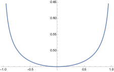
As , this function has a continuous extension to ; taking we see that is purely real if , and hence the density is given by
| (5.16) |
Note that we recover the semicircle density as the law of when , i.e. when the Lévy measure . Indeed, in this case Equation (5.15) reduces to which is the standard quadratic equation for the Cauchy transform of the semicircle law. This aligns with Example 5.2.
Example 5.14.
Let , a Rademacher distribution. Here
In this case (5.14) becomes
which simplifies to the cubic equation
| (5.17) |
While analytic expressions for the general solution to this cubic are tractable, they become much simpler in the case , where (5.17) becomes the depressed cubic equation
| (5.18) |
For the general depressed cubic equation with , the three solutions can be expresses as follows. Let be the cube root of unity in ; then
| (5.19) |
Here the square and cube roots are the principal branches. For our case of interest (5.18), and , so
| (5.20) |
To determine which of the three roots is the Cauchy transform we seek, we look at asymptotics: using Newton’s Binomial theorem (twice), we compute that
Hence, (5.19) yields
Note that if then , and so , hence is not a Cauchy transform. On the other hand, we see that , exhibiting the correct asymptotic behavior for a Cauchy transform of a probability measure. Since we know that one of the roots is , we conclude that it is , i.e.
| (5.21) |
with as given in (5.20).
Note that the quantity inside the cube root in is never ; as such, the function has a continuous extension to . Thus is a combination of a density and potentially a point mass at .
Recall that the cube root is the principal branch; thus, for a positive number , and hence
| (5.22) |
An analogous argument applied to , noting that , yields
| (5.23) |
Notice that, in this interval,
| (5.24) |
Hence
In light of (5.21), we can thence combine (5.22) and (5.23), and apply the symmetry principle of Remark 1.4, to yield the density
| (5.25) |
on the punctured interval .
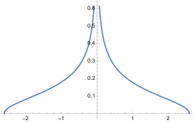
For , and so
An analogous calculation to (5.24), relying on the fact that and for , shows that
Hence, for , is real-valued, and therefore has no mass there.
Example 5.15.
Let have the Cauchy distribution, with density and, via a counter integral argument, Cauchy transform ; this distribution has no finite positive, nor negative, finite integer moments. The corresponding centered, variance freely infinitely divisible distribution then satisfies
cf. (5.14). The solution is
| (5.26) |
where the square root is the principal branch, and the negative sign is the correct root to yield asymptotic behavior at infinity.
To compute the density, we realize the denominator,
| (5.27) |
Taking the imaginary part, expanding the numerator, expressing and letting and we obtain
Substituting into (5.27) gives
| (5.28) |
To compute the functions and , we use the following formula for the complex square root:
In this case ; as , . Hence
These expressions, and the other terms in (5.28), all have pointwise limits as , and so combining and using the symmetry principle of Remark 1.4 to restrict to and then replace by , we see that the density of is
| (5.29) |
where
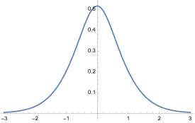
Note that, like the Cauchy distribution itself, this freely infinitely divisible law has a strictly positive density on all of . The law of (the Cauchy distribution) has no finite integer moments; nevertheless, it is the Lévy measure of the above freely infinitely divisible distribution, which has (exactly) two finite integer moments: is continuous and bounded, and .
Acknowledgments
The authors would like to thank Serban Belinschi and Ching Wei Ho for several very useful conversations clarifying core ideas of this work.
A few comments on the name ‘El Gordo’ (Lemma 3.4), which is Spanish for ‘The Fat One’. As shown in some examples, e.g. Example 3.3(b), the El Gordo transform tends to spread the support out. As we discussed at the beginning of Section 3.3, is a free probability analogue of where is a random variable independent from , and this operation also has the effect of spreading out . We could give other reasons why this name is sensible, but honestly we chose this name because the insight to introduce this and related transforms came to the authors over many excellent lunches at the incomparable Tacos El Gordo in Chula Vista, California.
References
- [1] S. T. Belinschi and H. Bercovici, Atoms and regularity for measures in a partially defined free convolution semigroup, Math. Z. 248 (2004), no. 4, 665–674. MR 2103535
- [2] H. Bercovici and D. Voiculescu, Superconvergence to the central limit and failure of the Cramér theorem for free random variables, Probab. Theory Related Fields 103 (1995), no. 2, 215–222. MR 1355057
- [3] Hari Bercovici and Vittorino Pata, Stable laws and domains of attraction in free probability theory, Ann. of Math. (2) 149 (1999), no. 3, 1023–1060, With an appendix by Philippe Biane. MR 1709310
- [4] Hari Bercovici and Dan Voiculescu, Free convolution of measures with unbounded support, Indiana University Mathematics Journal 42 (1993), no. 3, 733–773.
- [5] by same author, Regularity questions for free convolution, Nonselfadjoint operator algebras, operator theory, and related topics, Oper. Theory Adv. Appl., vol. 104, Birkhäuser, Basel, 1998, pp. 37–47. MR 1639647
- [6] Hari Bercovici and Dan-Virgil Voiculescu, Lévy-Hinčin type theorems for multiplicative and additive free convolution, Pacific journal of mathematics 153 (1992), no. 2, 217–248.
- [7] P Biane, Processes with free increments, Mathematische Zeitschrift 227 (1998), 143–174.
- [8] T Cacoullos and V Papathanasiou, Lower variance bounds and a new proof of the central limit theorem, Journal of multivariate analysis 43 (1992), no. 2, 173–184.
- [9] Guillaume Cébron, Max Fathi, and Tobias Mai, A note on existence of free Stein kernels, Proceedings of the American Mathematical Society 148 (2020), no. 4, 1583–1594.
- [10] Sourav Chatterjee, Stein’s method for concentration inequalities, Probab. Theory Related Fields 138 (2007), no. 8, 305–321.
- [11] by same author, Fluctuations of eigenvalues and second order poincaré inequalities, Probability Theory and Related Fields 143 (2009), no. 1-2, 1–40.
- [12] Sourav Chatterjee and Partha S Dey, Applications of Stein’s method for concentration inequalities, The Annals of Probability 38 (2010), no. 6, 2443–2485.
- [13] Louis HY Chen, Larry Goldstein, and Qi-Man Shao, Normal approximation by Stein’s method, Springer Science & Business Media, 2010.
- [14] Murat A Erdogdu, Lee H Dicker, and Mohsen Bayati, Scaled least squares estimator for GLMs in large-scale problems, Advances in Neural Information Processing Systems 29 (2016).
- [15] Max Fathi, Larry Goldstein, Gesine Reinert, and Adrien Saumard, Relaxing the Gaussian assumption in shrinkage and SURE in high dimension, arXiv preprint arXiv:2004.01378 (2020).
- [16] Max Fathi and Brent Nelson, Free Stein kernels and an improvement of the free logarithmic sobolev inequality, Advances in Mathematics 317 (2017), 193–223.
- [17] Subhankar Ghosh and Larry Goldstein, Concentration of measures via size-biased couplings, Probability Theory and Related fields 149 (2011), no. 1, 271–278.
- [18] Larry Goldstein and Gesine Reinert, Stein’s method and the zero bias transformation with application to simple random sampling, The Annals of Applied Probability 7 (1997), no. 4, 935–952.
- [19] by same author, Distributional transformations, orthogonal polynomials, and stein characterizations, Journal of Theoretical Probability 18 (2005), 237–260.
- [20] Larry Goldstein and Uwe Schmock, Probabilistic interpretation of a theorem of Kolmogorov using the zero bias transformation, preprint (2023+).
- [21] Larry Goldstein and Xiaohan Wei, Non-Gaussian observations in nonlinear compressed sensing via stein discrepancies, Information and Inference: A Journal of the IMA 8 (2019), no. 1, 125–159.
- [22] Tobias Johnson and Erol Peköz, Concentration inequalities from monotone couplings for graphs, walks, trees and branching processes, arXiv preprint arXiv:2108.02101 (2021).
- [23] Todd Kemp, Introduction to random matrix theory, unpublished, 2013.
- [24] Qiang Liu, Jason Lee, and Michael Jordan, A kernelized Stein discrepancy for goodness-of-fit tests, International conference on machine learning, PMLR, 2016, pp. 276–284.
- [25] Qiang Liu and Dilin Wang, Stein variational gradient descent: A general purpose Bayesian inference algorithm, Advances in Neural Information Processing Systems 29 (2016).
- [26] Hans Maassen, Addition of freely independent random variables, J. Funct. Anal. 106 (1992), no. 2, 409–438. MR 1165862
- [27] James A. Mingo and Roland Speicher, Free probability and random matrices, Fields Institute Monographs, vol. 35, Springer, New York; Fields Institute for Research in Mathematical Sciences, Toronto, ON, 2017. MR 3585560
- [28] Alexandru Nica and Roland Speicher, On the multiplication of free -tuples of noncommutative random variables, Amer. J. Math. 118 (1996), no. 4, 799–837. MR 1400060
- [29] by same author, Lectures on the combinatorics of free probability, London Mathematical Society Lecture Note Series, vol. 335, Cambridge University Press, Cambridge, 2006. MR 2266879
- [30] Evangelos A. Nikitopoulos, Noncommutative functions and Fréchet derivatives of operator functions, Expo. Math. 41 (2023), no. 1, 115–163. MR 4557276
- [31] Evangelos A. Nikitopoulos, Todd A. Kemp, and David A. Jekel, A martingale approach to noncommutative stochastic calculus, Preprint.
- [32] Charles Stein, A bound for the error in the normal approximation to the distribution of a sum of dependent random variables, Proceedings of the sixth Berkeley symposium on mathematical statistics and probability, volume 2: Probability theory, University of California Press, 1972, pp. 583–602.
- [33] Fred W Steutel, Preservation of infinite divisibility under mixing and related topics, (1971).
- [34] Dan Voiculescu, Addition of certain noncommuting random variables, J. Funct. Anal. 66 (1986), no. 3, 323–346. MR 839105
- [35] by same author, The analogues of entropy and of Fisher’s information measure in free probability theory. I, Comm. Math. Phys. 155 (1993), no. 1, 71–92. MR 1228526
- [36] Jiun-Chau Wang, Local limit theorems in free probability theory, Ann. Probab. 38 (2010), no. 4, 1492–1506. MR 2663634