Impenetrable Barriers in the Phase Space of a Particle Around a Kerr Rotating Black Hole

Abstract

We study the phase space of a particle in the gravitational field of a rotating black hole described by the Kerr metric from a geometrical perceptive. In particular, we show the construction of a multidimensional generalization of the unstable periodic orbits and their stable and unstable invariant manifolds that direct the dynamics in the phase space. Those stable and unstable invariant manifolds divide the phase space and are robust under perturbations. To visualize the multidimensional invariant sets under the flow in the phase space, we use a method based on the arclength of the trajectories in phase space.

1 Introduction

The rotating black holes are the result of collisions of non-colinear masses and are present in the centre of galaxies like our Milky Way. The study of the dynamics of particles and light around rotating black holes has been important to understanding diverse astronomical phenomena in the universe and detecting them [1, 2]. Recently observations and new techniques in data data analysis have made it possible to visualize a black hole using the images of the gas around it [3].

The Kerr metric describes the gravitational field in a neighbourhood of a rotating black hole [4]. The motion of a particle around a Kerr black hole is Liouville integrable [5, 6], its Hamiltonian has 4 independent integrals of motion: the Hamiltonian $H$, the energy of the particle $E$, the component of the angular momentum around the rotation axis of the black hole $L$, and $Q$ the Carter integral. Using these integrals is possible to study the system in detail. Recent analytical studies of the phase space of this system show: the bifurcations of the main families of periodic orbits [7], homoclinic orbits in the equatorial plane [8, 9], trajectories converging to photon sphere [11], the classification of some bounded trajectories using angle-action variables [10], the classification of radial motion [12], the spherical orbits [13, 14], and other bounded trajectories relevant for astrophysics [15, 16].

In this work, we take a geometric approach to study and visualize the phase space of the system. In particular, we consider invariant objects under the dynamics in the phase space that generalize the unstable hyperbolic periodic orbits and their stable and unstable invariant manifolds. Considering the hole phase space, we can construct impenetrable barriers to understand the complete dynamics.

The rotation of the black hole is characterized by a parameter $a\in[0,1]$ proportional to the angular momentum of the black hole. For $a=0$, the black hole is not rotating and its gravitational field is described by the Schwarzschild metric [17]. In this case, the spatial part of the metric is spherically symmetric, it is natural to construct an effective potential energy parameterized by the angular momentum $L$ to describe the radial motion of the particle. Associated with the maximum value of this effective potential energy, there is a family of unstable hyperbolic periodic orbits. Their stable and unstable manifolds of unstable hyperbolic periodic orbits play a fundamental role in the analysis of the phase space of the system. In particular, for the construction of the impenetrable barriers in the phase space in the non-integrable perturbed case.

Considering those geometrical properties of the system, we construct a Normally Hyperbolic Invariant Manifold (NHIM) taking the union of all unstable periodic orbits associated with the maximum of the effective potential for all the different directions on the sphere. The stable and unstable manifolds of this NHIM have coodimension one relative to the constant energy manifold. Therefore, they are impenetrable barriers that direct the dynamics.

An important property of the NHIMs and their stable and unstable invariant manifolds is that they are robust under generic perturbation of the Hamiltonian [18, 19, 20, 21, 22, 23, 24]. Then, the internal NHIM of the system and the impenetrable barriers in the phase space formed by their stable and unstable manifolds persist when the symmetries of the system are broken and the dynamics becomes chaotic.

The article is organized as follows: In section 2, we show the Hamiltonian function of the system in the Boyer-Lindquist coordinates and the integrals of motion of the system. The section 3, we construct the NHIM for the non-rotating black hole, $a=0$, using the effective potential obtained from the equation for the motion of the radial coordinate. Also, we show plots of the stable and unstable manifolds of the NHIM using the technique of Lagrangian descriptors constructed with the arclength of the trajectories in phase space [25, 26, 27, 28]. In section 4, we break the spatial spherical symmetry with the inclusion of the rotation of the black hole, $a>0$, and visualize the changes in the invariant manifolds. Finally, we present the conclusions and final remarks in the last section.

2 Hamiltonian Function and Integrals of Motion

A convenient set of coordinates to express the metric of the systems is the Boyer-Lindquist coordinates $r,\theta,\phi,t$ [29]. These coordinates simplify the expression of the Kerr metric and facilitate the analysis of the phase space of the system [2, 5, 7, 8, 9, 10]. In these coordinates, the interval has only one mixed term. The Kerr metric with natural units $G,c=1$, in the Boyer-Lindquist coordinates is given by

$$ds^{2}=-m^{2}d\tau^{2}= - \left(1-\frac{2Mr}{\Sigma}\right)dt^{2}-\frac{4Mar\sin^{2}\theta}{\Sigma}dtd\varphi$$

$$+ \frac{\Sigma}{\Delta}dr^{2}+\Sigma d\theta^{2}+\sin^{2}\theta\left(r^{2}+a^{2}+\frac{2Ma^{2}r\sin^{2}\theta}{\Sigma}\right)d\varphi^{2}\;,$$

where $\tau$ is the proper time of the particle, $m$ and $M$, are the mass of the particle and the black hole respectively, $a$ is the spin parameter and the functions $\Sigma$ and $\Delta$ are defined as

$$\Sigma(r,\theta) = r^{2}+a^{2}\cos^{2}\theta\;,$$

$$\Delta(r) = r^{2}-2Mr+a^{2}\;.$$ (2)

In order to simplify the notation, we use the convention $M=1$. From his metric is possible to calculate the Hamiltonian function of a particle around a rotating black hole. In particular, we are going to use the Hamiltonian function constructed in the reference [10]. The Hamiltonian function of the systems in Boyer-Lindquist coordinates is given by

$$H(r,\theta,\varphi,t,p_{r},p_{\theta},p_{\varphi},p_{t})=\frac{\Delta}{2\Sigma}p_{r}^{2}+\frac{1}{2\Sigma}p_{\theta}^{2}-\frac{R+\Delta\Theta}{2\Delta\Sigma}-\frac{1}{2}\;,$$ (3)

where the functions $\Theta$, $R$ are defined as

$$\Theta(\theta) = Q-\cos^{2}\theta\;\left\{a^{2}(1-E^{2})+\frac{L^{2}}{\sin^{2}\theta}\right\}\;,$$

$$R(r) = P^{2}-\Delta\left\{r^{2}+(L-aE)^{2}+Q\right\}\;,$$

$$P(r) = E(r^{2}+a^{2})-aL\;.\quad$$ (4)

The corresponding Hamilton’s equations of motion parametrized by the proper time $\tau$ of the particle are

$$\dot{r} = \frac{\Delta}{\Sigma}p_{r},$$

$$\dot{p}_{r} = \frac{\partial}{\partial r}\left(\frac{\Delta}{2\Sigma}\right)p^{2}_{r}-\frac{\partial}{\partial r}\left(\frac{1}{2\Sigma}\right)p^{2}_{\theta}+\frac{\partial}{\partial r}\left(\frac{R+\Delta\Theta}{2\Delta\Sigma}\right),$$

$$\dot{\theta} = \frac{1}{\Sigma}p_{\theta},$$

$$\dot{p}_{\theta} = \frac{\partial}{\partial\theta}\left(\frac{\Delta}{2\Sigma}\right)p^{2}_{r}-\frac{\partial}{\partial\theta}\left(\frac{1}{2\Sigma}\right)p^{2}_{\theta}+\frac{\partial}{\partial\theta}\left(\frac{R+\Delta\Theta}{2\Delta\Sigma}\right),$$

$$\dot{\phi} = -\frac{1}{2\Delta\Sigma}\frac{\partial}{\partial E}\left(R+\Delta\Theta\right),$$

$$\dot{p}_{\phi} = 0,$$

$$\dot{t} = -\frac{1}{2\Delta\Sigma}\frac{\partial}{\partial L}\left(R+\Delta\Theta\right),$$

$$\dot{p}_{t} = 0.$$ (5)

This Hamiltonian system is integrable, the system of differential equations has 4 independent integrals of motion: the value of the Hamiltonian $H$, the energy $E=-p_{t}$ of the particle, the angular momentum $L=p_{\varphi}$, and the Carter integral $Q$. The first 3 integrals are immediate to obtain from the structure of the Hamiltonian, however the last one, $Q$ was obtained by Carter in [5, 15] proposing a separation of variables of solution of the resulting Hamilton–Jacobi equation in other canonical coordinates. From that approach is possible to obtain the first-order geodesic equations in a natural way. Those differential equations in the Boyer-Lindquist coordinates are given by

$$m\Sigma\dot{r} = \pm\sqrt{R}\;,$$

$$m\Sigma\dot{\theta} = \pm\sqrt{\Theta}\;,$$

$$m\Sigma\dot{\varphi} = \frac{a}{\Delta}(2rE-aL)+\frac{L}{\sin{\theta}}\;,$$

$$m\Sigma\dot{t} = \frac{(r^{2}+a^{2})^{2}E-2arL}{\Delta}-a^{2}E\sin{\theta}\;.$$ (6)

This set of differential equations is very convenient for analysing the analytical important properties like bifurcations of the integrable system [7, 13, 15, 16]. However, for the numerical calculations in the present article, we are going to use Hamilton’s equations 5 like in works [8, 9, 10]. We use the equations of motion obtained directly from the Hamiltonian function 3 because we want to understand properties relevant to non-integrable cases, where all the equations of motion are coupled. Also from the numerical point of view the system 5 are easier to code because there are no change signs related to the square roots like in 6.

Also, we can construct the reduced 6-dimensional phase space to describe the dynamics of the system using the global time $t$ to parametrize the solutions of the systems of differential equations. To construct the system of differential equations for the reduced phase space, we only need to use the differential equation for $\dot{t}=\frac{dt}{d\tau}$ and the chain rule $\frac{d}{dt}=\frac{d\tau}{dt}\frac{d}{d\tau}$ to calculate the derivative whit respect to $t$ of the other coordinates and momenta in the system, for more details see the reference [9].

3 NHIM and its Stable and Unstable Manifolds for the Schwarzschild Black Hole, $a=0$

The symmetries of the system facilitate the understanding of its multidimensional phase space. In the present case, the symmetries allow us to see the basic elements that constitute the invariant manifolds under the dynamics. Some recent examples where is possible to find the Normally Hyperbolic Invariant Manifold (NHIM) and their invariant manifolds using this approach are in the works [22, 23, 32, 33, 26, 30, 31].

First, let us consider the simplest case, $a=0$, where the Kerr metric is reduced to the Schwarzschild metric. In this case, the system has spatial spherical symmetry it is easy to construct and visualize the generalization of the hyperbolic periodic orbit and their invariant stable and unstable manifolds. Without loss of generality, we set $Q=0$ that corresponds to the motion on the equatorial plane, $\theta=\pi/2$. It is equivalent to any other plane due to the spherical symmetry of the Schwarzschild metric. From the geodesic equation for the radial coordinate 6, we can obtain the conservation equation for the energy $E$.

$$\frac{\dot{r}^{2}}{2}+V_{eff}(r;L)=E_{eff}=\frac{E^{2}}{2}\;,$$ (7)

where

$$V_{eff}(r;L)=\frac{m^{2}}{2}-\frac{m}{r}+\frac{L^{2}}{2r^{2}}-\frac{L^{2}}{r^{3}}\;$$ (8)

is the effective potential parametrized by the conserved component of the angular momentum $L$ and $E$ is the total energy of the particle.

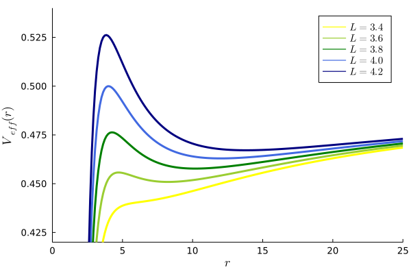
Figure 1: Effective potential $V_{eff}(r;L)$ for different values of $L$. As the value of $L$ is increased the maximum value of $V_{eff}(r;L)$ grows. Associated with each maximum there is an unstable hyperbolic fixed point $X_{L}$ in the phase space of the one-dimensional system with energy $E=E_{h}$. This fixed point is located at $X_{L}=(r=r_{L},p_{r}=0)$ where $r_{L}$ is the critical value of $V_{eff}(r;L)$.

Due to the existence of this effective potential $V_{e}ff(r;L)$ for the radial motion, let us consider the reduced phase space only for the radial degree of freedom. Associated with the maximum of the effective potential $V_{eff}(r;L)$ there is an unstable hyperbolic fixed point $X_{L}=(r=r_{L},p_{r}=0)$. There are two special sets in the phase space that divide the reduced 2-dimensional phase space in regions with different behaviour, the stable and unstable manifolds of the unstable hyperbolic fixed point denoted by $W^{s/u}(X_{h})$. The stable (unstable) manifold of the hyperbolic fixed point is the trajectory that converges (diverges) when the time is increased.

When we include the angular coordinate $\phi$ in the analysis of the dynamics, we have a 2-degree-of-freedom system. The unstable hyperbolic fixed point $X_{L}$ corresponds to a circular unstable hyperbolic periodic orbit $\gamma_{L}$ with radio $r_{L}$ in the configuration space. The unstable hyperbolic periodic orbit $\gamma_{L}$ also have stable and unstable manifolds $W^{s/u}(\gamma_{L})$. Those 2-dimensional invariant manifolds are formed by all the trajectories that converge (diverge) to $\gamma_{L}$ when the time to infinity. Also by construction, $W^{s/u}(\gamma_{L})$ divides the constant energy manifold of the 2-degree-of-freedom system.

Considering the spatial spherical symmetry of the system, we construct the generalization of this unstable hyperbolic periodic orbit in the constant energy manifold, the Normally Hyperbolic Invariant Manifold (NHIM) denoted as $\mathcal{M}_{E}$. Let us take the union of all the unstable circular periodic orbits with the energy $E$, associated with the maximum of $V_{eff}(r;L)$, for all the possible angular directions $\theta,\phi$ on the sphere in the configuration space.

$$\mathcal{M}_{E} = \bigcup_{\theta,\phi}\gamma_{L}=S^{2}\times\gamma_{L}$$ (9)

By construction, the topology of the NHIM $\mathcal{M}_{E}$ is a 3-dimensional sphere $S^{3}$. If we consider the degree of freedom corresponding to time $t$ in the construction of the NHIM, the result is a 4-dimensional unbounded NHIM given by $\mathcal{M}_{E}\times\mathbb{R}$.

Analogously, we construct the stable and unstable manifolds of the NHIM $\mathcal{M}_{E}$. Again, considering the spherical spacial symmetry of the system and taking the union of all the stable or unstable manifolds of $W^{s/u}(\gamma_{L})$ we obtain the invariant manifolds of the NHIM $\mathcal{M}_{E}$,

$$W^{s/u}(\mathcal{M}_{E}) = \bigcup_{\theta,\phi}W^{s/u}(\gamma_{L}).$$ (10)

By construction, the topology of $W^{s/u}(\mathcal{M}_{E})$ is a 4-dimensional spherical cylinder $S^{3}\times\mathbb{R}$. This spherical cylinder divides the 5-dimensional constant energy manifold in the reduced phase space that considers only the spatial degrees of freedom. Also, if we consider the degree of freedom corresponding to time $t$ in the construction of the invariant stable and unstable manifolds of the NHIM, the result is a 5-dimensional invariant manifold given by $W^{s/u}(\mathcal{M}_{E})\times\mathbb{R}$.

In order to visualize the invariant manifolds in multidimensional phase space, we calculate the scalar field of arclengths of the trajectories. The arclength of the trajectories is generated by their different behaviour give us information on the invariant manifolds that intersect the set of initial conditions where we calculate the scalar field. This scalar field is a type of Lagrangian descriptor scalar field. Some recent examples where the Lagrangian descriptors have been used to analyze the phase space of multidimensional systems are in [25, 26, 34, 35]. The basic definition of the Lagrangian descriptor based on arclength is in Appendix A and more illustrative examples are in the reference therein.

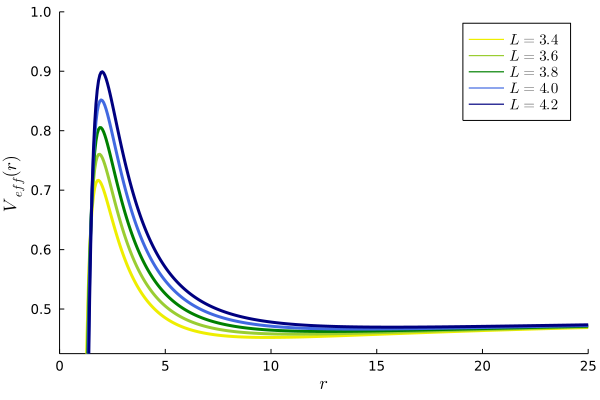
Figure 4: Effective potential $V_{eff}(r;a,E,L,Q)$ for different values of $a,E,L,Q$. Associated with each maximum there is an unstable hyperbolic fixed point in the phase space of the 1-dimensional system. This fixed point is located at $(r,p_{r})=(r_{(a,E,L,Q)},0)$ where $r_{(a,E,L,Q)}$ is the critical value of $V_{eff}(r;a,E,L,Q)$.

Let us consider some relevant values of $L$ where the phase space changes qualitatively. In this case, the changes in the phase space are related to changes in the geometry of the effective potential energy $V_{eff}(r;L)$. In Fig.4, we can see two important changes in the geometry of the effective potential energy $V_{eff}(r;L)$ as the value of $L$ is increased. The first important change in the effective potential $V_{eff}(r;L)$ is the collision between its maximum with its minimum at $L=L_{sc}=\sqrt{12}$. This collision generates a saddle-centre bifurcation in the phase space. To visualize the changes in the phase space, we calculate the Lagrangian descriptor for initial conditions in the canonical plane $r$–$p_{r}$ and two constant values of $L$, one slightly smaller than the critical value and the other slightly bigger, see Fig. 2 panels a) and b). We can see how the phase space grows abruptly and a bounded region appears. In Fig. 2 b), the boundaries of phase space are the intersection of invariant manifolds $W^{s/u}(\gamma_{L})$ with the set of initial conditions and the intersection point is the intersection with the unstable hyperbolic periodic orbit $\gamma_{L}$ .

The second important change in $V_{eff}(r;L)$ occurs when its maximum reach the asymptotic value $1/2$. For that value of $L=4$, the trajectories can escape to infinity and the phase space has a transition from bounded to unbounded. Analogously, we calculate the Lagrangian descriptor for initial conditions in the canonical plane $r$–$p_{r}$ and two constant values of $L$, one value slightly smaller than the critical value and other chosen value slightly bigger see Fig.2 panels c) and d). In Fig. 2 d), we can see the external branches of invariant manifolds $W^{s/u}(\gamma_{L})$ go to infinity.

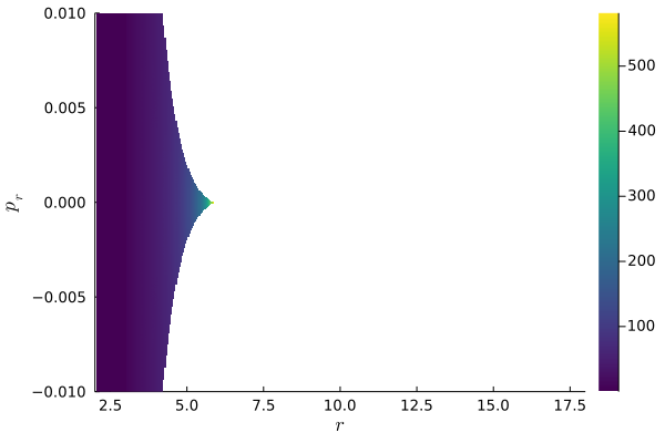
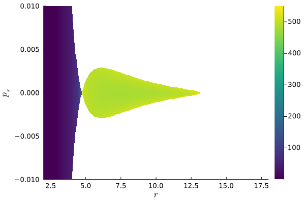
a) $L=3.4641<L_{sc}$	b) $L=3.6>L_{sc}$ , $E=E_{h}$
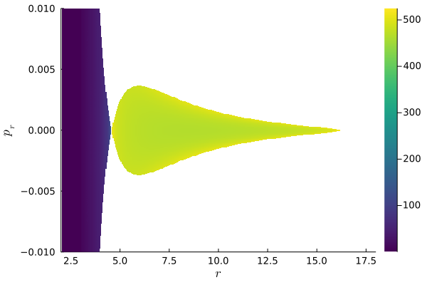
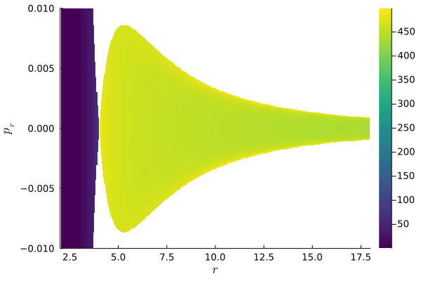
c) $L=3.65$, $E=E_{h}$	d) $L=4.0$, $E=E_{h}$

Figure 2: Lagrangian descriptor evaluated on the plane $r$–$p_{r}$ for different values of $E$, $L$, $p_{\theta}=0$, and $a=0$. The energy $E=E_{h}$ corresponds to the energy of the hyperbolic fixed point associated with the maximum of the effective potential $V_{e}ff(r;L)$.

Now, we consider the Lagrangian descriptor evaluated on initial conditions in the plane $r$–$p_{r}$ with the value of $E$ constant and the initial component of the momentum $p_{\theta}=0$. Let us remark that for these calculations the value of $L$ is determined by the other initial conditions and changes from point to point in the next plots. The Fig. 3 shows the results for 4 different values of $E$ or equivalently $E_{eff}$.

For $E_{eff}=0.44$, see Fig.3 a), the external branch of the stable manifold $W^{s}(\mathcal{M}_{E})$ and the external branch of unstable manifolds $W^{s/u}(\mathcal{M}_{E})$ coincide and divide the regions of the phase space with different behaviour. We can differentiate 3 regions: the yellow region corresponds to trajectories that are bounded, the dark blue region corresponds to trajectories that cross the event horizon and go inside the black hole, and the green region corresponds to trajectories that are unbounded and escape to infinity.

For $E_{eff}=0.45$, see Fig.3 b), we have a similar phase space structure with also 3 regions. However, the bounded yellow region does not reach the boundary of the domain of the Lagrangian descriptor plot. The intersection of the invariant manifolds of the NHIM $\mathcal{M}_{E}$ with the set of initial conditions form a closed curve that defines the boundary of the trapped region.

For $E_{eff}=0.49$, see Fig.3 c), shows that the trapped regions inside the separatrix formed by $W^{s/u}(\mathcal{M}_{E})$ disappear and the region that goes to the event horizon grows. The yellow-green regions correspond to regions with a large value of final $r$.

For $E_{eff}=0.51$, see Fig.3 d), the domain of the Lagrangian descriptor plot is unbounded, but the phase space with $r\in[0,30]$ has a similar structure like the panel c).

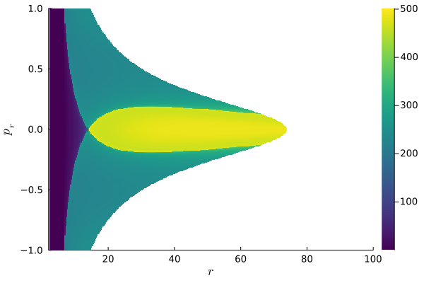
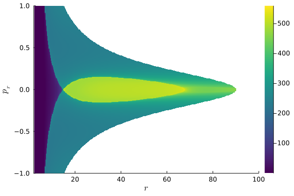
a) $E_{eff}=0.44$	b) $E_{eff}=0.45$
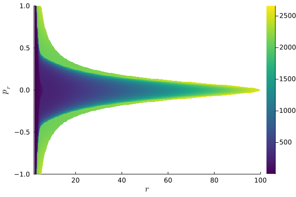
c) $E_{eff}=0.49$	d) $E_{eff}=0.51$

Figure 3: Lagrangian Descriptor evaluated on the plane $r$–$p_{r}$ for different values of $E$, and $a=0$.

4 NHIM and its Invariant Stable and Unstable Manifolds for Kerr Black Hole, $a>0$

For the rotating black hole, its angular momentum is non-zero, i.e $a>0$, the system lost its spatial spherical symmetry, however, it is still an integrable one [5]. A natural question is: What happens to the NHIM $\mathcal{M}_{E}$ and their stable and unstable manifolds $W^{s/u}(\mathcal{M}_{E})$? In general, the NHIMs and their stable and unstable manifolds are robust under perturbations of the vector field that define the system of ordinary differential equations [18, 21]. This fundamental geometrical property has been essential to understanding the dynamics in the multidimensional phase space for different systems where symmetry is broken, for example [32, 33, 26, 36, 37].

Let us denote the NHIM for $a>0$ as $\mathcal{M}_{E,a}$ and its stable and unstable invariant manifolds as $W^{s/u}(\mathcal{M}_{E,a})$. Recent works based on the integrability of the system and a change of variables [15, 13, 38] show analytical expressions for the trajectories contained in the NHIM $\mathcal{M}_{E,a}$ and their stable and unstable manifolds $W^{s/u}(\mathcal{M}_{E,a})$ for $a\in[0,1]$.

Moreover, we can understand the geometrical origin of the existence of the NHIM and its stable and unstable manifolds analogously than in the non-rotating case, $a=0$, considering again the equation 6 for the radial motion and the dynamical systems theory. In this case, the equation for the radial motion can be written as

$$\frac{m^{2}\Sigma^{2}}{r^{4}}\frac{\dot{r}^{2}}{2}+V_{eff}(r;a,E,L,Q)=E_{eff}=\frac{E^{2}}{2}\;,$$ (11)

where

$$V_{eff}(r;a,E,L,Q)=\frac{m^{2}}{2}-\frac{m}{r}+\frac{L^{2}-a^{2}(E^{2}-m^{2})+Q}{2r^{2}}-\frac{(L-aE)^{2}+Q}{r^{3}}+\frac{a^{2}Q}{2r^{4}}\;.$$ (12)

On the RHS of equation 11 we have the radial kinetic energy and the generalized effective potential energy $V_{eff}(r;a,E,L,Q)$. On the LHS of equation 11 we have a constant interpreted as the effective energy.

Let us notice that for $a=0$ and $Q=0$, the effective potential 12 and the radial equation of motion 11 are reduced to corresponding equations 8 and 7 in the previous section. Also, we obtain the same functional form for the effective potential with the change $L^{2}+Q\to L^{2}$ for the case $a=0$ and $Q\neq 0$. That represents the motion outside the equatorial plane in the non-rotational case. For more information about the bifurcation diagrams for all the parameters see the references [7, 13].

Let us remark that we can apply the theorem of persistence of NHIMs and their invariant manifolds to $\mathcal{M}_{E,a}$ and $W^{s/u}(\mathcal{M}_{E,a})$ for a perturbed Hamiltonian originated by a perturbed metric. Typically, the system becomes non-integrable and its dynamics is chaotic. Then the stable and stable manifolds $W^{s/u}(\mathcal{M}_{E,a})$ intersect transversally an infinite number of times and form a tangle in the phase space. This tangle is the multidimensional generalisation of the Smale horseshoes for the Poincare map of the 2-degree-of-freedom system, some examples are in the references [32, 36, 39, 35].

The next figures show changes in the phase space for different values of the effective energy of the particle $E_{eff}$ and different values of the rotation parameter $a$. In general, we can appreciate how the trapped region grows when the rotation of the black hole is increased.

For the effective energy $E_{eff}=0.44$, Fig. 5, the domain of the Lagrangian descriptor plot is bounded and the separatrix formed by the invariant manifolds $W^{s/u}(\mathcal{M}_{E,a})$. For $E_{eff}=0.45$, Fig. 6, the trapped region is bigger than in the previous case but the phase space structure is very similar. In Fig. 7, $E_{eff}=0.49$, the structure of the phase space changes, and the trapped region does not reach the maximum value of $r$ in the domain for moderate values of $a$. For $E_{eff}=0.51$, the phase space becomes unbounded, see Fig. 8. However, the trapped region has a similar behaviour to the previous case.

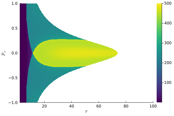
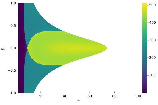
$a=0.1$	$a=0.2$
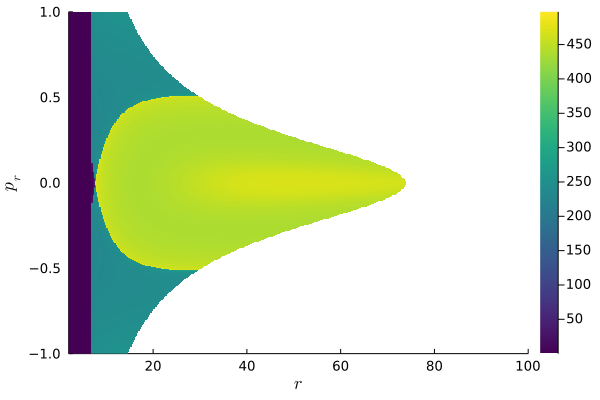
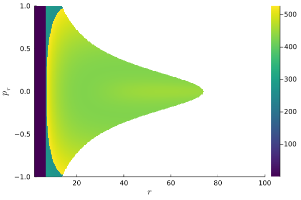
$a=0.3$	$a=1.0$

Figure 5: Lagrangian Descriptor evaluated on the plane $r$–$p_{r}$ for $E_{eff}=0.44$, different values of $a$.

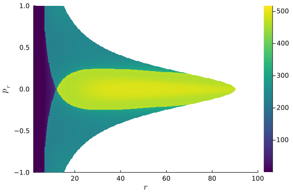
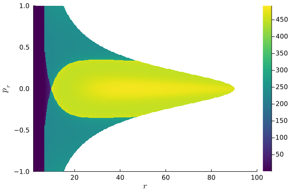
$a=0.1$	$a=0.2$
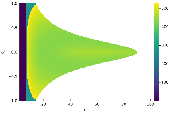
$a=0.3$	$a=1.0$

Figure 6: Lagrangian Descriptor evaluated on the plane $r$–$p_{r}$ for $E_{eff}=0.45$, different values of $a$.

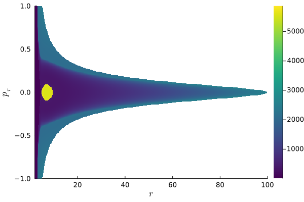
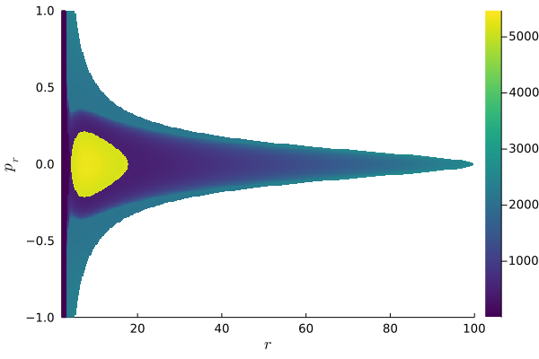
$a=0.1$	$a=0.2$
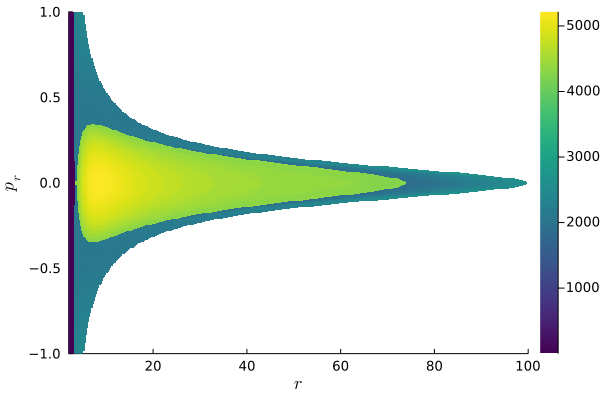
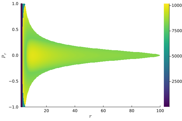
$a=0.3$	$a=1.0$

Figure 7: Lagrangian Descriptor evaluated on the plane $r$–$p_{r}$ for $E_{eff}=0.49$, different values of $a$.

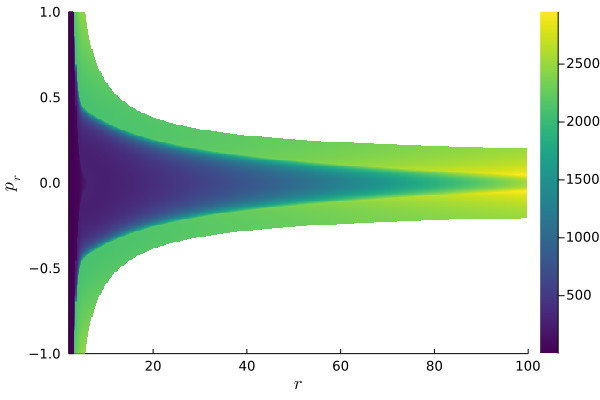
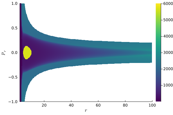
$a=0.1$	$a=0.2$
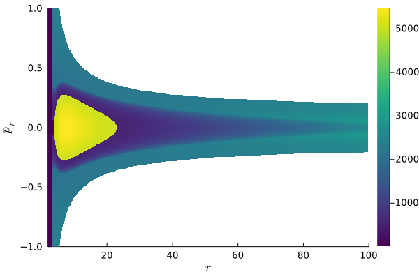
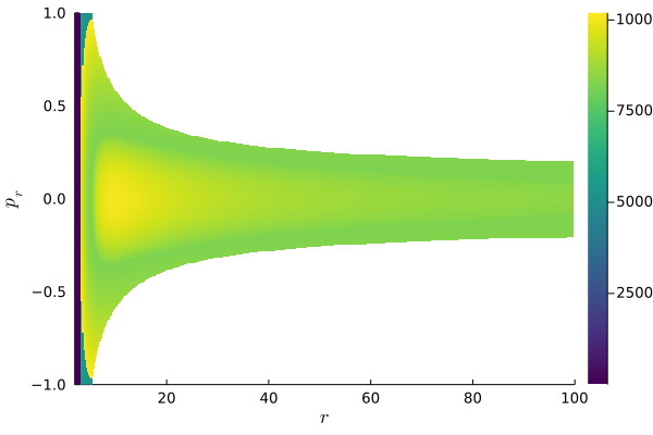
$a=0.3$	$a=1.0$

Figure 8: Lagrangian Descriptor evaluated on the plane $r$–$p_{r}$ for $E_{eff}=0.51$, different values of $a$.

5 Conclusions and Remarks

In this work, we study the phase space of a particle around a rotating Kerr black hole using the Boyer-Lindquist coordinates. The dynamics of this system is integrable and has 4 conserved quantities: the value of the Hamiltonian $H$, the energy $E=-p_{t}$ of the particle, the angular momentum $L=p_{\varphi}$, and the Carter integral $Q$. From the radial first integral equation is possible to construct an effective potential $V_{eff}(r;a,E,L,Q)$ parametrized by the rotation parameter of the black hole $a$ and the conserved quantities of the system. Using this radial effective potential, we construct a family of unstable periodic orbits associated with the maximum value of the effective potential for a fixed value of $E$. The union of those unstable hyperbolic periodic orbits form a Normally Hyperbolic Invariant Manifold (NHIM) $\mathcal{M}_{E,a}$ that has a central role in the dynamics in the reduced phase space.

The stable and unstable manifolds $W^{s/u}(\mathcal{M}_{E,a})$ have codimension one relative to the constant energy manifold and divide it into regions with different behaviour, see Figs.3,5,6,7,8. Due to the integrability of the system, one branch of the stable and unstable manifolds $W^{s/u}(\mathcal{M}_{E,a})$ coincide and form a separatrix that encircles the KAM tori associated with the minimal of the effective potential. The internal branches of $W^{s/u}(\mathcal{M}_{E,a})$ form an impenetrable barrier in the phase space that defines the set of trajectories that can cross the event horizon. In one way, the phase space of this system is similar to other multidimensional scattering systems [26, 32, 36, 39], but in this case the open branches of $W^{s/u}(\mathcal{M}_{E,a})$ go to the central region instead of the asymptotic region, $r\to\infty$.

We analyze the changes in the phase space of the system when the parameters change using Lagrangian descriptor plots. On those plots, we can see the intersections of the $W^{s/u}(\mathcal{M}_{E,a})$ with the set of initial conditions. In particular, we appreciate that when the rotation of the black hole grows the trapped region also grows. Therefore, when the angular moment of the black hole grows more it drags more of the particles around it.

An important difference between the cases $a>0$ and $a=0$ is that the NHIM constructed from the prograde orbits, $L>0$, and the NHIM constructed from the retrograde orbits, $L<0$, have different spatial projections because the effective potential energy $V_{e}ff(r;a,E,L,Q)$ is not symmetric respect the change $L\to-L$.

All the results for bounded NHIMs in the reduced phase space defined by the spatial degrees of freedom $r,\theta,\phi$ can be generalized to the case when we include the time $t$ as a degree of freedom. In this case, we need to consider the theory for unbounded NHIMs and their invariant stable and unstable manifolds developed in [24].

In future works, we are going to study the phase space of a perturbed Kerr Black hole. When the metric is perturbed, the symmetries are broken and the dynamics of the system becomes chaotic. However, the NHIMs and their stable and unstable invariant manifolds are robust under perturbations. This fundamental property allows us to analyse the perturbed chaotic systems. For a non-integrable perturbation, the stable and unstable manifolds of NHIM intersect transversely and form a rich structure analogous to the Smale horseshoes in more dimensions. The stable and unstable manifolds form a system of tubes that determine the transport in the phase space in the region close to the NHIM. Also, the internal dynamics of the NHIM becomes chaotic and give us information about the bifurcations of the NHIM.

Also, the NHIMs $\mathcal{M}_{E,a}$ define a dividing surface in the phase space like in Wiggner’s Transition State Theory for chemical reaction dynamics in phase space [40, 41, 42, 43]. Using this surface in the phase space is possible to calculate the total flux of trajectories that cross the saddle in potential energy and can reach the external event horizon.

6 Acknowledgments

This research was funded by DGAPA UNAM grant number AG–101122,
CONAHCyT CF–2023–G–763, and CONAHCyT fronteras grant number 425854. The author thanks the Virtual Institute of Physics at New York (VIP–NY), and Centro Internacional de Ciencias AC–UNAM for their facilities during the early stages of this work.

7 Appendix A: Lagrangian descriptors a tool to visualize the phase space

The Lagrangian descriptors are scalar fields to visualize invariant objects in the multidimensional phase space. The main idea behind the method is based on the different behaviour of the trajectories contained in different invariant objects in the phase space [25, 26, 27, 28]. Some recent illustrative examples of this phase space visualisation technique are in the references [44, 45, 46]. For instance, let us consider two trajectories with close initial conditions. One trajectory is contained in a stable manifold of an unstable periodic orbit $W^{s}(\gamma)$ and the other trajectory, with close initial conditions, but not contained in $W^{s}(\gamma)$. The trajectory that belongs to $W^{s}(\gamma)$ converges to $\gamma$, meanwhile the other trajectory is close only for a finite interval of time. This different behaviour generates a significant difference in the value of the scalar field.

A way to measure this different behaviour of the trajectories is the arclength of the trajectories for a given evolution time. The Lagrangian descriptor evaluated on the point $x_{0}$ in the phase space is defined as

$$LD[x(t)]=\int^{t_{f}}_{t_{i}}\sqrt{\sum_{j}(\dot{x}_{j}(t))^{2}}dt\;,$$ (13)

where $x(t)$ is the solution of the ODE system such that $x(t_{0})=x_{0}$, $\dot{x}_{j}$ are the components of the vector field that define the ODE system $\dot{x}=f(x)$, and $[t_{i},t_{f}]$ is the integration interval. In this example, if the particle reaches the exterior event horizon, we stop the integration.

8 Appendix B: Stability of Periodic Orbits on the NHIM and its relation with the Effective Potential

The NHIM $\mathcal{M}_{E}$ is constructed with the periodic orbits $\gamma_{L}$. Those periodic orbits and their stability on the radial direction are defined by the equations

$$\dot{r} = \pm\frac{\sqrt{R}}{m\Sigma}=0\;,$$ (14)

$$\frac{\partial\dot{r}}{\partial r} > 0\;.$$ (15)

Substituting the definitions of $R$ and $\Sigma$, we can find that previous equations are equivalent to

$$R = 0\;,$$ (16)

$$\frac{dR}{dr} = 0\;,$$ (17)

$$\frac{d^{2}R}{dr^{2}} > 0\;.$$ (18)

In terms of the effective potential energy, $V_{eff}$ those conditions are related to its local maximum given by

$$\frac{\partial V_{eff}}{\partial r} = 0\;,$$ (19)

$$\frac{\partial^{2}V_{eff}}{\partial r^{2}} < 0\;.$$ (20)

For more information about the parameter space and the bifurcation diagrams of the system, see the recent works [7, 13, 15, 16].

References

- [1] S. Chandrasekhar, The Mathematical Theory of Black Holes (Oxford: Clarendon Press, 1983)
- [2] D. L. Wiltshire, M. Visser, S. M. Scott, The Kerr Spacetime: Rotating Black Holes in General Relativity (Cambridge University Press, 2009)
- [3] The Event Horizon Telescope Collaboration et al, First M87 Event Horizon Telescope Results. IV, Imaging the Central Supermassive Black Hole, The Astrophysical Journal Letters. 875, 1, L1 (2019)
- [4] R. P. Kerr, Gravitational field of a spinning mass as an example of algebraically special metrics. Phys. Rev. Lett. 11, 237 (1963)
- [5] B. Carter, Global Structure of the Kerr Family of Gravitational Fields, Phys. Rev. 174, 1559 (1968)
- [6] B. Carter, Axisymmetric Black Hole Has Only Two Degrees of Freedom, Phys. Rev. 26, 331 (1971)
- [7] I. Bizyaev and I. Mamaev, Bifurcation diagram and a qualitative analysis of particle motion in a Kerr metric, Phys. Rev. D 105, 063003 (2022)
- [8] J. Levin and G. Perez-Giz, Homoclinic Orbits around Spinning Black Holes I: Exact Solution for the Kerr Separatrix. Phys. Rev. D 79, 124013 (2009)
- [9] J. Levin and G. Perez-Giz, Homoclinic Orbits around Spinning Black Holes II: The phase space portrait, Phys. Rev. D 79, 124014 (2009)
- [10] J. Levin and G. Perez-Giz, A periodic table for hole orbits, Phys. Rev. D 77, 103005 (2008)
- [11] A. Sneppen, Divergent reflections around the photon sphere of a black hole, Sci. Rep. 11, 14247 (2021).
- [12] G. Compère, Y Liu, J Long, Classification of radial Kerr geodesic motion, Phys. Rev. D 105, 024075 (2022)
- [13] E. Teo, Spherical orbits around a Kerr black hole. General Relativity and Gravitation, 53, 10 (2022)
- [14] E. Teo, Spherical photon orbits around a Kerr black hole. General Relativity and Gravitation 35, 1909 (2003)
- [15] P. Rana and A. Mangalam, Astrophysically relevant bound trajectories around a Kerr black hole. Classical and Quantum Gravity, 36, 045009 (2019)
- [16] P. Rana and A. Mangalam, Bound orbit domains in the phase space of the Kerr geometry, The Fifteenth Marcel Grossmann Meeting, 858 (2022)
- [17] R. Wald, General Relativity (Chicago, 1984)
- [18] N. Fenichel, Persistence and smoothness of invariant manifolds for flows, Indiana Univ. Math. J., 21, 193 (1971)
- [19] N. Fenichel, Asymptotic Stability With Rate Conditions. Indiana Univ. Math. J. 23, 12, 1109 (1974)
- [20] N. Fenichel, Asymptotic Stability with Rate Conditions II, Indiana Univ. Math. J. 26, 1, 81 (1977)
- [21] S. Wiggins, Normally Hyperbolic Invariant Manifolds in Dynamical Systems (Springer Verlag, Berlin 1994)
- [22] S. Wiggins, The role of normally hyperbolic invariant manifolds (NHIMS) in the context of the phase space setting for chemical reaction dynamics. Regul. Chaot. Dyn. 21, 621 (2016)
- [23] S. Wiggins, L. Wiesenfeld, C. Jaffé, and T. Uzer, Impenetrable Barriers in Phase-Space, Phys. Rev. Lett. 86, 5478 (2001)
- [24] J. Eldering, Normally Hyperbolic Invariant Manifolds. The noncompact case. ( Atlantis Press Paris, 2013 )
- [25] S. Wiggins and V. J. G. García-Garrido, Painting the Phase Portrait of a Dynamical System with the Computational Tool of Lagrangian Descriptors. Notices of the American Mathematical Society, 69, 936 (2022)
- [26] F. Gonzalez Montoya, The Classical Action as a Tool to visualize the Phase Space of Hamiltonian Systems, Dynamics, 4, 3 (2023)
- [27] A. M Mancho, S. Wiggins, J. Curbelo, C. Mendoza, Lagrangian Descriptors: A Method for Revealing Phase Space Structures of General Time Dependent Dynamical Systems. Commun. Nonlinear Sci. Numer. Simul., 18, 3530 (2013)
- [28] C. Lopesino, F. Balibrea-Iniesta, V. J. García-Garrido, S. Wiggins, A. M. Mancho, A Theoretical Framework for Lagrangian Descriptors, International Journal of Bifurcation and Chaos, 27, 1730001 (2017)
- [29] R. H. Boyer and R. W. Lindquist, Maximal Analytic Extension of the Kerr Metric, J. Math. Phys. 8, 265 (1967)
- [30] M. Firmbach, A. Bäcker, R. Ketzmerick, Partial barriers to chaotic transport in 4D symplectic maps, Chaos 33, 1 013125 (2023)
- [31] J. Stöber, Classical and quantum transport in 4d symplectic maps. Technische Universität Dresden, PhD tesis (2023)
- [32] F. Gonzalez Montoya and C. Jung, The numerical search for the internal dynamics of NHIMs and their pictorial representation, Physica D 436, 133330 (2022)
- [33] F. Gonzalez Montoya and C. Jung, Visualizing the perturbation of partial integrability, J. Phys. A: Math. Theor, 48 , 43 (2015)
- [34] F. Gonzalez Montoya and S. Wiggins, Phase space structure and escape time dynamics in a van der Waals model for exothermic reactions, Phys. Rev. E, 102 062203 (2020)
- [35] F. Gonzalez Montoya, F. Borondo, C. Jung, Atom scattering off a vibrating surface: an example of chaotic scattering with three degrees of freedom, Commun. Nonlinear Sci. Numer. Simul., 90, 105282 (2020)
- [36] G. Drotos, F. Gonzalez, C. Jung, The decay of a normally hyperbolic invariant manifold to dust in a three degrees of freedom scattering system, J. Phys. A: Math. Theor, 47, 045101 (2014)
- [37] G. Drótos, F. González Montoya, C. Jung, T. Tél, Asymptotic observability of low-dimensional powder chaos in a three-degrees-of-freedom scattering system, Phys. Rev. E, 90, 2, 22906 (2014)
- [38] L.C. Stein, N. Warburton, Location of the last stable orbit in Kerr spacetime. Phys. Rev. D, 101, 064007 (2020)
- [39] C. Jung, O. Merlo, T. H. Seligman and W. P. K. Zapfe, The chaotic set and the cross section for chaotic scattering in three degrees of freedom, New J. Phys. 12, 103021 (2010)
- [40] H. Waalkens, R. Schubert, S. Wiggins, Wigner’s dynamical transition state theory in phase space: classical and quantum, Nonlinearity, 21, R1 (2007)
- [41] M. Katsanikas, S. Wiggins, The Generalization of the Periodic Orbit Dividing Surface in Hamiltonian Systems with three or more degrees of freedom–I, International Journal of Bifurcation and Chaos, 31, 2130028 (2021)
- [42] M. Katsanikas, S. Wiggins, The Generalization of the Periodic Orbit Dividing Surface in Hamiltonian Systems with three or more degrees of freedom–II, International Journal of Bifurcation and Chaos, 31, 2150188 (2021)
- [43] M. Katsanikas, S. Wiggins, The Generalization of the Periodic Orbit Dividing Surface in Hamiltonian Systems with three or more degrees of freedom–III, International Journal of Bifurcation and Chaos, 33, 2350088 (2023)
- [44] R. Crossley, M. Agaoglou, M Katsanikas, S. Wiggins, From Poincaré Maps to Lagrangian Descriptors: The Case of the Valley Ridge Inflection Point Potential, Regul. Chaot. Dyn. 26, 2 (2021)
- [45] M. Hillebrand, S. Zimper, A. Ngapasare, M. Katsanikas, S. Wiggins, C. Skokos, Quantifying chaos using Lagrangian descriptors, Chaos, 32, 12 (2022)
- [46] S. Zimper, A. Ngapasare, M. Hillebrand, M. Katsanikas, S. Wiggins, C. Skokos, Performance of chaos diagnostics based on Lagrangian descriptors. Application to the 4D standard map, Physica D, 453 133833 (2022)