Online Feedback Optimization over Networks:
A Distributed Model-free Approach

Abstract

Online feedback optimization (OFO) enables optimal steady-state operations of a physical system by employing an iterative optimization algorithm as a dynamic feedback controller. When the plant consists of several interconnected sub-systems, centralized implementations become impractical due to the heavy computational burden and the need to pre-compute system-wide sensitivities, which may not be easily accessible in practice. Motivated by these challenges, we develop a fully distributed model-free OFO controller, featuring consensus-based tracking of the global objective value and local iterative (projected) updates that use stochastic gradient estimates. We characterize how the closed-loop performance depends on the size of the network, the number of iterations, and the level of accuracy of consensus. Numerical simulations on a voltage control problem in a direct current power grid corroborate the theoretical findings.

I Introduction

Optimal steady-state operations of dynamical systems are a frequent and important engineering task, with examples from power grids, traffic networks, to mobile robot swarms. These systems are inherently complex, preventing us from constructing accurate models of their behaviors. Moreover, exogenous disturbances that act on systems are unknown in general, which adds to the difficulty of formulating explicit input-output maps. Therefore, computing optimal steady-state control inputs offline via numerical solvers and then applying them to the system in a feedforward manner is often suboptimal, lacking real-time adaptability and efficiency.

Online feedback optimization (OFO) [1, 2, 3] is an emerging control paradigm to steer complex dynamical systems to optimal steady-state operating points. Its core principle is to interconnect optimization algorithms in closed loop with a physical plant, thus circumventing the need for an explicit model of the plant and the exact value of the disturbance. OFO enjoys closed-loop optimality and stability in various scenarios, e.g., convex [4, 5, 6] and non-convex problems [7, 8, 9] with input[10] and output constraints[11], as well as linear [12, 13] and non-linear dynamical systems[6]. The effectiveness of OFO has been empirically demonstrated in real-world power distribution grids[14].

The above OFO controllers are mostly centralized. When applied to large-scale networked systems involving interconnected subsystems, they can face issues of scalability, robustness, privacy disclosure, that are common in large-scale centralized decision architectures [15]. First, a central processor is needed to communicate with all the subsystems and generate network-wide control inputs. Thus, there exist severe computational and communication bottlenecks for sizable networks. Second, this centralized architecture is not robust against potential failures or attacks at the central unit. Finally, since gradient-based OFO controllers (e.g., [10, 11, 1, 7]) require the system-wide input-output sensitivity to perform local iterative updates, concerns on privacy disclosure and challenges of local modeling also arise.

To tackle the issues of the centralized paradigm, multiple decentralized or distributed OFO controllers have been developed. Some decentralized methods[16, 8, 17] leverage local decision-making without inter-agent communication. While these methods ensure convergence to competitive equilibria (e.g., Nash), they experience sub-optimality compared to the globally optimal solutions. Other distributed approaches exploit consensus-based information exchange for coordination among neighbors [18, 19, 20]. The aforementioned controllers all use first-order iterations, and, therefore, still require local input-output sensitivities of agents. In terms of large-scale complex systems, the estimation of those local sensitivities can be highly non-trivial, prone to errors, or prohibitive due to lack of measurements, nonlinearity, and non-smoothness of input-output maps. To address unknown sensitivities, another line of works [9, 21, 22, 23] explore model-free OFO via stochastic gradient estimates developed in zeroth-order optimization [24, 25, 26]. Nonetheless, how to extend these centralized model-free methods to achieve distributed decision-making remains unclear.

In this paper, we propose a distributed model-free OFO controller to optimize the steady-state performance of a networked nonlinear system. To circumvent local sensitivities and satisfy input constraints, we leverage local iterative updates based on gradient estimates and projection. More importantly, to achieve fully distributed operations, we design a new protocol for maintaining and updating a queue of historical local objective values, which facilitates each agent to locally track the global objective value and construct gradient estimates. Our work is aligned with [27] that pursues cooperative optimization over networks. In contrast, we consider the input-output coupling between agents through dynamics and attain lower costs of local communication and storage, because we do not require a table that records the information of all the agents as [27]. We characterize the optimality of the closed-loop interconnection between the proposed controller and the networked system. Specifically, we quantify the distance to the optimal point as a function of the size of the network, the number of iterations, and the accuracy of consensus. We further apply the proposed distributed controller to a voltage control problem for a direct current power system.

II Problem Formulation and Preliminaries

Consider a networked system consisting of $N$ subsystems, or agents. The system is described by a graph $\mathcal{G}(\mathcal{N},\mathcal{E})$, where $\mathcal{N}$ and $\mathcal{E}\subseteq\mathcal{N}\times\mathcal{N}$ denote the set of agents and the set of edges, respectively. Agent $i$ can communicate with agent $j$ if and only if $(i,j)\in\mathcal{E}$, where $i,j\in\mathcal{N}$. The neighborhood of agent $i$ is represented by $\mathcal{N}_{i}$. Given a vector $w\in\mathbb{R}^{N}$, $w_{k}$ denotes its value at the $k$-th iteration, while $w(i)$ represents its $i$-th element.

II-A Problem Formulation

We consider a fast stable networked system described by its steady-state nonlinear algebraic map $h:\mathbb{R}^{N}\times\mathbb{R}^{N}\rightarrow\mathbb{R}^{N}$

$$y=h(u,d),$$ (1)

where $u\in\mathbb{R}^{N}$ is the input, $y\in\mathbb{R}^{N}$ is the output, and $d\in\mathbb{R}^{N}$ is an unknown exogenous disturbance. The $i$-th elements of $u$, $y$, and $d$ are the local input, output, and disturbance of agent $i$, respectively, where $i=1,\ldots,N$. In general, the map (1) represents the steady-state input-output map of a nonlinear system with coupled dynamics between agents as follows

$$\begin{split}x_{k+1}&=f(x_{k},u,d),\\ y_{k}&=g(x_{k},u,d),\end{split}$$ (2)

where $x_{k}\in\mathbb{R}^{N}$ is the state, and $f$ and $g$ are functions in the dynamics equations. We focus on a per-agent scalar setting to simplify notation, however, our results readily extend to scenarios involving multiple variables.

We aim to optimize the steady-state input-output performance of the networked system (1), i.e.,

$$\min_{u\in\mathbb{R}^{N},y\in\mathbb{R}^{N}}\quad \Phi(u,y)\triangleq\frac{1}{N}\sum_{i=1}^{N}\Phi_{i}(u(i),y(i))$$ (3a)

s.t. $$y=h(u,d),$$ (3b)

$$u\in\mathcal{U}\triangleq{\textstyle\prod_{i=1}^{N}}\mathcal{U}_{i}.$$ (3c)

In problem (3), the global objective function $\Phi:\mathbb{R}^{N}\times\mathbb{R}^{N}\rightarrow\mathbb{R}$ is the average of all the local objectives $\Phi_{i}:\mathbb{R}\times\mathbb{R}\rightarrow\mathbb{R}$, and $u(i)$ and $y(i)$ are the input and output of agent $i$, respectively. Moreover, $\mathcal{U}_{i}\subseteq\mathbb{R}$ is the local input constraint set of agent $i$. The overall constraint set $\mathcal{U}$ is the Cartesian product of all the local sets. By incorporating (3b) into the objective $\Phi$, problem (3) can be transformed to:

$$\begin{split}\min_{u\in\mathbb{R}^{N}}\quad&\tilde{\Phi}(u)\\ \text{s.t.}\quad&u\in\mathcal{U},\end{split}$$ (4)

where $\tilde{\Phi}(u)=\frac{1}{N}\sum_{i=1}^{N}\tilde{\Phi}_{i}(u)$, and $\tilde{\Phi}_{i}(u)\triangleq\Phi_{i}(u(i),y(i))$ is the reduced local objective. The disturbance $d$ becomes an unknown parameter in $\tilde{\Phi}(u)$. We make the following assumptions on the objectives and the network.

Assumption 1.

The reduced objective $\tilde{\Phi}_{i}$ of agent $i$ is $L_{0}$-Lipschitz, $L_{1}$-smooth, and $m$-strongly convex.

Assumption 2.

The graph $\mathcal{G}$ describing the networked system (1) is undirected and connected.

Both Assumptions 1 and 2 are standard in the literature of network control, see [28, 29, 27] and [15, 30], respectively.

Solving problem (3) with numerical optimization algorithms requires accurate knowledge of the static model $h$ and the disturbance $d$, which can be impractical in real-world applications [1]. In contrast, in this paper we aim to develop a fully-distributed OFO controller that leverages real-time output measurements $y$ to bypass the need for any model information related to the input-output map $h$.

II-B Gradient Estimation

The key technique that enables model-free operations is zeroth-order optimization, where a gradient estimate, constructed based on objective values and random exploration vectors, is used in the iterative update. In this paper, we utilize the one-point residual feedback estimate proposed in [25]. This scheme proposes to estimate the gradient of a generic cost function $\zeta:\mathbb{R}^{N}\rightarrow\mathbb{R}$, evaluated at $u_{k}$, using

$$\tilde{\nabla}\zeta(u_{k})=\frac{\zeta(u_{k}+\delta v_{k})-\zeta(u_{k-1}+\delta v_{k-1})}{\delta}v_{k},$$ (5)

where $u_{k},u_{k-1}\in\mathbb{R}^{N}$ are optimization variables, $\tilde{\nabla}\zeta(u_{k})$ is the gradient estimate, $\delta>0$ is the so-called smoothing parameter, and $v_{k},v_{k-1}$ are independent and identically distributed random vectors sampled from a multivariate normal distribution. The expectation of (5) equals the gradient of the smooth approximation $\zeta_{\delta}$ of $\zeta$, where $\zeta_{\delta}(u):=\mathbb{E}_{v\sim\mathcal{N}(0,I)}[\zeta(u+\delta v)]$, and $I\in\mathbb{R}^{N\times N}$ is the identity matrix. If $\zeta$ is convex and $L$ smooth, then $\zeta_{\delta}$ is also convex and $L$ smooth. Moreover, the smooth approximation $\zeta_{\delta}$ can be bounded as $\zeta(u)\leq\zeta_{\delta}(u)\leq\zeta(u)+\frac{L}{2}\delta^{2}N,\forall u\in\mathbb{R}^{N}$.

III Design of Distributed Model-free OFO Controllers

The centralized model-free OFO [9, 22, 23] for solving (4) requires a central processor to collect local objective values $\tilde{\Phi}_{i}(u)$, evaluate the global objective to construct a gradient estimate via (5), and then broadcast the updated solution. In practice, however, this centralized design faces challenges related to scalability, robustness, and privacy preservation[15].

In contrast, we pursue an OFO controller to regulate the system (1) in a distributed and collaborative manner. This controller employs a novel communication protocol, where each agent stores and exchanges a vector of historical evaluations of local objectives to track the global objective value. This vector is updated via average consensus in the same time scale as the local optimization iterations. In the remainder of this paper, we treat the unconstrained case of (4) (i.e., $\mathcal{U}=\mathbb{R}^{N}$) separately, to derive sharper results.

III-A Unconstrained Setting

We first consider problem (4) in the unconstrained scenario, i.e., $\mathcal{U}=\mathbb{R}^{N}$. The key idea of the proposed distributed OFO controller is to exchange and update local estimates of the global objective values, construct gradient estimates similar to (5), and then iteratively adjust local control inputs.

Algorithm 1 Model-free distributed OFO controller

0:  consensus parameter $\tau$, step size $\eta$, smoothing parameter $\delta$, $u_{0}\in\mathbb{R}^{N}$, initial vector $z_{i,0}\in\mathbb{R}^{\tau}$ of each agent, total number of iterations $T$

1:  for $k=0,\ldots,T-1$ do

2:     for every agent $i$ do

3:        evaluate $\tilde{\Phi}_{i}(u_{k}+\delta v_{k})=\Phi_{i}(u_{k}(i)+\delta v_{k}(i),y_{k}(i))$;

4:        $z_{i,k}(l)=\sum_{j\in\mathcal{N}_{i}}W_{ij}\bm{z}_{j,k}(l)$, $\forall l=1,\ldots,\tau$;

5:        $z^{(1)}_{i,k}=[z^{\top}_{i,k},\tilde{\Phi}_{i}(u_{k}+\delta v_{k})]^{\top}$;

6:        $u_{k+1}(i)=u_{k}(i)-\eta\frac{\Delta_{k}(i)}{\delta}$, where

$$\Delta_{k}(i)\!=\!\begin{cases}\bm{z}^{(1)}_{i,k}(1)v^{\text{init}}_{0}(i)&\text{if $k\!=\!0$},\\ (\bm{z}^{(1)}_{i,k}(1)\!-\!\bm{z}^{(1)}_{i,k-1}(1))v^{\text{init}}_{k}(i)&\text{if $0\!<\!k\!<\!\tau$},\\ (\bm{z}^{(1)}_{i,k}(1)\!-\!\bm{z}^{(1)}_{i,k-1}(1))v_{k-\tau}(i)&\text{if $k\!\geq\!\tau$};\end{cases}$$ (6)

7:        $z_{i,k+1}=[z^{(1)}_{i,k}(2),\ldots,z^{(1)}_{i,k}(\tau+1)]^{\top}$;

8:     end for

9:  end for

9:  $u_{T}$

The model-free distributed controller requires a suitable initialization of $\bm{z}_{i,0}\in\mathbb{R}^{\tau}$, where $\tau\in\mathbb{N}$ is a design parameter. Agent $i$ can evaluate the local objective $\tau$ times using $v^{\text{init}}_{l}(i)\sim\mathcal{N}(0,1)$ for $l=0,\ldots,\tau-1$ and stack the result in $\bm{z}_{i,0}$. Consequently, we have

$$\bm{z}_{i,0}=\Big{[}\tilde{\Phi}_{i}(u_{0}+\delta v^{\text{init}}_{0}),\ldots,\tilde{\Phi}_{i}(u_{0}+\delta v^{\text{init}}_{\tau-1})\Big{]}^{\top}.$$

We summarize the detailed steps of the proposed distributed OFO controller in Algorithm 1. At every iteration $k$, each agent $i$ generates a random exploration signal $v_{k}(i)\sim\mathcal{N}(0,1)$ synchronously and evaluates its local objective value $\tilde{\Phi}_{i}(u_{k}+\delta v_{k})=\Phi_{i}(u_{k}(i)+\delta v_{k}(i),y_{k}(i))$ with its local input $u_{k}(i)+\delta v_{k}(i)$ and local measured output $y_{k}(i)$, which captures the collective effect of the coupled dynamics. These local objective values are stored in a vector $\bm{z}_{i,k}\in\mathbb{R}^{\tau}$ of size $\tau$. Then, the agents update $\bm{z}_{i,k}$ via the average consensus step (see line 4 in Algorithm 1), where $W$ is a doubly stochastic matrix with Metropolis weights[15]. Afterward, the new local evaluation of $\tilde{\Phi}_{i}$ queues into $\bm{z}^{(1)}_{i,k}$, and the first element of $\bm{z}^{(1)}_{i,k}$ is taken out to facilitate the optimization iterations (see lines 6-7 in Algorithm 1). We illustrate the process of communicating and updating $\bm{z}_{i,k}$ in Fig. 1.

In fact, when $k\geq\tau+1$, the first element of $\bm{z}^{(1)}_{i,k}$ corresponds to performing $\tau$ consensus iterations for the local objective values at time $k\!-\!\tau$. This element closely approximates the global objective value at time $k\!-\!\tau$ with a suitable $\tau$, because $\bm{z}^{(1)}_{i,k}(1)$ equals $\sum_{j=1}^{N}W^{\tau}_{ij}\tilde{\Phi}_{j}(u_{k-\tau}+\delta v_{k-\tau})$.

Let $\bm{Z}_{k}\in\mathbb{R}^{(\tau+1)\times N}$ be the matrix whose $i$-th column is $\bm{z}^{(1)}_{i,k}$. We denote the first row of $\bm{Z}_{k}$ by $\bm{Z}_{k}(1)\in\mathbb{R}^{N}$. For $k\geq\tau+1$, the update for all the agents can be compactly written as

$$u_{k+1}=u_{k}-\eta\frac{1}{\delta}\big{(}\underbrace{\bm{Z}_{k}(1)^{\top}}_{W^{\tau}\varphi_{k\!-\!\tau}}-\underbrace{\bm{Z}_{k-1}(1)^{\top}}_{W^{\tau}\varphi_{k\!-\!\tau\!-\!1}}\big{)}\odot v_{k-\tau},$$ (7)

where $\varphi_{k-\tau}=[\tilde{\Phi}_{1}(u_{k-\tau}+\delta v_{k-\tau}),\ldots,\tilde{\Phi}_{N}(u_{k-\tau}+\delta v_{k-\tau})]^{\top}$ is of size $N$, and $x\odot y$ represents the Hadamard product between two vectors $x$ and $y$.

Remark 1.

The parameter $\tau$ regulates the trade-off between the accuracy of the gradient estimate and the communication burden. On the one hand, if $\tau$ is large, then $W^{\tau}$ approximates $\frac{1}{N}\mathbf{1}\mathbf{1}^{\top}$ well, where $\mathbf{1}\in\mathbb{R}^{N}$ is an all-ones vector. Thus, the distributed update (7) owns a comparable accuracy guarantee as that of its centralized counterpart. On the other hand, a large $\tau$ indicates an increased amount of data exchanged between neighboring agents at each iteration. In practice, we can choose $\tau$ according to the bandwidth of the communication channel and the specified accuracy requirement.

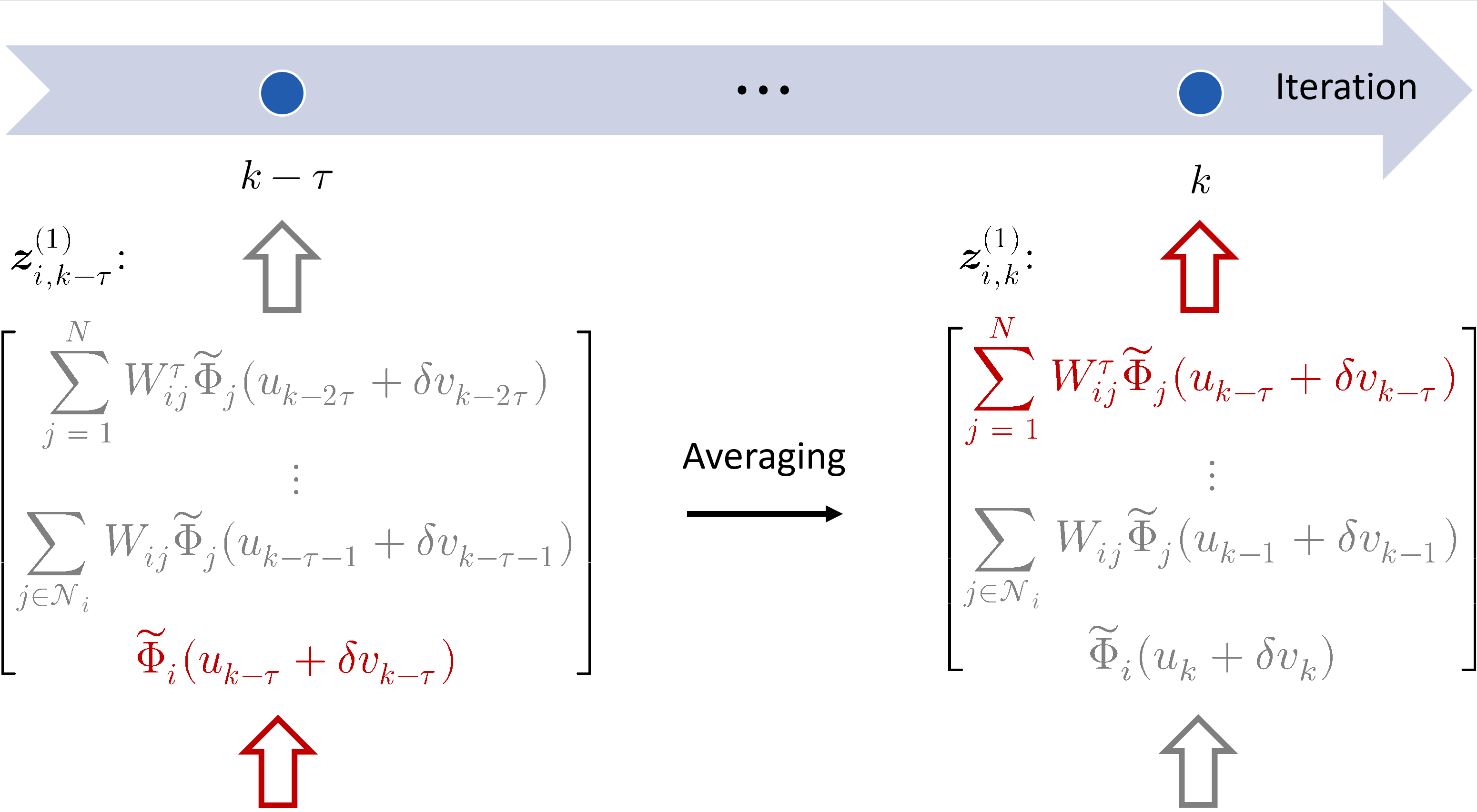
Figure 1: Illustration of the communication protocol.

III-B Constrained Setting

In many applications, there exist constraints on the admissible input. Such constraints can arise, for instance, from the upper and lower bounds imposed by actuation limits. We make the following assumption on the local input constraint set $\mathcal{U}_{i}$, where $i=1,\ldots,N$.

Assumption 3.

The set $\mathcal{U}_{i}\subseteq\mathbb{R}$ is convex, closed, and bounded with a diameter $D_{i}$, i.e., $\forall u,u^{\prime}\in\mathcal{U}_{i},|u-u^{\prime}|\leq D_{i}$.

Assumption 3 is commonly used in the literature, e.g., [27, 7, 31], and satisfied in applications. It implies the overall constraint set $\mathcal{U}=\prod_{i=1}^{N}\mathcal{U}_{i}$ is bounded by $D_{\mathcal{U}}\triangleq\sqrt{\sum_{i=1}^{N}D_{i}^{2}}$.

To handle the input constraint, we extend the proposed distributed controller (7) with projection. Namely, every agent $i$ performs the following update:

$$u_{k+1}(i)=\text{Proj}_{\mathcal{U}_{i}}\Big{[}u_{k}(i)-\frac{\eta}{\delta}\Delta_{k}(i)\Big{]},$$ (8)

where $\text{Proj}_{\mathcal{U}_{i}}[\cdot]$ denotes the projection onto $\mathcal{U}_{i}$, and $\Delta_{k}$ is as in (6).

IV Performance Guarantees

We provide convergence guarantees when the proposed distributed model-free controller (7) is implemented in closed loop with the system (1). We use the expected distance to the unique solution $u^{*}$ to problem (4), i.e., $\mathbb{E}[\|u_{k}-u^{*}\|^{2}]$, as the convergence measure. This metric is common in the literature when the objective is strongly convex and smooth [27, 15].

IV-A Unconstrained Setting

We first focus on the unconstrained scenario of problem (4), with $\mathcal{U}=\mathbb{R}^{N}$. Let the centralized gradient estimate as per (5) and the consensus error be defined by

$$\tilde{\nabla}\tilde{\Phi}(u_{k-\tau})=\frac{1}{\delta}\frac{1}{N}\mathbf{1}\mathbf{1}^{\top}(\varphi_{k-\tau}-\varphi_{k-\tau-1})\odot v_{k-\tau},$$

$$e_{k-\tau}=\frac{1}{\delta}(W^{\tau}-\frac{1}{N}\mathbf{1}\mathbf{1}^{\top})(\varphi_{k-\tau}-\varphi_{k-\tau-1})\odot v_{k-\tau}.$$

Therefore, the overall update (7) can be transformed to

$$u_{k+1}=u_{k}-\eta(\tilde{\nabla}\tilde{\Phi}(u_{k-\tau})+e_{k-\tau}),$$ (9)

where $e_{k-\tau}$ represents the error relative to the centralized gradient estimate arising from a finite number of consensus iterations. We further provide upper bounds on the second moments of gradient estimates and errors.

Lemma 1.

Let Assumptions 1 and 2 hold and $\mathcal{U}=\mathbb{R}^{N}$. If $0<\eta<\frac{\delta}{\sqrt{4NL_{0}^{2}\text{tr}(W^{2\tau})}}$, then for any $k>1$, $\mathbb{E}[\|\tilde{\nabla}\tilde{\Phi}(u_{k})+e_{k}\|^{2}]$, $\mathbb{E}[\|\tilde{\nabla}\tilde{\Phi}(u_{k})\|^{2}]$, and $\mathbb{E}[\|e_{k}\|^{2}]$ are bounded from above by $R$, $R_{f}$, and $R_{e}$, respectively, where $R$, $R_{f}$, and $R_{e}$ are constants give by

$$\begin{split}R=&\frac{1}{\alpha}\mathbb{E}[\|\tilde{\nabla}\tilde{\Phi}(u_{0})+e_{0}\|^{2}]+16L_{0}^{2}\text{tr}[W^{2\tau}](N+4)^{2}\frac{1}{1-\alpha},\\ R_{f}=&\frac{\alpha R}{2\text{tr}[W^{2\tau}]}+8L_{0}^{2}(N+4)^{2},\\ R_{e}=&\text{tr}[(W^{\tau}-\frac{1}{N}\mathbf{1}\mathbf{1}^{\top})^{2}]R_{f},\\ \end{split}$$

and the constant $\alpha=\frac{4N}{\delta^{2}}L_{0}^{2}\eta^{2}\text{tr}[W^{2\tau}]$.

Proof.

The proof can be found in Appendix -B. ∎

Note that $R_{e}$ exhibits a polynomial dependence on the number of agents $N$. Furthermore, the term $\text{tr}[(W^{\tau}-\frac{1}{N}\mathbf{1}\mathbf{1}^{\top})^{2}]$ describes how the consensus error decreases when $\tau$ increases. For $\eta$ and $\delta$ satisfying the conditions of Lemma 1, we can choose $\tau$ such that the error related to $e_{k}$ is arbitrarily small.

Next, we characterize the optimality of the closed-loop interconnection of the proposed controller (7) and system (1).

Theorem 1.

Given Assumptions 1 and 2, if $\mathcal{U}=\mathbb{R}^{N}$, $m>1$, and $0<\eta<\frac{\delta}{\sqrt{4NL_{0}^{2}\text{tr}(W^{2\tau})}}$, then for any $k\geq\tau+1$, the closed-loop system satisfies

$$\mathbb{E}[\|u_{k+1}-u^{*}\|^{2}]\leq\rho^{k-\tau}\mathbb{E}[\|u_{\tau+1}-u^{*}\|^{2}]+\frac{p(\eta)}{1-\rho},$$ (10)

where $\rho=1-(m-1)\eta+m\eta^{2}$, $p(\eta)=a_{1}\eta^{3}+a_{2}\eta^{2}+a_{3}\eta$, and $a_{1},a_{2},a_{3}$ are constants given by (15) in Appendix -C.

Proof.

The proof can be found in Appendix -C. ∎

Remark 2.

Theorem 1 requires that the strong convexity coefficient of $\tilde{\Phi}_{i}$ satisfies $m>1$. For those objectives that do not meet this requirement, we can scale them by some proper constants bigger than $1$, so that this condition is satisfied and the optimal point remains unchanged.

The upper bound (10) suggests that the influence of the transient distance to optimality $\mathbb{E}[\|u_{\tau+1}-u^{*}\|^{2}]$ vanishes exponentially fast. The error bound in the limit (i.e., $p(\eta)/(1-\rho)$) results from the bias of gradient estimates and the consensus errors. We further show that the limiting error bound can be made arbitrarily small by tuning $\tau$.

Corollary 1.

Consider a sufficiently small $\epsilon>0$. Let

$$\eta_{\epsilon} =(\sqrt{(a_{2}\!+\!0.5\epsilon m)^{2}\!+\!(2a_{1}\!+\!32N^{2}L_{1}L_{0}^{2}\text{tr}(W^{2\tau}))(m\!-\!1)\epsilon}$$

$$\quad-(a_{2}\!+\!0.5m\epsilon))/(2a_{1}\!+\!32N^{2}L_{1}L_{0}^{2}\text{tr}(W^{2\tau})),$$

$$\delta =2\sqrt{4NL_{0}^{2}\text{tr}(W^{2\tau})}\eta_{\epsilon}.$$

By choosing $\tau>\ln(\frac{(m-1-m\eta_{\epsilon})\epsilon}{2R_{f}(N-1)})/\ln(\lambda_{2}^{2})$, we have $\frac{p(\eta_{\epsilon})}{1-\rho}<\epsilon$, where $\lambda_{2}$ is the second largest eigenvalue of $W$.

Proof.

The proof can be found in Appendix -D. ∎

IV-B Constrained Setting

Next, we consider the problem with an input constraint set, i.e., $\mathcal{U}\subset\mathbb{R}^{N}$. Similar to Theorem 1, the following theorem provides an upper bound on the expected distance to the optimal point when the projected controller (8) is interconnected in closed loop with the system (1).

Theorem 2.

Let Assumptions 1, 2, and 3 hold. If $0<\eta<\frac{\delta}{\sqrt{4NL_{0}^{2}\text{tr}(W^{2\tau})}}$, the closed-loop interconnection attains the following upper bound

$$\mathbb{E}[\|u_{k+1}-u^{*}\|]\leq{\rho^{\prime}}^{k-\tau}\mathbb{E}[\|u_{\tau+1}-u^{*}\|]+\frac{\eta R^{\prime}}{1-\rho^{\prime}},$$ (11)

where $\rho^{\prime}=\sqrt{1\!-\!2m\eta\!+\!L_{1}^{2}\eta^{2}}$, and $R^{\prime}$ is a constant given by

$$R^{\prime}=2L_{0}\!+\!4L_{0}\sqrt{\text{tr}[W^{2\tau}](\frac{ND_{\mathcal{U}}}{\delta^{2}}\!+\!4(N\!+\!4)^{2})}.$$

Proof.

The proof can be found in Appendix -E. ∎

With input constraints in place, the limiting bound on the distance to the optimal point (i.e., $\eta R^{\prime}/(1-\rho^{\prime})$) depends on the step size $\eta$ as well as the diameter of the feasible set $D_{\mathcal{U}}$.

V Application in Distributed Voltage Control

Consider the tree-shaped direct current (DC) power system illustrated in Fig. 2. The line is modeled through a resistor and an inductor. At each node, a droop controller (i.e., a capacitor and a resistor connected to the ground) is applied such that the system is stabilized for any current injection[32]. The system dynamics is given as

$$\begin{split}\begin{bmatrix}C&0\\ 0&L\end{bmatrix}\begin{bmatrix}\dot{V}\\ \dot{f}\end{bmatrix}=&\begin{bmatrix}G&-B\\ B^{\top}&-R\end{bmatrix}\begin{bmatrix}V\\ f\end{bmatrix}+\begin{bmatrix}I^{*}+I_{c}\\ 0\end{bmatrix},\\ V_{\text{m}}=&V+d,\end{split}$$ (12)

where $V\in\mathbb{R}^{8}$ is the node voltage, $f\in\mathbb{R}^{7}$ is the line current, $I^{*}\in\mathbb{R}^{8}$ is the reference current injection, $I_{c}\in\mathbb{R}^{8}$ is controllable current injection at each node, and $V_{\text{m}}\in\mathbb{R}^{8}$ is the voltage measurement corrupted by an unknown constant noise $d\in\mathbb{R}^{8}$. We denote the capacitance and resistance of each node by the diagonal matrices $C\in\mathbb{R}^{8\times 8}$ and $G\in\mathbb{R}^{8\times 8}$, respectively. Moreover, the inductance and resistance of each line are represented by the diagonal matrices $L\in\mathbb{R}^{7\times 7}$ and $R\in\mathbb{R}^{7\times 7}$, respectively. The network structure of the power system is denoted by the incidence matrix $B\in\mathbb{R}^{8\times 7}$.

When there is an unknown load change $\Delta I\in\mathbb{R}^{8}$ in $I^{*}$, we aim to control the voltage of the system (12) close to a reference value $V_{\text{m, ref}}$ while minimizing the effort associated to controllable current injection. The problem is formulated as

$$\min_{I_{c},V_{\text{m}}} \frac{1}{2}(\|I_{c}\|^{2}+\|V_{\text{m}}-V_{\text{m, ref}}\|^{2})$$ (13)

s.t. $$V_{\text{m}}=H(I_{c}+I^{*}-\Delta I)+d,$$

$$I_{c}\in\mathcal{U},$$

where the input-output steady-state sensitivity matrix $H=\begin{bmatrix}I&0\end{bmatrix}\begin{bmatrix}G&-B\\ B^{\top}&-R\end{bmatrix}^{-1}\begin{bmatrix}I\\ 0\end{bmatrix}\in\mathbb{R}^{8\times 8}$, and $V_{\text{m, ref}}=HI^{*}+d$. Note that local agents do not know the dynamics model (12) or the sensitivity matrix $H$. Instead, they utilize local output measurements and collaboratively solve problem (13). In experiments, the communication network is aligned with the physical structure, and $C$, $G$, and $L$ are set as identity matrices. Further, $I^{*}$ and $\Delta I$ are all-ones vectors, and the resistance $R$ of each line is $10$. We apply Euler’s forward method to discretize the system (12) by setting the discretization step size $\epsilon=0.1$. We set the step size $\eta=0.001$ and smoothing parameter $\delta=0.002$.

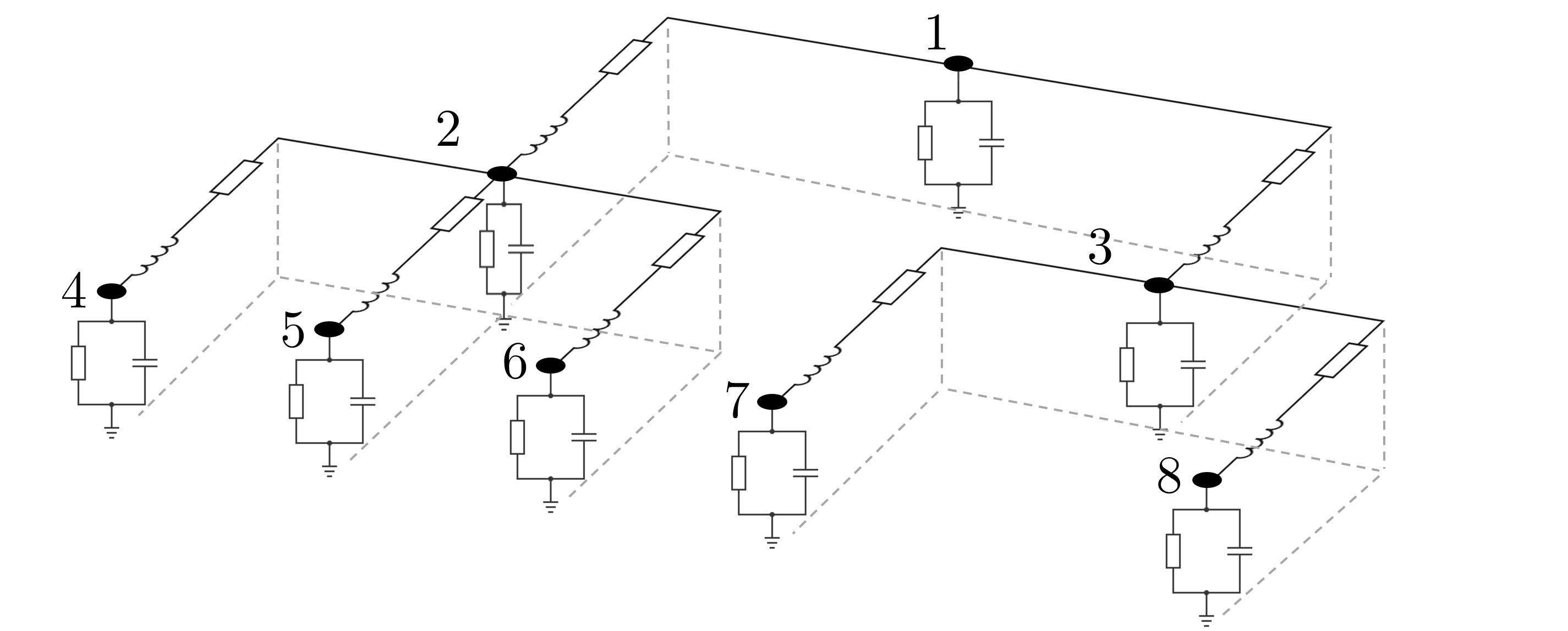
Figure 2: An 8-node DC power system.

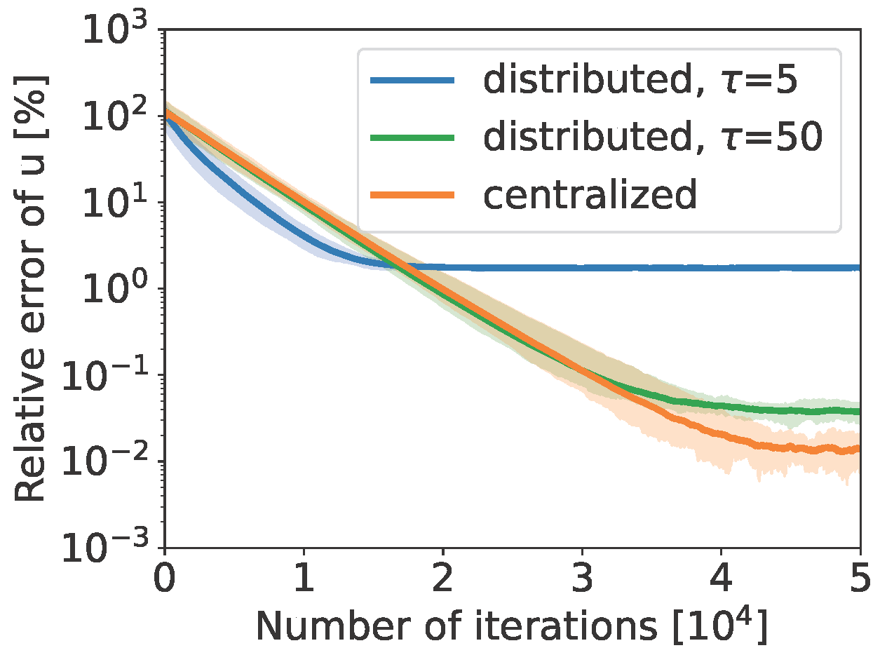
(a) Input error (unconstrained)

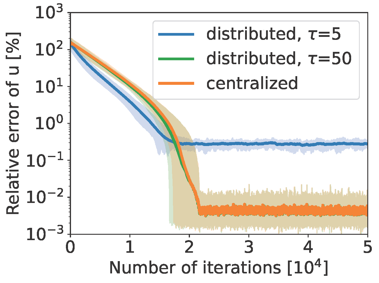
(b) Input error (constrained)

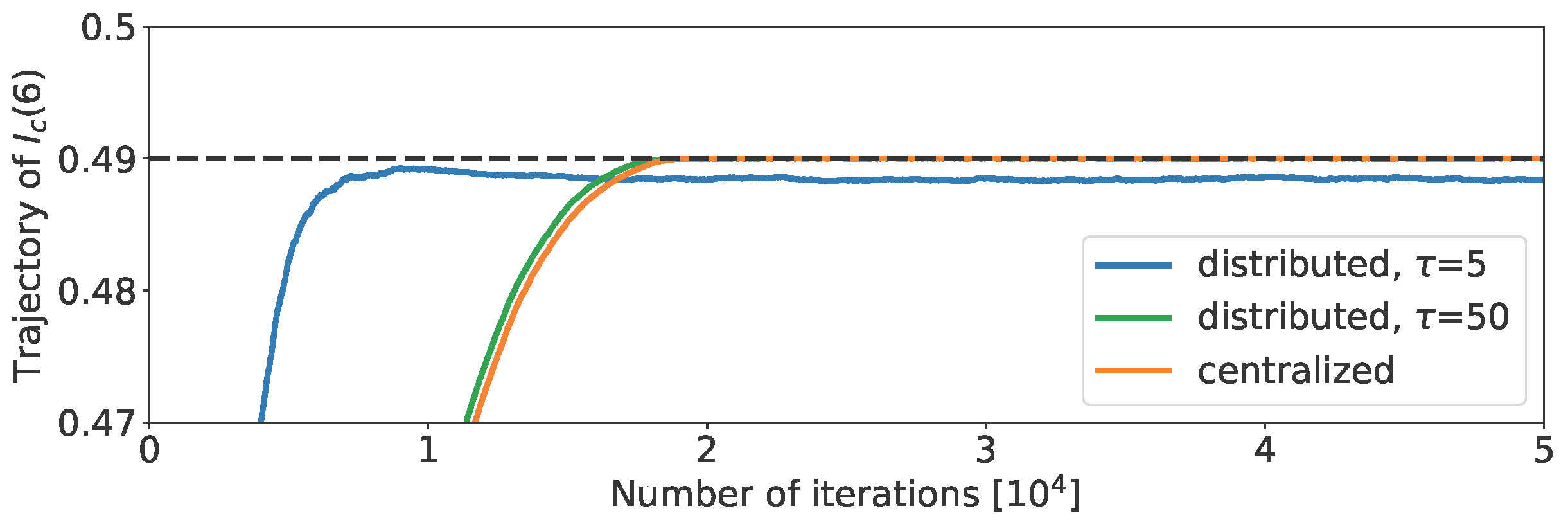
(c) Trajectory for constrained input $I_{c}(6)$ (averaged results)

Figure 3: Results for the distributed and centralized model-free controllers on a DC power system.

For the unconstrained problem, we plot the relative errors (i.e., $\|u_{k}-u^{*}\|/\|u^{*}\|$) in Fig. 3a. The solid line represents the average value over $20$ independent numerical experiments. The blue curve and green curve correspond to the distributed model-free OFO controller (7) with $\tau=5$ and $\tau=50$, respectively. The orange curve represents the centralized counterpart (i.e., when $\tau$ is set to zero and $W^{\tau}$ is replaced by $\frac{1}{N}\mathbf{1}\mathbf{1}^{\top}$ in (7)). They all own a linear convergence rate. The steady-state sub-optimality of the distributed controller (7) results from the error of zeroth-order gradient estimates and the finite consensus iterations reflected in $W^{\tau}$. As $\tau$ increases from $5$ to $50$, the performance of the distributed controller approaches that of the centralized controller.

In the scenario where input constraints are present, the convergence results are shown in Fig. 3b. Similar to the unconstrained scenario, the distributed controller enjoys a fast convergence rate. The gap between the distributed and centralized controllers decreases as we increase $\tau$. Constraint satisfaction is illustrated by the averaged trajectory of the input $I_{c}(6)$ in Fig. 3c, where the black dashed line represents the upper bound on the input. By exchanging more data (i.e., increasing $\tau$), the distributed controller converges to the optimal point, which is at the boundary of the feasible set.

VI Conclusion

In this paper, we proposed a distributed online feedback optimization controller to optimize the steady-state performance of a networked nonlinear system. This controller features fully model-free operations, moderate costs of local computations and communication, and closed-loop guarantees on optimality and constraint satisfaction. These benefits were achieved via a consensus-based protocol that exploits a queue of local objective values to track the global objective, as well as iterative local updates involving gradient estimates and projection. Future directions include asynchronous implementations to handle delays or packet drops and extensions to other applications, e.g., traffic networks and process control systems.

-A Proof of a Supporting Lemma

We first provide a useful lemma, which will be implemented in the following proofs. Let $\mathcal{F}_{k}$ be the $\sigma$-algebra (see [33, Section 1.2]) on the set formed by the random signals $v_{0},\ldots,v_{k-1}$. From [25, Lemma 5], we have

$$\mathbb{E}[\tilde{\nabla}\tilde{\Phi}(u_{k-\tau})|\mathcal{F}_{k-\tau}]=\nabla\tilde{\Phi}_{\delta}(u_{k-\tau}).$$

We further define

$$\mathbb{E}[\|\tilde{\nabla}\tilde{\Phi}(u_{0})\!+\!e_{0}\|^{2}]\!=\!\max_{p,q\in[\tau]}\{\mathbb{E}[\|\frac{1}{\delta}(W^{p}\varphi_{0}\!-\!W^{q}\varphi^{\text{init}}_{0})\odot v_{0}\|^{2}]\},$$

where $\varphi^{\text{init}}_{0}=[\tilde{\Phi}_{1}(u_{0}+\delta v^{\text{init}}_{0}),\ldots,\tilde{\Phi}_{N}(u_{0}+\delta v^{\text{init}}_{0})]^{\top}$, $v^{\text{init}}_{0}$ and $v_{0}$ both follow $\mathcal{N}(0,I_{N\times N})$.

Lemma 2.

Let $i,j\in\{1,\ldots,N\}$. If $1<k<\tau+2$,

$$\mathbb{E}[(\tilde{\Phi}_{j}( u_{k}+\delta v_{k})-\tilde{\Phi}_{j}(u_{k-1}+\delta v_{k-1}))^{2}v_{k}(i)^{2}]$$

$$\leq 2L_{0}^{2}\eta^{2}\mathbb{E}[\|\tilde{\nabla}\tilde{\Phi}(u_{0})+e_{0}\|^{2}]+8L_{0}^{2}\delta^{2}(N+1).$$

If $k\geq\tau+2$,

$$\mathbb{E}[(\tilde{\Phi}_{j}( u_{k}+\delta v_{k})-\tilde{\Phi}_{j}(u_{k-1}+\delta v_{k-1}))^{2}v_{k}(i)^{2}]$$

$$\leq 2L_{0}^{2}\eta^{2}\mathbb{E}[\|\tilde{\nabla}\tilde{\Phi}(u_{k-\tau-1})+e_{k-\tau-1}\|^{2}]+8L_{0}^{2}\delta^{2}(N+1).$$

Proof.

The upper bound is derived as follows

$$\mathbb{E}[( \tilde{\Phi}_{j}(u_{k}+\delta v_{k})-\tilde{\Phi}_{j}(u_{k-1}+\delta v_{k-1}))^{2}v_{k}(i)^{2}]$$

$$= \mathbb{E}[\mathbb{E}[(\tilde{\Phi}_{j}(u_{k}+\delta v_{k})-\tilde{\Phi}_{j}(u_{k-1}+\delta v_{k})$$

$$+\tilde{\Phi}_{j}(u_{k-1}+\delta v_{k})-\tilde{\Phi}_{j}(u_{k-1}+\delta v_{k-1}))^{2}v_{k}(i)^{2}|\mathcal{F}_{k}]]$$

$$\leq 2L_{0}^{2}\mathbb{E}[\mathbb{E}[\|u_{k}-u_{k-1}\|^{2}v_{k}(i)^{2}|\mathcal{F}_{k}]]$$

$$+2L_{0}^{2}\delta^{2}\mathbb{E}[\mathbb{E}[\|v_{k}-v_{k-1}\|^{2}v_{k}(i)^{2}|\mathcal{F}_{k}]]$$

$$\leq 2L_{0}^{2}\mathbb{E}[\mathbb{E}[\|u_{k}-u_{k-1}\|^{2}v_{k}(i)^{2}|\mathcal{F}_{k}]]+8L_{0}^{2}\delta^{2}(N+1).$$

If $1<k<\tau+2$,

$$\mathbb{E}[( \tilde{\Phi}_{j}(u_{k}+\delta v_{k})-\tilde{\Phi}_{j}(u_{k-1}+\delta v_{k-1}))^{2}v_{k}(i)^{2}]$$

$$\leq 2L_{0}^{2}\eta^{2}\mathbb{E}[\|\tilde{\nabla}\tilde{\Phi}(u_{0})+e_{0}\|^{2}]+8L_{0}^{2}\delta^{2}(N+1).$$

If $k\geq\tau+2$,

$$\mathbb{E}[( \tilde{\Phi}_{j}(u_{k}+\delta v_{k})-\tilde{\Phi}_{j}(u_{k-1}+\delta v_{k-1}))^{2}v_{k}(i)^{2}]$$

$$\leq 2L_{0}^{2}\eta^{2}\mathbb{E}[\|\tilde{\nabla}\tilde{\Phi}(u_{k\!-\!\tau\!-\!1})\!+\!e_{k\!-\!\tau\!-\!1}\|^{2}]\!+\!8L_{0}^{2}\delta^{2}(N\!+\!1).$$

-B Proof of Lemma 1

Proof.

We first provide an upper bound on $\mathbb{E}[\|e_{k}\|^{2}]$

$$\mathbb{E}[\| e_{k}\|^{2}]$$

$$= \frac{1}{\delta^{2}}\mathbb{E}\Big{[}\mathbb{E}\Big{[}\sum_{i=1}^{N}v_{k}(i)^{2}\Big{(}\sum_{j=1}^{N}(\Delta W)_{ij}(\varphi_{j,k}-\varphi_{j,k-1})\Big{)}^{2}|\mathcal{F}_{k}\Big{]}\Big{]}$$

$$\leq \frac{N}{\delta^{2}}\mathbb{E}\Big{[}\mathbb{E}\Big{[}\sum_{i=1}^{N}v_{k}(i)^{2}\Big{(}\sum_{j=1}^{N}(\Delta W)_{ij}^{2}(\varphi_{j,k}-\varphi_{j,k-1})^{2}\Big{)}|\mathcal{F}_{k}\Big{]}\Big{]},$$

where $\Delta W=W^{\tau}-\frac{1}{N}\mathbf{1}\mathbf{1}^{\top}$. From Lemma 2, if $1<k<\tau+2$,

$$\mathbb{E}[\|e_{k} \|^{2}]$$

$$\leq \frac{N}{\delta^{2}}\left(2L_{0}^{2}\eta^{2}\mathbb{E}[\|\tilde{\nabla}\tilde{\Phi}(u_{0})+e_{0}\|^{2}]+8L_{0}^{2}\delta^{2}(N+1)\right)$$

$$\cdot\sum_{i=1}^{N}\sum_{j=1}^{N}(W^{\tau}-\frac{1}{N}\mathbf{1}\mathbf{1}^{\top})_{ij}^{2}$$

$$\leq \frac{2N}{\delta^{2}}L_{0}^{2}\eta^{2}\text{tr}[(W^{\tau}-\frac{1}{N}\mathbf{1}\mathbf{1}^{\top})^{2}]\mathbb{E}[\|\tilde{\nabla}\tilde{\Phi}(u_{0})+e_{0}\|^{2}]$$

$$+ 8L_{0}^{2}\text{tr}[(W^{\tau}-\frac{1}{N}\mathbf{1}\mathbf{1}^{\top})^{2}](N+4)^{2}.$$

When $k\geq\tau+2$,

$$\mathbb{E}[\|e_{k} \|^{2}]$$

$$\leq \frac{2N}{\delta^{2}}L_{0}^{2}\eta^{2}\text{tr}[(W^{\tau}\!-\!\frac{1}{N}\mathbf{1}\mathbf{1}^{\top})^{2}]\mathbb{E}[\|\tilde{\nabla}\tilde{\Phi}(u_{k\!-\!\tau\!-\!1})\!+\!e_{k\!-\!\tau\!-\!1}\|^{2}]$$

$$+ 8L_{0}^{2}\text{tr}[(W^{\tau}-\frac{1}{N}\mathbf{1}\mathbf{1}^{\top})^{2}](N+4)^{2}.$$

For $\mathbb{E}[\|\tilde{\nabla}\tilde{\Phi}(u_{k})\|^{2}]$, by following a similar reasoning as the proof for Lemma 2, we have

$$\mathbb{E}[\|\tilde{\nabla}\tilde{\Phi}(u_{k})\|^{2}]\leq\frac{2N}{\delta^{2}}L_{0}^{2}\mathbb{E}[\mathbb{E}[\|u_{k}-u_{k-1}\|^{2}|\mathcal{F}_{k}]]+8L_{0}^{2}(N+4)^{2}.$$

If $1<k<\tau+2$,

$$\mathbb{E}[\|\tilde{\nabla}\tilde{\Phi}(u_{k})\|^{2}]\leq \frac{2N}{\delta^{2}}L_{0}^{2}\eta^{2}\mathbb{E}[\|\tilde{\nabla}\tilde{\Phi}(u_{0})+e_{0}\|^{2}]+8L_{0}^{2}(N+4)^{2}.$$

If $k\geq\tau+2$,

$$\mathbb{E}[\|\tilde{\nabla}\tilde{\Phi}(u_{k})\|^{2}]\leq \frac{2N}{\delta^{2}}L_{0}^{2}\eta^{2}\mathbb{E}[\|\tilde{\nabla}\tilde{\Phi}(u_{k-\tau-1})+e_{k-\tau-1}\|^{2}]$$

$$+8L_{0}^{2}(N+4)^{2}.$$

For $\mathbb{E}[\|\tilde{\nabla}\tilde{\Phi}(u_{k})+e_{k}\|^{2}]$, when $1<k<\tau+2$, we can establish an upper bound as follows

$$\mathbb{E}[\| \tilde{\nabla}\tilde{\Phi}(u_{k})+e_{k}\|^{2}]\leq 2\mathbb{E}[\|\tilde{\nabla}\tilde{\Phi}(u_{k})\|^{2}]+2\mathbb{E}[\|e_{k}\|^{2}]$$

$$\leq 2(\frac{2N}{\delta^{2}}L_{0}^{2}\eta^{2}\mathbb{E}[\|\tilde{\nabla}\tilde{\Phi}(u_{0})+e_{0}\|^{2}]+8L_{0}^{2}(N+4)^{2})$$

$$+2(\frac{2N}{\delta^{2}}L_{0}^{2}\eta^{2}\text{tr}[(W^{\tau}-\frac{1}{N}\mathbf{1}\mathbf{1}^{\top})^{2}]\mathbb{E}[\|\tilde{\nabla}\tilde{\Phi}(u_{0})+e_{0}\|^{2}]$$

$$+8L_{0}^{2}\text{tr}[(W^{\tau}-\frac{1}{N}\mathbf{1}\mathbf{1}^{\top})^{2}](N+4)^{2})$$

$$= \frac{4N}{\delta^{2}}L_{0}^{2}\eta^{2}\text{tr}[W^{2\tau}]\mathbb{E}[\|\tilde{\nabla}\tilde{\Phi}(u_{0})\!+\!e_{0}\|^{2}]\!+\!16L_{0}^{2}\text{tr}[W^{2\tau}](N\!+\!4)^{2}$$

$$\leq \frac{1}{\alpha}\mathbb{E}[\|\tilde{\nabla}\tilde{\Phi}(u_{0})+e_{0}\|^{2}]+16L_{0}^{2}\text{tr}[W^{2\tau}](N+4)^{2}\frac{1}{1-\alpha},$$

where $\alpha=\frac{4N}{\delta^{2}}L_{0}^{2}\eta^{2}\text{tr}[W^{2\tau}]$, and the parametric conditions ensure that $\alpha<1$.When $k\geq\tau+2$, we similarly have

$$\mathbb{E}[\|\tilde{\nabla} \tilde{\Phi}(u_{k})+e_{k}\|^{2}]$$

$$\leq \frac{4N}{\delta^{2}}L_{0}^{2}\eta^{2}\text{tr}[W^{2\tau}]\cdot\mathbb{E}[\|\tilde{\nabla}\tilde{\Phi}(u_{k-\tau-1})+e_{k-\tau-1}\|^{2}]$$

$$+16L_{0}^{2}\text{tr}[W^{2\tau}](N+4)^{2}$$

$$\overset{\text{(s.1)}}{\leq} \frac{1}{\alpha}\mathbb{E}[\|\tilde{\nabla}\tilde{\Phi}(u_{0})+e_{0}\|^{2}]+16L_{0}^{2}\text{tr}[W^{2\tau}](N+4)^{2}\frac{1}{1-\alpha}.$$

The right-hand side of (s.1) is $R$ in Lemma 1.

For $\mathbb{E}[\|\tilde{\nabla}\tilde{\Phi}(u_{k})\|^{2}]$, we have

$$\mathbb{E}[\|\tilde{\nabla}\tilde{\Phi}(u_{k})\|^{2}]\leq \frac{2N}{\delta^{2}}L_{0}^{2}\eta^{2}R+8L_{0}^{2}(N+4)^{2}$$

$$\overset{\text{(s.1)}}{=} \frac{\alpha R}{2\text{tr}[W^{2\tau}]}+8L_{0}^{2}(N+4)^{2}.$$

The right-hand side of (s.1) is $R_{f}$ in Lemma 1.

For $\mathbb{E}[\|e_{k}\|^{2}]$, we have

$$\mathbb{E}[\|e_{k}\|^{2}]\leq \frac{2N}{\delta^{2}}L_{0}^{2}\eta^{2}\text{tr}[(W^{\tau}-\frac{1}{N}\mathbf{1}\mathbf{1}^{\top})^{2}]R$$

$$+8L_{0}^{2}\text{tr}[(W^{\tau}-\frac{1}{N}\mathbf{1}\mathbf{1}^{\top})^{2}](N+4)^{2}$$

$$\overset{\text{(s.1)}}{=} \text{tr}[(W^{\tau}-\frac{1}{N}\mathbf{1}\mathbf{1}^{\top})^{2}]R_{f}.$$

The right-hand side of (s.1) is $R_{e}$ in Lemma 1. ∎

-C Proof for Theorem 1

Proof.

For $k\geq\tau+1$, we can bound $\mathbb{E}[\|u_{k+1}-u^{*}\|^{2}]$ via

$$\mathbb{E}[\| u_{k+1}-u^{*}\|^{2}]$$

$$= \mathbb{E}[\|u_{k}-u^{*}-\eta(\tilde{\nabla}\tilde{\Phi}(u_{k-\tau})+e_{k-\tau})\|^{2}]$$

$$= \mathbb{E}[\|u_{k}-u^{*}\|^{2}-2\eta(\tilde{\nabla}\tilde{\Phi}(u_{k-\tau})+e_{k-\tau})^{\top}(u_{k}-u^{*})$$

$$\quad+\eta^{2}\|\tilde{\nabla}\tilde{\Phi}(u_{k-\tau})+e_{k-\tau}\|^{2}]$$

$$\leq \mathbb{E}[\|u_{k}\!-\!u^{*}\|^{2}-2\eta\tilde{\nabla}\tilde{\Phi}(u_{k-\tau})^{\top}(u_{k}-u^{*})$$

$$\quad+\eta\|e_{k-\tau}\|^{2}+\eta\|u_{k}-u^{*}\|^{2}+\eta^{2}\|\tilde{\nabla}\tilde{\Phi}(u_{k-\tau})+e_{k-\tau}\|^{2}].$$

We use Lemma 1 to obtain

$$\mathbb{E}[ \|u_{k+1}-u^{*}\|^{2}]\leq\mathbb{E}[(1+\eta)\|u_{k}-u^{*}\|^{2}]$$

$$-\mathbb{E}[2\eta\tilde{\nabla}\tilde{\Phi}(u_{k-\tau})^{\top}(u_{k}-u^{*})]+\eta R_{e}+\eta^{2}R$$

$$= \mathbb{E}[(1+\eta)\|u_{k}-u^{*}\|^{2}]+\eta R_{e}+\eta^{2}R$$

$$-2\eta\underbrace{\mathbb{E}[\tilde{\nabla}\tilde{\Phi}(u_{k-\tau})^{\top}(u_{k-\tau}-u^{*})]}_{\text{(a)}}$$

$$-2\eta\underbrace{\mathbb{E}[\nabla\tilde{\Phi}(u_{k})^{\top}(u_{k}-u_{k-\tau})]}_{\text{(b)}}$$

$$-2\eta\underbrace{\mathbb{E}[(\tilde{\nabla}\tilde{\Phi}(u_{k})-\nabla\tilde{\Phi}(u_{k}))^{\top}(u_{k}-u_{k-\tau})]}_{\text{(c)}}$$

$$-2\eta\underbrace{\mathbb{E}[(\tilde{\nabla}\tilde{\Phi}(u_{k-\tau})-\tilde{\nabla}\tilde{\Phi}(u_{k}))^{\top}(u_{k}-u_{k-\tau})]}_{\text{(d)}}.$$

We establish upper bounds on terms (a)-(d). For (a), we have

$$-\mathbb{E}[\tilde{\nabla}\tilde{\Phi}(u_{k-\tau})^{\top} (u_{k-\tau}-u^{*})]\overset{\text{(s.1)}}{\leq}\mathbb{E}[\tilde{\Phi}_{\delta}(u^{*})-\tilde{\Phi}_{\delta}(u_{k-\tau})]$$

$$\overset{\text{(s.2)}}{\leq} \mathbb{E}[\tilde{\Phi}^{*}-\tilde{\Phi}(u_{k-\tau})]+\frac{L_{1}}{2}\delta^{2}N$$

$$\overset{\text{(s.3)}}{\leq} -\frac{m}{2}\mathbb{E}[\|u_{k-\tau}-u^{*}\|^{2}]+\frac{L_{1}}{2}\delta^{2}N,$$

where (s.1) follows from the convexity of $\tilde{\Phi}_{\delta}$; (s.2) uses the closeness between $\tilde{\Phi}_{\delta}$ and $\tilde{\Phi}$; (s.3) holds because $\tilde{\Phi}(u_{k-\tau})\geq\tilde{\Phi}^{*}+\frac{m}{2}\|u_{k-\tau}-u^{*}\|^{2}$. For (b), we have

$$-\nabla\tilde{\Phi}(u_{k})^{\top}(u_{k}\!-\!u_{k-\tau})\leq \tilde{\Phi}(u_{k-\tau})\!-\!\tilde{\Phi}(u_{k})\!-\!\frac{m}{2}\|u_{k-\tau}\!-\!u_{k}\|^{2}$$

$$\overset{\text{(s.1)}}{\leq} \tau L_{0}\sqrt{R}\eta-\frac{m}{2}\|u_{k-\tau}-u_{k}\|^{2},$$

where in (s.1) we rewrite $\tilde{\Phi}(u_{k})-\tilde{\Phi}(u_{k-\tau})$ as $\tilde{\Phi}(u_{k})-\tilde{\Phi}(u_{k-1})+\tilde{\Phi}(u_{k-1})-\cdots+\tilde{\Phi}(u_{k-\tau+1})-\tilde{\Phi}(u_{k-\tau})$ and use the convexity of $\tilde{\Phi}$. For (c), we have

$$\mathbb{E}[(\tilde{\nabla}\tilde{\Phi} (u_{k})-\nabla\tilde{\Phi}(u_{k}))^{\top}(u_{k}-u_{k-\tau})]$$

$$\leq \eta\mathbb{E}[\frac{1}{2}\|\nabla\tilde{\Phi}_{\delta}(u_{k})-\nabla\tilde{\Phi}(u_{k})\|^{2}$$

$$+\frac{1}{2}\|\tilde{\nabla}\tilde{\Phi}(u_{k-1})+e_{k-1}+\dots+\tilde{\nabla}\tilde{\Phi}(u_{k-\tau})+e_{k-\tau}\|^{2}]$$

$$\leq \frac{1}{2}\delta^{2}NL_{1}^{2}\eta+\frac{1}{2}\tau R\eta.$$

For (d), we have

$$\mathbb{E}[(\tilde{\nabla}\tilde{\Phi} (u_{k-\tau})-\tilde{\nabla}\tilde{\Phi}(u_{k}))^{\top}(u_{k}-u_{k-\tau})]$$

$$\leq \eta\mathbb{E}[\|\tilde{\nabla}\tilde{\Phi}(u_{k-\tau})-\tilde{\nabla}\tilde{\Phi}(u_{k})\|$$

$$\cdot\|\tilde{\nabla}\tilde{\Phi}(u_{k-1})+e_{k-1}+\dots+\tilde{\nabla}\tilde{\Phi}(u_{k-\tau})+e_{k-\tau}\|]$$

$$\leq \eta\mathbb{E}[\|\tilde{\nabla}\tilde{\Phi}(u_{k-\tau})\|^{2}+\|\tilde{\nabla}\tilde{\Phi}(u_{k})\|^{2}$$

$$+\frac{1}{2}\|\tilde{\nabla}\tilde{\Phi}(u_{k-1})+e_{k-1}+\dots+\tilde{\nabla}\tilde{\Phi}(u_{k-\tau})+e_{k-\tau}\|^{2}]$$

$$\leq 2\eta R_{f}+\frac{1}{2}\tau R\eta.$$

Hence, we can bound $\mathbb{E}[\|u_{k+1}-u^{*}\|^{2}]$ by

$$\mathbb{E}[\| u_{k+1}-u^{*}\|^{2}]\overset{\text{(s.1)}}{\leq}\mathbb{E}[(1+\eta)\|u_{k}-u^{*}\|^{2}]$$

$$-m\eta\mathbb{E}[(\|u_{k}-u^{*}\|^{2}+2(u_{k}-u_{k-\tau})^{\top}(u^{*}-u_{k-\tau}))]$$

$$\!+\!(2\tau L_{0}\sqrt{R}\!+\!\delta^{2}L_{1}^{2}N\!+\!2\tau R\!+\!4R_{f}\!+\!R)\eta^{2}\!+\!(R_{e}\!+\!L_{1}\delta^{2}N)\eta$$

$$\overset{\text{(s.2)}}{\leq} (1-(m-1)\eta+m\eta^{2})\mathbb{E}[\|u_{k}-u^{*}\|^{2}]+2m\tau R\eta^{3}$$

$$+(2\tau L_{0}\sqrt{R}+\delta^{2}L_{1}^{2}N+2\tau R+4R_{f}+m\tau R+R)\eta^{2}$$

$$+(R_{e}+L_{1}\delta^{2}N)\eta,$$ (14)

where in (s.1) we incorporate the above upper bounds on (a)-(d). In (s.2), we bound $-\mathbb{E}[(u_{k}-u_{k-\tau})^{\top}(u^{*}-u_{k-\tau})]$ by

$$-\mathbb{E}[( u_{k}-u_{k-\tau})^{\top}(u^{*}-u_{k-\tau})]$$

$$\leq \mathbb{E}[\|u_{k}\!-\!u_{k\!-\!1}\!+\!u_{k\!-\!1}-\dots\!+\!u_{k-\tau\!+\!1}\!-\!u_{k\!-\!\tau}\|\|u^{*}-u_{k-\tau}\|]$$

$$= \eta\mathbb{E}[\|\tilde{\nabla}\tilde{\Phi}(u_{k-1})+e_{k-1}+\dots+\tilde{\nabla}\tilde{\Phi}(u_{k-\tau})+e_{k-\tau}\|$$

$$\cdot\|u^{*}-u_{k}+u_{k}-u_{k-\tau}\|]$$

$$\leq \eta\mathbb{E}[(\frac{1}{2}+\eta)\|\tilde{\nabla}\tilde{\Phi}(u_{k-1})+e_{k-1}$$

$$+\dots+\tilde{\nabla}\tilde{\Phi}(u_{k-\tau})+e_{k-\tau}\|^{2}+\frac{1}{2}\|u^{*}-u_{k}\|^{2}]$$

$$= \frac{\eta}{2}\mathbb{E}[\|u^{*}-u_{k}\|^{2}]+(\frac{\eta}{2}+\eta^{2})\tau R.$$

We define $\rho=1-(m-1)\eta+m\eta^{2}$ and $p(\eta)=a_{1}\eta^{3}+a_{2}\eta^{2}+a_{3}\eta$, where

$$\begin{cases}a_{1}\!=\!2m\tau R,\\ a_{2}\!=\!2\tau L_{0}\sqrt{R}\!+\!\delta^{2}L_{1}^{2}N\!+\!2\tau R\!+\!4R_{f}\!+\!m\tau R\!+\!R,\\ a_{3}\!=\!R_{e}+L_{1}\delta^{2}N.\end{cases}$$ (15)

We telescope the inequality (-C) and arrive at (10). ∎

-D Proof for Corollary 1

Proof.

From Lemma 1, we have

$$\frac{p(\eta)}{1-\rho}=\frac{a_{1}\eta^{2}+a_{2}\eta+a_{3}}{(m-1)-m\eta}=\frac{a_{1}\eta^{2}+a_{2}\eta+R_{e}+L_{1}\delta^{2}N}{(m-1)-m\eta}.$$

By invoking the parametric conditions of $\eta_{\epsilon}$ and $\delta$, we obtain

$$\frac{p(\eta_{\epsilon})}{1-\rho}=\frac{\epsilon}{2}+\frac{R_{e}}{(m-1)-m\eta}.$$

If we select $\tau$ such that $\tau>\ln(\frac{(m-1-m\eta_{\epsilon})\epsilon}{2R_{f}(N-1)})/\ln(\lambda_{2}^{2})$, then

$$\frac{p(\eta_{\epsilon})}{1-\rho}<\frac{\epsilon}{2}+\frac{\epsilon}{2}<\epsilon.\qed$$

-E Proof for Theorem 2

Proof.

We derive the following recursive inequality of the expected distance to the optimal point

$$\mathbb{E}[\| u_{k+1}-u^{*}\|]=\mathbb{E}[\|\text{Proj}_{\mathcal{U}}[u_{k}-\eta(\tilde{\nabla}\tilde{\Phi}(u_{k-\tau})+e_{k-\tau})]$$

$$-\text{Proj}_{\mathcal{U}}[u^{*}-\eta(\tilde{\nabla}\tilde{\Phi}(u^{*})+e^{*})]\|]$$

$$\stackrel{{\scriptstyle\text{(s.1)}}}{{\leq}} \mathbb{E}[\|u_{k}\!-\!u^{*}\!-\!\eta\nabla\tilde{\Phi}(u_{k})\!-\!\eta\nabla\tilde{\Phi}(u^{*})\!+\!\eta(\nabla\tilde{\Phi}(u_{k})\!+\!\nabla\tilde{\Phi}(u^{*})$$

$$-(\tilde{\nabla}\tilde{\Phi}(u_{k-\tau})+e_{k-\tau})+(\tilde{\nabla}\tilde{\Phi}(u^{*})+e^{*}))\|]$$

$$\overset{\text{(s.2)}}{\leq} \sqrt{1-2m\eta+L_{1}^{2}\eta^{2}}\mathbb{E}[\|u_{k}\!-\!u^{*}\|]\!+\!\eta\mathbb{E}[\|\nabla\tilde{\Phi}(u_{k})\!+\!\nabla\tilde{\Phi}(u^{*})$$

$$-(\tilde{\nabla}\tilde{\Phi}(u_{k-\tau})+e_{k-\tau})+(\tilde{\nabla}\tilde{\Phi}(u^{*})+e^{*}\|]$$

$$\overset{\text{(s.3)}}{\leq} \sqrt{1-2m\eta+L_{1}^{2}\eta^{2}}\mathbb{E}[\|u_{k}-u^{*}\|]+2\eta L_{0}$$

$$+2\eta\sqrt{\frac{4ND_{\mathcal{U}}}{\delta^{2}}L_{0}^{2}\text{tr}[W^{2\tau}]+16L_{0}^{2}\text{tr}[W^{2\tau}](N+4)^{2}},$$

where (s.1) uses the non-expansiveness of the projection operator when the constraint set is convex; (s.2) follows by analyzing $\|u_{k}-u^{*}\|^{2}$ using the properties of strongly convex and smooth objectives; (s.3) is because a differentiable Lipschitz function has a bounded gradient. Moreover, the upper bound on $\mathbb{E}[\|\tilde{\nabla}\tilde{\Phi}(u_{k-\tau})+e_{k-\tau}\|]$ used in (s.3) is obtained by following similar reasoning as the proof for Lemma 1 and noting that the diameter of the feasible set is $D_{\mathcal{U}}$. We recursively apply the above inequality. Hence, (11) holds. ∎

References

• [1] A. Hauswirth, Z. He, S. Bolognani, G. Hug, and F. Dörfler, “Optimization algorithms as robust feedback controllers,” Annual Reviews in Control, vol. 57, p. 100941, 2024.
• [2] A. Simonetto, E. Dall’Anese, S. Paternain, G. Leus, and G. B. Giannakis, “Time-varying convex optimization: Time-structured algorithms and applications,” Proceedings of the IEEE, vol. 108, no. 11, pp. 2032–2048, 2020.
• [3] D. Krishnamoorthy and S. Skogestad, “Real-time optimization as a feedback control problem-A review,” Computers & Chemical Engineering, p. 107723, 2022.
• [4] J. W. Simpson-Porco, “Analysis and synthesis of low-gain integral controllers for nonlinear systems,” IEEE Transactions on Automatic Control, vol. 66, no. 9, pp. 4148–4159, 2021.
• [5] A. Hauswirth, F. Dörfler, and A. Teel, “Anti-windup approximations of oblique projected dynamics for feedback-based optimization,” arXiv preprint arXiv:2003.00478, 2020.
• [6] A. Hauswirth, S. Bolognani, G. Hug, and F. Dörfler, “Timescale separation in autonomous optimization,” IEEE Transactions on Automatic Control, vol. 66, no. 2, pp. 611–624, 2021.
• [7] V. Häberle, A. Hauswirth, L. Ortmann, S. Bolognani, and F. Dörfler, “Non-convex feedback optimization with input and output constraints,” IEEE Control Systems Letters, vol. 5, no. 1, pp. 343–348, 2021.
• [8] G. Belgioioso, D. Liao-McPherson, M. H. de Badyn, S. Bolognani, R. S. Smith, J. Lygeros, and F. Dörfler, “Online feedback equilibrium seeking,” arXiv preprint arXiv:2210.12088, 2022.
• [9] Z. He, S. Bolognani, J. He, F. Dörfler, and X. Guan, “Model-free nonlinear feedback optimization,” IEEE Transactions on Automatic Control, pp. 1–16, 2023.
• [10] G. Bianchin, J. Cortés, J. I. Poveda, and E. Dall’Anese, “Time-varying optimization of LTI systems via projected primal-dual gradient flows,” IEEE Transactions on Control of Network Systems, vol. 9, no. 1, pp. 474–486, 2021.
• [11] A. Bernstein, E. Dall’Anese, and A. Simonetto, “Online primal-dual methods with measurement feedback for time-varying convex optimization,” IEEE Transactions on Signal Processing, vol. 67, no. 8, pp. 1978–1991, 2019.
• [12] L. S. P. Lawrence, J. W. Simpson-Porco, and E. Mallada, “Linear-convex optimal steady-state control,” IEEE Transactions on Automatic Control, vol. 66, no. 11, pp. 5377–5384, 2021.
• [13] M. Colombino, E. Dall’Anese, and A. Bernstein, “Online optimization as a feedback controller: Stability and tracking,” IEEE Transactions on Control of Network Systems, vol. 7, pp. 422–432, 2020.
• [14] L. Ortmann, C. Rubin, A. Scozzafava, J. Lehmann, S. Bolognani, and F. Dörfler, “Deployment of an online feedback optimization controller for reactive power flow optimization in a distribution grid,” in IEEE PES ISGT Europe, 2023.
• [15] A. Nedic, A. Olshevsky, and M. G. Rabbat, “Network topology and communication computation tradeoffs in decentralized optimization,” Proceedings of the IEEE, vol. 106, no. 5, pp. 953–976, 2018.
• [16] W. Wang, Z. He, G. Belgioioso, S. Bolognani, and F. Dörfler, “Decentralized feedback optimization via sensitivity decoupling: Stability and sub-optimality,” in 2024 European Control Conference, accepted.
• [17] G. Belgioioso, S. Bolognani, G. Pejrani, and F. Dörfler, “Tutorial on congestion control in multi-area transmission grids via online feedback equilibrium seeking,” in 62nd IEEE Conference on Decision and Control, 2023, pp. 3995–4002.
• [18] C.-Y. Chang, M. Colombino, J. Corté, and E. Dall’Anese, “Saddle-flow dynamics for distributed feedback-based optimization,” IEEE Control Systems Letters, vol. 3, no. 4, pp. 948–953, 2019.
• [19] A. Bernstein and E. Dall’Anese, “Real-time feedback-based optimization of distribution grids: A unified approach,” IEEE Transactions on Control of Network Systems, vol. 6, no. 3, pp. 1197–1209, 2019.
• [20] X. Zhang, A. Papachristodoulou, and N. Li, “Distributed control for reaching optimal steady state in network systems: An optimization approach,” IEEE Transactions on Automatic Control, vol. 63, no. 3, pp. 864–871, 2018.
• [21] J. I. Poveda and A. R. Teel, “A robust event-triggered approach for fast sampled-data extremization and learning,” IEEE Transactions on Automatic Control, vol. 62, no. 10, pp. 4949–4964, 2017.
• [22] Y. Chen, A. Bernstein, A. Devraj, and S. Meyn, “Model-free primal-dual methods for network optimization with application to real-time optimal power flow,” in American Control Conference, 2020, pp. 3140–3147.
• [23] X. Chen, J. I. Poveda, and N. Li, “Safe model-free optimal voltage control via continuous-time zeroth-order methods,” in 60th IEEE Conference on Decision and Control, 2021, pp. 4064–4070.
• [24] Y. Nesterov and V. Spokoiny, “Random gradient-free minimization of convex functions,” Foundations of Computational Mathematics, vol. 17, pp. 527–566, 2017.
• [25] Y. Zhang, Y. Zhou, K. Ji, and M. M. Zavlanos, “A new one-point residual-feedback oracle for black-box learning and control,” Automatica, vol. 136, p. 110006, 2022.
• [26] X. Chen, Y. Tang, and N. Li, “Improve single-point zeroth-order optimization using high-pass and low-pass filters,” in International Conference on Machine Learning, 2022, pp. 3603–3620.
• [27] Y. Tang, Z. Ren, and N. Li, “Zeroth-order feedback optimization for cooperative multi-agent systems,” Automatica, vol. 148, p. 110741, 2023.
• [28] A. Maritan and L. Schenato, “ZO-JADE: Zeroth-order curvature-aware distributed multi-agent convex optimization,” IEEE Control Systems Letters, vol. 7, pp. 1813–1818, 2023.
• [29] O. Shamir, “An optimal algorithm for bandit and zero-order convex optimization with two-point feedback,” The Journal of Machine Learning Research, vol. 18, no. 1, pp. 1703–1713, 2017.
• [30] Y. Tang, J. Zhang, and N. Li, “Distributed zero-order algorithms for nonconvex multiagent optimization,” IEEE Transactions on Control of Network Systems, vol. 8, no. 1, pp. 269–281, 2020.
• [31] R. Dixit, A. S. Bedi, R. Tripathi, and K. Rajawat, “Online learning with inexact proximal online gradient descent algorithms,” IEEE Transactions on Signal Processing, vol. 67, no. 5, pp. 1338–1352, 2019.
• [32] J. Zhao and F. Dörfler, “Distributed control and optimization in DC microgrids,” Automatica, vol. 61, pp. 18–26, 2015.
• [33] R. B. Ash and C. A. Doleans-Dade, Probability and measure theory.   Academic press, 2000.