Dynamical typicality in elementary cellular automata

Abstract

We study the dynamics of elementary cellular automata (CA) using numerical simulations. We follow the dynamics of macroscopic observables, which depend on the state of a large number of sites. If we consider the ensemble of states that share the same value of some macroscopic observable, for example, the density, we find that the dynamics of such macroscopic observable is approximately the same for the vast majority of the states in the ensemble, irrespective of the microscopic details, provided that the system size $N$ is large enough. Moreover, we find that the dynamics of any other macroscopic observable is also very similar for members of the same ensemble. We show that the ensemble fluctuations around the average macro-trajectory vanish as $N^{-1/2}$, irrespective of the observable and the dynamical rule. We show that the same phenomenon is present if we define our initial condition ensemble by fixing more than one macroscopic observable. The ensuing “dynamical typicality” phenomenon is very similar to what was recently found in the context of the dynamics of isolated quantum systems. Our results suggest that the same feature is likely to be found in a wide variety of complex dynamical systems. We also discuss the implications of our findings regarding the ability of CA to simulate physical systems.

1 Introduction

We speak of typicality whenever a certain set of states of a system, grouped according to some common feature (drawn with the same probability distribution, sharing the same value of some relevant observable, etc.), yields a very sharp distribution of some other feature. Typicality is at the root of the predictive power of equilibrium statistical mechanics. In fact, as E. T. Jaynes argues in his landmark paper [1], the sole fact that matter has well defined macroscopic properties indicate that the vast majority of the accessible microstates share the same value of such macroscopic observables. Take for example the canonical distribution, which can be obtained as a maximum entropy estimate and is thus the broadest possible distribution compatible with the macroscopic information about the energy of the system. This distribution yields to enormously sharp peaks for any given macroscopic observable in all cases in which statistical mechanics makes predictions in agreement with experiments. This fact indicates that the vast majority of microstates with appreciable statistical weight share the same macroscopic behavior.

Several instances of typicality have been proven for quantum mechanical systems. First, it was discovered that for the overwhelming majority of the wave functions of a sufficiently large system that belong to a microcanonical window of energies, the reduced density matrix of any subsystem is well approximated by a canonical density matrix, a feature designated as “canonical typicality” [2, 3]. In Ref. 4 it is demonstrated that states drawn according to a certain probability distribution in Hilbert space feature very similar quantum expectation values of generic observables. Closer to our interest in the present paper, typicality arguments have been extended to encompass the dynamics of quantum systems. In a pioneering investigation, Bartsch and Gemmer demonstrated that the overwhelming majority of pure states in a set featuring a common expectation value of some observable $A$ at some time $t$, yield very similar expectation values at any later time [5]. Finally, in Ref. 6 it was shown that the vast majority of pure states with energies inside a microcanonical interval which at time $t=0$ have very similar values of some set of observables $A_{1},\ldots,A_{K}$ will exhibit very similar expectation values for any other observable $O$ at any later time. The reproducibility of macroscopic experiments in quantum systems rests upon this remarkable feature [6].

However, reproducible phenomena are ubiquitous, and so we would expect typicality to be present in systems outside the realm of quantum mechanics. As Jaynes puts it in Ref. 7:

If any macrophenomenon is found to be reproducible, then it follows that all microscopic details that were not reproduced, must be irrelevant for understanding and predicting it.

In other words, for deterministic systems, microscopic details in the preparation of the initial condition are irrelevant as long as the initial value of the relevant macroscopic observables can be reproduced.

It is thus natural to search for dynamical typicality in other types of dynamical systems. In the present paper we study the dynamics of large cellular automata (CA), which are among the most simple many body dynamical systems conceivable. CA are dynamical systems in which space, time and the states are discretized, and the dynamical evolution is implemented through uniform local rules that update the state of the system at each time step. Besides their simplicity, CA are attractive for our inquiry because they are used to model a wide variety of complex systems, like fluids, neural networks, ecologic and economic systems, chemical reaction-diffusion systems, crystal growth, pattern formation in living systems, traffic flow, urban segregation, etc. [9, 8]. Moreover, they can be regarded, in abstract, as models of complexity itself, and constitute a playground to study emergent properties in complex systems in its most essential form [9, 10]. In this work we focus on the most simple CA, one-dimensional chains of sites with two states evolving with a nearest neighbor rule, called elementary CA.

Through a series of numerical experiments, we lend support to the dynamical typicality picture in elementary CA, in which, for large systems, the vast majority of all initial states that share the same value of a given set of macroscopic observables, also generate, when evolved dynamically according to the given rule, very similar trajectories not only for the macroscopic observables that defines the ensemble, but also for any other macroscopic observable. In the course of our discussion we will provide a precise meaning to the expressions “vast majority” and “macroscopic observable”.

Just as “state typicality” is a powerful principle intimately related to the predictive power of equilibrium statistical mechanics, dynamic typicality is a good candidate to emerge as an organizing principle in non-equilibrium statistical mechanics [7].

The rest of the paper is organized as follows. In Section II we define the elementary CA and the observables that we will use to characterize the dynamics. In Section III we will present the results of our numerical investigations. Finally, in Section IV we will discuss some implications of our results, future perspectives and state our conclusions.

2 Model and observables

Among CA, the most simple ones are elementary CA. These are one dimensional chains of sites with two states, $0$ or $1$ or, using a color code, white and black (we will use both representations indistinctly throughout the paper). The rule to determine the state of the site in the next time step depends on the current state of the site and its two immediate neighbors. There are only $256$ different dynamical rules allowed under this scheme, which can be labeled using Wolfram’s numbering system, which assigns an integer between $0$ and $255$ to each rule. These rules can be classified into four classes according to the behavior of the system starting from a random state [8]. Class $1$ and $2$ show very simple dynamics either quickly reaching a uniform state (class $1$) or showing a repetitive pattern (class $2$). On the other hand, class $3$ shows apparently random or noisy dynamical patterns, while class $4$ rules produce a more complex and structured dynamics. We will focus on class $3$ and $4$ rules.

One important piece of information for our discussion is that the Hamming distance between nearby configurations, i.e. the number of sites at which the corresponding bits are different while comparing two configurations, diverges linearly for non-additive rules [11], like those used in the present paper. This means that in the course of the dynamical evolution nearby configurations become more and more different, a fact that indicates that any form of dynamical typicality is a non-trivial feature.

We consider elementary cellular automata with $N$ sites and periodic boundary conditions. We chose to work with Rule $110$, a member of class $4$, and Rule $126$ from class $3$. These rules will drive the evolution of the microstate of the system. At each time-step, the microstate of the system is described by an $N$-dimensional vector with components

$$s_{n}(m)=0,1,$$ (1)

where $n=1,\ldots,N$ is the spatial index and $m=1,\ldots,M$ labels the time step. In order to characterize the macroscopic state of the system we chose a set of macroscopic observables:

• The density of black sites,

  $$\rho(m)=\frac{1}{N}\sum^{N}_{n=1}\,s_{n}(m).$$ (2)

• The density on the left half of the system,

  $$\rho_{L}(m)=\frac{1}{N}\sum^{N/2}_{n=1}\,s_{n}(m).$$ (3)

• The density of “domain walls”, understood as the number of occurrences of the strings $01$ or $10$ in the microstate of the system; this density can be written as,

  $$\rho_{|}(m)=\frac{1}{N}\sum^{N-1}_{n=1}\,(1-\delta_{s_{n}(m),s_{n+1}(m)}).$$ (4)

• A suitable correlation function which can be calculated for each configuration,

  $$C_{2}(r,m)=\langle S_{n}(m)\,S_{n+r}(m)\rangle-\langle S_{n}(m)\rangle\langle S_{n+r}(m)\rangle,$$ (5)

  where $r=0,\ldots,N$, $\langle\ldots\rangle$ denotes the average over all the sites in the cellular automaton and $S_{n}$ takes the value $-1$ and $1$ when $s_{n}$ is equal to $0$ and $1$, respectively [11].

We can define a macrostate as the set of all different microstates which are compatible with given values of these macroscopic observables.

3 Initial states ensembles and dynamical typicality

For an $N$-site CA there are $2^{N}$ different states, which can be used as initial conditions for the dynamics. Since the system is deterministic, each initial condition generates one micro-trajectory, specified by $s_{n}(m)$, and each micro-trajectory is associated with a macro-trajectory, given by the set of time-dependent macroscopic observables. The main statement is that for very large $N$, the vast majority of the microstates belonging to the same macrostate have very similar macro-dynamics. To provide evidence supporting this claim, we will work mainly with the macrostate of fixed density. In order to get a qualitative picture of what happens as $N$ increases, in Fig. 1, panels (a) to (c), we show the dynamics of the density $\rho(m)$ for different initial conditions which share $\rho(1)=0.5$ evolved according to rule $110$. The initial conditions are constructed as random permutation of the half-filled state $1,1,\cdots,1,1,0,0,\cdots,0,0$ and are thus expected to be typical microstates. We can appreciate that the macrotrajectories of the density tend to collapse on the same curve as $N$ increases. Moreover, the same happens for all the other macroscopic observables under scrutiny (see panels (d) to (f)), even though we do not fix their initial values. In other words, as $N$ increases, for initial states belonging to the $\rho=0.5$ macrostate, the dynamics of the density and all other macroscopic observables becomes independent of the details of the initial conditions.

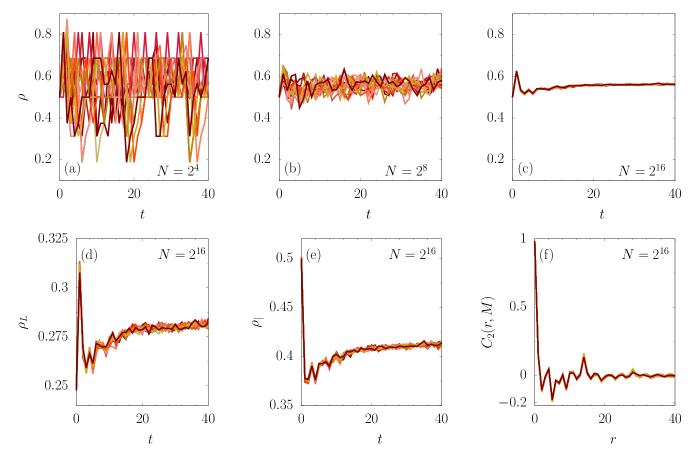
Figure 1: Dynamics of macroscopic observables for initial conditions with $\rho=0.5$, Rule $110$ (a)-(c) Sample trajectories of the density $\rho(m)$ for initial conditions with $\rho=0.5$ for different system sizes $N$. (d)-(f) Sample trajectories of other macroscopic observables for $N=2^{16}$ and the same initial conditions used in (c). In (f) $M=100$.

In order to get quantitative information we will consider the ensemble of all initial conditions with fixed $\rho=0.5$ density for a given value of $N$. We have checked that the results do not change qualitatively if we chose a different value for $\rho$. We will denote with $K$ the number of states that belong to such ensemble. We will systematically analyze the standard deviation of the macrotrajectories around the ensemble average as $N$ increases. We will define time averaged relative standard deviations for each macro-observable. For the density,

$$\overline{RSD}(\rho)=\frac{1}{M}\,\sum_{m=1}^{M}\,\frac{\sigma_{m}(\rho)}{\mu_{m}(\rho)},$$ (6)

where,

$$\mu_{m}(\rho)=\frac{1}{K}\,\sum_{k=1}^{K}\,\rho^{(k)}(m),$$ (7)

where $\rho^{(k)}(m)$ denotes the macro-trajectory for the $k$-th trajectory inside the fixed density ensemble, and,

$$\sigma_{m}(\rho)=\frac{1}{K^{1/2}}\,\sqrt{\sum_{k=1}^{K}\,\left(\mu_{m}(\rho)-\rho^{(k)}(m)\right)^{2}}.$$ (8)

We use analogous definitions for $\rho_{L}$ and $\rho_{|}$. To address the correlation function, we will study the time averaged absolute standard deviation of the correlation function evaluated at $r=N/2$

$$\overline{SD}(C_{2})=\frac{1}{M}\,\sum_{m=1}^{M}\,\sigma_{m}(C_{2}(N/2)),$$ (9)

because $C_{2}(N/2,m)$ is very close to zero.

For small systems we can use a brute force approach and calculate $\overline{RSD}(\rho)$, $\overline{RSD}(\rho_{L})$, $\overline{RSD}(\rho_{|})$ and $\overline{SD}(C_{2})$ using the ensemble encompassing all microstates with $\rho=0.5$. However, $K$ increases exponentially with $N$, which imposes a strong computational limit to this approach. For example, $K\sim\,10^{7}$ for $N=28$. In order to explores larger values of $N$ we must devise an approximate approach. We propose to replace the exact ensemble at fixed density with an ensemble of $K^{\prime}$ random states with fixed $\rho=0.5$. As we mentioned before, we can construct such states as random permutation of the half-filled state. In Fig. 2 we show the behavior of the averaged standard deviations as a function of $N$ for two different dynamical rules, both for the exact ensemble (up to $N=28$) and the random sampling approximation. We find that using $K^{\prime}=10^{4}$ leads to a very good convergence of the approximate and the exact results for the values of $N$ for which the exact approach is feasible. Note that, for example, for $N=10$, $K=252$, however we need a larger $K^{\prime}=10^{4}$ to obtain a good convergence. Nevertheless, $K$ grows very fast with $N$, and already for $N=28$, $K\gg K^{\prime}$. The approximation allow us to access very large system sizes. We can clearly observe that, independently of the observable and the dynamical rule, the fluctuations around the average macrotrajectory for the $\rho=0.5$ ensemble vanish as $N^{-1/2}$. When we say that the “vast majority of states” follow the same macrodynamics we thus mean that, for an ensemble in which all states have the same statistical weight, the relative fluctuations around the average macrotrajectory vanish with the system size.

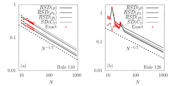
Figure 2: Decay of fluctuations with system size for Rule $110$ and $126$ (a) Decay of fluctuations for Rule $110$. Red (gray) dots are the exact results obtained using brute force approach in small systems. Lines are the results obtained with the random sampling approximation. We observe excellent agreement between both approaches where exact results are available. (b) Same as (a) but for Rule $126$. For this rule we see larger fluctuations for small system sizes. For all the points in this figure we used $M=30$.

With this piece of information at hand, we can ask for what kind of observables the above picture is valid. In order to answer this question we study the relative fluctuations of a certain group of observables, for the dynamics starting from states with fixed $\rho=0.5$ and at large but fixed $N=1000$ using the random sampling approximation. The observables that we chose to study are the block densities centered around the middle of the chain:

$$\rho_{b}(m)=\sum_{n=N/2-N_{b}/2}^{N/2+N_{b}/2}\,s_{n}(m),$$ (10)

where $N_{b}$ is the size of the block. In Fig. 3 we show the relative fluctuations of the trajectory of $\rho_{b}(m)$ around the average for different values of $N_{b}$. A little bit unsurprisingly, they decay as $N_{b}^{-1/2}$. We thus see that fluctuations disappear when we consider observables taking contributions from more and more sites of the chain. However, there is not a scale for which observables can be considered “macroscopic”.

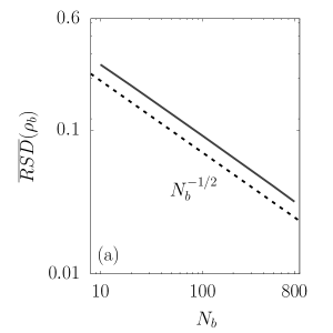
Figure 3: Decay of relative fluctuations of the block density $\rho_{b}(m)$ as a function of the size of the block $N_{b}$. Points were obtained using the random sampling approximation for a system with $N=1000$. We used $M=30$.

Finally, we want to check if typicality is valid if we consider initial conditions ensembles which fix more than one macroscopic observable. To this end we focus on the ensemble of initial conditions with $\rho=0.5$ and $\rho_{L}=0.1$. This represents a case in which there is a density imbalance between both halves of the system, similar to the Riemann problem. In Fig. 4 we show the macrotrajectories of the macroscopic observables for representatives of such ensemble for $N=2^{16}$. We can clearly see that all trajectories tend to collapse on the same curve, not only for $\rho$ and $\rho_{L}$, but for the other observables as well. We also show trajectories for the case in which we only fix $\rho=0.5$ in grey to show that, in general, the macrodynamics of both ensembles are different.

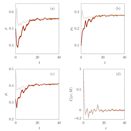
Figure 4: Macroscopic dynamics of initial conditions with $\rho=0.5$ and $\rho_{L}=0.1$ in a system with $N=2^{16}$. In (d) $M=100$.

Although we have investigated only a handful of observables, we conjecture that the same general picture described up to here will hold for any set of observables which depends on the state of a large number of sites, without giving too much weight to any one of them.

4 Conclusions and perspectives

We have provided numerical evidence for the existence of dynamical typicality in the macroscopic dynamics of elementary CA. The picture that have emerged can be described as follows:

Given a set of macroscopic observables, we can classify all possible ($2^{N}$) initial states according to the values that such set of observables take, irrespective of the microscopic details. Inside each class, the dynamics of all macro-observables (not only those used to define the classification) will be very similar, except for a group of atypical states whose statistical weight vanishes as $N$ increases.

We have clarified that by “macroscopic” we refer to an observable that depends on the state of a large number of cells, but not too much on any of them in particular. Moreover, we have shown that the vanishing of fluctuations goes like $N^{-1/2}$ irrespective of the observable and the details of the dynamical rule.

We conjecture that the same picture is valid for higher dimensional CA, and for more sophisticated dynamical rules.

For large $N$ the dynamics of the macroscopic observables is thus approximately determined by its own initial conditions and the dynamical rule applied. In this respect, we want to mention a connection between our results and a proposal made by Toffoli in Ref. 12. He proposed to use CA macro-observables to simulate physical quantities which are specified by continuous real-valued fields, such as charge and temperature. His specific proposal was to identify the density inside a sphere centered at each lattice with the value of the field whose dynamics is being simulated. He speculated that the dynamics of the field will be deterministic, i.e. determined solely by its initial conditions and the underlying dynamical rule, if the rule is suitable chosen and the radius of the sphere is in a suitable range. Our results suggest that the dynamics of the density field, and any other macroscopic observable, will be approximately deterministic if the size of the system is sufficiently large and the radius of the sphere is large also, irrespective of the underlying dynamical rule.

Regarding the results obtained for quantum systems, we should mention that in the quantum case even microscopic observables, like the quantum expectation value of a single spin in a spin chain, show typical dynamics for large system sizes [5]. This is at variance with what we found, since in elementary CA microscopic observables can show large fluctuations even for large systems.

As open problems and perspectives, it would be interesting to make progress trying to prove dynamical typicality in CA using analytical tools. One possible direction is to explore the relation between dynamical typicality in CA and the phenomenon of concentration of measure [13]. Both phenomena are indeed related in the quantum mechanical case [3]. Finally, it would be interesting to test the robustness of the dynamical typicality picture with respect to stochastic perturbations of the dynamics.

References

- [1] E.T. Jaynes, Information theory and Statistical mechanics, Phys. Rev. 106, 620 (1957).
- [2] S. Goldstein, J.L. Lebowitz, R. Tumulka, and N. Zanghì, Canonical typicality, Phys. Rev. Lett. 96, 050403 (2006).
- [3] S. Popescu, A.J. Short, and A. Winter, Entanglement and the foundations of statistical mechanics, Nature Physics 2, 754 (2006).
- [4] P. Reimann, Typicality for generalized microcanonical ensembles, Phys. Rev. Lett. 99, 160404 (2007).
- [5] C. Bartsch, and J. Gemmer, Dynamical typicality of quantum expectation values Phys Rev. Lett. 102, 110403 (2009).
- [6] P. Reimann and J. Gemmer, Why are macroscopic experiments reproducible? Imitating the behavior of an ensemble by single pure states Physica A: Statistical Mechanics and its applications 552, 121840 (2020).
- [7] E.T. Jaynes, Macroscopic prediction, In: H. Haken (eds) Complex Systems – Operational Approaches in Neurobiology, Physics and Computers. Springer Series in Synergetics, vol. 31. Springer, Berlin.
- [8] S. Wolfram, A new kind of science, Wolfram Media, 2002.
- [9] A. Ilachinski, Cellular automata: a discrete universe, World Scientific, 2001.
- [10] F. Berto, and J. Tagliabue, Cellular automata, The Stanford Encyclopedia of Philosophy (Winter 2023 edition).
- [11] S. Wolfram, Statistical mechanics of cellular automata, Rev. Mod. Phys. 5, 601 (1983).
- [12] T. Toffoli, Cellular automata as an alternative to (rather than an approximation of) differential equations in modeling physics, Physica D: Nonlinear phenomena 10, 117 (1984).
- [13] M. Talagrand, A new look at independence, The Annals of Probability 24, 1 (1996).