Evaluating Explanatory Capabilities of Machine Learning Models in Medical Diagnostics: A Human-in-the-Loop Approach

Abstract

This paper presents a comprehensive study on the evaluation of explanatory capabilities of machine learning models, with a focus on Decision Trees, Random Forest and XGBoost models using a pancreatic cancer dataset. We use Human-in-the-Loop related techniques and medical guidelines as a source of domain knowledge to establish the importance of the different features that are relevant to establish a pancreatic cancer treatment. These features are not only used as a dimensionality reduction approach for the machine learning models, but also as way to evaluate the explainability capabilities of the different models using agnostic and non-agnostic explainability techniques. To facilitate interpretation of explanatory results, we propose the use of similarity measures such as the Weighted Jaccard Similarity coefficient. The goal is to not only select the best performing model but also the one that can best explain its conclusions and aligns with human domain knowledge.

1 Introduction

Explainable AI (XAI) [1] is a research field focused on making Artificial Intelligence (AI) systems in general, and Machine Learning (ML) systems in particular, more understandable to humans. Explainable AI offers several advantages, to name a few: it fosters confidence in the prediction of the model by making the decision-making process more transparent, promotes responsible AI development, aids in debugging and identifying issues, and allows auditing of AI models and checking if they adhere to regulatory standards.

The inherent explainability of AI systems has not remained static but has changed considerably as a result of technological progress. In fact, explainability has become an increasingly difficult issue to tackle, as the internal functioning of AI systems has become less intelligible as they have become more complex [2].

Initially, symbolic AI models were explainable per se, e.g., rule-based expert systems could easily show to their users which rules they had followed to make a given decision, even though the rules can incorporate measures of uncertainty and imprecision as, for example, in fuzzy systems. These type of AI models are considered transparent, which means that the model itself is understandable [3], being understandability the characteristic of a model to make a human understand its function without any need for explaining its internal structure or the algorithmic means by which the model processes data internally [4].

However, rule-based systems presented too many limitations that hindered their development: they were rigid systems, with poor scalability and limited learning capabilities. To overcome the problems associated with symbolic AI, machine learning models were developed. These models can learn from data and improve their performance over time without being explicitly programmed. They are obviously very dependent on data to obtain their results, but, in general, their performance, scalability, and generalization features are superior to those present on symbolic models.

But these machine learning models often lack interpretability. Some of them can be considered transparent, such as Logistic Regression or Decision Trees, but these are usually the simplest models that offer lower performance in complex domains. More complex models such as Random Forest, Support Vector Machines, Neural Networks, and models based on Deep Learning (convolutional networks, recurrent networks, etc.) are opaque models. We can see that there seems to be a trade-off between model interpretability and model performance. More interpretable models tend to perform less well than less interpretable models.

Therefore, the main question is not whether it is possible to arrive at explainable solutions—this has been true for a long time—but whether it is possible to obtain explainable solutions with an accuracy that is comparable to the highly effective but comparably opaque Deep Learning systems [2].

In an attempt to include explainability into the opaque models, “agnostic” techniques have been developed, which can be applied seamlessly to any ML model, regardless of its inner processing or internal representations [3]. The problem with these agnostic or post-hoc explainability methods is their reliability. Some authors [5] pointed out that they are inconsistent, unstable, and provide very little insight into their correctness and reliability, in addition to being computationally inefficient. It is therefore necessary to develop some way of validating the explanatory capabilities obtained by these models, especially in complex domains, such as medical environments, where it may not be easy to determine the correct answer to a given problem.

In this article, we face a problem related to pancreatic cancer, deciding the best treatment for a patient given his or her clinical characteristics. Since our dataset is tabular in nature and does not have too many cases, we decided to try to solve the problem using classical machine learning models, such as Decision Trees (DT) [6], Random Forest (RF) [7], or XGBoost models [8]. We have already seen that DT are transparent models, but RF and XGBoost are opaque.

Since we are in a medical domain, we understand that the models must offer adequate explainability, but how can we validate the results? A first way would be to apply different methods of explainability on the same model and compare the results with each other. But we want to go further and check if the explainability of the models has medical significance, which would allow us to have more trust in them.

To verify the medical significance, we can rely on the opinions of medical experts and also use medical guidelines that act as a “gold standard” in the field. The former option involves some kind of Human-in-the-Loop (HITL) approach [9], which is often a complex process and require the active participation of human experts. The latter option relies on bibliography and manuals, which tend to be exhaustive and sometimes hard to navigate through.

The contribution of this paper is, in addition to the comparison between models of explainability, the development of different ways of evaluation of explainability models based on the collaboration of human experts and the guidelines available in the domain and its application to a pancreatic cancer treatment problem.

The structure of the paper is as follows: section 2 describes the state of the art of explainable AI and briefly explains our current domain: pancreatic cancer. Section 3 describes the dataset used and the methodology that includes a description of the feature selection process, the different ML models used and the different XAI methods considered. Section 4 describes the results obtained by each ML model using different feature sets in terms of accuracy but also in terms of interpretability. Finally, we end up with some discussion (Section 5) and conclusions (Section 6).

2 State of the art

2.1 Explainability

Explainable AI is often defined as a group of techniques that make it possible for human users to understand, appropriately trust, and effectively manage machine learning systems.

The terms “explainability” and “interpretability” have been often used in the literature as synonyms. However, researchers such as Gilpin et al. [10] argue that explainability goes beyond mere interpretability. Explainable models are interpretable by nature, but the opposite is not necessarily true. To be explainable, models must be auditable and capable of defending their actions and offering relevant responses to inquiries. In this regard, authors such as Lipton [11] seek to refine the discourse on interpretability and question the oft-made assertions that linear models are interpretable and that deep neural networks are not.

When analyzing explainability methods we have to take into account how to characterize these methods. A first division can be made regarding scope and generality [12]. In scope we can classify the methods as:

• Local: These aim to understand why the model made a certain prediction for a given instance or group of nearby instances.

• Global: These aim to understand the behavior of the model as a whole.

Regarding generality, we can classify methods as:

• Model-Agnostic: These methods are independent of the specific ML model used and can be applied to any model, regardless of its architecture or underlying algorithms. They use techniques such as perturbing input features and observing the impact on model predictions.

• Model-Specific: These methods are tailored to a particular type of ML model and exploit the model’s internal structure and characteristics to provide explanations. The complexity of these methods depends on how transparent the models are.

Building trust is a key pillar when creating AI systems intended to work in collaboration with humans. Without the understanding on how those systems make their decisions, humans will not trust them [13], especially in domains such as defense, medicine, finance, or law, where trust is an essential aspect. As pointed out by Adadi and Berrada [14], entrusting important decisions to a system that cannot explain itself presents obvious dangers.

2.1.1 Explainability in healthcare

In the specific domain of our research, that is, healthcare, Holzinger et al. [15] remarked that if medical professionals are complemented by sophisticated AI systems, they should have the means to understand the machine decision process. Also they investigated the requirements for building explainable AI systems for the medical domain in [16]. First of all, we must emphasize that, given the criticality of the domain, humans must be able to understand and actively influence the decision processes. Regulatory aspects must also be considered (e.g., the GDPR of the European Union), as well as legal ones (e.g., the written text of medical reports is legally binding). Holzinger et al. [16] argue that for this domain at least, the only way forward appears to be the integration of knowledge-based approaches (due to their interpretability) and neural approaches (due to their high efficiency). In particular, authors recommend hybrid distributional models combining sparse graph-based representations with dense vector representations, linking to lexical resources and knowledge bases.

When citing examples of explainability, we can refer to a review of the XAI literature of the last decade on healthcare by Loh et al. [17], as well as some recent specific cases where it has been applied on medical ML models, for example: a diagnostic classification model for brain tumor detection [18], a multi-label classification of electrocardiograms [19], and a breast cancer survival model [20]. More examples for the medical imaging field using deep learning cancer detection models [21], and for skin cancer recognition are described [22].

In fact, the vast majority of high-impact literature on XAI started to appear in 2018, since that was when interest in XAI really began to take off. In the reviewed literature, the most used technique by far was SHapley Additive exPlanations (SHAP), followed by Gradient-weighted Class Activation Mapping (GradCAM). SHAP is especially popular for traditional ML models, and Loh et al. [17] conclude that “SHAP has the potential to be used in healthcare by analyzing the contribution of biomarkers or clinical features (players) to a specific disease outcome (reward)”. The next most used technique was GradCAM, which, unlike SHAP, was overwhelmingly popular for Deep Learning models and suitable for visual explanations. The rest of the techniques found in the literature were: LIME, Layer-wise relevance propagation (LRP), Fuzzy classifiers, Explainable boosting machine (EBM), Case-based reasoning (CBR), rule-based systems, and other heatmap and saliency map generation methods [17].

2.1.2 Problems with explainability methods

But all this work on explainability is not free of criticism. In the introductory section we already commented on how authors such as Slack et al. [5] pointed out that explainability methods are inconsistent, unstable, and provide very little insight into their correctness and reliability, in addition to being computationally inefficient. In particular, authors demonstrated that local explanation methods are computationally inefficient as they typically require a large number of black box model queries to construct local approximations. This can be prohibitively slow especially in the case of complex neural models.

Other authors such as Bhatt et al. [23], conduct a study of how explainability techniques are used by organizations that deploy ML models in their workflows. They are focused on the most popularly deployed local explainability techniques: feature importance, counterfactual explanations, adversarial training, and influential samples. These techniques explain individual predictions, making them typically the most relevant form of model transparency for end users. The authors found that while ML engineers are increasingly using explainability techniques as sanity checks during the development process, there are still significant limitations to current techniques that prevent their use to directly inform end users. These limitations include the need for domain experts to evaluate explanations, the risk of spurious correlations reflected in model explanations, the lack of causal intuition, and the latency in computing and showing explanations in real time.

In Dimanov et al. [24], the authors show a straightforward method for modifying a pre-trained model to manipulate the output of many popular feature importance explanation methods with little change in accuracy, thus demonstrating the danger of trusting such explanation methods. This work demonstrates that many popular explanation methods used in real-world settings are unable to reliably indicate whether a model is fair.

All these approaches work on the model to demonstrate their findings but there are also recent works that demonstrate the downsides of the post-hoc explanation techniques modifying the inputs [25, 26, 27]. In this sense, perturbation-based explanation methods such as LIME and SHAP are subject to additional problems: results vary between runs of the algorithms [28, 29, 30, 31], and hyperparameters used to select the perturbations can greatly influence the resulting explanation [30].

This leads us to wonder how reliable these explainability techniques are and to what extent we can rely on them in complex environments such as medical settings. As commented by Bhatt et al. [23] in these scenarios, it is necessary to rely on the collaboration of human experts and to check domain standards (medical guidelines) to verify that both the models and the explainability mechanisms are doing the right thing.

2.2 Application domain: pancreatic cancer

Pancreatic cancer is the seventh leading cause of global cancer deaths in industrialized countries. It produced approximately half a million cases and caused almost the same number of deaths (4.5% of all deaths caused by cancer) in 2018 [32].

Pancreatic ductal adenocarcinoma is the most common form of pancreatic cancer, making up more than 80% of cases. The disease begins in the cells of the pancreas ducts, which transport juices containing digestive enzymes into the small intestine.

Risk factors include having a family history of the disease, history of chronic inflammation of the pancreas (pancreatitis), Lynch syndrome, diabetes, being overweight or obese, and smoking [33].

Nowadays, surgical resection is the only treatment that offers a potential cure for pancreatic cancer, and the addition of chemotherapy in the adjuvant setting has been shown to improve survival rates [34].

The application of AI in the healthcare domain, and particularly to pancreatic cancer is wide spreading in recent years. It is highly demanded and could be applied in different scenarios, ranging from early cancer diagnosis [35] [36], classification of lesion [37], or survival prediction [38] [39].

Although there are many successful examples of AI applied to pancreatic cancer [40], several challenges remain unsolved, such as the lack of sufficient volume of data on the experiments carried out by different research teams to statistically validate their results [41].

2.2.1 Cancer staging

Cancer staging is the process of determining the extent of cancer in a patient’s body and ascertaining its precise location. It allows to establish the severity of the cancer based on the main tumor, and also to diagnose if there are other organs affected by the cancer.

The correct diagnosis of cancer and its staging are key factors in understanding the patient’s situation and establishing a treatment plan. It also serves as a basis for communication between physicians and patients. The most extended staging system worldwide is called TNM Staging, and it has been proposed by the American Joint Committee on Cancer (AJCC) [42] and the Union for International Cancer Control (UICC) to be the standard staging system [43].

The meaning of T, N and M for pancreatic cancer is explained below:

• The extent of the tumor (T): How large is the tumor and has it grown outside the pancreas into nearby blood vessels?

• The spread to nearby lymph nodes (N): Has the cancer spread to nearby lymph nodes? If so, how many of the lymph nodes have cancer?

• The spread (metastasized) to distant sites (M): Has the cancer spread to distant lymph nodes or distant organs such as the liver, peritoneum (the lining of the abdominal cavity), lungs, or bones?

Furthermore, based on the clinical stage of the main tumor, pancreatic cancer is classified into four types:

• Stage 0, cancer is present but it has not spread.

• Stage I (no spread or resectable), cancer is limited to the pancreas and has grown 2 cm (stage IA) or its size is greater than 2 cm but less than 4 cm (stage IB).

• Stage II (local spread or borderline resectable), the cancer is limited to the pancreas and its size is greater than 4 cm, or there is spread locally to the nearby lymph nodes.

• Stage III (wider spread or unresectable), cancer may have expanded to nearby blood vessels or nerves but has not metastasized to distant sites.

• Stage IV (metastatic), cancer has spread to distant organs.

This classification creates a common understanding in between the medical experts, and provide us with several features to build ML models based on them.

2.2.2 Pancreatic cancer medical guidelines

In this work, we have used the “Pancreatic Adenocarcinoma - NCCN Clinical Practice Guidelines in Oncology” [44], which is one of the most widely used guidelines by oncologists for the diagnosis and treatment of pancreatic cancer. These guidelines are organized in processes (PANCs) that can be performed at different stages of diagnosis and treatment, for example when there is a clinical suspicion of pancreatic cancer (PANC-1), when the cancer is resectable (PANC-2), when the cancer is borderline resectable (PANC-3), or unresectable (PANC-4) and so on.

Each PANC is organized in a sort of algorithm represented by a flowchart with the different tasks to be performed. For example, in Figure 1 we can see the calling scheme between different PANCs, and in Algorithm 1 we can see a summary of the contents of PANC-1.

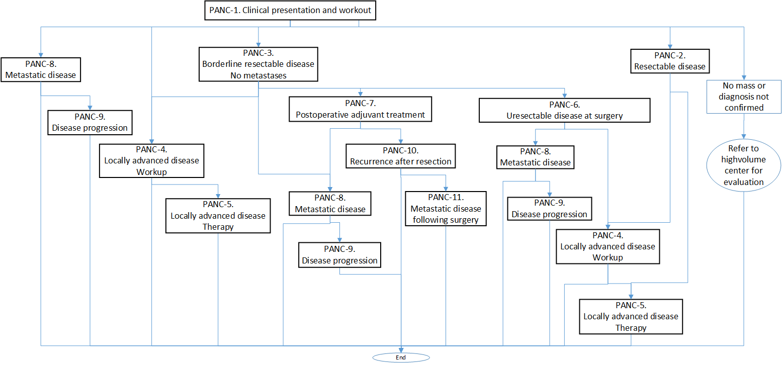
Figure 1: Calling scheme between the different processes (PANCs).

Algorithm 1 Clinical presentation and workup (PANC-1) [44].

- Clinical suspicion of pancreatic cancer or evidence of dilated pancreatic and/or bile duct (Indicators: age, gender)

- Pancreatic protocol CT (abdomen)

- Multidisciplinary consultation

if No metastatic disease then

     Medical tests:

     * Chest and pelvic CT

     * Consider endoscopic ultrasonography (EUS)

     * Consider MRI as clinically indicated for indeterminate liver lesions

     * Consider PET/CT in high-risk patients

     * Consider endoscopic retrograde cholangiopancreatography (ERCP) with stent placement

     * Liver function test and baseline CA 19-9 after adequate biliary drainage

     * Genetic testing for inherited mutations if diagnosis confirmed

     Possible outcomes:

     * Refer to high-volume center for evaluation

     * Resectable Disease, Treatment (Indicators: primary diagnosis, site of resection or biopsy)

     * Borderline Resectable Disease, No Metastases (Indicators: primary diagnosis, site of resection or biopsy)

     * Locally Advanced Disease (Indicators: primary diagnosis, site of resection or biopsy)

     * Metastatic Disease, First-Line Therapy, and Maintenance Therapy

else if Metastatic disease then

     Metastatic Disease

     Biopsy confirmation, from a metastatic site preferred

     Medical test:

     * Genetic testing form inherited mutations

     * Molecular profiling of tumor tissue is recommended

     * Complete staging with chest and pelvic CT

     Outcomes: (Indicators: primary diagnosis, site of resection or biopsy)

     * Metastatic Disease: First-Line and Maintenance Therapy

end if

Following this guideline we can observe in the procedure corresponding to the clinical presentation and workup the four main diagnostic groups that are used to establish the treatment to be followed and that correspond with the stages presented in the Cancer Staging subsection (2.2.1):

• Resectable disease. In this case the guidelines suggest proceeding with surgery (without neoadjuvant therapy), or EUS-guided biopsy if neoadjuvant therapy is considered and if not previously done, and consider stenting if clinically indicated.

• Borderline resectable disease. Here a EUS-guided biopsy is preferred (if not previously done), and a staging laparoscopy and Baseline CA is considered.

• Locally advanced disease. In this case a biopsy should be performed if not previously done, which may result in: a) cancer not confirmed, b) adenocarcinoma confirmed, and c) other cancer confirmed.

• Metastatic disease. Here the guidelines suggest: a) if jaundice present: placement of self-expanding metal stent, b) Genetic testing for inherited mutations, if not previously done, and c) Molecular profiling of tumor tissue, if not previously done.

In this context, it should be borne in mind that many of the diagnostic tests require a multidisciplinary consultation including an appropriate set of imaging studies, which implies that the diagnostic and treatment process is often subject to the heuristic knowledge of oncologists.

Algorithm 1 also shows a first approximation to the main indicators in the steps of the diagnosis and treatment process. In addition, after the interdisciplinary consultation, in the case of non-metastatic disease, the size and extent of the tumor (pathologic T), the number of nearby lymph nodes that are cancerous (pathologic N), the presence of metastases (pathologic M) and, from these, the pathological status are considered in the treatment of unresectable disease at surgery (for cases of resectable disease and borderline resectable disease), and in the treatment of locally advanced disease.

3 Data and methodology

3.1 Dataset

The dataset used in this work was obtained from The Cancer Genome Atlas Program [45], a joint effort between the USA National Cancer Institute (NCI) and the National Human Genome Research Institute. The Cancer Genome Atlas (TCGA) is a landmark cancer genomics program that sequenced and molecularly characterized over 11,000 cases of primary cancer samples.

One of the projects included in the program is called TCGA-PAAD, focused on pancreatic cancer, which provides 185 diagnosed cases with the necessary details to carry out its complete analysis. For example, it includes information such as: the “stage event” which describes the pathological state of the tumor, “clinical data” which describes the characteristics of the tumor, and the occurrence of “new tumor events” which describes the patient follow-up. We have only considered 181 cases since the remaining four were incomplete. From the 181 cases considered, 117 were applied a chemotherapy treatment. Each of the cases has a total of 158 features, ranging from family history data to treatment and follow-up information.

3.2 Feature selection

For our experiment we did a meticulous feature selection process in which only those features that added relevant information to the use case of whether to apply a chemotherapy treatment were selected [34].

As a first step, we analyze the dataset with all available information. Even if the data provided by the PAAD repository allows to upload many variables for each patient case, the projects that had collaborated with the institution did not provide all the information possible.

The second step was a pruning process performed over those features without information or with very few informed cases. We removed unnecessary data as the PAAD database includes many variables that do not intervene in the treatment decision process. Moreover, some information provided on the dataset was redundant, as for example the size of the tumor which can be inferred from the TNM diagnosis (as commented in section 2.2.1), so we eliminated the unnecessary data.

Finally, we asked a panel of oncologists, who participated as human experts, selecting only those features they considered relevant to treatment selection in pancreatic cancer patients. Our goal in including human experts in the feature selection process is to improve the explanatory power of the resulting models. As described in [46], they could also be involved with the aim of obtaining models with a higher accuracy.

After the expert selection and pruning process, we ended up with 27 features and the target variable which is the therapy type. From this group of features we created three different sets of features — recommended, maximum, and minimum — that would be used in the different ML models developed.

3.2.1 Recommended set

The inclusion of expert knowledge in the training of ML models can help to obtain better results and improve their interpretability. In this work, we first consider the collaboration of experts during the feature engineering process. We asked a panel of medical doctors to rate the relevance regarding the prescription of chemotherapy treatment, of the 27 features selected during the feature selection process. Each feature should receive a value between 1 and 3, being 1 highly relevant, 2 relevant, and 3 barely relevant.

From the results provided by the medical experts, we extracted a set of recommended features that includes those features that received a value of 1 or 2. Among the features selected by the experts, three of them were dependent on the treatment prescribed, so we also decided to remove them from the set as the objective is treatment prescription. They were namely the primary therapy outcome success, new tumor events, and days to new tumor event after the initial treatment. The details of the 14 features selected, the expert value received, and a brief description extracted from the GDC Data dictionary are shown in Table 1.

Table 1: Recommended set of features.

Feature	Experts	Description
Age	2	The patient’s age (in years).
Adenocarcinoma invasion	1	Confirm that the pancreas tumor sample being submitted to TCGA is an invasive adenocarcinoma.
Histological type	1	Indicate the histologic subtype, if available, for the pancreas adenocarcinoma tumor sample being submitted to TCGA.
Initial diagnosis method	2	Initial pathologic diagnosis method
Lymph nodes positive HE	1	Number of lymph nodes positive by Hematoxylin and Eosin (HE) Stain.
Maximum tumor dimension	1	Provide the length of the largest dimension/diameter of the original tumor as stated on the pathology report.
Neoplasm cancer status	2	The state or condition of an individual’s neoplasm at a particular point in time.
Neoplasm histologic grade	1	A description of a tumor based on how abnormal the cancer cells and tissue look under a microscope and how quickly the cancer cells are likely to grow and spread.
Pathologic stage	1	The extent of a cancer, especially whether the disease has spread from the original site to other parts of the body.
Pathologic N	2	Codes to represent the stage of cancer based on the nodes present.
Pathologic M	1	Code to represent the defined absence or presence of distant spread or metastases to locations via vascular channels or lymphatics beyond the regional lymph nodes.
Residual tumor	1	Text terms to describe the status of a tissue margin following surgical resection.
Surgery performed type	2	Indicate the type of surgical procedure performed.
Year of initial diagnosis	1	Year of initial diagnosis.

3.2.2 Maximum set

From this point, we explore two different options. On the one hand, we enhance the feature set adding all the available information gathered (i.e., all 27 features). Even if some features were “barely relevant” for medical doctors, there are studies in which some evidence is assigned to them as risk factors for pancreatic cancer, as it is the case of gender, race, or ethnicity [47, 48]. We named the complete set of features as the maximum set.

The idea behind this was to retain all the information available for the development of the ML models, so they can detect complex relationships among the features and ultimately produce a robust model. Therefore, we added 13 more features to our recommended set (shown in Table 2) ending up with the complete feature set.

Table 2: Features added to the maximum set (jointly with those presented in Table 1).

Feature	Expert	Description
Alcoholic exposure category		Indicate the patient’s current level of exposure to alcohol.
Days to new tumor after treatment	1	Days to new tumor after initial treatment.
Family history of cancer	3	Indicate if a first degree relative (parents, siblings, or children) of the patient has a history of a cancer diagnosis.
Ethnicity		An individual’s self-described social and cultural grouping, specifically whether an individual describes themselves as Hispanic or Latino.
Gender		Text designations that identify gender. Gender is described as the assemblage of properties that distinguish people on the basis of their societal roles.
History of diabetes	3	Indicate if the patient has been previously diagnosed with diabetes.
New tumor events	1	Indicate whether a new tumor event occurs.
Other DX		Numeric value to express the degree of abnormality of cancer cells, a measure of differentiation and aggressiveness.
Pathologic T	3	Code of pathological T (primary tumor) to define the size or contiguous extension of the primary tumor (T).
Primary therapy outcome success	1	Indicates a complete remission or response to the prescribed treatment.
Race		An arbitrary classification of a taxonomic group that is a division of a species. It usually arises as a consequence of geographical isolation within a species and is characterized by shared heredity, physical attributes and behavior, and in the case of humans, by common history, nationality, or geographic distribution.
Radiation therapy		Whether the treatment includes a radiation therapy.
Tobacco smoking history		Category describing current smoking status and smoking history as self-reported by a patient.

3.2.3 Minimum set

The other option chosen was to reduce the dimensionality of the dataset as the staging TNM variables implicitly include valuable information about the status of the cancer (see section 2.2.1). It is the case for example of the pathologic T that informs about the size of the tumor, or the pathologic M that indicates if a metastasis has occurred. Therefore, we considered the minimum set of features as a dimensionality reduction with the goal of transforming high-dimensional data into a lower-dimensional representation without losing any important information. We ended up with five features (Age, T, N, M and Stage) that we can see in Table 3 along their range of values.

Table 3: Minimum set with the range of values.

Age	T	N	M	Stage
35-88	TX T1 T2 T3 T4	N0 N1 N1b NX	M0 M1 MX	Stage 0 Stage I, IA, IB Stage II, IIA, IIB Stage III Stage IV

3.2.4 Features and guidelines

As a final step to evaluate feature importance we decided to follow the medical guidelines from the “Pancreatic Adenocarcinoma - NCCN Clinical Practice Guidelines in Oncology” [44] to see how they consider each feature in terms of importance. As we have seen in Figure 1 and Algorithm 1, these guidelines are quite complex and detail the sequential management decisions and interventions regarding pancreatic cancer, providing recommendations for some of the key issues in cancer prevention, screening, and care.

Therefore, feature importance regarding the chemotherapy treatment is not clearly specified in those guidelines so it is necessary to carry out a process of knowledge elicitation that allows us to extract such information. For this purpose, we analyzed the different procedural sheets into which the guideline is divided, taking into account that the same sheet can be considered in different diagnostic lines. This implies that successive tests may involve refinements or changes in determining the diagnosis and treatments to be used.

The final result of this analysis is presented in Figure 2 in which we show the decisions that we have to take leading to a chemotherapy treatment. It is important to remark that this figure is a simplification to highlight the fundamental decisions and considerations involved in chemotherapy treatment, and that the complete diagnostic process is more complex.

Figure 2: Simplified graph of diagnostic decisions involving chemotherapy treatment.

Each of the nodes represent an evaluation that we have roughly mapped onto a feature value, so that we can follow the diagnosis path. We could use the staging M as an evaluation of Metastatic disease, the size of the tumor T to determine whether it is resectable or not, and the N to evaluate if the cancer is locally advanced or not.

In Table 4 we can see the set of maximum features ranked by the medical experts, as commented before, but also ranked using the information extracted from the medical guidelines.

Table 4: Feature importance from the expert criteria and medical guidelines.

Abbr.	Feature	Guidelines	Experts
Age	Age	3	2
Stage	Stage	1	1
T	T	2	3
N	N	2	2
M	M	2	1
Year	Year of initial diagnosis	3	1
Adeno.	Adenocarcinoma invasion	2	1
Type	Histological type	2	1
Status	Neoplasm cancer status	1	2
Grade	Neoplasm histologic grade	3	1
Dimensi.	Maximum tumor Dimension	1	1
Residual	Residual tumor	3	1
Diagnos.	Initial diagnosis method	2	2
Surgery	Surgery performed type	2	2
Lymph	Lymph nodes positive by HE	1	1
Gender	Gender
Race	Race
Ethnic.	Ethnicity
Other	Other DX
Diabetes	History of diabetes	3	3
Family	Family history of cancer	2	3
Radiat.	Radiation therapy	2	2
Therapy	Therapy outcome success	2	1
N. tumor	New tumor events		1
Days to	Days to new tumor		1
Tobacco	Tobacco smoking history
Alcohol	Alcoholic exposure category

3.3 Machine learning models

With the aim of comparing different models in terms of accuracy and understandability, we chose three types of ML models: a Decision Tree, a Random Forest and an XGBoost. All of them are tree-based algorithms that are known to be easily understandable, but as they increase in complexity they require to be enhanced with ad-hoc exaplainability methods to be able to interpret their results. We do include a brief description of all of them highlighting the advantages and disadvantages in terms of accuracy and understandability.

As a general rule, when efficiency improvement is needed, aggregation techniques as bagging or bootstrapping are applied.

• Bagging, also known as bootstrap aggregation, is the ensemble learning method that is commonly used to reduce variance within a noisy data set by combining the prediction of single models using various aggregation techniques.

• Bootstrapping is a technique used to iteratively improve a classifier’s performance. Typically, multiple classifiers will be trained on different sets of the input data, and on prediction tasks the output of the different classifiers will be combined.

These methods are based on tree ensembles, which combine different single trees to obtain an aggregated prediction. Although the results are usually more efficient and mitigate overfitting, the interpretation of these models is far more complex.

3.3.1 Decision trees

A Decision Tree (DT) is a non-parametric supervised learning algorithm, which is used for both classification and regression tasks. It has a hierarchical tree structure, which consists of a root node, branches, internal nodes and leaf nodes [49].

DTs offer advantages over other AI models as they are easy to interpret. They do not require advance knowledge on AI to understand how they are built as they are a common structure used in many other fields. They allow a graphical representation of the algorithm, which makes them a perfect candidate in scenarios where understandability is key. Another significant advantage in these models is that they require a minimum set of data and the features are directly included in the model. The calculations required to get the a decision are also simple and easy to understand. They can handle both numerical and categorical data, and inherently perform feature selection.

Nevertheless, they can produce overfitting, not generalizing competently when fed with new data. They are also sensitive to small changes in the input data, so small variations can generate very different trees. And finally, they are not good at discovering complex relationships between features.

To overcome these issues, simple models can be combined to get an aggregated model. However, and as usual, increasing the complexity of the model makes it harder to understand. Therefore, to be able to explain the decisions performed by the model, and infer which are the most relevant features taken into consideration, a complementary method is required.

3.3.2 Random Forests

Random Forests (RFs) are the result of combining a set of DTs forming ensembles. Each DT output is combined to reach a single result [7]. It operates by constructing a multitude of decision trees during the training phase and outputs the mode of the classes of the individual trees.

The main advantages of the RFs include high accuracy, robustness to overfitting, and the capacity to handle large datasets. In terms of understandability, they provide a way to measure the feature importance. Another great advantage is that RFs do not make assumptions about the distribution of the data and are able to capture complex relationships between features and the target variable. They scale in both number of features or observations, and their computation could be parallelized to get faster training times.

In simple scenarios, due to the complexity of the structure, it requires more computation than single trees, and its interpretability decrease. Even though the algorithm required to compute predictions can be parallelized, they are computationally intensive and consume more memory than individual decision trees.

3.3.3 XGBoost

XGBoost stands for “eXtreme Gradient Boosting” and it is built combining many simple models to create an ensemble with higher prediction capabilities [50]. It is made up of a series of weak learners (typically decision trees) sequentially, with each new model attempting to correct the errors made by the previous ones and uses a gradient-based optimization algorithm to construct the trees, with the objective of minimizing a user-defined loss function.

XGBoost is one of the most efficient models in terms of accuracy and it can be applied over datasets where both categorical and numeric features are included. It often outperforms RF in terms of predictive accuracy, especially when dealing with structured/tabular data. While RF has some mechanism to mitigate overfitting, XGBoost incorporates regularization, which provides better control.

On the other hand, the interpretability of the resulting models is far more complicated than a single tree and it requires specific knowledge to be able to tune its parameters. While both XGBoost and RF are ensemble models, RF models are often considered more interpretable than XGBoost due to their simpler structure.

3.4 Explainability models

Explainability models or techniques are used to enhance the interpretability and understanding of ML models, helping the users to understand and interpret the decisions made by these models.

In this work we focused on using Feature Importance [51] as an explainability method. Feature importance refers to a class of techniques for assigning scores to input features of a predictive model that indicates the relative importance of each feature when making a prediction.

We have included two model-specific explainability methods for tree-based models and two model-agnostic explainability methods, which we will briefly explain in the next sections.

3.4.1 Model-specific methods

Feature importance scores for tree-based models can be broadly split into two categories [52]:

• Split-improvement scores that are specific to tree-based methods and that naturally aggregate the improvement associated with each node split and can be readily recorded within the tree building process.

• Permutation methods that rely on measuring the change in value or accuracy when the values of one feature are replaced by uninformative noise, often generated by a permutation.

Mean Decrease in Impurity (MDI)

Mean Decrease in Impurity (MDI) is a split-improvement score that measures the inherent importance of different measures [7]. This is determined by how much each feature contributes to reducing the uncertainty in the target variable. MDI is measured by the amount of reduction in the Gini impurity or entropy that is achieved by splitting on a particular feature.

Mean Decrease Accuracy (MDA)

Mean Decrease Accuracy (MDA) (also known as “Permutation Importance”) [7] measures how the accuracy score decreases when a feature is not available. It randomly discards each feature and computes the change in the performance of the model, and orders them based on their impact.

3.4.2 Model-agnostic Methods

As commented, model-agnostic explainability methods are independent of the specific ML model used and can be applied to any model, regardless of its architecture or underlying algorithms.

SHapley Additive exPlanations (SHAP)

Presented by Lundberg and Lee [53], SHAP (SHapley Additive exPlanations) is a unified framework for interpreting predictions. It is model-agnostic method that assigns each feature an importance value for a particular prediction. Its origins are related to the cooperative game theory where players collaborate together to obtain a certain score. In the AI scenario, the players are the features and the score is the prediction.

At a general level, SHAP gives us the insights about the weight of each of the features involved in the classification process. The SHAP framework allows for a practical visualization of the Shapley value using an “importance” diagram.

We are then interested in the contribution of each of the features to the final decision, which is calculated by the SHAP value.

Locally Interpretable Model-agnostic Explanations (LIME)

Proposed by Ribeiro et. al [54], Locally Interpretable Model-agnostic Explanations (LIME) tries to understand the features that influence a prediction on a single instance. It focuses on a local level where a linear model is enough to explain the model behavior. LIME creates a surrogate model around the example for which we try to understand the prediction made.

Its scope is inherently local, therefore, in order to compare the results of LIME at a global level, it is necessary to iterate over all the examples and gather the most frequent features in terms of importance.

4 Results

In this section we will present the results of the different ML models in terms of accuracy and interpretability given the three feature sets discussed in section 3.2 and compare them with the medical guidelines and the medical criteria used as reference.

4.1 Accuracy of the resulting models

As the basis for the evaluation of accuracy of the different models included in this experiment we have used the following metrics:

• Accuracy that shows how often a classification ML model is correct overall.

• Precision that shows how often an ML model is correct when predicting the target class.

• Recall that shows whether an ML model can find all objects of the target class.

• F1 Score that provides a balance between precision and recall, making it a more comprehensive metric for evaluating classification models.

In our specific scenario with a dataset unbalanced to chemotherapy cases, the F1-score provides a more robust metric. The model parameters (e.g., max depth, min samples per leaf, etc.) have been established by selecting the optimal configuration in every case. Each model was evaluated using different configurations, and we did only keep the one with higher accuracy. Results can be seen in Table 5.

Table 5: Accuracy results for three ML models using three different feature sets.

Model	Parameters	Feature Set	Accuracy	Precision	Recall	F1-Score
DT	md=3, msl=5	Minimum	0,66	0,72	0,66	0,63
DT	md=2, msl=30	Recommended	0,57	0,58	0,57	0,55
DT	md=3, msl=20	Maximum	0,62	0,62	0,62	0,62
RF	md=2, msl=5	Minimum	0,54	0,76	0,54	0,43
RF	md=3, msl=5	Recommended	0,51	0,76	0,51	0,38
RF	md=4, msl=5	Maximum	0,51	0,76	0,51	0,38
XGB	md=2, ne=50	Minimum	0,66	0,70	0,66	0,64
XGB	md=4, ne=40	Recommended	0,54	0,53	0,54	0,52
XGB	md=3, ne=40	Maximum	0,59	0,62	0,59	0,55

From Table 5 we can state that the best models in terms of accuracy have been those models built with the minimum set of features. This circumstance suggest that adding additional information to a dataset does not always result in better accuracy, and moreover it makes the models more complex.

Referring to the type of the models, DTs are more accurate in general but their results are very close to those produced by the XGBoost. The intuition we had when using an advanced type of model, such as XGBoost, was that the increased complexity would translate into improved performance. The fact of not having any gain in accuracy could be explained by the small size of the training set, as it is known that typically ML algorithms require a big amount of data to produce acceptable results.

4.2 Interpretability of the resulting models

Presenting interpretability information is a bit complex, since there is no defined measure of how correct the interpretation of an ML model is. We intend to move in this direction by comparing the interpretability of the models with what the medical criteria of the field expressed through guidelines and the opinion of the physicians. In the following sections we will discuss how to analyze the importance of the different features according to the different explainability methods used for the different feature sets.

4.2.1 Extracting the feature importance from XAI methods

In this section we will illustrate how to extract the feature importance that the XAI methods assign to the different features given a ML model. To this end we chose a DT model (since it is transparent regarding interpretability) trained with the minimum set of features (to make the figures more readable). The DT parameters that obtain the best accuracy are 3 as the maximum depth of the tree, 5 as the minimum samples per leaf, and Gini as the split criterion. The best accuracy obtained was approximately 0.66.

Figure 3 shows the DT obtained. In this figure we can observe that pathologic N, pathologic stage and age are the most relevant features. In the following sections we will apply different explainability methods and extract the feature importance delivered by them.

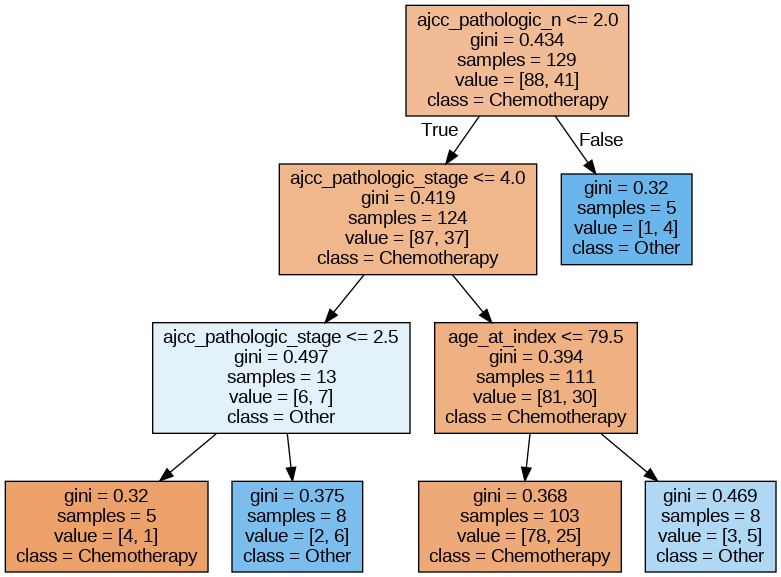
Figure 3: Decision tree for the minimum set of features.

Using MDI to examine the feature importance of the classifier using the minimum feature set, we obtain the results of Figure 4. The size of each bar is related to the relevance of the feature. So, in this case, stage is the most relevant feature followed by pathologic N and age.

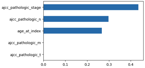
Figure 4: MDI for the DT with the minimum set of features.

On the other hand, using MDA to examine the feature importance of the classifier using the minimum feature set, we obtain the results of Figure 5. Here, relevant features are highlighted. In this case, stage is the most relevant feature followed by age.

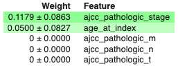
Figure 5: MDA for the DT with the minimum set of features.

Taking into account the model-agnostic method SHAP, Figure 6 presents the feature importance of the classifier using the minimum feature set. This figure is the summary chart of SHAP which presents in the left axis the features in order of relevance. In this case, stage, age and pathologic N the most important ones.

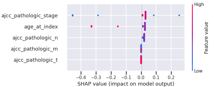
Figure 6: SHAP for the DT with the minimum set of features.

Finally, LIME was applied to the same configuration. In Figure 7 we show the local explanation of a particular patient that indicates stage, pathologic T and pathologic N as the most important features. Nevertheless, to be able to evaluate and compare LIME results at a global level we iterate over all the local explanations and keep the most frequent features for all the examples. Stage, pathologic N and age are the most relevant features at a global level.

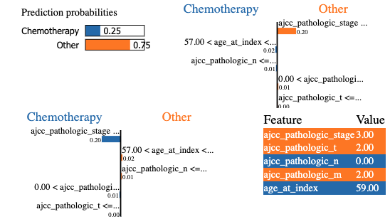
Figure 7: LIME for the DT with the minimum set of features for the different ML models and XAI methods.

All these results for the DT classifier using the minimum feature set are summarized in Table 6 assigning a “1” to the highly relevant features, “2” for relevant features and “3” for the less relevant. Leaving blank values if the feature is not relevant for the XAI method. We also include for comparison the relevance of the features using the medical guidelines and the medical expert criteria.

Table 6: Feature importance for the minimum set of features.

	DT				RF				XGB
Feature	MDI	MDA	SHAP	LIME	MDI	MDA	SHAP	LIME	MDI	MDA	SHAP	LIME	Guid.	Exp.
Age	2	2	1	3	1	3	2	3	2	1	1	2	3	2
Stage	1	1	1	1	1	1	1	1	1	1	1	1	1	1
T					3	3	3		2	3	2	2	2	3
N	2		3	3	2	1	2	1	2	2	3		2	2
M					3		2	3	2	2	2	2	2	1

4.2.2 Similarity index

We need a metric that allows us to compare the results obtained. One good candidate is the Jaccard Similarity index [55] that measures the similarity between two sets dividing the size of the intersection by the size of the union of the two sets. Mathematically, given two finite sets $S$ and $T$ from a universe $U$, the Jaccard similarity of $S$ and $T$ is defined as:

$$jacc(S,T)=\frac{|S\cap T|}{|S\cup T|}$$

In our case the elements of the set are the different features and the importance that the different models of explainability give to these features. In addition, we not only want to see if the elements of the different sets coincide, we also want to see if they coincide in order, giving more importance to the coincidences in the first positions. For that reason the Weighted Jaccard Similarity index [55] is more convenient since it allows to handle cases where elements in the data have different weights or importance.

The Weighted Jaccard Similarity index assumes that a weighted set exists that associates a real weight to each element in it (being this weight $\geq 0$). Therefore a weighted set is defined by a map $w:U\rightarrow\mathbb{R}$. In our case, since we want to give more importance to the first position matches we assign a weight of $3$ to the first position, $2$ to the second position, $1$ for the third position and $0$ for the non-ranked elements.

Thus, given two vectors of weights $\mathbf{x}=(x_{1},x_{2},\ldots,x_{n})$ and $\mathbf{y}=(y_{1},y_{2},\ldots,y_{n})$ with all real $x_{i},y_{i}\geq 0$, then their weighted Jaccard similarity coefficient is defined as:

$$J_{\mathcal{W}}(\mathbf{x},\mathbf{y})=\frac{\sum_{i}\min(x_{i},y_{i})}{\sum_{i}\max(x_{i},y_{i})}$$

In Table 7 and Table 8 we can see the results of calculating the weighted Jaccard index for the DT and XGB models respectively according to the data included in Table 6. We decided to focus our analysis in the two models that offer the best performance.

Table 7: Similarity measures for the different XAI methods using the DT model and the minimum set of features.

	MDI-DT	MDA-DT	SHAP-DT	LIME-DT	Guidelines	Experts
MDI-DT	1.00	0.71	0.75	0.71	0.55	0.64
MDA-DT	0.71	1.00	0.71	0.67	0.36	0.45
SHAP-DT	0.75	0.71	1.00	0.71	0.42	0.50
LIME-DT	0.71	0.67	0.71	1.00	0.50	0.45
Guidelines	0.55	0.36	0.42	0.50	1.00	0.75
Experts	0.64	0.45	0.50	0.45	0.75	1.00

Table 8: Similarity measures for the different XAI methods using the XGB model and the minimum set of features.

	MDI-XGB	MDA-XGB	SHAP-XGB	LIME-XGB	Guidelines	Experts
MDI-XGB	1.00	0.83	0.83	0.81	0.91	0.83
MDA-XGB	0.83	1.00	0.83	0.67	0.75	0.83
SHAP-XGB	0.83	0.83	1.00	0.82	0.75	0.69
LIME-XGB	0.81	0.67	0.82	1.00	0.73	0.67
Guidelines	0.91	0.75	0.75	0.73	1.00	0.75
Experts	0.83	0.83	0.69	0.67	0.75	1.00

From these tables we can see several things, firstly that the degree of similarity between the guides and the experts is high (0.75), and the same occurs between the different methods of explainability. We see that the main similarity is that they all agree in assigning the stage as the most important feature, while the main difference is that the ML models give less importance to features such as T and M.

4.2.3 Feature importance using the recommended feature set

In this section we will present the interpretability results for each ML model and each feature relevance method using the recommended features set. The results are summarized in Table 9.

Table 9: Feature importance for the recommended set of features.

	DT				RF				XGB
Feature	MDI	MDA	SHAP	LIME	MDI	MDA	SHAP	LIME	MDI	MDA	SHAP	LIME	Guid.	Exp.
Age	1	2	1		1	3	2		1	2	1	2	3	2
Stage	2	1	2	1	1	1	1	1	1	2	2	1	1	1
N					2	1	2	3	2		3		2	2
M					2	2	3		3		3		2	1
Year	2	1	1	2	1	1	1	3	2			1	3	2
Adeno.													2	2
Type					2	1	2		1	1	3		2	1
Status	2	2	1	1	3	1	3		1	2	2		1	1
Grade					2	2	2		2	1	3		3	3
Dimensi.	3		3		2	1	3		2		2		1	1
Residual	1		2	2	2		1	1	2		1	1	3	1
Diagnos.					3	1	3		1	1	2		2	2
Surgery					3	1	2		3				2	2
Lymph					2	1	2		2		2		1	1

In Table 10 and Table 11 we can see the similarity results for the DT and XGB models respectively according to the data included in Table 9. From these two tables we can see that again there is a high similarity between experts and guides, and that the similarity between the XAI methods is quite consistent (except for LIME).

Table 10: Similarity measures for the different XAI methods using the DT model and the recommended set of features.

	MDI-DT	MDA-DT	SHAP-DT	LIME-DT	Guidelines	Experts
MDI-DT	1.00	0.53	0.80	0.53	0.24	0.34
MDA-DT	0.53	1.00	0.60	0.54	0.23	0.26
SHAP-DT	0.80	0.60	1.00	0.60	0.27	0.33
LIME-DT	0.53	0.54	0.60	1.00	0.27	0.29
Guidelines	0.24	0.23	0.27	0.27	1.00	0.82
Experts	0.34	0.26	0.33	0.29	0.82	1.00

Table 11: Similarity measures for the different XAI methods using the XGB model and the recommended set of features.

	MDI-XGB	MDA-XGB	SHAP-XGB	LIME-XGB	Guidelines	Experts
MDI-XGB	1.00	0.47	0.68	0.28	0.63	0.70
MDA-XGB	0.47	1.00	0.35	0.21	0.30	0.32
SHAP-XGB	0.68	0.35	1.00	0.29	0.50	0.58
LIME-XGB	0.28	0.21	0.29	1.00	0.20	0.24
Guidelines	0.63	0.30	0.50	0.20	1.00	0.82
Experts	0.70	0.32	0.58	0.24	0.82	1.00

If we focus on the DT data we can see that the decision trees take into consideration fewer features than the experts and the guides, which is normal since they only consider those that are necessary to establish a decision. This results in low similarity values. On the other hand the XGB model spreads the importance along the different measures, therefore the similarity values with experts and guides are higher. we see that the features chosen as the important ones by the DT model and according to the XAI methods are: Age, Stage, Year of initial diagnosis, Neoplasm cancer status and Residual tumor. Except for Age and Year the rest are considered very or fairly important by experts and guides. On the other hand, XGB considers again features such as Age, Stage, Residual tumor or Neoplasm cancer status. But the biggest difference is that it considers features that are completely irrelevant for the DTs but relevant for experts and guides such as Histological type or Initial diagnosis method.

4.2.4 Feature importance using the maximum feature set

In this section the interpretability results for each ML model and each features relevance method using the maximum features set is presented. Table 12 summarize the results.

Table 12: Feature importance for the maximum set of features.

	DT				RF				XGB
Feature	MDI	MDA	SHAP	LIME	MDI	MDA	SHAP	LIME	MDI	MDA	SHAP	LIME	Guid.	Exp.
Age	3	2	3		1		2	2	1		1	2	3	2
Stage	2	2	1	2	1	1	1	1	2	1	1	1	1	1
T					2	2	3						2	3
N					2	1	2	3	3				2	2
M					3	2	3		3				2	1
Year	1	1	1		1	3	1	3	2		1	3	3	1
Adeno.							3						2	1
Type				3	2	1	3		3	1	2		2	1
Status					3		3		3		2		1	2
Grade					2	2	3		3	2	3		3	1
Dimensi.					1		3		1	3	2		1	1
Residual					2		1	2	3	2	1		3	1
Diagnos.					3		3		3		2		2	2
Surgery					3		3						2	2
Lymph					2	3	3		2		2		1	1
Gender					2				2	1	1
Race					2		2	2	3		3	3
Ethnic.					3		3				3
Other DX					3		3
Diabetes					2		3		3				3	3
Family	2		1	1	2	2	2		3	1	1	1	2	3
Radiat.					2	3	3		3	2	3		2	2
Therapy					3		2		3		3		2	1
N.tumor					3		3			2				1
Days to					2				3					1
Tobacco					2	3	3		2		2
Alcohol					2				3		2

In Table 13 and Table 14 we can see the similarity results for the DT and XGB models respectively according to the data included in Table 12. As there are more features, the similarity values decrease, which is to some extent normal since the ambiguity inherent in assigning concrete values of importance to the different measures must be taken into account.

Table 13: Similarity measures for the different XAI methods using the DT model and the maximum set of features.

	MDI-DT	MDA-DT	SHAP-DT	LIME-DT	Guidelines	Experts
MDI-DT	1.00	0.67	0.80	0.40	0.15	0.13
MDA-DT	0.67	1.00	0.55	0.18	0.10	0.14
SHAP-DT	0.80	0.55	1.00	0.45	0.18	0.15
LIME-DT	0.40	0.18	0.45	1.00	0.13	0.08
Guidelines	0.15	0.10	0.18	0.13	1.00	0.63
Experts	0.13	0.14	0.15	0.08	0.63	1.00

Table 14: Similarity measures for the different XAI methods using the XGB model and the maximum set of features.

	MDI-XGB	MDA-XGB	SHAP-XGB	LIME-XGB	Guidelines	Experts
MDI-XGB	1.00	0.24	0.60	0.26	0.43	0.40
MDA-XGB	0.24	1.00	0.38	0.26	0.26	0.29
SHAP-XGB	0.60	0.38	1.00	0.35	0.40	0.40
LIME-XGB	0.26	0.26	0.35	1.00	0.19	0.18
Guidelines	0.43	0.26	0.40	0.19	1.00	0.63
Experts	0.40	0.29	0.40	0.18	0.63	1.00

From these tables we can see that in DT the results of the XAI methods are quite consistent with each other, highlighting few features but almost always the same (Age, Stage, Year, Family history). XGB takes into account the influence of more features but the explanatory methods are not as consistent with each other, indicating that it is a more opaque model from which it is more difficult to find consistent explanatory measures.

5 Discussion

Performance

Regarding the performance of the different ML models, as described throughout the results section, the accuracy obtained is low; all of them present similar accuracy values near, but not reaching 0.7. There is a justification for such low precision values and, in any case, they are not entirely relevant to the objective we are pursuing in the paper. First of all, we can say that the dataset has few cases, so ML models suffer when trying to generalize patterns present in the data. This is a clear data bottleneck problem and, as discussed in [46], a possible solution is to use data augmentation strategies to improve data quality and quantity. In that work the accuracy increased more than 10 percent with the collaboration of human experts who helped to improve the labeling and the generation of synthetic cases.

However, the aim of this paper was to focus on how to evaluate the explanatory capabilities of ML models and to analyze the consistency between different XAI methods. Adding synthetic data could improve accuracy but at the cost of introducing correlations that might not be real and could affect explanatory capabilities.

Comparing the different ML models, we can see that DT and XGBoost models deliver similar results in terms of accuracy in all scenarios. The fact of increasing or decreasing the set of features did not make the RF model nor the XGBoost model better in terms of performance. It could be due to the small number of examples used to train the model. Normally, they are expected to find complex relationships between the different features but in our work it was not the case. Although all ML models are tree-based and that bagging and boosting techniques are included in the RF and XGBoost models respectively, we have found no gain in terms of accuracy nor in explicability matters.

Regarding the different features sets used, it is interesting to highlight that the minimum feature set was the one that obtained better results in terms of accuracy. One possible explanation could be the type of features included in this set. Apart from age, features like pathologic T (code to define the size or contiguous extension of the primary tumor), pathologic N (code to represent the stage of cancer based on the nodes present), pathologic M (code to represent the defined absence or presence of distant spread or metastases to locations via vascular channels or lymphatics beyond the regional lymph nodes) and stage (code to represent the extent of a cancer, especially whether the disease has spread from the original site to other parts of the body) are summarizing codes of the cancer status. Therefore, they are a sort of dimensionality-reduction technique applied by physicians to better understand and communicate cancer status. In these features is included much of the information needed to decide whether to give chemotherapy treatment although, obviously, the detailed treatment itself requires more information. The remaining sets of features offer lower results, but very close to the results of the minimum feature set.

Human-in-the-Loop

The participation of humans in the process of developing ML systems (a.k.a., Human-in-the-loop or HITL) could help in enhancing transparency, improving trust, and achieving better performance [56]. Nowadays, there exist many tools supporting the inclusion of human experts both as ML practitioners or as domain experts [57].

Regarding Feature Engineering (FE) we have seen that it is an important part of every ML project. There have been other works that focus in HITL feature engineering process. For example, Anderson et al. [58] propose an interactive HITL FE scheme, based on state-of-the-art dimensionality reduction for nowcasting features for economic and social science models; and Gkorou et al. [59] propose an interactive FE scheme based on dimensionality reduction for Integrated Circuit (IC) manufacturing. Both cases show that by engineering features it is possible to obtain higher predictive capabilities and to improve the interpretability of the model.

In our case we collaborate with medical experts for: 1) selecting the best features available from the specialized dataset and, 2) establishing a relevance value creating a recommended set of features and giving insights about the pancreatic cancer diagnosis. This collaboration required an active participation of human experts, something that add complexity to the process.

But we also have use medical expertise through medical guidelines, that are standard procedures in the field. This process of analyzing medical guidelines do not require the active participation of human experts but have also its complexities as this guidelines tend to be exhaustive and sometimes hard to navigate through.

This collaboration with human experts of the domain and the analysis of guidelines available in the same domain can be used not only as a feature engineering process, but also as a way to evaluate explainability methods.

Explainability

When it comes to explainability, it is important to notice that each approach available measure specific responses of the model using different techniques, and thus they could produce different results. However, in this work we have been able to see that, as a general rule, the explanatory methods, given a given ML model, provide fairly consistent results among themselves, with high levels of similarity.

We can see that, methods such as MDI and SHAP use very different procedures to reach their conclusions, but they are very similar in terms of feature importance. Also SHAP provides several charts that allow us to better understand the explainability results and it has also the advantage of being model-agnostic, so that we can compare the results over different ML models.

In any case, we should not expect these tools on their on to produce human understanding of the models. Normally, they require a thoughtful interpretation to understand the underlying decision making process. Furthermore, explainability of black-box models have been criticized because the explanations either do not provide enough detail to understand what the black-box is doing or even they do not make sense [60].

To try to facilitate the interpretation of these explanatory results, we use a similarity measure such as the Weighted Jaccard Similarity coefficient. From their results we can see several things: Firstly, models like DT are more “decisive” when it comes to giving importance to features, for this ML model only a few features are important for the final result. On the other hand, and due to the very nature of the model, XGB distributes this importance more evenly among the different features. This has an effect on our results, as guides and experts also distribute the importance among the different features the similarity index of XGB with experts and guides is usually higher than that of DT.

We could say then that this behavior of XGB is more “human”, since it tries to take more information into account when making a decision. Although in this case taking into account more features does not correspond to a better performance, this may be due to problems inherent to the dataset itself and its low number of cases. Thus, for example, we see that the DT model eliminates from its consideration features such as Histological type or Initial diagnosis that are taken into account by experts and guides. A model such as XGB does take them into account.

Regarding the importance given by the experts and the guides to the different features, we can see that the similarity index between them is always high, with some variations that are easy to explain by the subjectivity of the assignment of values.

Regarding how the models assign importance to the features in comparison with guidelines and experts, in general we can say that the features pointed out as relevant by physicians and guidelines have been taken into account by the models but with some notable exceptions. Thus, for example, staging M has been generally forgotten by ML models when physicians assigned it a high importance. On the other hand, we have also observed that some features with low relevance for the experts, are considered by the XAI methods, such as, for example the Year of initial diagnosis.

6 Conclusions

As final conclusions we can highlight that, in this last “spring” of AI, researchers have decided to leave symbolic AI aside because its results were not entirely good and these AI models were very difficult to scale to larger problems. However, by embracing ML and subsymbolic AI we are getting better results, but these results have a worse interpretability because they have lost that symbolic character.

By trying to analyze ML results and compare their explainability through information from domain experts and guides what we are trying to do is to give “symbolism” to these results, to try to understand them from a human point of view. This approach is not problem-free, it requires active collaboration on the part of physicians, and medical guidelines are complex documents that require time for analysis.

However, we believe that the similarity measures used to analyze the importance of the different features can be an interesting way to evaluate explainability methods. The fact that the best models are the most opaque may cause such models to be discarded in critical domains such as health. Explainability agnostic methods and similarity measures can be used as techniques to better understand how the model works and whether the model adheres to recommended medical practices.

Until now, the feature importance was used as a measure of dimensionality reduction, allowing to simplify the problem being modeled in order to try to speed up the learning process and, in some cases, to improve the performance of the ML model. In our case what we intend to do is to use the feature importance as a way of evaluating the explainability of the different models.

As future work we plan to further develop the field of explainability metrics, we believe that in the future this type of metrics will be as common as performance metrics (accuracy, F1-score) are today. The idea is not only to choose the model that offers the best performance, but also the model that can best explain its conclusions and whose reasoning is best aligned with human knowledge of the domain.

Acknowledgements

This work has been supported by the State Research Agency of the Spanish Government (Grant PID2019-107194GB-I00/AEI/10.13039/501100011033) and by the Xunta de Galicia (Grant ED431C 2022/44), supported by the EU European Regional Development Fund (ERDF). We wish to acknowledge support received from the Centro de Investigación de Galicia CITIC, funded by the Xunta de Galicia and ERDF (Grant ED431G 2019/01). The results published here are in whole or part based upon data generated by the TCGA Research Network: https://www.cancer.gov/tcga

References

- \bibcommenthead
- Linardatos et al. [2021] Linardatos, P., Papastefanopoulos, V., Kotsiantis, S.: Explainable ai: A review of machine learning interpretability methods. Entropy 23(1) (2021) https://doi.org/10.3390/e23010018
- Angelov et al. [2021] Angelov, P.P., Soares, E.A., Jiang, R., Arnold, N.I., Atkinson, P.M.: Explainable artificial intelligence: an analytical review. Wiley Interdisciplinary Reviews: Data Mining and Knowledge Discovery 11(5), 1424 (2021)
- Barredo Arrieta et al. [2020] Barredo Arrieta, A., Díaz-Rodríguez, N., Del Ser, J., Bennetot, A., Tabik, S., Barbado, A., Garcia, S., Gil-Lopez, S., Molina, D., Benjamins, R., Chatila, R., Herrera, F.: Explainable artificial intelligence (xai): Concepts, taxonomies, opportunities and challenges toward responsible ai. Information Fusion 58, 82–115 (2020) https://doi.org/10.1016/j.inffus.2019.12.012
- Montavon et al. [2018] Montavon, G., Samek, W., Müller, K.-R.: Methods for interpreting and understanding deep neural networks. Digital Signal Processing 73, 1–15 (2018) https://doi.org/10.1016/j.dsp.2017.10.011
- Slack et al. [2021] Slack, D., Hilgard, A., Singh, S., Lakkaraju, H.: Reliable post hoc explanations: Modeling uncertainty in explainability. In: Ranzato, M., Beygelzimer, A., Dauphin, Y., Liang, P.S., Vaughan, J.W. (eds.) Advances in Neural Information Processing Systems, vol. 34, pp. 9391–9404. Curran Associates, Inc., Virtual conference (2021). https://proceedings.neurips.cc/paper_files/paper/2021/file/4e246a381baf2ce038b3b0f82c7d6fb4-Paper.pdf
- Kotsiantis [2013] Kotsiantis, S.B.: Decision trees: a recent overview. Artificial Intelligence Review 39(4), 261–283 (2013) https://doi.org/10.1007/s10462-011-9272-4
- Breiman [2001] Breiman, L.: Random forests. Machine learning 45, 5–32 (2001) https://doi.org/10.1023/A:1010933404324
- Chen and Guestrin [2016] Chen, T., Guestrin, C.: Xgboost: A scalable tree boosting system. In: Proceedings of the 22nd ACM SIGKDD International Conference on Knowledge Discovery and Data Mining. KDD ’16, pp. 785–794. Association for Computing Machinery, New York, NY, USA (2016). https://doi.org/10.1145/2939672.2939785 . https://doi.org/10.1145/2939672.2939785
- Mosqueira-Rey et al. [2023] Mosqueira-Rey, E., Hernández-Pereira, E., Alonso-Ríos, D., Bobes-Bascarán, J., Fernández-Leal, A.: Human-in-the-loop machine learning: A state of the art. Artificial Intelligence Review 3005, 3054 (2023) https://doi.org/%****␣HITL-Pancreas-XAI-article.bbl␣Line␣200␣****10.1007/s10462-022-10246-w
- Gilpin et al. [2018] Gilpin, L.H., Bau, D., Yuan, B.Z., Bajwa, A., Specter, M., Kagal, L.: Explaining explanations: An overview of interpretability of machine learning. In: 2018 IEEE 5th International Conference on Data Science and Advanced Analytics (DSAA), pp. 80–89 (2018). https://doi.org/10.1109/DSAA.2018.00018
- Lipton [2018] Lipton, Z.C.: The mythos of model interpretability: In machine learning, the concept of interpretability is both important and slippery. Queue 16(3), 31–57 (2018) https://doi.org/10.48550/arXiv.1606.03490
- Carrillo et al. [2021] Carrillo, A., Cantú, L.F., Noriega, A.: Individual Explanations in Machine Learning Models: A Survey for Practitioners (2021). https://doi.org/10.48550/arXiv.2104.04144
- Goodman and Flaxman [2017] Goodman, B., Flaxman, S.: European union regulations on algorithmic decision-making and a “right to explanation”. AI magazine 38(3), 50–57 (2017)
- Adadi and Berrada [2018] Adadi, A., Berrada, M.: Peeking inside the black-box: A survey on explainable artificial intelligence (xai). IEEE Access 6, 52138–52160 (2018) https://doi.org/10.1109/ACCESS.2018.2870052
- Holzinger et al. [2019] Holzinger, A., Langs, G., Denk, H., Zatloukal, K., Müller, H.: Causability and explainability of artificial intelligence in medicine. WIREs Data Mining and Knowledge Discovery 9(4), 1312 (2019) https://doi.org/10.1002/widm.1312 https://wires.onlinelibrary.wiley.com/doi/pdf/10.1002/widm.1312
- Holzinger et al. [2017] Holzinger, A., Biemann, C., Pattichis, C.S., Kell, D.B.: What do we need to build explainable AI systems for the medical domain? arXiv preprint arXiv:1712.09923 (2017)
- Loh et al. [2022] Loh, H.W., Ooi, C.P., Seoni, S., Barua, P.D., Molinari, F., Acharya, U.R.: Application of explainable artificial intelligence for healthcare: A systematic review of the last decade (2011–2022). Computer Methods and Programs in Biomedicine 226, 107161 (2022) https://doi.org/10.1016/j.cmpb.2022.107161
- Nair et al. [2023] Nair, P.C., Gupta, D., Devi, B.I., Kanjirangat, V.: Building an explainable diagnostic classification model for brain tumor using discharge summaries. Procedia Computer Science 218, 2058–2070 (2023)
- Ganeshkumar et al. [2021] Ganeshkumar, M., Ravi, V., Sowmya, V., Gopalakrishnan, E., Soman, K.: Explainable deep learning-based approach for multilabel classification of electrocardiogram. IEEE Transactions on Engineering Management (2021) https://doi.org/10.1109/TEM.2021.3104751
- Moncada-Torres et al. [2021] Moncada-Torres, A., Maaren, M.C., Hendriks, M.P., Siesling, S., Geleijnse, G.: Explainable machine learning can outperform cox regression predictions and provide insights in breast cancer survival. Scientific reports 11(1), 6968 (2021) https://doi.org/10.1038/s41598-021-86327-7
- Gulum et al. [2021] Gulum, M.A., Trombley, C.M., Kantardzic, M.: A review of explainable deep learning cancer detection models in medical imaging. Applied Sciences 11(10), 4573 (2021)
- Hauser et al. [2022] Hauser, K., Kurz, A., Haggenmueller, S., Maron, R.C., Kalle, C., Utikal, J.S., Meier, F., Hobelsberger, S., Gellrich, F.F., Sergon, M., et al.: Explainable artificial intelligence in skin cancer recognition: A systematic review. European Journal of Cancer 167, 54–69 (2022)
- Bhatt et al. [2020] Bhatt, U., Xiang, A., Sharma, S., Weller, A., Taly, A., Jia, Y., Ghosh, J., Puri, R., Moura, J.M., Eckersley, P.: Explainable machine learning in deployment. In: Proceedings of the 2020 Conference on Fairness, Accountability, and Transparency, pp. 648–657 (2020)
- Dimanov et al. [2020] Dimanov, B., Bhatt, U., Jamnik, M., Weller, A.: You shouldn’t trust me: Learning models which conceal unfairness from multiple explanation methods. (2020)
- Ghorbani et al. [2019] Ghorbani, A., Abid, A., Zou, J.: Interpretation of neural networks is fragile. In: Proceedings of the AAAI Conference on Artificial Intelligence, vol. 33, pp. 3681–3688 (2019). https://doi.org/10.1609/aaai.v33i01.33013681 . https://ojs.aaai.org/index.php/AAAI/article/view/4252
- Slack et al. [2020] Slack, D., Hilgard, S., Jia, E., Singh, S., Lakkaraju, H.: Fooling lime and shap: Adversarial attacks on post hoc explanation methods. In: Proceedings of the AAAI/ACM Conference on AI, Ethics, and Society. AIES ’20, pp. 180–186. Association for Computing Machinery, New York, NY, USA (2020). https://doi.org/10.1145/3375627.3375830
- Dombrowski et al. [2019] Dombrowski, A., Alber, M., Anders, C.J., Ackermann, M., Müller, K., Kessel, P.: Explanations can be manipulated and geometry is to blame. CoRR abs/1906.07983 (2019) 1906.07983
- Alvarez-Melis and Jaakkola [2018] Alvarez-Melis, D., Jaakkola, T.S.: On the robustness of interpretability methods. CoRR abs/1806.08049 (2018) 1806.08049
- Lee et al. [2019] Lee, E., Braines, D., Stiffler, M., Hudler, A., Harborne, D.: Developing the sensitivity of LIME for better machine learning explanation. In: Pham, T. (ed.) Artificial Intelligence and Machine Learning for Multi-Domain Operations Applications, vol. 11006, pp. 349–356. SPIE, Baltimore, MD, USA (2019). https://doi.org/10.1117/12.2520149 . International Society for Optics and Photonics. https://doi.org/10.1117/12.2520149
- Tan et al. [2019] Tan, H.F., Song, K., Udell, M., Sun, Y., Zhang, Y.: Why should you trust my interpretation? understanding uncertainty in LIME predictions. CoRR abs/1904.12991 (2019) 1904.12991
- Zafar and Khan [2019] Zafar, M.R., Khan, N.M.: DLIME: A deterministic local interpretable model-agnostic explanations approach for computer-aided diagnosis systems. CoRR abs/1906.10263 (2019) 1906.10263
- Bray et al. [2018] Bray, F., Ferlay, J., Soerjomataram, I., Siegel, R.L., Torre, L.A., Jemal, A.: Global cancer statistics 2018: Globocan estimates of incidence and mortality worldwide for 36 cancers in 185 countries. CA: a cancer journal for clinicians 68(6), 394–424 (2018)
- Tomczak et al. [2015] Tomczak, K., Czerwińska, P., Wiznerowicz, M.: The cancer genome atlas (TCGA): an immeasurable source of knowledge. Contemporary Oncology 19(1A), 68–77 (2015) https://doi.org/10.5114/wo.2014.47136
- McGuigan et al. [2018] McGuigan, A., Kelly, P., Turkington, R.C., Jones, C., Coleman, H.G., McCain, R.S.: Pancreatic cancer: A review of clinical diagnosis, epidemiology, treatment and outcomes. World journal of gastroenterology 24(43), 4846 (2018)
- Hunter et al. [2022] Hunter, B., Hindocha, S., Lee, R.W.: The role of artificial intelligence in early cancer diagnosis. Cancers 14(6) (2022) https://doi.org/10.3390/cancers14061524
- Kenner et al. [2021] Kenner, B., Chari, S.T., Kelsen, D., Klimstra, D.S., Pandol, S.J., Rosenthal, M., Rustgi, A.K., Taylor, J.A., Yala, A., Abul-Husn, N., et al.: Artificial intelligence and early detection of pancreatic cancer: 2020 summative review. Pancreas 50(3), 251 (2021)
- Dmitriev et al. [2021] Dmitriev, K., Marino, J., Baker, K., Kaufman, A.E.: Visual analytics of a computer-aided diagnosis system for pancreatic lesions. IEEE Transactions on Visualization and Computer Graphics 27(3), 2174–2185 (2021) https://doi.org/10.1109/TVCG.2019.2947037
- Bakasa and Viriri [2021] Bakasa, W., Viriri, S.: Pancreatic cancer survival prediction: a survey of the state-of-the-art. Computational and Mathematical Methods in Medicine 2021, 1–17 (2021)
- Walczak and Velanovich [2017] Walczak, S., Velanovich, V.: An evaluation of artificial neural networks in predicting pancreatic cancer survival. Journal of Gastrointestinal Surgery 21, 1606–1612 (2017) https://doi.org/10.1007/s11605-017-3518-7
- Hayashi et al. [2021] Hayashi, H., Uemura, N., Matsumura, K., Zhao, L., Sato, H., Shiraishi, Y., Yamashita, Y.-i., Baba, H.: Recent advances in artificial intelligence for pancreatic ductal adenocarcinoma. World Journal of Gastroenterology 27(43), 7480 (2021)
- Bradley et al. [2019] Bradley, A., Van Der Meer, R., McKay, C.: Personalized pancreatic cancer management: a systematic review of how machine learning is supporting decision-making. Pancreas 48(5), 598–604 (2019)
- Amin et al. [2017] Amin, M.B., Greene, F.L., Edge, S.B., Compton, C.C., Gershenwald, J.E., Brookland, R.K., Meyer, L., Gress, D.M., Byrd, D.R., Winchester, D.P.: The eighth edition ajcc cancer staging manual: continuing to build a bridge from a population-based to a more “personalized” approach to cancer staging. CA: a cancer journal for clinicians 67(2), 93–99 (2017)
- Cong et al. [2018] Cong, L., Liu, Q., Zhang, R., Cui, M., Zhang, X., Gao, X., Guo, J., Dai, M., Zhang, T., Liao, Q., et al.: Tumor size classification of the 8th edition of tnm staging system is superior to that of the 7th edition in predicting the survival outcome of pancreatic cancer patiments after radical resection and adjuvant chemotherapy. Scientific reports 8(1), 10383 (2018)
- NCCN [2022] NCCN: Pancreatic Adenocarcinoma, Version 3.2019. National Comprehensive Cancer Network, Plymouth Meeting, PA (2022)
- Cancer Genome Atlas Research Network et al. [2013] Cancer Genome Atlas Research Network, Weinstein, J.N., Collisson, E.A., Mills, G.B., Shaw, K.R., Ozenberger, B.A., Ellrott, K., Shmulevich, I., Sander, C., Stuart, J.M.: The cancer genome atlas pan-cancer analysis project. Nat Genet 45(10), 1113–1120 (2013) https://doi.org/10.1038/ng.2764
- Mosqueira-Rey et al. [2024] Mosqueira-Rey, E., Hernández-Pereira, E., Bobes-Bascarán, J., Alonso-Ríos, D., Pérez-Sánchez, A., Fernández-Leal, A., Moret-Bonillo, V., Vidal-Ínsua, Y., Vázquez-Rivera, F.: Addressing the data bottleneck in medical deep learning models using a human-in-the-loop machine learning approach. Neural Computing and Applications 36(5), 2597–2616 (2024) https://doi.org/10.1007/s00521-023-09197-2
- Samaan et al. [2023] Samaan, J.S., Abboud, Y., Oh, J., Jiang, Y., Watson, R., Park, K., Liu, Q., Atkins, K., Hendifar, A., Gong, J., et al.: Pancreatic cancer incidence trends by race, ethnicity, age and sex in the united states: a population-based study, 2000–2018. Cancers 15(3), 870 (2023)
- Tempero et al. [2021] Tempero, M.A., Malafa, M.P., Al-Hawary, M., Behrman, S.W., Benson, A.B., Cardin, D.B., Chiorean, E.G., Chung, V., Czito, B., Chiaro, M.D., Dillhoff, M., Donahue, T.R., Dotan, E., Ferrone, C.R., Fountzilas, C., Hardacre, J., Hawkins, W.G., Klute, K., Ko, A.H., Kunstman, J.W., LoConte, N., Lowy, A.M., Moravek, C., Nakakura, E.K., Narang, A.K., Obando, J., Polanco, P.M., Reddy, S., Reyngold, M., Scaife, C., Shen, J., Vollmer, C., Wolff, R.A., Wolpin, B.M., Lynn, B., George, G.V.: Pancreatic adenocarcinoma, version 2.2021, nccn clinical practice guidelines in oncology. Journal of the National Comprehensive Cancer Network 19(4), 439–457 (2021) https://doi.org/10.6004/jnccn.2021.0017
- Breiman et al. [2017] Breiman, L., Friedman, J., Olshen, R.A., Stone, C.J.: Classification and Regression Trees. Taylor and Francis Group, New York (2017). https://doi.org/10.1201/9781315139470
- Bentéjac et al. [2021] Bentéjac, C., Csörgő, A., Martínez-Muñoz, G.: A comparative analysis of gradient boosting algorithms. Artificial Intelligence Review 54, 1937–1967 (2021) https://doi.org/10.1007/s10462-020-09896-5
- Saarela and Jauhiainen [2021] Saarela, M., Jauhiainen, S.: Comparison of feature importance measures as explanations for classification models. SN Applied Sciences 3(2), 272 (2021) https://doi.org/10.1007/s42452-021-04148-9
- Zhou and Hooker [2021] Zhou, Z., Hooker, G.: Unbiased measurement of feature importance in tree-based methods. ACM Trans. Knowl. Discov. Data 15(2) (2021) https://doi.org/10.1145/3429445
- Lundberg and Lee [2017] Lundberg, S.M., Lee, S.-I.: A unified approach to interpreting model predictions. In: Guyon, I., Luxburg, U.V., Bengio, S., Wallach, H., Fergus, R., Vishwanathan, S., Garnett, R. (eds.) Advances in Neural Information Processing Systems, vol. 30. Curran Associates, Inc., Long Beach, CA, USA (2017). https://proceedings.neurips.cc/paper_files/paper/2017/file/8a20a8621978632d76c43dfd28b67767-Paper.pdf
- Ribeiro et al. [2016] Ribeiro, M.T., Singh, S., Guestrin, C.: Why should i trust you?: Explaining the predictions of any classifier. In: Proceedings of the 22nd ACM SIGKDD International Conference on Knowledge Discovery and Data Mining. KDD ’16, pp. 1135–1144. Association for Computing Machinery, New York, NY, USA (2016). https://doi.org/10.1145/2939672.2939778 . https://doi.org/10.1145/2939672.2939778
- Haeupler et al. [2014] Haeupler, B., Manasse, M., Talwar, K.: Consistent Weighted Sampling Made Fast, Small, and Easy (2014). https://arxiv.org/abs/1410.4266
- Guillot Suarez [2022] Guillot Suarez, C.: Human-in-the-loop hyperparameter tuning of deep nets to improve explainability of classifications. Master’s thesis, Aalto University. School of Electrical Engineering (2022). http://urn.fi/URN:NBN:fi:aalto-202205223354
- Mosqueira-Rey et al. [2022] Mosqueira-Rey, E., Pereira, E.H., Alonso-Ríos, D., Bobes-Bascarán, J.: A classification and review of tools for developing and interacting with machine learning systems. In: Proceedings of the 37th ACM/SIGAPP Symposium on Applied Computing. SAC ’22, pp. 1092–1101. Association for Computing Machinery, New York, NY, USA (2022). https://doi.org/10.1145/3477314.3507310 . https://doi.org/10.1145/3477314.3507310
- Anderson et al. [2016] Anderson, M.R., Antenucci, D., Cafarella, M.J.: Runtime support for human-in-the-loop feature engineering system. IEEE Data Eng. Bull. 39(4), 62–84 (2016)
- Gkorou et al. [2020] Gkorou, D., Larranaga, M., Ypma, A., Hasibi, F., Wijk, R.J.: Get a human-in-the-loop: Feature engineering via interactive visualizations. In: Proceedings of the Workshop on Interactive Adaptive Learning Co-located with European Conference on Machine Learning and Principles and Practice of Knowledge Discovery in Databases (ECML PKDD 2020), vol. 2660. CEUR Workshop Proceedings, Ghent, Belgium (2020). https://ceur-ws.org/Vol-2660/ialatecml_shortpaper4.pdf
- Rudin [2019] Rudin, C.: Stop explaining black box machine learning models for high stakes decisions and use interpretable models instead. Nature machine intelligence 1(5), 206–215 (2019) https://doi.org/10.1038/s42256-019-0048-x