Lindblad-like quantum tomography for non-Markovian quantum dynamical maps

Abstract

We introduce Lindblad-like quantum tomography (L$\ell$QT) as a quantum characterization technique of time-correlated noise in quantum information processors. This approach enables the estimation of time-local master equations, including their possible negative decay rates, by maximizing a likelihood function subject to dynamical constraints. We discuss L$\ell$QT for the dephasing dynamics of single qubits in detail, which allows for a neat understanding of the importance of including multiple snapshots of the quantum evolution in the likelihood function, and how these need to be distributed in time depending on the noise characteristics. By a detailed comparative study employing both frequentist and Bayesian approaches, we assess the accuracy and precision of L$\ell$QT of a dephasing quantum dynamical map that goes beyond the Lindblad limit, focusing on two different microscopic noise models that can be realised in either trapped-ion or superconducting-circuit architectures. We explore the optimization of the distribution of measurement times to minimize the estimation errors, assessing the superiority of each learning scheme conditioned on the degree of non-Markovinity of the noise, and setting the stage for future experimental designs of non-Markovian quantum tomography.

I Introduction

The field of quantum information processing has witnessed a remarkable progress in the last years [1, 2, 3, 4, 5], as evidenced by the key advances reported in [6, 7, 8, 9, 10, 11, 12, 13, 14, 15, 16, 17, 18]. This progress lays the groundwork for the eventual demonstration of practical quantum advantage in real-world applications [19]. Central to these advancements and future breakthroughs is the exceptional level of isolation and control achieved over quantum information processors (QIPs), enabling the application and integration of various strategies to fight against the accumulation of errors during quantum computations. These strategies can be implemented either during the processing of quantum information or, alternatively, post-measurement, falling into three distinct categories: quantum error suppression (QES) [20, 21, 22, 23], quantum error mitigation (QEM) [24, 25, 26, 27], and quantum error correction (QEC) [28, 29, 30].

The development and optimization of these techniques for specific architectures greatly benefits from a comprehensive understanding of the underlying sources of noise, including a thorough quantum characterization, verification and validation (QCVV) of the noise models [31, 32, 33]. By addressing the noise characteristics, researchers can tailor their strategies to suit the specific requirements of different platforms, thereby enhancing the reliability and performance of QIPs. For instance, the presence of spatial and temporal noise correlations is a critical consideration in some techniques of QES, such as decoherence-free subspaces [34, 35, 36, 37, 38] and dynamical decoupling [39, 40, 41, 42, 43, 44], respectively. Likewise, in the context of QEC, the presence of spatial [45, 46, 47] and temporal [48, 49, 50] noise correlations must be carefully accounted for when considering fault-tolerant quantum computation beyond the idealized regime of independent and identically distributed errors. In this work, we will focus on the characterization of qubit dynamics under temporally correlated noise. This can actually lead to a non-Markovian quantum evolution, which will require reconsidering some of the established characterization tools for the dynamics of Markovian open quantum systems. Before delving into more specific details about the characterization of non-Markovian quantum evolutions, we note that the degree of non-Markovianity [51, 52, 53] can play a role in the effectiveness of QES [54, 55] and QEM [56, 57] techniques.

Within the set of QCVV techniques [31, 32, 33], quantum process tomography (QPT) aims at characterizing the most generic type of process that can account for the evolution of a quantum system, solely constrained by the laws of quantum mechanics [58, 59, 60, 61, 62]. For a specific evolution time, after preparing and measuring the system in an informationally complete setting, one can make an estimate of the completely-positive trace-preserving (CPTP) quantum channel [63, 64] that determines a snapshot of the quantum evolution. Therefore, QPT has been applied for the characterization of quantum gates in various experimental QIPs [65, 66, 67, 68, 69, 70, 71, 72, 73], typically restricted to small number of qubits. In addition to the inherent complexity of QPT as the number of qubits increases, this characterization must be repeated for each instant of time of interest, in order to obtain a coarse-grained reconstruction of the full, i.e. a one-parameter family of CPTP channels [74, 75, 76] that governs the time evolution of the quantum system. Although repeating QPT can allow to characterise non-Markovian evolutions, the associated overhead can limit the precision in architectures where the number of measurements shots cannot be sufficiently large [77].

A strategy to overcome this limitation is to focus on the estimation of the generators of the noisy dynamics, rather than on the various coarse-grained snapshots. For time-homogeneous quantum dynamical maps, which form a semigroup, the time evolution can be described by the exponential of a Lindblad super-operator [78, 79, 74]. Although one may expect that the generators of this type of Markovian noise can be obtained by simple algebraic manipulations of a single QPT snapshot at any arbitrary time, this approach can lead to inconsistencies [80, 81, 82, 83] due to the branches of the complex logarithm. Therefore, alternative QCVV techniques are required. One possibility is use the Lindbladian generators for a parametrization of the quantum evolution, which can then be inferred using different learning strategies [65, 81, 82, 84, 85, 86, 87, 88, 89, 90]. Lindblad learning aims to estimate the Hamiltonian under which the system evolves and, additionally, the jump operators and dissipation rates that govern the non-unitary part of the dynamics of the noisy QIP. However, it is important to note that Lindblad learning is based on the Lindblad master equation, valid only for Markovian system-environment interactions, i.e., memoryless interactions in which information flows from the system to the environment but never flows back.

However, noise in real QIPs does not always fall in this category, and temporal correlations and even non-Markovianity can play an important role, as alluded above in connection to QES, QEM and QEC. Hence, it would be desirable to extend the Lindblad learning to encompass non-Markovian noise scenarios, such that the quantum dynamical maps are no longer a semigroup, nor can they be divided into the composition of sequential CP channels at any intermediate time [75, 76]. In general, any quantum evolution that results from the coupling of a quantum system to a larger environment, or to a set of noisy controls modeled by stochastic processes, can be expressed in terms of a time-local master equation by using a time-convolutionless formulation [91] of the Nakajima-Zwanzig integro-differential equation [92, 93, 74]. These time-local master equations generalize the aforementioned Lindblad master equation [78, 79], and can be expressed in a canonical form that connects directly with the degree of non-Markovianity [94]. In essence, the characterization of these time-local master equations would require a time-dependent parametrization of the Hamiltonian, jump operators and dissipation rates, which can then be incorporated into a maximum-likelihood estimation that parallels the Markovian Lindblad limit [87, 88, 89, 90]. In this work, we call this QCVV technique Lindblad-like quantum tomography (L$\ell$QT), and develop it in the simplest possible scenario: the dephasing dynamics of a single qubit. We present a detailed comparative study of this QCVV technique, considering both a frequentist and a Bayesian approach for the statistical inference. We consider minimal dephasing models, both semi-classical and fully quantum-mechanical, in which the temporal correlations and degree of non-Markovianity can be independently controlled. By making a careful connection to the the theory of asymptotic inference and Bayesian estimation, we quantify both the accuracy and precision of L$\ell$QT. We discuss how the amount of temporal correlations and the degree of non-Markovianity can play a key role in deciding which of the two approaches is preferable when learning the non-Lindblad qubit dephasing.

This article is organized as follows. In Sec. II we review the techniques of Lindblad quantum tomography. Sec. III presents L$\ell$QT, a generalization of Lindblad learning that allows us to characterize non-Markovian dephasing noise. In Secs. III.1 and III.2 two approaches to L$\ell$QT are presented: a frequentist and a Bayesian approach. Both are compared in a performance analysis in Sec. III.3, where we also study how measurement times should be selected to reduce the number of necessary measurements and the error in the estimation of noise parameters. We conclude in Sec. IV.

II Learning time-local master equations by maximum-likelihood estimation

The Lindblad master equation generalizes the Schrödinger equation to open and noisy quantum systems [78, 79, 74], and describes the non-unitary time evolution of the density matrix of the system, defined as a positive-definite unit-trace linear operator $\rho\in\mathsf{D}(\mathcal{H}_{\rm S})\subset\mathsf{L}(\mathcal{H}_{\rm S})$ in a Hilbert space of dimension $d={\rm dim}{\mathcal{H}_{\rm S}}$ [64]. This master equation can be written in terms of an infinitesimal generator ${\rm d}{\rho}/{{\rm d}t}=\mathcal{L}_{H,G}(\rho)$, namely

$$\mathcal{L}_{H,G}(\rho)=-\mathrm{i}\left[H,\rho\right]+\!\!\sum_{\alpha,\beta=1}^{d^{2}-1}G_{\alpha\beta}\!\!\left(E^{\phantom{\dagger}}_{\alpha}\rho E_{\beta}^{\dagger}-\textstyle\frac{1}{2}\big{\{}E_{\beta}^{\dagger}E^{\phantom{\dagger}}_{\alpha},\rho\big{\}}\!\right)\!,$$ (1)

where the Hamiltonian $H\in\mathsf{Herm}(\mathcal{H}_{\rm S})$ is a Hermitian operator, and we have introduced the so-called dissipation Lindblad matrix, a positive semidefinite matrix $G\in\mathsf{Pos}(\mathbb{C}^{d^{2}-1})$. Here, $\mathcal{B}=\{E_{0}=\mathbb{1}_{d},E_{\alpha}:\alpha\in\{1,\cdots,d^{2}-1\}\}$ forms an operator basis $\mathsf{L}(\mathcal{H}_{\rm S})={\rm span}\{\mathcal{B}\}$ and, together with the Lindblad matrix, determines the dissipative non-unitary dynamics of the system. Diagonalizing the Lindblad matrix, we obtain

$$\mathcal{L}_{H,G}(\rho)=-\mathrm{i}\left[H,\rho\right]+\sum_{n=1}^{d^{2}-1}\gamma_{n}\!\left(L_{n}\rho L_{n}^{\dagger}-\textstyle\frac{1}{2}\left\{L_{n}^{\dagger}L_{n},\rho\right\}\right),$$ (2)

where $\{L_{n}:\,n\in\{1,\cdots,d^{2}-1\}\}\in\mathsf{L}(\mathcal{H}_{\rm S})$ are the jump operators responsible of generating the different noise processes with dissipative decay rates $\gamma_{n}\in\mathbb{R}^{+}$​. The goal of Lindblad learning is to estimate $\mathcal{L}_{H,G}$ or, equivalently the system Hamiltonian and the dissipation rates and jump operators $\{H,\gamma_{n},L_{n}\}$, using a finite number of measurements [95, 65, 81, 82, 84, 88, 87, 89, 85, 86]. In particular, our work starts from a maximum-likelihood approach [96] to Lindbladian quantum tomography (LQT) [87, 89, 90].

In the case of single-qubit dephasing, we consider the orthogonal unnormalized Pauli basis $\mathcal{B}=\{\mathbb{1}_{2},\sigma_{x},\sigma_{y},\sigma_{z}\}$. LQT proceeds by preparing different initial states $\{\rho_{0,s}:\,s\in\mathbb{S}_{0}\}\in\{\outerproduct{\pm}{\pm},\outerproduct{\pm\mathord{\rm i}}{\pm\mathord{\rm i}},\outerproduct{0}{0},\outerproduct{1}{1}\}$, where we have defined $\ket{\pm z}=(\ket{0}\pm z\ket{1})/\sqrt{2}$. Informational completeness is achieved for $|\mathbb{S}_{0}|=4$, and one typically restricts to the cardinal states $\{\ket{+},\ket{+{\rm i}},\ket{0},\ket{1}\}$. After letting the system evolve for time $t\in\{t_{i}:\,i\in\mathbb{I}_{t}\}\subset T=[t_{0},t_{\rm f}]$, one measures it using an informationally-complete set of positive operator-valued measure (POVM) elements $\{M_{\mu}:\,\mu\in\mathbb{M}_{f}\}$, where $M_{\mu}\in\mathsf{Pos}(\mathcal{H}_{\rm S})$ and $\sum_{\mu}M_{\mu}=\mathbb{1}_{2}$. For the single-qubit case, these measurements may correspond to $\mu=(b,m_{b})\in\mathbb{M}_{b}\times\mathbb{M}_{m_{b}}$ with $\mathbb{M}_{b}=\{x,y,z\}$ being the basis for the Pauli measurement, and $\mathbb{M}_{m_{b}}=\{0,1\}$ the corresponding binary outcome, such that $M_{b,m_{b}}=(\mathbb{1}_{2}+(-1)^{m_{b}}\sigma_{\alpha})/6$ are proportional to the standard Pauli projectors. Note that the binary outcomes for a single basis are mutually exclusive, such that only one of the projective operators is independent. Following [90], we refer to the independent triples $(\rho_{0,s},t_{i},M_{\mu})$ as the LQT configurations, such that $n_{{\rm config},i}=12$ per time step in the single-qubit case.

LQT makes use of a total of $N_{\rm shot}$ measurement shots, also known as trials in the context of statistics, which will be distributed among the different instants of time $N_{\rm shot}=\sum_{i}N_{i}$. These will themselves be also distributed among the different initial states and measurement basis $N_{i}=\sum_{s,b}N_{s,i,b}$. In the experiment, one would count the number of times $N_{s,i,b,m_{b}}$ that the $m_{b}$ outcome is obtained for each of the configurations, such that $N_{s,i,b}=\sum_{m_{b}}N_{s,i,b,m_{b}}$. This provides a data set $\mathbb{D}=\{N_{s,i,b,m_{b}}\}$ that can be understood as a random sample of the corresponding random variable $\tilde{N}_{s,i,b,m_{b}}$ obtained from $N_{\rm shot}$ experimental measurements. Using the convention of App. A, we use tildes to refer to stochastic variables and stochastic processes, which would be described by an underlying probability distribution. In this case, the joint probability distribution can be defined from the postulates of quantum mechanics, taking into account Born’s rule

$$p_{s,i,\mu}=\mathrm{Tr}\left\{M_{\mu}\mathcal{E}_{t_{i},t_{0}}(\rho_{0,s})\right\}=:p_{s,i,b}(m_{b}),$$ (3)

where $\mathcal{E}_{t,t_{0}}\in\mathsf{C}(\mathcal{H}_{\rm S})$ is a one-parameter family of completely-positive trace-preserving (CPTP) channels [64] describing the actual time evolution of the noisy quantum system. In the right-hand side of Eq. (3), we use a more familiar notation in statistics [96], corresponding to the discrete probability density function (pdf) of a Bernoulli random variable with two outcomes $p_{s,i,b}(0),p_{s,i,b}(1)=1-p_{s,i,b}(0)$, such that the lower multi-index specifies the whole history of the random process, including the initial preparation step $s\in\mathbb{S}_{0}$, the evolution time $i\in\mathbb{I}_{t}$, and the final measurement basis $b\in\mathbb{M}_{b}$. The data set $\mathbb{D}$ is thus a random sample of the joint multinomial pdf for the sum of Bernoulli random variables, each of which corresponds to a separate experimental run, namely

$$p_{\tilde{N}}(\mathbb{D})=\frac{N_{\rm s}!}{\prod_{s,i,\mu}{N_{s,i,\mu}!}}\prod_{s,i,b,m_{b}}\big{(}p_{s,i,b}(m_{b})\big{)}^{N_{s,i,b,m_{b}}}.$$ (4)

The data set $\mathbb{D}$ can be used to estimate the Hamiltonian $H$ and Lindblad matrix $G$ by maximizing the likelihood function, which is defined by the above joint pdf with individual probabilities (3) approximated by the Lindbladian (1), namely

$$\mathsf{L}(H,G|\mathbb{D})=p_{\tilde{N}}(\mathbb{D})\Bigl{|}_{p^{\phantom{L}}_{s,i,b}(m_{b})\mapsto p^{\rm L}_{s,i,b}(m_{b})=\mathrm{Tr}\{M_{\mu}\mathord{\rm e}^{(t_{i}-t_{0})\mathcal{L}_{H,G}}(\rho_{0,s})\}}.$$ (5)

The larger this likelihood is for a given pair $H,G$, the better the Lindbladian description approximates the observed data [96]. LQT works by rescaling the negative logarithm of this likelihood, converting the optimization problem into a non-linear minimization of the Lindbladian cost function

$$\mathsf{C}_{\rm L}(H,G)=-\sum_{s,i,b.m_{b}}N_{s,i,b,m_{b}}\log p^{\rm L}_{s,i,b}(m_{b}).$$ (6)

By minimizing this non-convex estimator or, instead, a convex approximation based on linearization and/or compressed sensing [90], LQT provides an estimate of the generators $\hat{H},\hat{G}$ that yield the best match with the observed data, where we will use hats to refer to estimated quantities. We note that this minimization is subject to constraints on Hamiltonian Hermicity and Lindblad matrix semidefinite positiveness.

According to a definition of non-Markovianity for quantum evolution [97, 51], the Lindbladian quantum dynamical map that results from the estimation is time-homogeneous $\mathcal{E}^{\rm L}_{t,t_{0}}(\rho_{0})=\mathcal{E}^{\rm L}_{t-t_{0}}(\rho_{0})={\rm exp}\{(t-t_{0})\mathcal{L}(\hat{H},\hat{G})\}(\rho_{0})$ and thus fulfills an additional CP-divisibility condition

$$\mathcal{E}^{\rm L}_{t,t_{0}}=\mathcal{E}^{\rm L}_{t,t^{\prime}}\circ\mathcal{E}^{\rm L}_{t^{\prime},t_{0}}:\,\,\,\mathcal{E}^{\rm L}_{t,t^{\prime}}\in\mathsf{C}(\mathcal{H}_{\rm S}),\,\forall t^{\prime}\in[t_{0},t].$$ (7)

Being a semigroup, the Lindbladian quantum dynamical map is Markovian [80, 78, 79], and always fulfills the above CP-divisibility. However, in many situations of relevance for current quantum information processors (QIPs), this is not the case, and non-Markovian effects arise which, loosely speaking, result from the noise memory on the system dynamics.

In this work, we describe our first steps in the development of a learning procedure for non-Markovian quantum dynamical maps that supersedes the above LQT. In particular, we consider the statistical inference of the generators of dephasing quantum dynamical maps that need not fulfill Eq. (7). These dephasing maps $\rho(t)=\mathcal{E}^{\rm TL}_{t,t_{0}}(\rho_{0})$ no longer have a Lindbladian generator (1), but are instead governed by a time-local master equation that, when expressed in a canonical form [94], reads $\dot{\rho}=-\mathord{\rm i}[H(t),\rho]+\mathcal{D}_{\rm TCL}(\rho)$ with

$$\mathcal{D}_{\rm TCL}(\rho)=\sum_{n}{\gamma}_{n}(t)\big{(}L_{n}(t)\rho L^{\dagger}_{n}(t)-\textstyle\frac{1}{2}\{L^{\dagger}_{n}(t)L_{n}(t),\rho\}\!\big{)}\!.$$ (8)

Here, the Hamiltonian $H(t)$, as well as the dissipative rates and jump operators ${\gamma}_{n}(t),L_{n}(t)$, can be time dependent. It is important to note that the ’rates’ are no longer required to be positive semidefinite. The possibility of encountering negative rates is directly linked with the non-Markovianity of the quantum evolution [51, 52, 75]. This time-local master equation can always be written in the form of Eq. (1) by letting $H\mapsto H(t)$ and $G\mapsto G(t)$, such that the corresponding quantum dynamical map will depend on the history of the time-dependent generators $\mathcal{E}^{\rm TL}_{t,t_{0}}=\mathcal{E}^{\rm TL}_{t,t_{0}}(\{H(t^{\prime}),G(t^{\prime})\}_{t^{\prime}})$ for all $t^{\prime}\in[t,t_{0}]$. We thus formulate a Lindblad-like quantum tomography (L$\ell$QT) by upgrading the LQT cost function (6) to a time-local one that can encompass non-Markovian effects

$$\mathsf{C}_{\rm TL}\big{(}\{H(t^{\prime}),G(t^{\prime})\}\big{)}=-\sum_{s,i,b,m_{b}}N_{s,i,b,m_{b}}{\rm log}p^{\rm TL}_{s,i,b}(m_{b}),$$ (9)

where the theoretical probabilities are calculated following

$$p^{\rm TL}_{s,i,b}(m_{b})=\mathrm{Tr}\left\{M_{b,m_{b}}\mathcal{E}^{\rm TL}_{t_{i},t_{0}}(\rho_{0,s})\right\}.$$ (10)

The above cost function must be minimized subject to dynamical constraints

$$\begin{split}\big{(}\hat{{H}}(t),\hat{G}(t)\big{)}=&\texttt{\,argmin}\big{\{}\mathsf{C}_{\rm TL}\big{(}\{H(t^{\prime}),G(t^{\prime})\}\big{)}\big{\}}_{\phantom{l_{j}}}\\ \vspace{2.5ex}\texttt{\,subject}&\texttt{\,to}\;{H}(t^{\prime})\in\mathsf{Herm}(\mathcal{H}_{\rm S}),G(t^{\prime})\in\mathsf{Herm}(\mathbb{C}^{3}).\end{split}$$ (11)

Therefore, we see that in addition to the time dependences, the dissipation matrix is no longer required to be semi-positive definite, but only Hermitian, and can thus support negative decay rates and incorporate non-Markovian effects.

The crucial property that differentiates LQT from other learning approaches such as quantum process tomography [58, 59, 60, 61, 62] is that the estimator includes $|\mathbb{I}_{t}|$ different instants of time $\{t_{i},i\in\mathbb{I}_{t}\}\subset T$, instead of focusing on a single snapshot of the quantum dynamical map. Although we have shown in Ref. [90] that, in certain regimes, an accurate LQT can be obtained by focusing on a single snapshot for Lindbladian evolution, this will not be the case for time-correlated and non-Markovian quantum evolutions. In this case, it will be crucial to include the information of various snapshots into the cost function. In fact, we address in this work how many snapshots would be required, and which particular instants of time would be optimal in order to learn about the memory effects of a time-correlated or a non-Markovian noisy quantum evolution. We note that a black-box approach to L$\ell$QT is a very complicated problem, as the parameters of the Hamiltonian and dissipation matrix can have any arbitrary time dependence. In order to progress further, we instead look into physically-motivated models for L$\ell$QT, allowing us to restrict the search space, and start by focusing on a simple and, yet, very relevant setting: a single qubit subject to time-correlated dephasing noise, which can result in non-Markovian quantum dynamics. Our techniques and conclusions may be useful when generalising to more complicated non-Markovian dynamics, aiming at the characterization of non-Markovian noise in gate sets of QIPs to optimise a tomographic analysis [77].

III Lindblad-like quantum tomography for non-Markovian dephasing

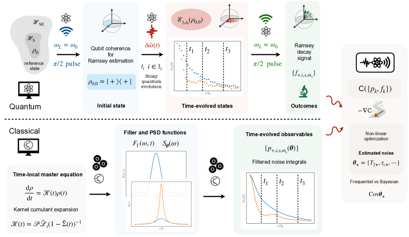
Figure 1: Scheme for L$\ell$QT protocol of a dynamical dephasing map: In the case of pure dephasing, the L$\ell$QT scheme reduces to a problem of Ramsey estimation. In the QIP, the qubit is initialized in a single state in the equator of Bloch’s sphere $\rho_{0,0}=\outerproduct{+}{+}$ by a resonant driving inducing a $\pi/2$ pulse on a reference state $\rho_{0}=\outerproduct{0}{0}$. The qubit then evolves for different times $t_{i}:i\in\mathbb{I}_{t}$, after which it is subjected to another resonant $\pi/2$ pulse, which effectively rotates to the Pauli measurement basis $x$. As a consequence of the dephasing noise, the $m_{x}\in\{0,1\}$ outcomes are collected as relative frequencies $\{f_{+,i,m_{x}}\}$ which will decay in time. In the lower half, we show the classical part of the estimation, which starts by solving the time-local master equation for a particular parametrized power spectral density $S_{\bm{\theta}}(\omega)$ and filter function. This leads to the theoretically predicted probabilities $\{p_{+,i,m_{x}}(\bm{\theta})\}$. These probabilities and the relative frequencies are fed into a log-likelihood cost function, which must be minimized in order to obtain the estimate. By calculating the covariance matrix, we can estimate the precision, and search for the optimal measurement times, which will depend on how many noise parameters we aim at estimating, and changes with their specific values. In a Bayesian approach, rather than minimizing a cost function built from the statistical likelihood, one updates the knowledge about the noise parameters sequentially by selecting the evolution times that are expected to provide most information at each Bayesian step.

Let us formulate the L$\ell$QT for the time-local master equation (8) for the dephasing of a single qubit, including temporal correlations. As discussed in Appendix A, either in a semi-classical or quantum-mechanical model of pure dephasing, the qubit dynamics can be described by a time-local master equation (8) with a simple Hamiltonian $H(t)=\textstyle\frac{1}{2}\omega_{0}\sigma_{z}$ and a single jump operator $L(t)=\sigma_{z}$, both of which are time independent

$$\frac{{\rm d}\rho}{{\rm d}t}=-\frac{\mathord{\rm i}}{2}\big{[}\omega_{0}\sigma_{z},\rho\big{]}+\gamma(t)\big{(}\sigma_{z}\rho\sigma_{z}-\rho\big{)}.$$ (12)

On the contrary, the decay rate is time-dependent and contains memory information about the noise fluctuations

$$\gamma(t)=\frac{1}{4}\int_{0}^{t}\!\!{\rm d}t^{\prime}\big{(}C(t,t^{\prime})+C(t^{\prime},t)\big{)}.$$ (13)

In a semi-classical model, $C(t,t^{\prime})=\mathbb{E}[\delta\tilde{\omega}(t)\delta\tilde{\omega}(t^{\prime})]$ is the auto-correlation function of a stochastic process $\delta\tilde{\omega}(t)$ representing frequency fluctuations. This master equation is the result of averaging over the stochastic process $\rho(t)=\mathbb{E}[\tilde{\rho}(t)]$, and is valid for a random process in a second-order cumulant expansion know as the fast-fluctuation expansion or, alternatively, for a Gaussian random process with arbitrary correlation times $\tau_{\rm c}$, as discussed in App. A. Alternatively, for a fully quantum-mechanical dephasing model, $C(t,t^{\prime})=\textstyle\frac{1}{2}{\rm Tr}_{B}\{B_{I}(t)B_{I}(t^{\prime})\rho^{\rm ss}_{\rm B}\}$ is the auto-correlation function on the stationary state of the environment/bath $\rho^{\rm ss}_{\rm B}$, which induces fluctuations in the qubit frequency via the bath operators $B_{I}(t)$. In this case, the time-local master equation is the result of tracing over the bath degrees of freedom $\rho(t)={\rm Tr}_{B}\{\rho_{\rm SB}(t)\}$, and is valid in a second-order cumulant expansion also discussed in App. A. Assuming wide-sense stationarity, i.e., the mean of the stochastic process is constant and the auto-correlation function only depends on $t^{\prime}-t$, we can introduce the power spectral density (PSD) of the noise

$$C(t-t^{\prime})=\int_{-\infty}^{\infty}\!\!\frac{{\rm d}\omega}{2\pi}\,S(\omega)\,\mathord{\rm e}^{\mathord{\rm i}\omega(t-t^{\prime})}.$$ (14)

Therefore, the time-dependent rate becomes

$$\gamma(t)=\frac{1}{2}\int_{-\infty}^{\infty}\!\!\!{{\rm d}\omega}\,S(\omega)\,f_{\gamma}(\omega,t),$$ (15)

where we have introduced the following modulation function

$$f_{\gamma}(\omega,t)=\frac{t}{2\pi}{\rm{sinc}}\,(\omega t).$$ (16)

It will be useful to define the symmetrized auto-correlation function and the symmetrized PSD as $\bar{C}(t,t^{\prime})=\frac{1}{2}(C(t,t^{\prime})+C(t^{\prime},t))$ and $\bar{S}(\omega)=\frac{1}{2}(S(\omega)+S(-\omega))$, since for dephasing noise only the symmetric part of the auto-correlation function and the symmetric part of the PSD influence the time evolution, as discussed in App. A.

In light of the L$\ell$QT estimation problem of Eq. (11), we do not need to consider arbitrary time-dependent functions for the Hamiltonian and dissipation matrix, but can actually find an effective parametrization that reduces drastically the search space. Considering Eq. (15), the dephasing rate will depend on a certain number $n$ of real-valued noise parameters $\bm{\theta}_{\!\star}\in\Theta=\mathbb{R}^{n}$ via the PSD $S_{\bm{\theta}_{\!\star}}\!(\omega)$, where we have made explicit its parametrization. Since the Hamiltonian of the qubit is very simple, and only depends on the transition frequency $\omega_{0}$ that is known with a high precision using spectroscopic methods, it need not be included in the learning. Technically, this means that we can assume that the driving used to initialize and measure the qubit is resonant with the transition (see Fig. 1), and work in the rotating frame of App. A. Likewise, we have only one possible jump operator $L=\sigma_{z}$, such that the learning can focus directly on the estimation $\bm{\hat{\theta}}$ of the actual noise parameters $\bm{{\theta}}_{\star}$, which translate into the estimation of the dephasing rate $\hat{\gamma}(t)$ via Eq. (15). Therefore, L$\ell$QT becomes a non-linear minimization problem for the cost function (9). Before giving more details on this problem, we discuss relevant properties of the dephasing quantum dynamical map.

For a white-noise noise model with a vanishing correlation time $\tau_{\rm c}=0$, one has a flat PSD $S(\omega)=c$ and a constant dephasing rate $\gamma(t)=c/2$. This leads to an exponential decay of the coherences $p_{+,i,x}(m_{x})=\textstyle\frac{1}{2}\big{(}1+(-1)^{m_{x}}\mathord{\rm e}^{-t_{i}/T_{2}}\big{)}$, where $m_{x}\in\{0,1\}$ correspond to the projective measurements on $\ket{+},\ket{-}$, respectively, and we have introduced a decoherence time $T_{2}=2/c$. If the real system is affected by white dephasing noise, there is thus a single noise parameter to learn $\theta_{\star}=c_{\star}$ or, alternatively, the real decoherence time $\theta_{\star}=T_{2\star}$. We note that this procedure is in complete agreement with the LQT based on the corresponding Lindblad master equation (2). On the other hand, for a time-correlated dephasing noise with a structured PSD, the coherence decay will generally differ from the above exponential law, with the exception of the long-time regime $t_{i}\gg\tau_{\rm c}$, where $p_{+,i,x}(m_{x})\approx\textstyle\frac{1}{2}\big{(}1+(-1)^{m_{x}}\mathord{\rm e}^{-t_{i}/T_{2}}\big{)}$ and one finds an effective decoherence time controlled by the static part of the PSD $T_{2}=2/S(0)$. As $t_{i}$ increases towards $\tau_{\rm c}$, the decay will no longer be a time-homogeneous exponential, which can actually be a consequence of (but not a prerequisite for) a non-Markovian quantum evolution. In this more general situation, we will have more noise parameters $\bm{\theta}_{\star}$ to learn.

Let us now connect to the formalism of filter functions [98, 99, 40, 41, 100, 43, 44, 101], which appears naturally when considering the time evolution of the coherences at any instant of time. This follows from the exact solution of the time-local master equation in the rotating frame, which reads

$$p^{\rm TL}_{+,i,x}(m_{x})=\frac{1}{2}\left(1+(-1)^{m_{x}}\mathord{\rm e}^{-\Gamma(t_{i})}\right)=:p_{i}^{\rm TL}(m_{x}),$$ (17)

where we have introduced the time integral of the decay rates

$$\Gamma(t)=2\int_{0}^{t}\!{\rm d}t^{\prime}\gamma(t^{\prime}),$$ (18)

and simplified the notation by omitting the initial state and the measurement basis, as they will be unique for the estimation of the dephasing map. Using the Fourier transform in Eq. (14), this integral can be rewritten in terms of the noise PSD as

$$\Gamma(t)=\!\int_{-\infty}^{\infty}\!\!\!\!{\rm d}\omega\,S(\omega)F_{\Gamma}(\omega,t),\hskip 4.30554ptF_{\Gamma}(\omega,t)=\!\int_{0}^{t}\!\!{\rm d}t^{\prime}\!f_{\gamma}(\omega,t^{\prime}),$$ (19)

where we have introduced a filter function that reads

$$F_{\Gamma}(\omega,t)=\frac{t}{2}\eta_{\frac{2}{t}}(\omega).$$ (20)

Note that, by making use of the nascent Dirac delta

$$\eta_{\epsilon}(x)=\frac{\epsilon}{\pi x^{2}}\sin^{2}\!\!\left(\,\frac{x}{\epsilon}\,\right),$$ (21)

where $\eta_{\epsilon}\!(x)\to\delta(x)$ as $\epsilon\to 0^{+}\!\!$, and $\int_{-\infty}^{\infty}\!{\rm d}x\,\eta_{\epsilon}\!(x)\!=1$, one sees that in the long-time limit $\epsilon=2/t\to 0^{+}$, $\tilde{f}_{\Gamma}(\omega,t)\approx\frac{t}{2}\delta(\omega)$ becomes a Dirac delta distribution, such that $\Gamma(t)\approx tS(0)/2$. This agrees with the above coarse-grained prediction for a decoherence time $T_{2}=2/S(0)$. Therefore, physically, the conditions for the long-time limit to be accurate is that $t\gg\tau_{\rm c}$.

In this article, we are not interested in this Markovian limit, as we aim at estimating the time-local master equation that depends on the full decay rate $\gamma(t)$, including situations in which non-Markovianity becomes manifest. To quantify this, we note that the dephasing quantum dynamical map

$$\mathcal{E}_{t,0}^{\rm TL}(\rho_{0})=(1-p(t))\rho_{0}+p(t)\sigma_{z}\,\rho_{0}\,\sigma_{z},$$ (22)

is non-Markovian when, at some intermediate time, there is no CPTP map $\mathcal{E}^{\rm TL}_{t,t^{\prime}}$ such that $\mathcal{E}_{t,0}^{\rm TL}=\mathcal{E}^{\rm TL}_{t,t^{\prime}}\circ\mathcal{E}^{\rm TL}_{t^{\prime},0}$ (7). In the above expression (22), we have introduced the following time-dependent probability for the occurrence of phase-flip errors

$$p(t)=\textstyle\frac{1}{2}\big{(}1-\mathord{\rm e}^{-\Gamma(t)}\big{)}.$$ (23)

Following [97], the degree of non-Markovianity of the quantum evolution can be obtained by integrating over all times for which the rate of the time-local master equation is negative

$$\mathcal{N}_{\rm CP}=\int{\rm d}t\big{(}|{\gamma}(t)|-{\gamma}(t)\big{)}.$$ (24)

An alternatively measure of non-Markovianity is based on the trace distance of two arbitrary initial states [102, 52], which will decrease with time when there is a flow of information from the system into the noisy environment. When this information flows back, the trace distance increases, and the qubit can recohere for a finite lapse of time, such that one gets a non-Markovian quantum evolution. The instantaneous variation of trace distance is given by $\sigma(t)=\frac{\differential}{\differential{t}}D(\mathcal{E}_{t,0}^{\rm TL}(\rho_{0}),\mathcal{E}_{t,0}^{\rm TL}(\rho_{0}^{\prime}))$, with $D$ being the trace distance [1], and a positive $\sigma(t)$ is thus a measure of non-Markovianity, which can be expressed in terms of the time intervals in which the phase-flip error probability decreases infinitesimally with time

$$\mathcal{N}_{\mathrm{TD}}=\max_{\rho_{0},\rho_{0}^{\prime}}\int_{\sigma(t)>0}\differential{t}\sigma(t)=-\int_{\gamma(t)<0}\differential{t}\dot{p}(t).$$ (25)

Here, we have rewritten this measure in terms of the error probability of the phase-flip channel (23), which changes infinitesimally with $\dot{p}(t)=\gamma(t)\mathord{\rm e}^{-\Gamma(t)}$. Hence, the non-Markovianity condition translates into a dynamical situation in which phase-flip errors do not increase monotonically during the whole evolution. When the dephasing rate attains negative values, the phase-flip error probability can decrease, such that the qubit momentarily recoheres (see the orange lines in Fig. 1). In this simple case of pure dephasing noise, we see that both measures of non-Markovianity in Eqs. (24) and  (25) depend on the rate $\gamma(t)$ attaining negative values, and both are equal to 0 if $\gamma(t)$ is always positive.

Once these additional properties of the dephasing quantum dynamical map have been discussed, we can move back to the estimation L$\ell$QT protocol (11), and how it can be simplified even further. As noted above, in contrast to the informationally-complete set of initial states an measurements that must be considered for the general cost function of L$\ell$QT (9), we can work with a smaller number of configurations by noting that all information of the dephasing map can be extracted by preparing a single initial state $\rho_{0}=\outerproduct{+}{+}$, and measuring in a single basis $M_{x,\pm}$ (see Fig. 1). As advanced in the introduction, we would like to know how many snapshots $|\mathbb{I}_{t}|$ are required, at which the system is measured after evolving for $\{t_{i}:\,i\in\mathbb{I}_{t}\}$ and, moreover, which are the optimal times of those snapshots in terms of the specific details of the noise. We take here two different routes. On the one hand, we can follow a frequentist approach similarly to the one in Markovian Lindblad quantum tomography [87, 89, 90], but now taking into account the time-dependence of the decay rates, which will require an a priori selection of the evolution times at which the system is probed. Alternatively, we also consider a Bayesian approach that exploits a physically-motivated prior knowledge about the noise parameters, which can be represented by a certain probability distribution. After performing measurements on the system at certain instants of time, we update this probability distribution with the new acquired information, a process that is repeated until reaching a target accuracy for the parameter estimation. The Bayesian approach has the advantage of choosing, at each step, the most convenient subsequent time at which to measure by maximizing the information one would gain. In principle, this can lead to a reduction in the number of measurements required to reach a certain accuracy with respect to those required by the frequentist approach. In practice, however, the non-Markovianity of the quantum evolution can modify this argument, as our probabilistic account of the model parameters can be affected by the actual time correlations of the underlying random process. We present below a detailed comparison of the two approaches, determining the regimes in which each of them is better than the other.

III.1 ​Frequentist approach to non-Markovian inference

In this section, we focus on the frequentist approach, which builds on the relative frequencies of observed outcomes. The L$\ell$QT cost function (9) can be rewritten as follows

$$\mathsf{C}^{\rm pd}_{\mathrm{TL}}(\bm{\theta})=-\sum_{i}N_{i}\,\sum_{m_{x}}\,\tilde{f}_{i}(m_{x}\,|\bm{\theta}_{\star})\log p^{\rm TL}_{i}(m_{x}|\bm{\theta}),$$ (26)

which is greatly simplified with respect to the general case in Eq. (5), as we only have a single initial state and a single measurement basis. Since we are monitoring the coherence of the qubit, this cost function corresponds to a Ramsey-type estimator, where $\tilde{f}_{i}(0\,|\bm{\theta}_{\star})=N_{i,0}/N_{i}$ $(\tilde{f}_{i}(1\,|\bm{\theta}_{\star})=N_{i,1}/N_{i})$ is the ratio of the number of outcomes observed $N_{i,0}$ ($N_{i,1}=N_{i}-N_{i,0}$) to the total of $N_{i}$ shots collected at the instant of time $t_{i}$, when measuring the system with the POVM element $M_{x,0}$ ($M_{x,1}$). Our notation remarks that these relative frequencies carry information about the real noise parameters $\bm{\theta}_{\!\star}$ we aim at estimating. In addition, the estimator depends on $p_{i}(m_{x}|\bm{\theta})$ (17)-(18), which stand for the probabilities obtained by solving the time-local dephasing master equation (12), where we make explicit the dependence on the parametrized noise.

The minimization (11) is simplified in this case, as one can dispense with the time-dependent constraints. As a consequence, the frequentist approach can be recast as a statistical problem of parameter point estimation [96], namely

$$\bm{\hat{\theta}}_{\rm F}=\texttt{argmin}_{\bm{\theta}}\{\mathsf{C}^{\rm pd}_{\mathrm{TL}}(\bm{\theta}):\,\bm{\theta}\in\Theta=\mathbb{R}^{n}\}.$$ (27)

Instead of the general L$\ell$QT learning over $d^{2}(d^{2}-1)$ parameters, which increase exponentially $d=2^{n_{q}}$ with the number of qubits $n_{q}$ and can arbitrarily change in time, our procedure revolves around the estimation of $n$ noise parameters, which are independent of the system size and the evolution times. On the other hand, the imprecision of our estimates will indeed depend on our choice of the evolution times, forcing us to go beyond the LQT single-time estimator [90], and actually measure at optimal times for which the estimation imprecision can be minimized. Let us note that the conditions to minimise this cost function are the same as those that minimize the Kullback-Leibler divergence [103, 104], which is the following relative entropy

$$\mathsf{D}_{\rm KL}(\bm{p}_{1}||\,\bm{p}_{2})=-\sum_{k}p_{1,k}\log\left(\frac{p_{2,k}}{p_{1,k}}\right),$$ (28)

between the experimental $p_{1,k}\in\{\tilde{f}_{i}(+\,|\bm{\theta}_{\star}),(1-\tilde{f}_{i}(+\,|\bm{\theta}_{\star}))\}$ and parametrized theoretical $p_{2,k}\in\{p^{\rm TL}_{i}(+\,|\bm{\theta}),p^{\rm TL}_{i}(-\,|\bm{\theta})\}$ probability distributions, provided one considers variations with respect to the estimation parameters $\bm{\theta}$.

The above estimator depends on the data set $\mathbb{D}$, and is thus also a stochastic variable, which will be characterized by its mean $\mathbb{E}[\bm{\hat{\theta}}_{\rm F}]$ and its moments, such as the covariance matrix

$$[\mathrm{Cov}(\bm{\hat{\theta}}_{\rm F})]_{n_{1},n_{2}}=\mathbb{E}\big{[}\big{(}\hat{\theta}_{n_{1}}-\mathbb{E}[\hat{\theta}_{n_{1}}]\big{)}\big{(}\hat{\theta}_{n_{2}}-\mathbb{E}[\hat{\theta}_{n_{2}}]\big{)}\big{]}.$$ (29)

We note that the expectation values are taken with respect to the probability distributions for the measurements (3) which, implicitly, also have the stochastic average over the random dephasing noise in the semi-classical model, or a partial trace over the environment/bath in the quantum-mechanical one. The nice property of the maximum-likelihood estimator is that it is asymptotically unbiased, such that $\bm{\mathsf{B}}_{\bm{\theta}_{\star}}\!\!(\bm{\theta}_{\rm F})=\mathbb{E}[\bm{\hat{\theta}}_{\rm F}]-\bm{\theta}_{\star}\to\bm{0}$ for a sufficiently-large $N_{\rm shot}\gg 1$. Moreover, its asymptotic covariance matrix saturates the Cramér-Rao bound [105] relating the estimation precision to the Fisher information matrix, which quantifies the amount of information in $\mathbb{D}$ about the unknown parameters. If we momentarily assume that the measurements occur at a single instant of time $t=t_{i}$ with outcomes that are independent and identically distributed, the covariance matrix becomes $\mathrm{Cov}(\bm{\hat{\theta}}_{\rm F})\approx(N_{i}{I}_{F,i}(\bm{\theta}_{\!\star}))^{-1}$, where

$$[{I}_{F,i}(\bm{\theta}_{\!\star})]_{n_{1},n_{2}}=\mathbb{E}\left[\left.\frac{\partial{\rm log}\big{(}p_{i}^{\rm TL}(m_{x}|\bm{\theta})\big{)}}{\partial{\theta_{n_{1}}}}\frac{\partial{\rm log}\big{(}p_{i}^{\rm TL}(m_{x}|\bm{\theta})\big{)}}{\!\partial\theta_{n_{2}}}\!\right|_{\bm{\theta}_{\star}}\right].$$ (30)

In this work, we deal with the more general case in which we measure at several times, therefore the random variables are not identically distributed, and the total number of shots need not be the same for different times. In this case, we must take a linear combination of the Fisher information matrices of each measurement time weighted by the proportion of measurements taken at each time  [106]. We thus obtain the asymptotic covariance matrix

$$\mathrm{Cov}(\bm{\hat{\theta}}_{\rm F})\approx\Sigma_{\bm{\hat{\theta}}}\equiv\left[N_{\rm shot}\sum_{i}\frac{N_{i}}{N_{\rm shot}}{I}_{F,i}(\bm{\theta}_{\!\star})\right]^{-1},$$ (31)

such that, the more the Ramsey estimator varies under changes of the noise parameters, the bigger the amplification of the noise parameter is and, thus, the smaller the imprecision one can achieve. As we can see, the imprecision of the estimate will scale with $1/\sqrt{N_{\rm shot}}$, such that the Ramsey estimator is asymptotically consistent in the $N_{\rm shot}\gg 1$ asymptotic limit [96]. The asymptotic statistics of the maximum-likelihood estimator is further explained in App. D.

We also note that, in this limit, the observed relative frequencies will be normally distributed, such that one can consider minimizing the weighted least-squares cost function

$$\mathsf{C}_{\mathrm{TL}}^{\rm pd}(\bm{\theta})\approx\sum_{i}\frac{\big{(}\tilde{f}_{i}(0\,|\bm{\theta}_{\star})-p_{i}^{\rm TL}(0|\bm{\theta})\big{)}^{2}}{\tilde{\sigma}^{2}_{f_{i}}},$$ (32)

where $\tilde{\sigma}^{2}_{f_{i}}$ is the variance of the measured samples. For large $N_{i}$ the expected variance of the measurements at time $t_{i}$ is

$$\sigma^{2}_{f_{i}}=\frac{p_{i}^{\rm TL}(0\,|\bm{\theta})\big{(}1-p_{i}^{\rm TL}(0\,|\bm{\theta})\big{)}}{N_{i}},$$ (33)

since we are sampling from a binomial distribution. This approximation allows us to use a simpler weighted least-squares algorithm, such as the trust-region reflective algorithm implemented in SciPy, where we can optionally set some bounds for the parameters to be estimated [107].

Once the properties of the Ramsey frequentist estimate $\bm{\hat{\theta}}_{\rm F}$ have been discussed, we can search for the optimal measurement times that would lead to a Ramsey estimator with the lowest possible imprecision for a given finite $N_{\rm shot}$. Depending on which parameter we are interested in, we may be interested in minimizing a particular component of the covariance matrix $[\Sigma_{\bm{\hat{\theta}}}]_{n_{1},n_{1}}$ (31) or, alternatively, minimize its determinant as a whole. In the asymptotic limit in which $\bm{\hat{\theta}}_{\rm F}$ follows a multivariate normal distribution, $\det\Sigma_{\bm{\hat{\theta}}}$ is proportional to the volume enclosed by the covariance elliptical region, so it is a good measure of the dispersion of the distribution, and a good way to quantify the accuracy of the estimation. Sometimes, we will also use $\det\Sigma_{\bm{\hat{\theta}}}^{1/2n}$ instead, which can be more easily compared to the individual standard deviations $[\Sigma_{\bm{\hat{\theta}}}]_{n_{1},n_{1}}^{1/2}$, as both quantities scale with $1/\sqrt{N_{\rm shot}}$. Minimizing $\det\Sigma_{\bm{\hat{\theta}}}$ has also the advantage that the optimal measurement times obtained are independent of the parameters we want to determine, assuming the different parametrizations have the same number of parameters and that a coordinate transformation exists between parametrizations. In this case, the determinants of the covariance matrices are related by $\det\Sigma_{\bm{\hat{\theta}}}=\det\Sigma(\bm{\hat{\theta}}^{\prime}_{\rm F})\det J^{2}$, with $J$ the Jacobian of the coordinate transformation between both parametrizations, which does not depend on time and therefore will have no influence in the minimization. Before presenting these results, we discuss an approach based on Bayesian inference [96].

III.2 ​Bayesian approach to non-Markovian inference

Rather than considering the relative frequencies as approximations of the underlying probability distribution with a certain fixed value of $\bm{\theta}_{\star}$, the idea of Bayesian inference is to quantify statistically our knowledge about the noise parameters, and how this knowledge gets updated as we collect more information via measurements. Hence, the noise parameters become continuous stochastic variables themselves $\bm{\theta}_{\star}\mapsto\bm{\tilde{\theta}}$ that take values $\bm{\theta}\in\Theta$ according to a prior pdf $\pi_{0}(\bm{\theta})$. This probability distribution quantifies our uncertainty about the noise parameters before making any measurement $\mathbb{D}_{0}=\emptyset$. At each $\ell>0$ Bayesian step, we measure the system enlarging the data set sequentially $\mathbb{D}_{\ell-1}\mapsto\mathbb{D}_{\ell}=\mathbb{D}_{\ell-1}\cup\delta\mathbb{D}_{\ell}$, where $\delta\mathbb{D}_{\ell}\subset\mathbb{D}=\{N_{i,+,x,m_{x}}\}$ contains a number of measurement outcomes $|\delta N_{\ell}|$ that is a fraction of the total $N_{\rm shot}$. These outcomes will be labelled as $\delta\mathbb{D}_{\ell}=\{N_{i_{\ell},+,x,m_{x_{\ell}}}\}$. The measurements in this data set are again binary Bernoulli trials, and can be described by a joint multinomial distribution $p_{\tilde{N}}(\delta\mathbb{D}_{\ell})$ defined in analogy to Eq. (4), but only extended to the configurations measured in the particular Bayesian step. The prior $(\ell-1)$-th probability distribution is then updated by using Bayes’ rule based on the parametrized probability distributions $p^{\rm TL}_{\ell}(\delta{\mathbb{D}}_{\ell}|\bm{\theta})$ being understood as probabilities conditioned on our statistical knowledge of the noise parameters

$$\pi_{\ell}(\bm{\theta}|\mathbb{D}_{\ell})=\frac{1}{p^{\rm TL}_{\ell-1}(\delta\mathbb{D}_{\ell})}p^{\rm TL}_{\ell}(\delta\mathbb{D}_{\ell}|\bm{\theta})\pi_{\ell-1}(\bm{\theta}).$$ (34)

Here, $p^{\rm TL}_{\ell-1}(\delta\mathbb{D}_{\ell})=\int_{\Theta}\differential^{n}{\theta}p^{\rm TL}_{\ell}(\delta\mathbb{D}_{\ell}|\bm{\theta})\pi_{\ell-1}(\bm{\theta})$ is a normalization constant required to interpret $\pi_{\ell}(\bm{\theta}|\mathbb{D}_{\ell})\mapsto\pi_{\ell}(\bm{\theta})$ as a probability distribution describing our updated knowledge about the noise, which will be used as the subsequent prior.

One of the main differences with respect to the frequentist approach is that we have, at each step, a probability distribution from which one can obtain a Bayesian estimate

$$\bm{\hat{\theta}}_{{\rm B}}=\mathbb{E}_{\bm{\theta}}[\bm{\theta}]=\int_{\Theta}\!{\rm d}^{n}\theta\,\pi_{\ell}(\bm{\theta})\bm{\theta}.$$ (35)

We note that this Bayesian estimator $\hat{\bm{\theta}}_{\rm B}$ minimizes the Bayesian risk associated to a squared error loss function over all possible estimators $\hat{\tau}$, $\bm{\hat{\theta}}_{{\rm B}}=\texttt{argmin}\{\mathsf{R}_{\rm TL}(\hat{\tau})\}$ [96] with

$$\mathsf{R}_{\rm TL}(\hat{\tau})=\!\sum_{i_{\ell},m_{x_{\ell}}\in\delta\mathbb{D}_{\ell}}\int_{\Theta}\!{\rm d}^{n}\theta\,\pi_{\ell}(\bm{\theta})p^{\rm TL}_{\ell}\big{(}\delta\mathbb{D}_{\ell}|\bm{\theta}\big{)}(\hat{\tau}-\bm{\theta})^{2}.$$ (36)

In addition to the expectation value (35), since we have the updated probability distributions, we can quantify how our uncertainty about the noise parameters changes via the associated covariance matrix $[\mathrm{Cov}(\bm{\hat{\theta}}_{{\rm B}})]_{n_{1},n_{2}}$ or any other statistics, regardless of the size of the Bayesian data set $\mathbb{D}_{\ell}$. This differs from our previous arguments for covariance of the maximum likelihood estimate $\bm{\hat{\theta}}_{\rm F}$ (31), which require working in the asymptotic regime $N_{\rm shot}\gg 1$. In experimental situations in which this regime cannot be reached, we note that one could use Monte Carlo sampling techniques to estimate precision of $\bm{\hat{\theta}}_{\rm F}$ [108, 109, 77], although these deal with the estimator based on the full likelihood function in Eq. (4).

Another crucial difference of the Bayesian approach is that, instead of choosing a predefined set of evolution times $\{t_{i}:\,\in\mathbb{I}_{t}\}\subset T$, either distributed uniformly, randomly, or at precise instants to minimise the covariance, we can find the optimal time at which we should measure to maximize the information gain at each Bayesian step. For each update, we thus solve for

$$t_{\ell}=\texttt{argmax}_{t}\big{\{}\mathbb{E}\left[\mathsf{D}_{\mathrm{KL}}\big{(}\pi_{\ell}(\bm{\theta}|\mathbb{D}_{\ell})\,\big{|}\!\big{|}\,\pi_{\ell}(\bm{\theta})\big{)}\right]\big{\}},$$ (37)

where $\pi_{\ell}(\bm{\theta}|\mathbb{D}_{\ell})$ is the posterior probability (34) corresponding to the measurement results one would obtain by measuring at a time $t$ and enlarging the data set as $\mathbb{D}_{\ell^{\prime}}=\mathbb{D}_{\ell}\cup\delta\mathbb{D}_{\ell^{\prime}}$. In the expression above, we are making use of the Kullback-Leibler divergence (28) between the posterior and the prior, searching for a time that maximizes the relative entropy between the prior and any of the possible posteriors, such that one gains the maximum amount of information at each Bayesian step. Therefore, not only the data set is enlarged sequentially $\mathbb{D}_{\ell}\supset\mathbb{D}_{\ell-1}$, but also the specific times are chosen adaptively. In light of the fixed set of measurement times in the frequentist approach $\{t_{i}:\,i\in\mathbb{I}_{t}\}$, we note that the total set of updated times after $N_{\rm B}$ Bayesian steps $\{t_{\ell},\ell\in\{0,\cdots,N_{\rm B}\}\}$ can be very different, and that is the reason why we use a different notation. Computing Eq. (37) can be quite time-consuming, especially when dealing with a large number of parameters. In practice, long computation times may lead to a reduction in the frequency of experimental shots, which is undesirable. To avoid this, we can take tenths or hundreds of shots at each step before computing again the optimal measurement time. This will not change the results significantly, since a Bayesian update of a single shot does not change the prior much and the optimal measurement time of next step remains very similar to the previous one.

We note that the Bayesian approach is ultimately related to the maximum-likelihood estimation in the asymptotic limit $N_{\rm shot}\gg 1$. When the variance of the prior is small, the maxima of the Kullback-Leibler divergence (28) between prior and posterior are localized at the optimal times obtained by minimizing the asymptotic covariance matrix of the maximum likelihood-estimation (31). Additionally, if we make a single Bayesian update in which we take a very big number of shots at several times, the likelihood function relating the posterior and the prior will be a multinomial pdf (4). Given the big number of shots taken in this single step, the posterior distribution will be mainly shaped by the likelihood function, which contains most of the information about the parameters. The position of the maximum of this pdf will be located at the most likely value of the parameters, and therefore it is in agreement with the maximum-likelihood estimator that takes measurements at those times. The Bayesian approach has the advantage that, at each step, we measure at the most convenient time that maximizes the expected information gain, and this can lead to an overall reduction of the number of measurements needed. Also, as noted above, the final estimate relies on a probability distribution, so that we can immediately derive confidence intervals without requiring any asymptotic limit. For the Bayesian protocol design, we have used the Python package Qinfer [110], which numerically implements the operations needed by using a sequential Monte Carlo algorithm for the updates.

III.3 ​ Comparative performance analysis

Let us now study some dephasing dynamics in which we can apply the two approaches we have just introduced, and make a comparative study of their performance when learning parametrized dephasing maps with time-correlated noise.

III.3.1 Markovian semi-classical dephasing

We now apply both estimation techniques for the L$\ell$QT of a dephasing quantum dynamical map that goes beyond the Markovian Lindblad assumptions. In particular, we consider a time-correlated frequency noise $\delta\tilde{\omega}(t)$ that is described by an Ornstein-Uhlenbeck (OU) random process [111, 112]. This process has an underlying multi-variate Gaussian joint pdf, and incorporates a correlation time $\tau_{\rm c}>0$ above which the correlations between consecutive values of the process become very small. In fact, beyond the relaxation window $t,t^{\prime}>\tau_{\rm c}$, the correlations show an exponential decay

$$C(t-t^{\prime})=\frac{c\tau_{\rm c}}{2}\mathord{\rm e}^{-\frac{|t-t^{\prime}|}{\tau_{\rm c}}},$$ (38)

where $c>0$ is a so-called diffusion constant. Since this correlations only depend on the time differences, the process is wide-sense stationary. Moreover, on the basis of its Gaussian joint pdf, it can be shown that the process is indeed strictly stationary. Being Gaussian, all the information is thus contained in its two-point functions or, alternative, in its PSD (59)

$$S(\omega)=\frac{c\tau_{\rm c}^{2}}{1+(\omega\tau_{\rm c})^{2}},$$ (39)

which has a Lorentzian shape. This Gaussian process then leads to an exact time-local master equation for the dephasing of the qubit (12) with a time-dependent decay rate

$$\gamma(t)=\textstyle\frac{1}{4}S(0)\left(1-\mathord{\rm e}^{-\frac{t}{\tau_{\rm c}}}\right).$$ (40)

In the long-time limit $t\gg\tau_{\rm c}$, one recovers a constant decay rate $\gamma(t)\approx S(0)/4=c\tau_{\rm c}^{2}/4$, which connects to our previous discussion of the effective exponential decay of the Ramsey signal $p^{\rm TL}_{i}(m_{x})\approx\big{(}1+(-1)^{m_{x}}\mathord{\rm e}^{-t_{i}/T_{2}}\big{)}/2$ and the decoherence time $T_{2}=2/c\tau_{\rm c}^{2}$. On the other hand, for shorter time scales, we see the effects of the noise memory through a time-inhomogeneous evolution of the coherences that goes beyond a Lindbladian description. It is interesting to remark that, in spite of not being a Lindbladian evolution, the time-dependent decay rate is always positive, such that the two measures of non-Markovianity in Eqs. (24)-(25) vanish exactly. The pure dephasing quantum dynamical map of a qubit subjected to OU frequency noise is thus Markovian albeit not Lindbladian.

From the perspective of L$\ell$QT, we have two parameters to learn $\bm{\theta}=(c,\tau_{\rm c})\in\Theta=\mathbb{R}_{+}^{2}$, which fully parametrize the PSD, the decay rate or, alternatively, the Ramsey attenuation factor

$$\Gamma(t)=\textstyle\frac{1}{2}S(0)\left(t-\tau_{\rm c}\big{(}1-\mathord{\rm e}^{-\frac{t}{\tau_{\rm c}}}\big{)}\right).$$ (41)

Frequentist Ramsey estimators.

We can now evaluate the L$\ell$QT cost function $\mathsf{C}^{\rm pd}_{\mathrm{TL}}(\bm{\theta})$ in Eq. (26) by substituting the attenuation factor (41) in the likelihood function $p^{\rm TL}_{i}(m_{x}|\bm{\theta})=\big{(}1+(-1)^{m_{x}}\mathord{\rm e}^{-\Gamma(t_{i})}\big{)}/2$ after a certain set of evolution times $\{t_{i},i\in\mathbb{I}_{t}\}$, and the relative frequencies for the measurement outcomes $\tilde{f}_{i}(m_{x}\,|\bm{\theta}_{\star})$. For a Lindbladian dynamics, a single measuring time $t_{1}$ would suffice for the estimation [90], which can actually be solved for analytically in the present pure dephasing context, as discussed in App. B. For the OU dephasing, this is no longer the case, and we actually need at least two times $t_{1},t_{2}$. In order to assess the performance of the frequentist minimization problem (27) under shot noise, we numerically generate the relative frequencies $\tilde{f}_{1}(m_{x}\,|\bm{\theta}_{\star}),\tilde{f}_{2}(m_{x}\,|\bm{\theta}_{\star})$ at two instants of time by sampling the probability distribution with the actual OU parameters $\bm{\theta}_{\star}=(c_{\star},\tau_{\rm c{\star}})$ a number of times $N_{\rm shot}=N_{1}+N_{2}$. In the following, rather than learning $(c_{\star},\tau_{\rm c\star})$, we will focus on two noise parameters with units of time $(T_{2\star},\tau_{\rm c\star})$, where we recall that $T_{2\star}=2/c^{\phantom{2}}_{\star}\tau_{{\rm c}\star}^{2}$ is an effective decoherence time in the long-time limit. In Fig. 2, we present a contour plot of this two-time cost function $\mathsf{C}^{\rm pd}_{\mathrm{TL}}(\bm{\theta})$, which is actually convex and allows for a neat visualization of its global minimum. We also depict with a red cross the result of a gradient-descent minimization, where one can see that the estimates $\bm{\hat{\theta}}_{\rm F}=(\hat{T}_{2},\hat{\tau}_{\rm c})$ are close to the real noise parameters. The imprecision of the estimate is a result of the shot noise, which we now quantify.

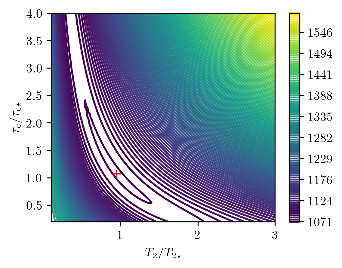
Figure 2: Gradient descent for OU dephasing L$\ell$QT: Contour plot of the Ramsey cost function $\mathsf{C}^{\rm pd}_{\mathrm{TL}}(\bm{\theta})$ of Eq. (26) as a function of the noise parameters $(T_{2},\tau_{\rm c})$, where we recall that $T_{2}=2/c\tau_{\rm c}^{2}$ plays the role of an effective decoherence time in the long-time limit. We choose two evolution times and, for illustration purposes, fix them at $t_{1}=\tau_{\rm c\star}$, $t_{2}=2\tau_{\rm c\star}$, fixing the OU diffusion constant such that $T_{2\star}/\tau_{\rm c\star}=1$. We distribute $N_{\rm shot}=2\times 10^{3}$ shots equally per time step. The gradient descent of this convex problem converges towards the global minimum, and is marked with a red cross that lies close to the real noise parameters $\bm{\theta}\mapsto\bm{\theta}_{\star}$.

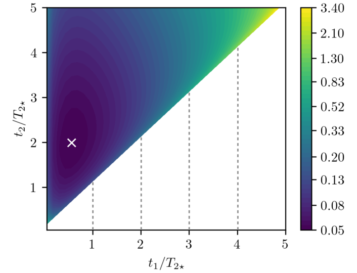
Figure 3: Asymptotic covariance matrix for OU dephasing: We represent $\det(\Sigma_{\bm{\hat{\theta}}}(t_{1},t_{2}))^{1/2}$ as a function of the $t_{1}$ and $t_{2}$ measurement times selected. For $t_{1}=t_{2}$ the determinant diverges, since it is not possible to determine the parameters by just measuring at a single time. The true parameters are $\tau_{\rm c\star}=T_{2\star}/2$ and the number of shots is $N_{1}=N_{2}=5\cdot 10^{3}$. The optimal times that minimize the determinant are indicated with a white cross, $t_{1}\approx 0.56T_{2\star}$, $t_{2}\approx 1.99T_{2\star}$. The determinant increases rapidly when moving away from this minimum. Note the color bar scale is logarithmic. The plot is symmetric with respect to the line $t_{1}=t_{2}$, therefore we just represent the part $t_{2}>t_{1}$.

In order to find the optimal evolution times $t_{1},t_{2}$ that maximize the precision of our estimates, we can minimize the covariance in Eq. (31) which, in turn, requires maximizing the Fisher information matrix (30). By Taylor expanding the cost function, we can actually find a linear relation between the estimate difference $\delta{\bm{\hat{\theta}}}=\bm{\hat{\theta}}_{{\rm F}}-\bm{\theta}_{\star}$, and the differences between the parametrized probabilities and the relative frequencies $\delta\tilde{f}_{i}=p_{i}^{\rm TL}(m_{x}|\bm{\hat{\theta}})-\tilde{f}_{i}(m_{x}\,|\bm{\theta}_{\star})$, namely

$$\begin{pmatrix}\delta\hat{T}_{2}\\ \delta\hat{\tau}_{\rm c}\end{pmatrix}\!=\!\frac{1}{\mathcal{N}}\!\!\begin{pmatrix}-\frac{\Gamma^{\prime}_{\tau_{\rm c}}\!(t_{2})(\mathord{\rm e}^{2\Gamma(t_{1})}-1)}{\sinh\Gamma(t_{1})}&\frac{\Gamma^{\prime}_{\tau_{\rm c}}\!(t_{1})(\mathord{\rm e}^{2\Gamma(t_{2})}-1)}{\sinh\Gamma(t_{2})}\\ \frac{\Gamma^{\prime}_{T_{2}}\!\!(t_{2})(\mathord{\rm e}^{2\Gamma(t_{1})}-1)}{\sinh\Gamma(t_{1})}&-\frac{\Gamma^{\prime}_{T_{2}}\!\!(t_{1})(\mathord{\rm e}^{2\Gamma(t_{2})}-1)}{\sinh\Gamma(t_{2})}\end{pmatrix}\!\!\!\begin{pmatrix}\delta\tilde{f}_{1}\\ \delta\tilde{f}_{2}\end{pmatrix}\!,$$ (42)

where $\mathcal{N}=\Gamma^{\prime}_{T_{2}}\!(t_{1})\Gamma^{\prime}_{\tau_{\rm c}}\!(t_{2})-\Gamma^{\prime}_{\tau_{\rm c}}\!(t_{1})\Gamma^{\prime}_{T_{2}}\!(t_{2})$, and we have introduced a shorthand notation for the partial derivatives $\Gamma^{\prime}_{\tau}\!(t_{i})=\partial\Gamma(t_{i})/\partial\tau_{\rm c}$, $\Gamma^{\prime}_{T_{2}}\!(t_{i})=\partial\Gamma(t_{i})/\partial T_{2}$. The first thing one notices is that, fixing $t_{2}=t_{1}$, the factor $\mathcal{N}=0$, and the difference between the estimation and the true value of the parameters diverges, signaling the fact that one cannot learn two noise parameters using a Ramsey estimator with a single instant of time. The second result one finds is that, in the asymptotic limit $N_{i}\gg 1$, the estimate differences will follow a bi-variate normal distribution. This follows from the fact that Eq. (42) is a linear combination of the differences between the finite frequencies and the binomial probabilities, which are known to follow a normal distribution $N(\bm{0},{\rm diag}\big{(}\sigma^{2}_{f_{1}},\sigma^{2}_{f_{2}})\big{)}$ with binomial variances $\sigma^{2}_{f_{i}}$ defined in Eq. (33). Therefore, the frequentist estimates will also be normally distributed $\delta{\bm{\hat{\theta}}}\sim N(\bm{0},\Sigma_{\bm{\hat{\theta}}}\big{)}$ according to

$$\Sigma_{\bm{\hat{\theta}}}(t_{1},t_{2})=M_{\bm{\hat{\theta}}}(t_{1},t_{2})\begin{pmatrix}\sigma^{2}_{f_{1}}&0\\ 0&\sigma^{2}_{f_{2}}\end{pmatrix}M_{\bm{\hat{\theta}}}^{\rm T}(t_{1},t_{2}),$$ (43)

where $M_{\bm{\hat{\theta}}}(t_{1},t_{2})$ is the matrix in Eq. (42). A more detailed derivation of the relationship between shot noise and the uncertainty in estimation, as well as the asymptotic covariance matrix, is provided in App. D. From this perspective, the aforementioned divergence for $t_{1}=t_{2}$ is a consequence of the singular nature of this matrix, which cannot be thus inverted.

A measure of the imprecision of the estimation is then obtained from $\det(\Sigma_{\bm{\hat{\theta}}}(t_{1},t_{2}))=(\det M_{\bm{\hat{\theta}}})^{2}\sigma^{2}_{f_{1}}\sigma^{2}_{f_{2}}\propto 1/N_{1}N_{2}=1/N_{1}(N_{\rm shot}-N_{1})$ which, in this bi-variate case, can be related to the area enclosed by a covariance ellipse. We thus clearly see that the maximum precision will be obtained when $N_{1}=N_{2}=N_{\rm shot}/2$. Turning to the optimal measurement times, we can now numerically minimize the determinant of the asymptotic covariance matrix

$$\{t_{i,{\rm opt}}\}=\texttt{argmin}\left\{\det\Sigma_{\bm{\hat{\theta}}}\big{(}\{t_{i}\}\big{)}\right\},$$ (44)

finding the two optimal values at which the signal shows the highest sensitivity to changes in the OU noise (see Fig. 3). The optimal times obtained in this way are depicted in Fig. 4 as a function of the noise correlation time. In the limit where this correlation time is much smaller than the effective decoherence time $\tau_{\rm c\star}\ll T_{2\star}$, the signal only carries important information about the noise for times that are much larger than the correlation time. Hence, we are in the long-time limit where the decay rate is constant $\gamma(t)\approx 1/2T_{2}$ and one expects to find agreement with a purely Lindbladian dephasing noise. As discussed in App. B, the LQT for pure dephasing requires a single measuring time, and can be analytically found by minimizing the standard deviation of the estimated noise parameter (65). This solution yields an optimal time $t_{\rm opt}=0.797T_{2\star}$, which is actually very close to the intercept of the curve of $t_{2,{\rm opt}}$ shown in Fig. 4. In this long-time regime, we find $t_{1,{\rm opt}}\approx 0$ indicating that measurements at time $t_{2,\rm opt}$ will be mainly used to determine parameter $T_{2}$, while those at $t_{1,{\rm opt}}\approx 0$ contribute to determine the much smaller $\tau_{\rm c}$.

In the more general case in which the time correlation of the OU noise yields important memory effects, the measurement times have to be adapted to specific optimal values, which are in general larger than the purely Lindbladian limit as shown in Fig. 4. Since these optimal times depend on the parameters we aim at learning, it is not straightforward to devise a practical strategy to minimise the imprecision of the frequentist estimates. In the pure Lindbladian case, one may foresee that the experimentalist will have an accurate prior knowledge of the $T_{2}$ time, such that the measurements can all be implemented close to the predicted optimal time. On the other hand, for the OU noise, one has the additional noise correlation time $\tau_{\rm c}$, which is related to deviations from the time-homogeneous exponential decay of the coherences and is not typically characterised experimentally. The frequentist procedure to operate at the optimal regime of estimation would then need to distribute the total $N_{\rm shot}$ in smaller groups that are applied in sequence, each time shifting the measurement times to try to get to the optimal point. One can foresee that this procedure will not be optimal, as one will loose many measurements along the way and, moreover, not scalable to other situations in which one aims at learning more noise parameters also optimally.

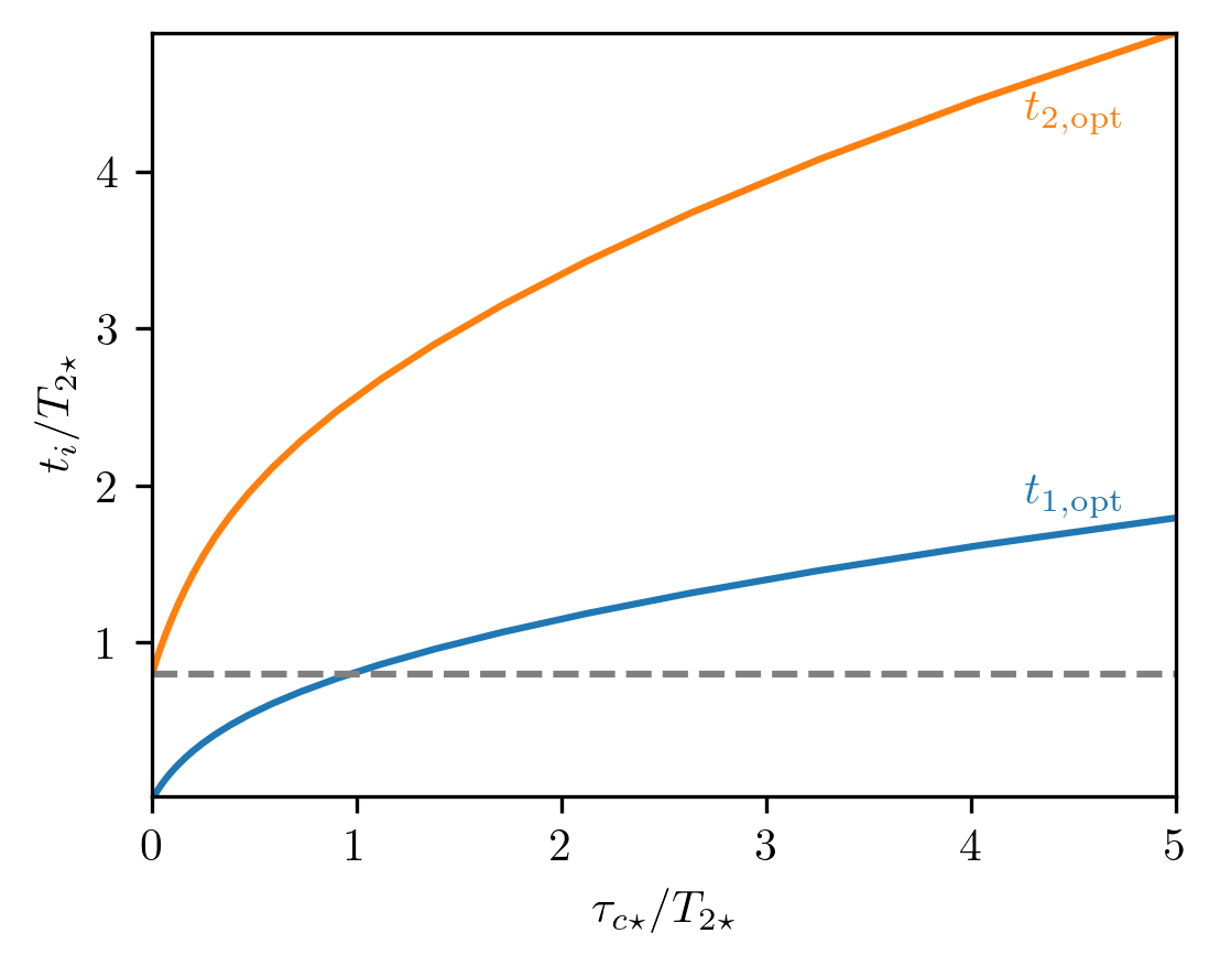
Figure 4: Optimal times for OU dephasing L$\ell$QT: We represent $(t_{1,\rm opt},t_{2,\rm opt})=\texttt{argmin}\{\det(\Sigma(t_{1},t_{2}))\}$ as a function of the ratio of the real noise parameters $\tau_{\rm c\star}/T_{2\star}$. In the regime where $\tau_{\rm c\star}\ll T_{2\star}$, we find that $t_{2}\approx 0.8T_{2\star}$ and $t_{1}\approx 0$. The optimal time of this measurement lies very close to the Lindbladian result $t=0.797T_{2\star}$ found when there is no time correlation and we have a single parameter $T_{c}$, which is an exact analytical result discussed in App. B.

Bayesian Ramsey estimators.

Let us now describe how a Bayesian inference for OU dephasing L$\ell$QT would proceed, which will provide an experimental procedure to operate at the optimal estimation times. We start by commenting on the fully-uncorrelated Lindbladian limit discussed in App. B, where the optimization of the measurement time for each Bayesian step (37) can also be solved analytically. Considering that the prior probability distribution $\pi_{\ell}(\gamma)$ for our knowledge about the decay rate at the $\ell$-th step is Gaussian, we can focus on how its mean and variance change as one takes the next Bayesian step. In the Appendix, we show that, minimizing the Bayesian variance (68) of the next step, one finds optimal measurement times that agree with the above frequentist prediction, albeit for the knowledge of the decay rate that we actually have at each particular step $t_{\ell}=0.797/2\hat{\gamma}_{\ell}$ or, alternatively, of the decoherence time $T_{2,\ell}$. This result is very encouraging, as the experimentalist may only have a crude guess of this value, but it gets automatically updated towards the optimal regime. This motivates an extension to time-correlated dephasing such as the OU noise.

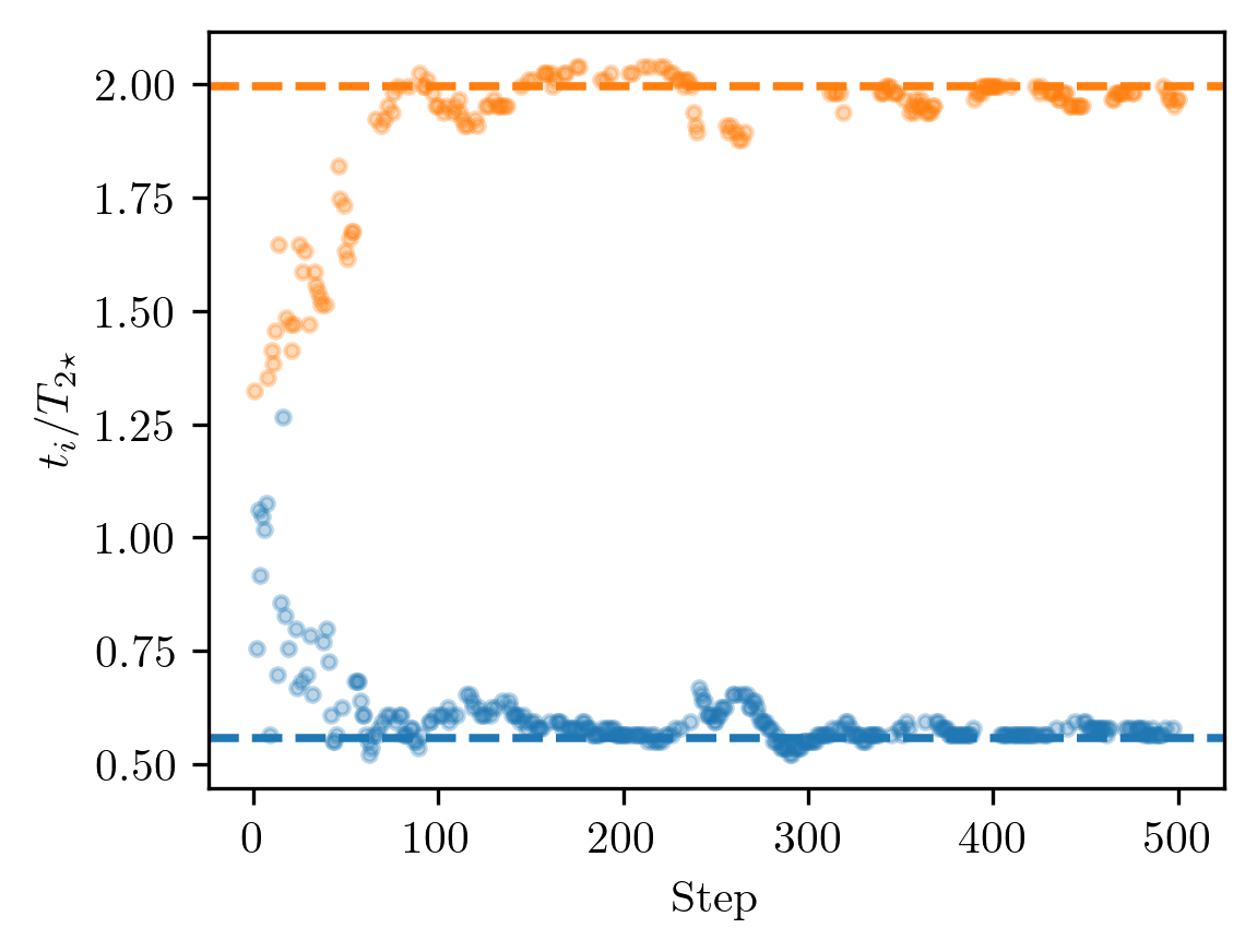
Figure 5: Bayesian optimal measurement time at each step: We consider OU noise and set $\tau_{\rm c\star}=T_{2\star}/2$. The prior of the parameters is a continuous uniform distribution with $T_{2}\in[T_{2\star}/3,3T_{2\star}],\tau\in[\tau_{\rm c\star}/3,3\tau_{\rm c\star}]$. At each Bayesian step, we increase the data set with $|\delta\mathbb{D}_{\ell}|=50$ new outcomes, which are used to compute the Bayesian update. The total number of measurements after 500 steps is $500\times 50=25000$. In the Bayesian steps at the beginning, we see that the evolution times lie around $t\sim T_{2\star}$. Later on, the algorithm tends to alternate between two times, which correspond to the optimal times $t_{1,\rm opt}\approx 0.56T_{2\star}$, $t_{2,\rm opt}\approx 1.99T_{2\star}$ in the case of $\tau_{\rm c\star}=T_{2\star}/2$. As the number of steps increases and and the posterior gets closer to the true values of $\tau_{\rm c\star}$ and $T_{2\star}$, the Bayesian algorithm tends to select measurement times which are closer to the optimal times.

For the OU dephasing, we have two parameters to learn, and we can maximize the Kullback-Leibler divergence (37) to obtain the subsequent optimal time $t_{\ell}$ for the next Ramsey measurement(s), and the corresponding extension of the data set $\mathbb{D}_{\ell-1}\mapsto\delta\mathbb{D}_{\ell}=\mathbb{D}_{\ell-1}\cup\delta\mathbb{D}_{\ell-1}$. We then proceed by measuring at this time, updating the prior, and starting the optimization step all over again to finally find the estimates (35) $\bm{\hat{\theta}}_{{\rm B}}=(\hat{\tau}_{{\rm c},\ell},\hat{T}_{2,\ell})$. As shown in Fig. 5, as one collects more and more data, the Bayesian measurement times cluster at two single times, and tend to alternate between them. Remarkably, these times are the optimal $t_{1,{\rm opt}}$ and $t_{2,{\rm opt}}$ predictions of the frequentist approach shown in Fig. 4. We can see how the Bayesian approach automatically finds the optimal measurement setting to learn a time-correlated dephasing noise.

Let us now present a detailed comparison of the precision of the frequentist and Bayesian approaches. For the frequentist approach, we can obtain the expected covariance of the estimator ${\rm Cov}(\bm{\hat{\theta}}_{\rm F})$ by performing several runs, and computing the covariance matrix of the results. We emphasise that this is not the asymptotic $\Sigma_{\bm{\hat{\theta}}}$ discussed previously, and does not require a very large number of measurement shots. For the Bayesian approach we obtain a posterior probability distribution after $\ell$ steps, $\pi_{\ell}(\bm{\theta})$, and we can directly compute the covariance matrix $\Sigma_{\ell}$ of this posterior distribution. A good measure of the uncertainty of each one of the approaches can be obtained by taking the determinant of the corresponding covariance matrix. For a Gaussian distribution, this quantity $\det\Sigma$ gives us the elliptical area associated to the bi-variate Gaussian covariance, and we can define an average radius $\bar{R}=\sqrt{\det\Sigma}/\pi$. In order for this to scale as $1/\sqrt{N_{\rm shot}}$ and that it has the same units as the standard deviation, we will use the square root of this radius $\det\Sigma^{1/4}$. Therefore, we will compare $\det\Sigma^{1/4}$ for both frequentist and Bayesian approaches by taking the ratio of the determinants,

$$r_{\rm OU}=\sqrt[4]{\frac{\det(\mathrm{Cov}(\hat{\bm{\theta}}_{F,\mathrm{opt}}))}{\det\Sigma_{\ell_{\rm max}}}},$$ (45)

with $\hat{\bm{\theta}}_{F,\mathrm{opt}}$ the frequentist estimator taking measurements at optimal times and considering for both approaches the same number of total measurements $N_{\mathrm{shot}}$. This ratio is represented in Fig. 6 as a function of $\tau_{\rm c,\star}/T_{2\star}$. As we can see, the Bayesian approach is better for small number of measurements, since it has some prior knowledge of the parameters. As we make more measurements and the frequentist estimator keeps measuring at optimal times we get to the opposite situation. Finally, in the limit of big $N_{\mathrm{shot}}$ the Bayesian approach takes also most measurements at these optimal times and the ratio saturates to $r_{\mathrm{OU}}\approx 1$, indicating that both approaches offer a similar precision. Let us emphasize, however, that the frequentist approach will not operate in practice at the optimal times, as these depend on the noise parameters one aims at estimating. It is also interesting to note that, as the correlation time of the noise increases, the region where the Bayesian strategy overcomes the frequentist one grows also in terms of the required number of shots. In regimes in which the time correlations are much larger than the effective decoherence time, the Bayesian approach will always be preferred unless one can perform a prohibitively-large number of measurements.

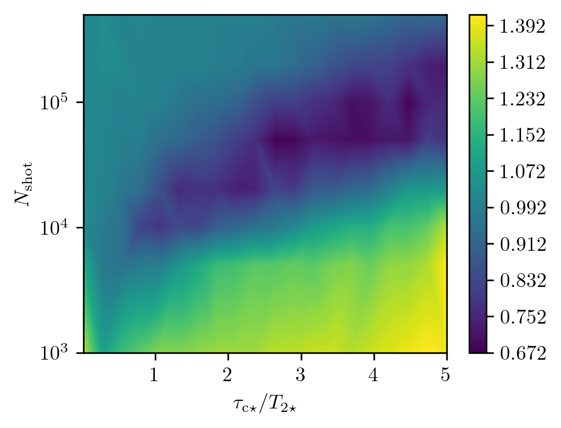
Figure 6: Comparison of frequentist and Bayesian approaches for OU noise: The ratio of Eq. (45) computed for different parameter values $\tau_{\mathrm{c}\star}$ and total number of shots $N_{\rm shot}$. 5000 frequentist runs were done to estimate $\det\mathrm{Cov}(\hat{\bm{\theta}}_{\mathrm{F,opt}})$, while 200 Bayesian runs were done to estimate $\det\Sigma_{\ell_{\rm max}}$ for each point $(\tau_{\rm c,\star},N_{\rm shot})$. In the Bayesian approach 100 shots were taken at each step and the prior is a continuous uniform distribution with $T_{2}\in[T_{2\star}/3,3T_{2\star}],\tau\in[\tau_{\rm c\star}/3,3\tau_{\rm c\star}]$. Analogously, for the least-squares minimization algorithm used in the frequentist approach (trust-region reflective algorithm), we set the same parameter bounds as the ones of the uniform distribution.

III.3.2 Non-Markovian quantum dephasing

Let us now move on to the discussion of L$\ell$QT for a non-Markovian dephasing dynamics. In the previous section, we have shown that a semi-classical dephasing with OU noise, an archetype for time-correlated Gaussian random processes, yields a dephasing map that, although departing from the time-homogeneous Lindbladian case, does not fall under the class of non-Markovian quantum dynamical maps. We have shown how both the frequentist and Bayesian approaches can learn the time-local master equation, which is parametrized in terms of an effective decoherence time $T_{2}$ and a correlation time $\tau_{\rm c}$. In this section, we focus on a quantum-mechanical dephasing noise that can actually lead to non-Markovianity in the qubit evolution, and see how the degree of non-Markovianity affects the precision of both the frequentist and L$\ell$QT.

We consider an apparently mild modification of the noise PSD with respect to the OU case (39). In particular, we use

$$S(\omega)=4g^{2}_{\bar{n}}\frac{\kappa}{(\omega+\Delta_{\rm c})^{2}+(\kappa/2)^{2}},$$ (46)

which is a Lorentzian of width $\kappa$ centered around $-\Delta_{\rm c}$, and reaching a maximum of $16g_{\bar{n}}^{2}/\kappa$. We note that for $\Delta_{\rm c}=0$, we recover the previous OU case (39) with $\tau_{\rm c}=2/\kappa$ and $c=4g^{2}_{\bar{n}}\kappa$. On the other hand, for $\Delta_{\rm c}\neq 0$, this PSD is not an even function $S(\omega)\neq S(-\omega)$, and the associated frequency noise cannot arise from a semi-classical stochastic model [113]. Instead, this particular PSD can be deduced from a quantum-mechanical dephasing model as discussed in App. A, and applied to a qubit coupled to a dissipative bosonic mode.

In the context of superconducting circuits [114], $\Delta_{\rm c}$ is the detuning of a bosonic microwave resonator with respect to the frequency of an external driving, which is considered to be resonant with the qubit, such that $\Delta_{\rm c}=\omega_{\rm c}-\omega_{0}$. In addition, $g$ is a qubit-resonator cross-Kerr coupling that leads to a bosonic enhancement $g^{2}_{\bar{n}}=g^{2}\bar{n}$, where $\bar{n}$ is the average bosonic occupation of the driven resonator, and $\kappa$ is the rate of spontaneous emission/loss of photons into the electromagnetic environment. We note that a similar dynamics can be engineered in a two-ion crystal, in analogy to [115], such that one of the ions encodes the qubit in a pair of ground state/metastable levels, while the other one is continuously Doppler cooled via a laser that is red-detuned with respect to a dipole-allowed transition. This laser then drives the carrier and motional sidebands, and effectively laser cools the common vibrational modes, one of which will play the role of the above dissipative bosonic mode, such that the above $\omega_{\rm c}$ will now be its vibrational frequency. The role of the above $\kappa$ is then played by the laser cooling rate, and the phonon population in the steady state $\bar{n}$ depends on the difference of laser cooling and heating processes [116], which can be controlled by the Rabi frequency and detuning of the laser that drives the dipole-allowed transition. The dissipative phonons will then act as an effective Lorentzian bath for the qubits [115, 117, 118]. We consider the qubit to be subjected to a far-detuned sideband coupling, which induces a second-order cross-Kerr coupling of strength $g$ describing a phonon-dependent ac-Stark shift on the qubit levels.

In any of the two architectures discussed, when the coupling between the bosonic mode and the qubit is weaker than the dissipative rate $g_{\bar{n}}\ll\kappa$, one can truncate the cumulant expansion of a time-convolutionless master equation of the qubit at second order such that, after tracing over the driven-dissipative mode in its stationary state, one arrives at a time-local dephasing master equation of the form (12). This master equation will be controlled by an auto-correlation function (63) for the bath operator $B(t)=2g(a^{\dagger}a-\bar{n})$, following the notation used below Eq. (13) and in App. A. In particular, making use of the quantum regression theorem [119], this auto-correlation can be expressed as

$$C(t-t^{\prime})=4g^{2}_{\bar{n}}\mathord{\rm e}^{-\frac{\kappa}{2}|t-t^{\prime}|}\mathord{\rm e}^{-\mathrm{i}\Delta_{\rm c}(t-t^{\prime})},$$ (47)

which coincides with the OU auto-correlation function (38) when $\Delta_{\rm c}=0$. Being wide-sense stationary, one can Fourier transform this function (14), leading to the displaced Lorentzian PSD in Eq. (46). Following Eq. (15), one can obtain the following time-dependent decay rate

$$\gamma(t)=\frac{1}{4}S(0)\left(1-\mathord{\rm e}^{-\frac{\kappa}{2}t}\Bigr{(}\cos\Delta_{\rm c}t+\frac{2\Delta_{\rm c}}{\kappa}\sin\Delta_{\rm c}t\Bigl{)}\right).$$ (48)

In comparison to Eq. (40), this decay rate presents additional oscillatory terms for $\Delta_{\rm c}\neq 0$ that will play an important role for the non-Markovianity of the quantum dynamical map. The attenuation factor that controls the decay of the coherence is

$$\Gamma(t)= \frac{S(0)}{2}\bigg{(}t+\frac{2_{\phantom{{}_{c}}\!\!}}{\kappa_{\phantom{{}_{c}}\!\!}}\frac{(2\Delta_{\rm c}/\kappa)^{2}-1}{(2\Delta_{\rm c}/\kappa)^{2}+1}+\frac{2}{\kappa}\mathord{\rm e}^{-\frac{\kappa}{2}t}\cos\varphi(t)\bigg{)},$$ (49)

where we have introduced $\varphi(t)=\Delta_{\rm c}t-2\arctan\frac{2\Delta_{\rm c}}{\kappa}$.

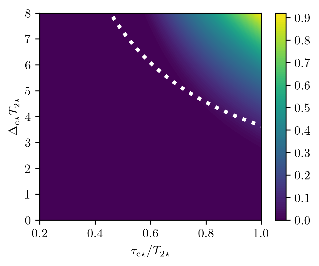
Figure 7: Non-Markovianity measure for the quantum dephasing map: non-Markovianity measure of Eq. (24) for different values of $\tau_{c}=2/\kappa$ and $\Delta_{\rm c}$. The dashed line signals the limit between the Markovian and the non-Markovian regions and corresponds to the equation $\Delta_{\rm c}\approx 1.82\kappa$.

Recalling that we can assign a correlation time to this noise by $\tau_{\rm c}=2/\kappa$, one would expect to recover a Markovian Lindbladian description for $t\gg\tau_{\rm c}$. In this limit, the term linear in $t$ in Eq. (49) is the dominant one, which leads to a time-homogeneous exponential decay of the Ramsey probabilities $p^{\rm TL}_{i}(m_{x}|\bm{\theta})\approx\big{(}1+(-1)^{m_{x}}\mathord{\rm e}^{-t_{i}/T_{2}}\big{)}/2$ with an associated decoherence time $T_{2}=2/S(0)=({(\kappa/2)^{2}+\Delta_{\rm c}^{2}})/{2g^{2}_{\bar{n}}\kappa}$. As in the OU case, for shorter times, the memory effects will start playing a bigger role in the qubit dynamics, such that the Ramsey decay is no longer a time-homogeneous exponential. Moreover, in this particular case, these memory effects can give rise to a non-Markovianity that can be understood as a backflow of information from the environment into the system. According to Eq. (24) or (25), non-Markovianity occurs when the decay rate takes negative values $\gamma(t)<0$. This can only happen if the second contribution in Eq. (48) dominates over the first one, which cannot happen if $\Delta_{\rm c}=0$. Since this contribution is suppressed by $\mathord{\rm e}^{-\kappa t/2}$, we will need the frequency of the oscillations $\Delta_{\rm c}$ to be sufficiently large in comparison to $\kappa$, such that one can get a non-vanishing degree of non-Markovianity. In Fig. 7, we depict the measure of non-Markovianity of Eq. (24) as a function of $\Delta_{\rm c}$ and $\tau_{\rm c}=2/\kappa$. We see that the parameter regime $\Delta_{\rm c}\gtrsim 1.82\kappa$ (white dashed line) is where $\gamma(t)$ can become negative at some time during the evolution, leading to larger non-Markovianity as both $\Delta_{\rm c}$ and $\tau_{\rm c}$ are further increased.

Let us now discuss the statistical inference for the L$\ell$QT of this non-Markovian dephasing map, and compare the frequentist and Bayesian approaches to the statistical estimation.

Frequentist Ramsey estimators.

As in the OU case, we need to minimize $\mathsf{C}^{\rm pd}_{\mathrm{TL}}(\bm{\theta})$ in Eq. (26), where the likelihood function $p^{\rm TL}_{i}(m_{x}|\bm{\theta})=\big{(}1+(-1)^{m_{x}}\mathord{\rm e}^{-\Gamma(t_{i})}\big{)}/2$ now depends on the new attenuation factor (49). Since there are three noise parameters $\bm{\theta}_{\star}=(g^{2}_{\bar{n}\star},\kappa_{\star},\Delta_{{\rm c}\star})\in\Theta=\mathbb{R}^{3}_{+}$, we shall at least need to measure at three different times. To assess the performance of the frequentist approach under shot noise, we numerically generate the relative frequencies $\tilde{f}_{1}(m_{x}\,|\bm{\theta}_{\star}),\tilde{f}_{2}(m_{x}\,|\bm{\theta}_{\star}),\tilde{f}_{3}(m_{x}\,|\bm{\theta}_{\star})$ at these times by sampling the probability distribution with the real noise parameters $\bm{\theta}_{\star}$ a number of times $N_{\rm shot}=N_{1}+N_{2}+N_{3}$. In order to find the three optimal times, we minimize the determinant of the covariance matrix (44), which will have an similar expression as Eq. (43), but now expressed in terms of $3\times 3$ matrices for the underlying trivariate normal distribution. Since we are optimizing $t_{1}$, $t_{2}$ and $t_{3}$, one may wonder if we also could improve the estimation by redistributing the total number of measurements differently at each of these times. However, according to our prescription in which the imprecision is quantified by the long-run Gaussian pdf, which defines an elliptical volume in this case, one gets $\det\Sigma_{\bm{\hat{\theta}}}(t_{1,\rm opt},t_{2,\rm opt},t_{3,\rm opt})\propto{1}/{N_{1}N_{2}N_{3}}$. Therefore, the number of measurements must be equally distributed between the three different times $N_{1}=N_{2}=N_{3}=N_{\rm shot}/3$.

The minimization in Eq. (44) then yields the optimal times $\{t_{1,{\rm opt}},t_{2,{\rm opt}},t_{3,{\rm opt}}\}$ shown in Fig. 8, which have been represented as a function of $\tau_{{\rm c}\star}/T_{2\star}$ for a fixed value of $\Delta_{\rm c\star}$. The non-zero value of the later is responsible for the fact that, for $\tau_{{\rm c}\star}\gtrsim 0.73T_{2\star}$, we cross the red-dashed line and enter a non-Markovian regime in which the effective dephasing dynamics is no longer CP-divisible. In this non-Markovian regime, the optimal times tend to be close to the local maxima of $\tilde{f}_{i}(m_{x}|\bm{\theta}_{\star})$, providing a large amount of information about the dephasing noise. Conversely, deep in the Markovian regime $\tau_{\rm c\star}\ll T_{2\star}$, it suffices to measure at $t_{3,{\rm opt}}\approx 0.797T_{2\star}$ in order to determine $T_{2\star}$, in agreement with the analytical Lindblad result, while $t_{1,{\rm opt}}$ and $t_{2,{\rm opt}}$ tend to zero and would be used to determine the two other noise parameters.

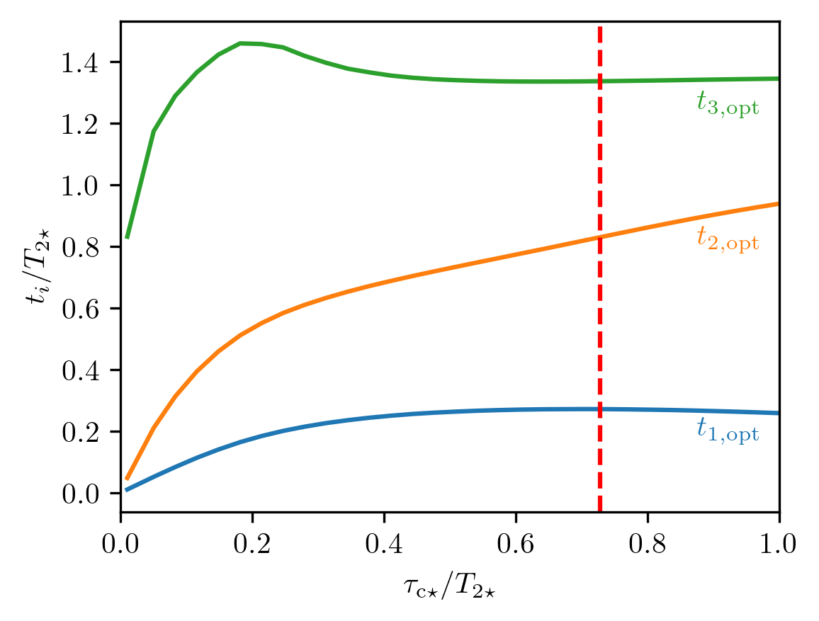
Figure 8: Optimal times for quantum dephasing L$\ell$QT: We represent the three optimal times $(t_{1,\rm opt},t_{2,\rm opt},t_{3,\rm opt})=\texttt{argmin}\{\det(\Sigma_{\bm{\hat{\theta}}}(t_{1},t_{2},t_{3}))\}$ as a function of the ratio of the real noise parameters $\tau_{\rm c\star}/T_{2\star}$, setting $\Delta_{{\rm c}\star}=5/T_{2\star}$. The vertical red dashed line separates the Markovian regime (left) from the non-Markovian one (right). On the Markovian regime, as $\tau_{{\rm c}\star}\ll T_{2\star}$, we see that the $t_{1},t_{2}$ in blue and orange tend to zero, while $t_{3}$ in green tends to the optimal value of the pure Lindbladian case $t_{3}\approx 0.797T_{2\star}$. On the other hand, as $\tau_{{\rm c}\star}$ increases and memory effects become more relevant, the three optimal times start to depart from each other. In the non-Markovian regime, the optimal time $t_{2,\rm opt}$ is closer to $t_{3,\rm opt}$ than it is to $t_{1,\rm opt}$. Moreover, this optimal $t_{1,\rm opt}$ time starts to decrease as $\tau_{{\rm c}\star}$ goes deep into the non-Markovian regime.

Bayesian Ramsey estimators.

Let us now move to the Bayesian approach, where we have some prior knowledge (34) of the parameters $\bm{\theta}=(g^{2}_{\bar{n}},\kappa,\Delta_{\rm c})$ that gets updated at each Bayesian step $t_{\ell}$ by enlarging the data set with $\delta\mathbb{D}_{\ell}$. Minimizing the relative entropy between the prior and the posterior (37), we obtain the subsequent evolution time $t_{\ell}$, and update our knowledge about the noise parameters in the best possible way. As shown in Fig. 9, the Bayesian procedure starts by using evolution update times that are scattered in a broad range of values. However, as the number of iterations increases and we gain more knowledge, they tend to cluster around three well-defined times. In fact, as shown by the corresponding dashed lines, these times coincide with the optimal measurement times of the frequentist approach in Fig. 8. Therefore, if we start a Bayesian experiment with some prior, and we let the experiment run for sufficiently long number of steps, we will learn the optimal times automatically.

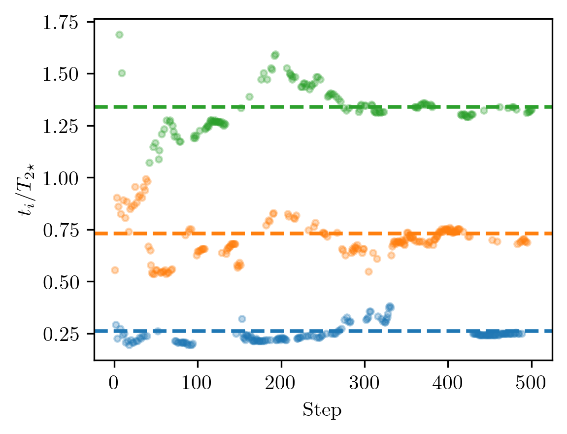
Figure 9: Bayesian optimal measurement time at each step: We consider the non-Markovian quantum dephasing with noise parameters $\tau_{\rm c,\star}=T_{2\star}/2$ and $\Delta_{\rm c\star}=5/T_{2\star}$. We consider as initial prior a continuous uniform distribution with $g_{\bar{n}}^{2}\in[g_{\bar{n}\star}^{2}/3,3g_{\bar{n}\star}^{2}],\kappa\in[3\kappa_{\star},\kappa_{\star}/3],\Delta_{\rm c}\in[3\Delta_{\rm{c}\star},\Delta_{\rm{c}\star}/3]$. At each Bayesian step, we increase the data set with $|\delta\mathbb{D}_{\ell}|=50$ new outcomes. As the Bayesian protocol proceeds, we see that the Bayesian update times cluster in three groups of data, which lie around the optimal times $t_{1,{\rm opt}},t_{2,{\rm opt}},t_{3,{\rm opt}}$ of the frequentist approach, which are represented by dashed lines.

In order to compare the precision of the frequentist and Bayesian approaches, we proceed in analogy to the OU noise by looking for a parameter that captures the relative precision of the two approaches (45). We now have to consider that the determinant of the trivariate Gaussian covariance $\det\Sigma$ is a volume, and we can define an average radius as $\bar{R}=\sqrt[3]{\det\Sigma}/(4\pi/3)$. We can quantify the precision by taking the square root of this radius, which scales like a standard deviation. Altogether, the relative precision of the frequentist and Bayesian approaches is defined by the ratio

$$r_{\rm NM}=\sqrt[6]{\frac{\det(\mathrm{Cov(\hat{\bm{\theta}}_{\mathrm{F,opt}})})}{\det\Sigma_{\ell_{\rm max}}}}.$$ (50)

Here, $\hat{\bm{\theta}}_{F,\mathrm{opt}}$ is the frequentist estimator taking measurements at the optimal times, and we consider the same number of total measurements $N_{\mathrm{shot}}$ for both approaches. This ratio is represented in Fig. 10 for $N_{\rm shot}=2\times 10^{4}$, which is still far from the asymptotic regime of large $N_{\rm shot}$ where one would obtain $r_{\rm NM}\approx 1$ in similarity to the results found for the OU noise in Fig. 6. Instead of exploring how this ratio changes with the number of measurement shots, we are here interested in understanding how the degree of non-Markovianity can affect the performance of the two estimation strategies. We thus set $N_{\rm shot}=2\times 10^{4}$, since the variance is already good enough but the cost in terms of number of measurements is still not too big, and plot the precision ratio as a function of the real noise parameters. As we can see in Fig. 10, the blue region represents a regime in which the frequentist approach is slightly better than the Bayesian one, and coincides with the regime of Markovian dephasing that is delimited by the dashed white line. The continuous white line marks the ratio contour line with $r_{\rm NM}=1$, and thus delimits the part of the blue region in which the frequentist approach with optimal times is preferable. In the green and yellow areas, which coincide with the non-Markovian regime, the Bayesian approach becomes preferable and the advantage can actually be quite significant. As we go deeper in the non-Markovian regime, the oscillating term in Eq. (49) becomes bigger and the decay of the coherence exhibits an increasing number of local maxima. These local maxima represent times that provide a significant amount of information in terms of the Kullback-Leibler divergence of Eq. (37). Therefore, the presence of more local maxima in the non-Markovian regime makes it easier for the Bayesian method to, even if the prior information is minimal, select a time as useful as the asymptotically optimal times.

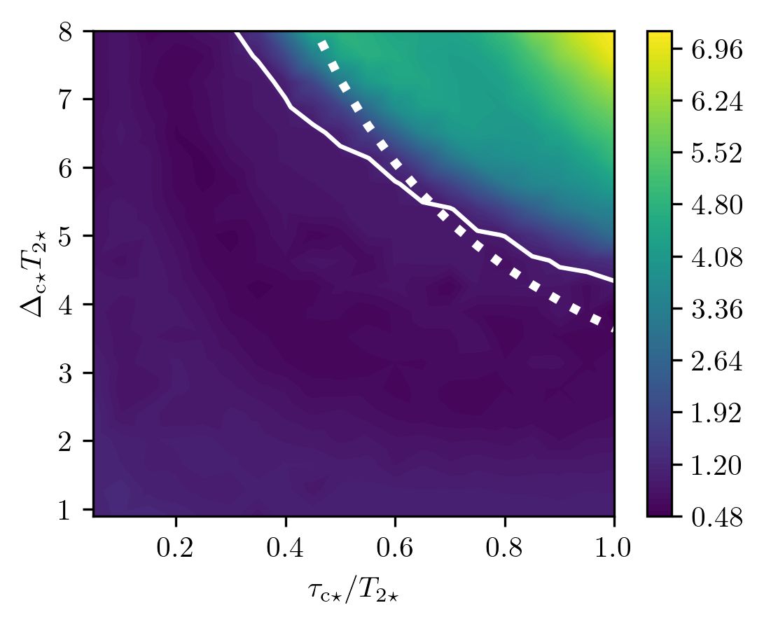
Figure 10: Ratio between determinants of covariance matrices of frequentist and Bayesian approaches: The ratio of Eq. (50) computed for different parameter values $\tau_{\mathrm{c}\star}$ and $\Delta_{\mathrm{c}\star}$, and a fixed number of total measurements $N_{\rm shot}=2\cdot 10^{4}$. The dashed white line separates the Markovian from the non-Markovian regime. The continuous white line indicates the level where the ratio equals 1. 5000 frequentist runs were done to estimate $\det\mathrm{Cov(\hat{\bm{\theta}}_{\mathrm{F,opt}})}$, while 30 Bayesian runs were done to estimate $\det\Sigma_{\ell_{\rm max}}$ for each point $(\tau_{\rm c\star},\Delta_{\rm c\star})$. In the Bayesian approach 100 shots were taken at each step and the prior is a continuous uniform distribution with $\bm{\theta}\in[\bm{\theta}_{\star}/3,3\bm{\theta}_{\star}]$. Analogously, for the least-squares minimization used in the frequentist approach (trust-region reflective algorithm), we set the same parameter bounds as the ones of the uniform distribution.

It is also useful to quantify the advantage of one estimator with respect to the other in terms of number of measurements that is required to reach a target precision, which amounts to reaching the same value of the above covariance determinant. The values shown for the ratio of the determinants in Fig. 10 can be converted into the ratio of number of measurements by assuming that both covariance determinants in Eq. (50) scale as $1/\sqrt{N_{\rm shot}}$ even in the non-asymptotic regime. Although there can be corrections to this scaling, this can give us in most cases an idea of the proportion of measurement shots one can save by using the best estimator. With this assumption, we get $N_{\rm shot,F}/N_{\rm shot,B}\approx r_{\rm NM}^{2}$, with $r_{\rm NM}$ the ratio of the determinants of two different approaches. Thus, if for instance $r_{\mathrm{\rm NM}}=1.5$, we obtain that $N_{\rm shot,F}/N_{\rm short,B}\approx 2.25$. Therefore, we get more than a $2\times$ reduction in the number of measurements with the Bayesian approach in comparison to the frequentist one to reach the same precision. Going back to the values of Fig. 10, we see that the Bayesian approach can result in a considerable improvement as one goes deep in the non-Markovian limit. Before closing this subsection, it is worth recalling once more that, in practice, the frequentist estimation will never be performed at the three optimal times, and the advantage of the Bayesian approach can even be bigger. In App. C, we present a detailed comparison of these estimators with another one in which the shots are evenly distributed between the measurements after evolution times that cover uniformly the whole time interval $T$. As discussed in the appendix, the Bayesian approach is preferable for most of the parameter values, and can again show a big advantage as one enters into the non-Markovian regime.

IV Conclusions and outlook

We have presented L$\ell$QT, a new tool designed to characterize non-Markovian dephasing noise in QIPs. Building upon the established framework of Lindblad quantum tomography, L$\ell$QT extends the applicability of Lindblad learning to scenarios where temporal correlations and non-Markovian dynamics play a significant role. In particular, it allows us to extend the characterization of the generators of quantum dynamical maps that go beyond the time-homogeneous Lindblad limit, which connect to a time-local master equation that can display negative decay rates in certain time intervals and, thus, strictly non-Markovian quantum evolutions. Through a detailed comparative study, both frequentist and Bayesian approaches to L$\ell$QT are presented, offering insights into the accuracy and precision of noise estimation under different conditions.

By focusing on the time-correlated dephasing quantum dynamical map of a single qubit, we show that L$\ell$QT can be formally expressed as a parameter estimation process, which simplifies the most general learning scheme to a single initial state and a single measurement basis. In particular, the problem reduces to a time-correlated Ramsey estimator for a parametrized decay rate, which depends on the noise parameters via a filtered power spectral density of the noise. In the frequentist approach, the focus lies on optimizing measurement times to reduce the number of necessary measurements while minimizing error in parameter estimation. By leveraging statistical inference techniques, the frequentist approach provides valuable insights into the efficiency and effectiveness of L$\ell$QT, particularly in scenarios with varying degrees of temporal correlations and non-Markovianity. Conversely, the Bayesian approach offers a more dynamic and adaptive framework, allowing for the incorporation of prior knowledge and iterative updates to refine noise estimates over time.

We have compared the performance of both approaches for two different dephasing quantum dynamical maps, either for a semi-classical or for a quantum-mechanical noise model. In both cases, the microscopically-motivated parametrization allows one to interpolate between a fully Markovian Lindblad limit, for which we derive analytical solutions for the optimal estimation, and a time-correlated and even non-Markovian regime which require a different distribution of the optimal and Bayesian measuring times. Interestingly, in the quantum-mechanical dephasing model, which can be obtained from a microscopic model of a qubit that is coupled to a dissipative bosonic mode in both superconducting-circuit and trapped-ion architectures, the best of the two approaches depends on whether we are in the Markovian or the non-Markovian regime. The Bayesian approach yields much better results in the non-Markovian regime, showing that it is able to automatically adapt to the particularities of the non-Markovian evolution to make much better estimations with a limited number of shots. Moreover, we also compare to more standard schemes considered in the context of Lindbladian quantum tomography, in which the measurements are distributed uniformly, showing an advantage of our schemes that again becomes more appreciable in the non-Markovian regime.

Future research shall explore the extension of these non-Markovian characterization techniques to larger quantum systems, combining the effect of spatial and temporal correlations. More importantly, our work sets the stage to generalize to more complex situations beyond pure dephasing, specially focusing on scalability and robustness, and eventually targeting the noise in full universal gate sets of QIPs.

Appendix A Time-local master equation for pure dephasing

For the sake of completeness, we present here a derivation of the time-local master equation (12) for a qubit subjected to time-correlated dephasing noise, both in a semi-classical and a fully quantum-mechanical model. This serves to introduce well-known concepts and set our notation following [77].

Semi-classical time-correlated dephasing.-

The qubit evolves under a stochastic rotating-frame Hamiltonian

$$\tilde{H}(t)=\frac{1}{2}\delta\tilde{\omega}(t)\sigma_{z},$$ (51)

where $\delta\tilde{\omega}(t)$ is the detuning of the qubit with respect to the frequency of a driving used in the initialization/measurement stages with respect to, and we have set $\hbar=1$. We use a tilde to highlight the random nature of $\delta\tilde{\omega}(t)$, which is modeled as a stochastic process with zero mean $\mathbb{E}[\delta\tilde{\omega}(t)]=0$, thus assuming that the driving frequency is resonant with the qubit transition on average. We recall that the averages are taken with respect to the underlying joint probability density function (pdf) of the process for any finite set of times $p_{\delta\tilde{\omega}}(\delta\bm{\omega})=p_{t_{1},t_{2},\cdots,t_{n}}(\delta\omega_{1},\delta\omega_{2},\cdots,\delta\omega_{n})$, $\forall n\in\mathbb{Z}^{+}:\delta\omega_{n}=\delta\omega(t_{n})\in\mathbb{R},\,\{t_{i}\}_{i=1}^{n}\in T$, which fulfills the conditions $p_{\delta\tilde{\omega}}(\delta\bm{\omega})\geq 0$ and $\int\prod_{n}{\rm d}\delta\omega_{n}p_{\delta\tilde{\omega}}(\delta\bm{\omega})=1$  [120, 111]. Physically, these stochastic fluctuations can either stem from frequency/phase noise of the drive, or from additional external fields that shift the energy of the qubit. For each individual trajectory of the noise $\delta\tilde{\omega}(t)$, the evolution of an initial qubit state $\rho_{0}=\ket{\psi_{0}}\!\bra{\psi_{0}}$ in the rotating frame is purely unitary but random, giving rise to $\tilde{\rho}(t)$, and expectation values will thus depend on stochastic averages $\mathbb{E}$, leading to a completely-positive trace-preserving (CPTP) map after averaging $\rho(t)=\mathbb{E}[\tilde{\rho}(t)]=\mathcal{E}_{t,t_{0}}({\rho}_{0})$ [1, 121, 122, 64]. The corresponding stochastic differential equations are

$$\frac{\rm d\tilde{\rho}}{{\rm d}t}=\tilde{\mathcal{L}}_{t}(\tilde{\rho}(t)),\hskip 4.30554pt\tilde{\mathcal{L}}_{t}(\bullet)=-\mathord{\rm i}[\tilde{H}(t),\bullet\,],$$ (52)

where one sees that the noise $\delta\tilde{\omega}(t)$ thus enters multiplicatively. Using the Nakajima-Zwanzig [74] projection operators $\mathcal{P}=\mathbb{E}$, and $\mathcal{Q}=1-\mathcal{P}$, we can find differential equations for the averaged density matrix using

$$\rho(t)=\mathcal{P}(\tilde{\rho}(t)):\hskip 8.61108pt\mathcal{Q}(\rho_{0})=0=\mathcal{P}(\tilde{\mathcal{L}}_{t}).$$ (53)

In fact, this averaged evolution can be written as a time-local master equation [91, 123, 124], namely

$$\frac{\rm d{\rho}}{{\rm d}t}=\mathcal{K}\!(t)\rho(t),$$ (54)

where $\mathcal{K}\!(t)$ is the so-called time-convolutionless kernel that encapsulates the effects that the finite memory of the time-correlated noise has on the qubit. In particular, this kernel can be expressed as follows

$$\mathcal{K}\!(t)=\mathcal{P}\tilde{\mathcal{L}}_{t}(1-\tilde{\Sigma}(t))^{-1},$$ (55)

where we have used a super-operator playing the role of a ‘self-energy’, which can be expanded as

$$\tilde{\Sigma}(t)=\sum_{m}\alpha^{m}\tilde{\Sigma}_{m}(t),\hskip 4.30554pt\mathcal{K}\!(t)\!=\sum_{n}\mathcal{P}\tilde{\mathcal{L}}_{t}\!\left(\!\sum_{m}\alpha^{m}\tilde{\Sigma}_{m}(t)\!\!\right)^{\!\!n}\!\!\!.$$ (56)

In this way, the kernel is organised in a power series of a microscopic coupling $\alpha$ that characterizes the order of magnitude of the coupling of the system to the external noise, and Eq. (53) can be used to show that only even terms contribute

$$\mathcal{K}\!(t)=\sum_{n}\mathcal{K}_{2n}(t).$$ (57)

This series agrees with the Kubo and Van Kampen cumulant expansion [125, 126], and one finds that the $n$-th order term can be expressed in terms of $n-1$ nested time-ordered integrals [127], being the lowest-order contribution $\mathcal{K}_{2}(t)=\int_{0}^{t}\!{\rm d}t^{\prime}\mathcal{P}(\tilde{\mathcal{L}}_{t}\tilde{\mathcal{L}}_{t^{\prime}})$. This term is controlled by the auto-correlation of the stochastic process, leading to

$$\frac{{\rm d}{\rho}}{{\rm d}t}=\frac{1}{4}\int_{0}^{t}\!{\rm d}t^{\prime}\left(C(t,t^{\prime})+C(t^{\prime},t)\right)\big{(}\sigma^{z}\rho(t)\sigma^{z}-\rho(t)\big{)},$$ (58)

which, for wide-sense stationary processes, can be expressed in terms of the PSD of the stochastic process

$$C(t-t^{\prime})=\mathbb{E}[\delta\tilde{\omega}(t)\delta\tilde{\omega}(t^{\prime})]=\int_{-\infty}^{\infty}\!\!\frac{{\rm d}\omega}{2\pi}\,S(\omega)\,\mathord{\rm e}^{\mathord{\rm i}\omega(t-t^{\prime})}.$$ (59)

We note that for any wide-sense stationary classical noise, the PSD is even $S(\omega)=S(-\omega)$ [113], and $C(t,t^{\prime})=C(|t-t^{\prime}|)=C(t^{\prime},t)$ such that the symmetrized autocorrelation function and the symmetrized PSD introduced below Eq. (16) already contain all of the required information for a second-order approximation. The truncation at this order is justified by first noting that the autocorrelation is typically concentrated within $|t-t^{\prime}|\leq{\tau}_{c}$, where ${\tau}_{\rm c}$ is a characteristic correlation time. Due to the cluster property [123, 128], one finds that $\mathcal{K}_{2}(t)\sim\alpha\zeta$ with $\alpha=\sqrt{C(0)}$ and a small parameter

$$\zeta=\alpha{\tau}_{\rm c}=\sqrt{\frac{\tau_{\rm c}}{T_{2}}},$$ (60)

where we have defined a characteristic time as $T_{2}=2/S(0)$. The cluster property for the higher $n$-th order contributions, which have $(n-1)$ nested integrals, states that the corresponding kernels scale with $\mathcal{K}_{n}(t)\sim\alpha\zeta^{n-1}$, justifying a low-order truncation whenever the condition $\zeta\ll 1$ is met. This is known as a fast-fluctuation expansion and, back from the rotating frame, yields the time-local master equation (12).

Before finishing this section of the Appendix, let us note that the above truncation rests on the importance of the memory effects $\tau_{\rm c}$ within the $T_{2}$ time. As discussed in more detail in the main text, this $T_{2}$ time controls the time scale for the decay of coherences $\langle\sigma_{x}(t)\rangle\approx\mathord{\rm e}^{-t/T_{2}}$ in a long-time Lindbladian limit $t\gg\tau_{\rm c}$. However, for shorter times, the structure of the noise can actually lead to deviations from this limit, leading to a coherence decay that is not exponential. As emphasized in the main text, this is not an univocal signal of non-Markovianity for the qubit evolution. We note that there is an exception to the $\tau_{\rm c}\ll T_{2}$ requirement for Gaussian random processes, which are defined by a joint pdf that is a multivariate normal distribution for any set of times. In this case, the time-local master equation (12) is actually an exact result, independently of the value of $\zeta$. In fact, the higher-order contributions to the kernel [74] vanish identically $\mathcal{K}_{n}(t)=0,\forall n>2$, due to Isserlis’ theorem, most commonly referred to as Wick’s theorem in the context of physics $\mathbb{E}[\delta\tilde{\omega}(t_{1})\delta\tilde{\omega}(t_{2})\cdots\delta\tilde{\omega}(t_{n})]=\sum_{\sigma\in S_{n}}\mathbb{E}[\delta\tilde{\omega}(t_{\sigma(1)})\delta\tilde{\omega}(t_{\sigma(2)})]\cdots\mathbb{E}[\delta\tilde{\omega}(t_{\sigma(n-1)})\delta\tilde{\omega}(t_{\sigma(n)})]$, where ${S}_{n}$ is the group of all possible permutations of $n$ elements, e.g. $\sigma(1,2,\cdots,n-1,n)=(n,1,2,\cdots,n-1)$.

Quantum-mechanical time-correlated dephasing.-

We consider a single qubit coupled to an environment, and evolving ${\rm d}\rho_{\rm SB}/{\rm d}t=\mathcal{L}_{t}(\rho_{\rm SB})$ under the following Liouvillian

$$\mathcal{L}_{t}=\mathcal{L}_{\rm SB}+\mathcal{L}_{\rm B},\hskip 4.30554pt\mathcal{L}_{\rm SB}(\bullet)=-\frac{\mathord{\rm i}}{2}\big{[}\big{(}\omega_{0}+B(t)\big{)}\sigma^{z},\bullet\big{]},$$ (61)

where $B(t)$ is an environment/bath operator that introduces fluctuations on the qubit frequency, and $\mathcal{L}_{\rm B}(\bullet)$ is the Liouvillian of the bath. In the standard description of quantum master equations, the environment is macroscopically large and subject to a purely-unitary evolution $\mathcal{L}_{\rm B}(\bullet)=-\mathord{\rm i}[H_{\rm B},\bullet]$. When the system-environment coupling is weak, one can assume that the environment remains unaltered, such that the evolution takes place on the qubit but there is no back action $\rho_{\rm SB}=\rho(t)\otimes\rho_{B}$. A Born-Markov approximation then yields a non-unitary master equation for the qubit [119]. This can be expressed as a time convolutionless master equation as the one discussed in the previous subsection (54), also truncated at second order, where $\mathcal{P}$ is now a super-operator tracing over the bath degrees of freedom $\mathcal{P}(\rho_{\rm SB})=\mathrm{Tr}_{B}(\rho_{\rm SB})=\rho$  [74]. The non-unitary evolution of the qubit results from the large number of degrees of freedom in the environment, such that the purity of the state can only decrease with no recurrences.

Let us note, however, that the conditions under which these assumptions are made can be more general, and the degrees of freedom playing the role of an environment need not be macroscopically large. The crucial requirement is that the time with which the effective environment reaches its steady state $\mathcal{L}_{\rm B}(\rho^{\rm ss}_{\rm B})=0$ must be much shorter than the timescale of interest in which the system evolves $\rho(t)$. In the present context, this is the case of a single bosonic mode that exchanges energy with a larger electromagnetic bath with a certain rate $\kappa$. The bath Liouvillian reads

$$\mathcal{L}_{\rm B}(\bullet)=-\mathord{\rm i}[\,H_{\rm B}(t),\bullet\,]+\kappa\left(a\rho a^{{\dagger}}-\textstyle\frac{1}{2}\{a^{{\dagger}}a,\bullet\}\right),$$ (62)

where $H_{\rm B}(t)$ is the bosonic mode Hamiltonian, which can include external drivings, and $a^{\dagger},a$ are the bosonic creation and annihilation operators, respectively. The condition for this single driven-dissipative mode to act as an environment is that $\kappa$ must be much larger than the coupling strength inside $B(t)$. In the context of the superconducting circuits discussed in the main text, $\kappa$ is the rate of photon loss in a resonator, and $H_{\rm B}$ must contain a linear resonant microwave driving of the resonator that controls the non-zero number of photons in the steady state [114]. For trapped ions, $\kappa$ will be the rate of sympathetic cooling of a vibrational model in a two-ion crystal, which will also be supplemented with a smaller heating rate  [116]. The difference of these two rates controls the population of phonons in the steady state, and can be controlled by an external laser.

We now move to the interaction picture with respect to the bare system Liouvillian $\rho_{I}(t)=\mathord{\rm e}^{t\mathcal{L}_{\rm S}}(\rho(t))$ with $\mathcal{L}_{\rm S}(\bullet)=-\mathord{\rm i}[\textstyle\frac{1}{2}\omega_{0}\sigma_{z},\bullet]$, and the bare bath Liouvillian, i.e., $B_{I}(t)=\mathord{\rm e}^{t\mathcal{L}_{\rm B}}(B(t))$. The key step is that, due to the fast decay of the bath, for the timescales of interest $t\gg 1/\kappa$, one can assume that $\rho_{\rm SB}(t)=\rho(t)\otimes\rho_{B}^{\rm ss}$, the second-order time-convolutionless master equation can be expressed as in Eq. (58) with

$$C(t,t^{\prime})=\big{\langle}B_{I}(t)B_{I}(t^{\prime})\big{\rangle}=\mathrm{Tr}_{B}\{B_{I}(t)B_{I}(t^{\prime})\rho_{\rm B}^{\rm ss}\}.$$ (63)

Here, we have assumed that $\mathcal{P}({B}_{I}(t))=0$, and we note that $B(t)$ need not commute with itself at different times. Once more, if these quantum-mechanical auto-correlation functions are wide-sense stationary, $C(t,t^{\prime})=C(t-t^{\prime})$. We note that, in contrast to the semi-classical case where $S(\omega)=S(-\omega)$, this is not necessarily the case in the quantum-mechanical case $S(\omega)\neq S(-\omega)$ [113]. However, in the case of pure dephasing, the time evolution (58) only depends on the symmetrized auto-correlation function $\bar{C}(t,t^{\prime})=\frac{1}{2}(C(t,t^{\prime})+C(t^{\prime},t))$ and therefore only the symmetric part of the auto-correlation function influences the time evolution

$$\frac{{\rm d}{\rho}}{{\rm d}t}=\frac{1}{2}\int_{0}^{t}\!{\rm d}t^{\prime}\bar{C}(t,t^{\prime})\big{(}\sigma^{z}\rho(t)\sigma^{z}-\rho(t)\big{)}.$$ (64)

Moving back to the Schrödinger picture, we obtain the master equation in Eq. (12), which will only depend on the symmetrized noise PSD defined below Eq. (16).

Appendix B Analytical results for the frequentist and Bayesian estimation of Markovian Lindblad dephasing

In this appendix, we provide an analytical solution of both the frequentist and Bayesian estimation for the LQT of single-qubit Lindblad dephasing. This serves to benchmark some of the limiting results of Sec. III.3. In the Lindblad approximation to pure dephasing, we can substitute $\gamma(t)=\gamma$ in Eq. (12), obtaining a constant dephasing rate. This leads to $\Gamma(t)=t/T_{2}$ in Eq. (18), where the dephasing time is $T_{2}=1/2\gamma$, such that the likelihood function $p^{\rm L}_{i}(m_{x}|T_{2})=\frac{1}{2}(1+(-1)^{m_{x}}\mathord{\rm e}^{-t_{i}/T_{2}})$ shows a purely-exponential coherence decay. Assuming that the actual qubit dephasing follows this pdf with a real value of $T_{2\star}$, or equivalently $\gamma_{\star}$, we have a single noise parameter to learn, and could thus estimate it by measuring at a single time $t_{i}=t$. Note that the relative frequencies in this case would follow $\tilde{f}_{i}(m_{x}|T_{2\star})=\frac{1}{2}(1+(-1)^{m_{x}}\mathord{\rm e}^{-t_{i}/T_{2\star}})$ for $N_{\rm shot}\gg 1$.

For the frequentist approach, we can actually solve the minimization of the cost function (26) analytically, since $\differential{\mathsf{C}_{\rm L}}/\differential{T_{2}}=0$ yields $\hat{T}_{2}=-t_{i}/\log(2f_{i}(0|T_{2\star})-1)$. We can also estimate the precision of $\hat{T}_{2}$ using Fisher’s information and Eq. (31), which shows the standard quantum limit [129] scaling of the standard deviation with the number of measurement shots

$$\mathrm{Var}\left(\hat{T}_{2}\right)=\frac{T_{2\star}^{4}}{N_{\rm shot}t_{i}^{2}}\left(\mathord{\rm e}^{\frac{2t_{i}}{T_{2\star}}}-1\right)\!\!.$$ (65)

We can then obtain the optimal evolution time at which one should perform the measurements by minimizing the variance, which yields $t_{i}\approx 0.797T_{2\star}$, which is where the signal has the highest sensitivity to changes in the dephasing rate. For very short evolution times, the signal is still not highly influenced by the dephasing, whereas the decoherence is too large to extract any useful information for much larger times. In the frequentist approach, if we have some prior knowledge of $T_{2}$, we should then measure close to this optimal time, instead of distributing the measurements uniformly in time and making a fit to a purely exponential decay.

We note that, in the context of Ramsey estimators for frequency standards, an atomic qubit will acquire a phase that depends on the detuning of its frequency with respect to that of the field that drives the initial and final $\pi/2$ rotations in the initialization and measurement steps [129, 130, 131, 132]. In the absence of dephasing, both the signal and the error have the same sinusoidal dependence on the elapsed time, and the signal to noise decays with $1/t_{i}\sqrt{N_{\rm shot}}$ regardless of the time at which one measures, leading to the aforementioned standard quantum limit. If there are other sources of noise beyond shot noise, this is no longer the case, and the error is minimized by maximizing the slope of the signal, i.e. maximizing the Fisher information (30).

Let us now switch to the Bayesian approach in which, at each step, we select the best time for the next measurement considering our current knowledge of the parameters. We here show that these optimal times can be obtained analytically for the Lindbladian evolution. We will assume that we are trying to determine $\gamma_{\star}=1/2T_{2\star}$ and the prior probability distribution for our knowledge about $\gamma_{\star}$ is normal $\pi_{0}(\gamma)\sim{N}(\hat{\gamma}_{0},\sigma_{0}^{2})$ with a small dispersion around the mean $\sigma_{0}\ll\hat{\gamma}_{0}$. Therefore, the parameter space is $\theta=\gamma\in\Theta=\mathbb{R}^{+}$, and the likelihood function for obtaining a single new outcome $\delta\mathbb{D}_{\ell}=\{m_{x}\}$ conditioned on our statistical knowledge of the noise is $p_{\rm TL}(\delta\mathbb{D}_{\ell}|\gamma_{\ell})=\frac{1}{2}(1+(-1)^{m_{x}}\mathord{\rm e}^{-2\gamma_{\ell}t})$. We can thus calculate the posterior $\pi_{\ell}(\gamma|\mathbb{D}_{\ell-1}\cup\delta\mathbb{D}_{\ell})$ at each $\ell>0$ step using the Bayesian update in Eq. (34) for each of the two possible outcomes $m_{x}\in\{0,1\}$. Accordingly, the expected variance of the updated distribution can be expressed as follows

$$\mathbb{E}[\tilde{\sigma}_{\ell}^{2}]=p^{\rm TL}_{\ell-1}(\{0\})\sigma^{2}_{\ell,0}+p^{\rm TL}_{\ell-1}(\{1\})\sigma^{2}_{\ell,1},$$ (66)

where we have introduced the variances for the posteriors for each of the two possible outcomes

$$\sigma^{2}_{\ell,m_{x}}=\int_{0}^{\infty}\!\!\!\differential{\gamma}\,\gamma^{2}\,\pi_{\ell}\big{(}\gamma|\mathbb{D}_{\ell-1}\cup\{m_{x}\}\big{)}-\left(\int_{0}^{\infty}\!\!\differential{\gamma}\,\gamma\,\pi_{\ell}\big{(}\gamma|\mathbb{D}_{\ell-1}\cup\{m_{x}\}\big{)}\right)^{\!\!2}.$$ (67)

Minimizing the expected variance of the posterior produced similar results to the maximization of the information gain of Eq. (37) in the case of a normal prior. Moreover, assuming that the priors also follow a Gaussian distribution $\pi_{\ell}\sim N(\hat{\gamma}_{\ell},\sigma^{2}_{\ell})$, which is justified in the asymptotic limit of a large number of shots, one can solve the integrals analytically [133], obtaining a simple update rule for the expected variances

$$\mathbb{E}[\tilde{\sigma}_{\ell}^{2}]-\sigma^{2}_{\ell-1}=\frac{-4t_{\ell}^{2}\sigma_{\ell-1}^{4}}{\mathord{\rm e}^{4\hat{\gamma}_{\ell-1}t_{\ell}-4\sigma^{2}_{\ell-1}t^{2}_{\ell}}-1}.$$ (68)

Minimizing this variance with respect to $t_{\ell}$ and using the approximation $\sigma_{\ell-1}\ll\hat{\gamma}_{\ell}$, we obtain again the results $t_{\ell}\approx 0.797/2\hat{\gamma}_{\ell}$, which agrees with the optimal timing in the frequentist approach that was discussed right below Eq. (65). This agreement is reassuring of the validity of the analytical derivations for the Bayesian approach. We note that our assumption $\sigma_{\ell-1}\ll\hat{\gamma}_{\ell}$ implicitly requires that we are in the asymptotic regime in which the variance is small and the posterior is also a Gaussian, and therefore Eq. (65) should apply. However, in contrast to the frequentist approach for the Linbladian dephasing, where the we would optimally set a unique time in which all the $N_{\rm shot}$ measurements are performed, here the evolution time changes as we update our knowledge of $\{\hat{\gamma}_{\ell}\}$ in the consecutive steps.

Let us close this appendix by discussing how $\sigma_{\ell}^{2}\approx\mathbb{E}[\sigma_{\ell}^{2}]$ scales with the Bayesian step according to Eq. (68). We also assume that $2\hat{\gamma}_{\ell-1}t_{\ell}\gg\sigma^{2}_{\ell-1}t^{2}_{\ell}$, and that we have applied a sufficiently large number of Bayesian steps such that the changes in our knowledge are small and $\hat{\gamma}_{\ell}\simeq\hat{\gamma}_{\ell-1}$, all of which is reasonable in the asymptotic regime when we have done many measurements and $\sigma^{2}_{\ell-1}$ is small. We note that there might be small deviations of $\sigma_{\ell}^{2}$ from $\mathbb{E}[\sigma_{\ell}^{2}]$ but, after some additional measurements, they should eventually become vanishingly small. Under these assumptions, we have $\sigma^{2}_{\ell}=\sigma^{2}_{\ell-1}-k(t_{\ell},\hat{\gamma}_{\ell-1})\sigma_{\ell-1}^{4}$, with $k(t_{\ell},\hat{\gamma}_{\ell-1})=t_{\ell}^{2}/(\mathord{\rm e}^{2\hat{\gamma}_{\ell-1}t_{\ell}}-1)$. The recursive sequence $a_{\ell}=a_{\ell-1}-ca_{\ell-1}^{2}$ scales as $O(1/\ell)$ for $c$ a positive constant, $ca_{0}\ll 1$ and $0<a_{0}\ll 1$. Therefore $\sigma_{\ell}^{2}$ will scale as $O(1/\ell)$ independently of the time $t$ we choose to measure (i.e. we assume here that one chooses the same time $t$ for every step $\ell$). Therefore, differences between the Bayesian optimal approach and any other inference that chooses non-optimal times can only be noticed when the variance of the prior is still large. Once we have taken sufficient steps, and the standard deviation has decreased to a sufficiently small value, both the optimal measurement and the non-optimal measurement should look like two parallel lines in a log-log plot of standard deviation against $\ell$, see Fig. 11.

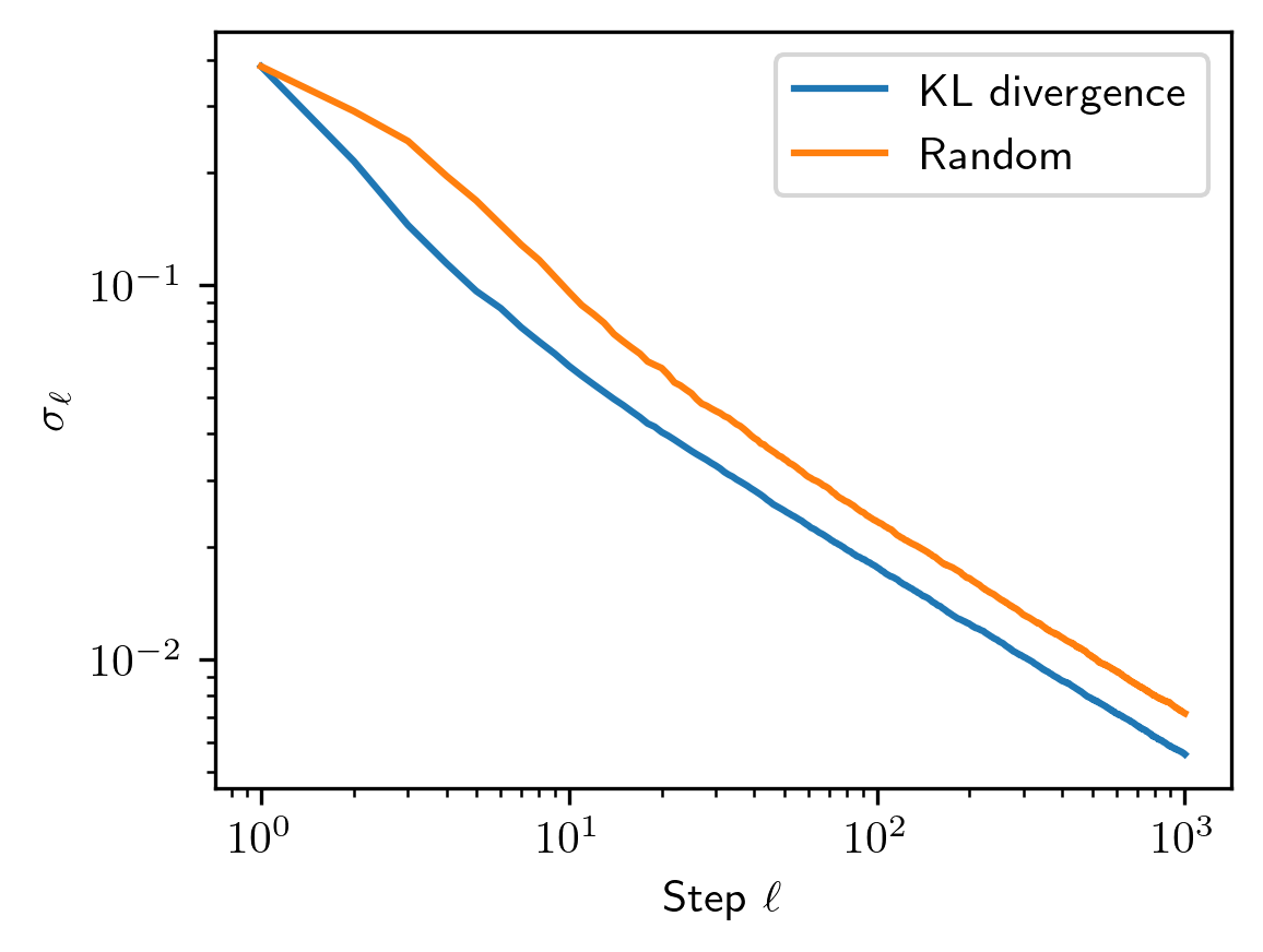
Figure 11: Standard deviation of the posterior $\sigma_{\ell}$ at each Bayesian step for the dephasing rate $\gamma$ in Markovian dephasing. The blue line represents the standard Bayesian approach in which at each step we find the optimal time using Eq. (37). The orange line simply chooses a random time $t_{\ell}\in\left[0.1,3\right]$. In both cases we start from the same uniformly distributed prior $U(\gamma_{\star}/3,3\gamma_{\star})$. At the beginning, the standard approach obtains an advantage, later on, once the number of measurements is sufficiently large, both instances become straight lines with slope $-\frac{1}{2}$ in this log-log plot. A total of 30 Bayesian runs were done in each case to estimate the expected $\sigma_{\ell}$. 50 measurement shots were taken at each step.

Appendix C Comparison to uniform-time Ramsey estimation

As discussed at the end of Sec. III.3.2, one can also compare the efficiency of the estimators introduced in the main text with a different one in which the measurement times are uniformly distributed over the whole time interval $T$. Such time distributions have been considered in previous works for Lindblad quantum tomography [87] and spin-locking spectroscopy of correlated noise [114]. In this appendix, we explore them in the context of the non-Markovian quantum dephasing.

This comparison can be done by calculating the determinants of the covariance matrix of the estimators, as is shown in Fig. 12 for two examples with different microscopic parameters. One parameter set shows a Markovian evolution, while the other leads to a non-Markovian one. The frequentist estimator with three optimal times is depicted by solid lines, and is always the best one in the asymptotic limit of an infinitely-large number of measurements $N_{\rm shot}\gg 1$. However, before reaching this regime, the uniform estimator displayed by dashed lines can become better. We are specially interested in the region with $10^{4}<N_{\rm shot}<10^{5}$, where the variance is already good enough to stop making more measurements, but the cost in terms of number of measurements is still not too big. In this region and for the Markovian case (blue), the uniform estimator is better than the frequentist one, which only considers three evolution times, set at the optimal values of the asymptotic limit. For the non-Markovian case (orange), the comparison is the opposite.

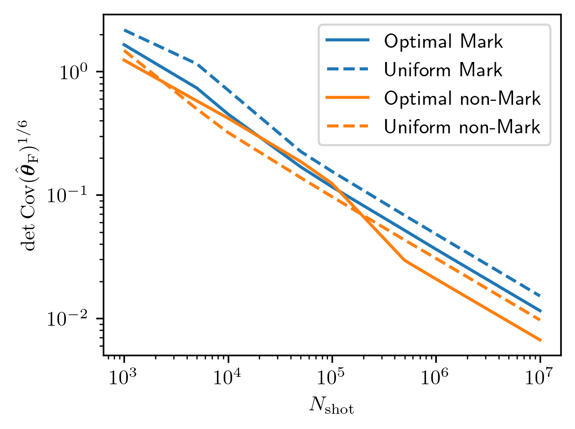
Figure 12: The efficiency of the optimal (solid) and uniform (dashed) estimators displayed in terms of $\det\mathrm{Cov}(\bm{\hat{\theta}}_{\rm F})^{1/6}$, with parameters $\bm{\theta}=(g^{2}_{\bar{n}},\kappa,\Delta_{\rm c})$ for different number of total measurements $N_{\rm shot}$. We consider two cases: (i) the Markovian case (blue) in which $\tau_{\rm c\star}=2/\kappa=0.3T_{2\star}$, $\Delta_{\rm c\star}=5/T_{2\star}$, (ii) the non-Markovian case (orange) where $\tau=2/\kappa=0.9T_{2\star}$, $\Delta_{\rm c}=5/T_{2\star}$. $T_{2}$ is set to 1, which makes $g^{2}\bar{n}\approx 2.7$ for the first and $g^{2}\bar{n}\approx 5.9$ for the second case. The uniform estimator measures time in 20 different equidistant points in the interval $t\in[0.02,3]$. Asymptotically $\det\mathrm{Cov}(\bm{\hat{\theta}}_{\rm F})^{1/6}$ scales as $1/\sqrt{N_{\rm shot}}$ for both estimators. For each value $N_{\rm shot}$, data is sampled and fitted to obtain an estimation. This is done a total of 5000 times to obtain afterwards the expected value of the covariance at that point. Bounds for the least squares algorithm were set to $(\bm{\theta}_{\!\star}/3,3\bm{\theta}_{\!\star})$. The initial guess was randomly chosen in that range.

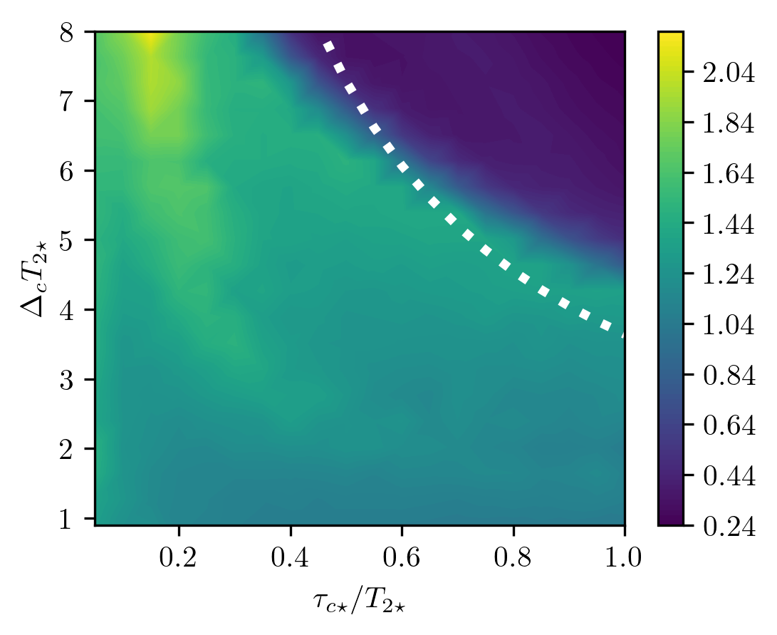
(a)

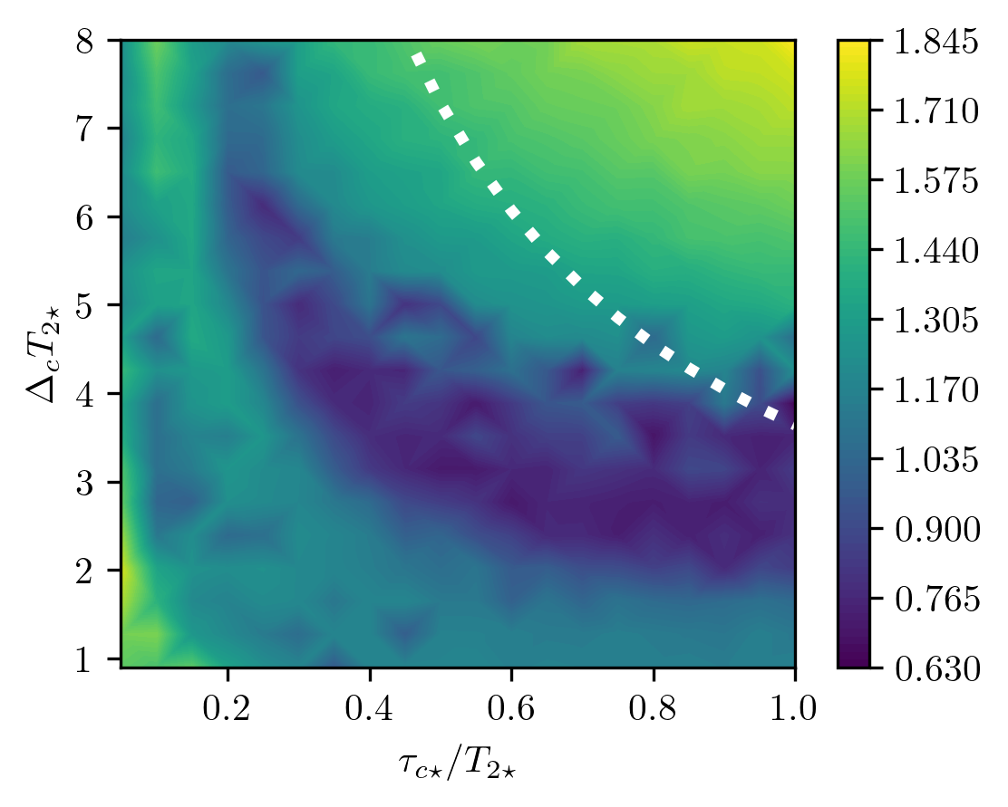
(b)

Figure 13: Ratios between determinants of covariance matrices of different estimators for different parameter values $\bm{\theta}_{\!\star}=(g^{2}_{\bar{n}\star},\kappa_{\star},\Delta_{\rm c\star})$ and a fixed number of total measurements $N=2\cdot 10^{4}$. $T_{2}=1$ for all combinations of $\tau$ and $\Delta_{\rm c}$. (a) The ratio between the uniform and the optimal estimator $r_{\mathrm{uni,opt}}=(\det\mathrm{Cov}(\bm{\hat{\theta}}_{\rm F,uni})/\det\mathrm{Cov}(\bm{\hat{\theta}}_{\rm F,opt}))^{1/6}$. (b) Ratio between the uniform estimator and the Bayesian approach, $r_{\mathrm{uni,Bay}}=(\det\mathrm{Cov}(\bm{\hat{\theta}}_{\rm F,uni})/\det\Sigma_{\ell_{\max}})^{1/6}$. For the frequentist estimators the same settings as in Fig. 12 were used to determine the expected value of the determinant. For the Bayesian approach a total of 30 experiments were run, with starting prior given by the continuous uniform distribution $U(\bm{\theta}_{\!\star}/3,3\bm{\theta}_{\!\star})$, i.e., the same bounds that were given to the least squares algorithm. The dashed white line separates the Markovian from the non-Markovian regime.

In order to extend this comparison between the uniform and the optimal-time estimators for a broader set of parameters, we compute the ratios between the determinant of the covariance matrix of the two estimators, $r_{\mathrm{uni,opt}}=\det\mathrm{Cov}(\bm{\hat{\theta}}_{\rm F,uni})^{1/6}/\det\mathrm{Cov}(\bm{\hat{\theta}}_{\rm F,opt})^{1/6}$, for different values of parameters $\tau_{\rm c\star}$ and $\Delta_{\rm c\star}$, as shown in Fig. 13a and analogously to what we do in Fig. 10 of Sec. III.3.2. This determinant ratios are computed for $N_{\rm shot}=2\cdot 10^{4}$, before reaching the region with asymptotic behavior, where the optimal estimator is always better than the uniform one. We can clearly see that the uniform estimator outperforms the optimal one in the Markovian regime (upper right region), while the opposite happens in the non-Markovian regime. While the optimal estimator is not realistic, since we need to know beforehand the true value of the parameters so that we can determine the optimal times, we may use it as a baseline to compare against other estimators or try to approximate it if we have some prior knowledge of the parameters. This comparison shows that the uniform estimator might be a good choice in the non-Markovian regime when doing a small number of shots.

In Fig. 13b we compare the uniform estimator with the Bayesian estimation. We can see that the Bayesian approach is better than the uniform estimator except for a small region in the Markovian regime.

Appendix D Error analysis and asymptotic statistics

We show here the asymptotic normality of the maximum-likelihood estimator (27) when $N_{\rm shot}$ tends to infinity and how this is related to the Fisher information in Eq. (31). The asymptotic covariance matrix is used in the main text to obtain the optimal times of the frequentist estimator and can be used to obtain approximate confidence intervals of estimations.

Our estimation $\bm{\hat{\theta}}_{F}$ is affected by the limited number of measurement shots $N_{i}$ at each point in time $t_{i}$, which will cause $\tilde{f}_{i}$ to behave as a normal random variable and will produce a random error in the final estimation of the parameters. The maximum-likelihood cost function reads

$$\mathsf{C}^{\rm pd}_{\mathrm{TL}}(\bm{\theta})=-\sum_{i,m_{x}}N_{i}\tilde{f}_{i,m_{x}}\log p_{i}(m_{x}|\bm{\theta}),$$ (69)

where $\tilde{f}_{i,m_{x}}$ denotes $\tilde{f}_{i}(m_{x}\,|\bm{\theta}_{\star})$ and $p_{i}(m_{x}|\bm{\theta})$ denotes $p^{\rm TL}_{i}(m_{x}|\bm{\theta})$. The minimum of the cost function satisfies

$$\partial_{\bm{\theta}}C_{\rm TL}^{\rm pd}=-\sum_{i,m_{x}}N_{i}\tilde{f}_{i,m_{x}}\frac{\partial_{\bm{\theta}}p_{i}(m_{x}|\bm{\theta})}{p_{i}(m_{x}|\bm{\theta})}=0.$$ (70)

Since $\tilde{f}_{i,m_{x}}=p_{i}(m_{x}|\bm{\theta}_{\star})+\Delta\tilde{f}_{i,m_{x}}$, with $\Delta\tilde{f}_{i,m_{x}}$ small, the minimum of the cost function is slightly displaced from the true minimum $\bm{\theta}_{\star}$ to $\bm{\theta}_{\star}+\Delta\bm{\theta}$. Taylor expanding Eq. (70) around $\bm{\theta}_{\star}$ to first order we have

$$\partial_{\theta_{j}}C_{\rm TL}^{\rm pd}\approx -\sum_{i,m_{x}}N_{i}\left[p_{i}(m_{x}|\bm{\theta})+\Delta\tilde{f}_{i,m_{x}}\right]\left[\left.\frac{\partial_{\theta_{j}}p_{i}(m_{x}|\bm{\theta})}{p_{i}(m_{x}|\bm{\theta})}\right|_{\bm{\theta}=\bm{\theta}_{\star}}\right.$$

$$\left.+\sum_{k}\left.\partial_{\theta_{k}}\frac{\partial_{\theta_{j}}p_{i}(m_{x}|\bm{\theta})}{p_{i}(m_{x}|\bm{\theta})}\right|_{\bm{\theta}=\bm{\theta}_{\star}}\Delta\theta_{k}\right]=0.$$ (71)

Keeping only first-order terms in $\Delta\bm{\theta}$ and $\Delta\tilde{f}_{i,m_{x}}$ and simplifying we obtain

$$\sum_{i,j}\Delta\bm{\theta}_{j}N_{i}[I_{i}(\bm{\theta}_{\star})]_{jk}=\sum_{i,m_{x}}N_{i}\Delta\tilde{f}_{i,m_{x}}\left.\frac{\partial_{\theta_{k}}p_{i}(m_{x}|\bm{\theta})}{p_{i}(m_{x}|\bm{\theta})}\right|_{\bm{\theta}=\bm{\theta}_{\star}},$$ (72)

where we have defined the matrix

$$[I_{i} (\bm{\theta}_{\star})]_{jk}=$$ (73)

$$\sum_{m_{x}}p_{i}(m_{x}|\bm{\theta}_{\star})\partial_{\theta_{j}}\log p_{i}(m_{x}|\bm{\theta})\partial_{\theta_{k}}\log p_{i}(m_{x}|\bm{\theta})|_{\bm{\theta}=\bm{\theta}_{\star}}.$$

Note that this is the Fisher information given in Eq. (30). Taking into account that $\Delta\tilde{f}_{i,1}=-\Delta\tilde{f}_{i,0}$ and $\tilde{f}_{i,1}=1-\tilde{f}_{i,0}$, and defining the matrices

$$J_{jk}=\sum_{i}N_{i}[I_{i}(\bm{\theta}_{\star})]_{jk},\quad\ F_{ji}=N_{i}\frac{\left.\partial_{\theta_{j}}p_{i}(0|\bm{\theta})\right|_{\bm{\theta}=\bm{\theta}_{\star}}}{p_{i}(0|\bm{\theta}_{\star})(1-p_{i}(0|\bm{\theta}_{\star}))},$$ (74)

we arrive at the expression

$$\Delta\theta_{k}=\sum_{i,j}J^{-1}_{jk}F_{ji}\Delta\tilde{f}_{i,0},$$ (75)

which relates differences between the expected and measured values $\Delta\tilde{f}_{i,m_{x}}=\tilde{f}_{i,m_{x}}-p_{i}(m_{x}|\bm{\theta}_{\star})$ to differences between the estimated and the true parameters $\Delta\theta_{k}$. When $N_{i}$ is sufficiently large, $\tilde{f}_{i,0}$ behaves as the normal distribution $N\left[\mu=p_{i}(0|\bm{\theta}_{\star}),\sigma_{f}^{2}=p_{i}(0|\bm{\theta}_{\star})p_{i}(1|\bm{\theta}_{\star})/N_{i}\right]$. Thus, we have

$$\Delta\tilde{f}_{i,0}\sim N\left[\mu=0,\sigma^{2}_{f_{i}}=p_{i}(0|\bm{\theta}_{\star})p_{i}(1|\bm{\theta}_{\star})/N_{i}\right].$$ (76)

After the linear transformation (75), we obtain that $\Delta\bm{\theta}$ behaves as

$$\Delta\bm{\theta}\sim N\left[\mu=0,\ \Sigma_{\hat{\bm{\theta}}}=J^{-1}\right],$$ (77)

where we have used that $J^{-1}F\mathrm{diag}(\sigma^{2}_{f})F^{T}(J^{-1})^{T}=J^{-1}$. Thus, the shot noise produces a normal random error with covariance matrix $\Sigma_{\bm{\theta}}=J^{-1}$ which scales as $1/N_{\rm shot}$, with $N_{\rm shot}=\sum_{i}N_{i}$, which is the result presented in Eq. (31).

References

- Nielsen and Chuang [2010] M. A. Nielsen and I. L. Chuang, Quantum Computation and Quantum Information: 10th Anniversary Edition (Cambridge University Press, 2010).
- Bruzewicz et al. [2019] C. D. Bruzewicz, J. Chiaverini, R. McConnell, and J. M. Sage, Trapped-ion quantum computing: Progress and challenges, Applied Physics Reviews 6, 021314 (2019).
- Morgado and Whitlock [2021] M. Morgado and S. Whitlock, Quantum simulation and computing with Rydberg-interacting qubits, AVS Quantum Science 3, 023501 (2021).
- Wendin [2017] G. Wendin, Quantum information processing with superconducting circuits: a review, Reports on Progress in Physics 80, 106001 (2017).
- Arute et al. [2019] F. Arute, K. Arya, R. Babbush, D. Bacon, J. C. Bardin, R. Barends, R. Biswas, S. Boixo, F. G. S. L. Brandao, D. A. Buell, B. Burkett, Y. Chen, Z. Chen, B. Chiaro, R. Collins, W. Courtney, A. Dunsworth, E. Farhi, B. Foxen, A. Fowler, C. Gidney, M. Giustina, R. Graff, K. Guerin, S. Habegger, M. P. Harrigan, M. J. Hartmann, A. Ho, M. Hoffmann, T. Huang, T. S. Humble, S. V. Isakov, E. Jeffrey, Z. Jiang, D. Kafri, K. Kechedzhi, J. Kelly, P. V. Klimov, S. Knysh, A. Korotkov, F. Kostritsa, D. Landhuis, M. Lindmark, E. Lucero, D. Lyakh, S. Mandrà, J. R. McClean, M. McEwen, A. Megrant, X. Mi, K. Michielsen, M. Mohseni, J. Mutus, O. Naaman, M. Neeley, C. Neill, M. Y. Niu, E. Ostby, A. Petukhov, J. C. Platt, C. Quintana, E. G. Rieffel, P. Roushan, N. C. Rubin, D. Sank, K. J. Satzinger, V. Smelyanskiy, K. J. Sung, M. D. Trevithick, A. Vainsencher, B. Villalonga, T. White, Z. J. Yao, P. Yeh, A. Zalcman, H. Neven, and J. M. Martinis, Quantum supremacy using a programmable superconducting processor, Nature 574, 505 (2019).
- Zhong et al. [2020] H.-S. Zhong, H. Wang, Y.-H. Deng, M.-C. Chen, L.-C. Peng, Y.-H. Luo, J. Qin, D. Wu, X. Ding, Y. Hu, P. Hu, X.-Y. Yang, W.-J. Zhang, H. Li, Y. Li, X. Jiang, L. Gan, G. Yang, L. You, Z. Wang, L. Li, N.-L. Liu, C.-Y. Lu, and J.-W. Pan, Quantum computational advantage using photons, Science 370, 1460 (2020).
- Pino et al. [2021] J. M. Pino, J. M. Dreiling, C. Figgatt, J. P. Gaebler, S. A. Moses, M. S. Allman, C. H. Baldwin, M. Foss-Feig, D. Hayes, K. Mayer, C. Ryan-Anderson, and B. Neyenhuis, Demonstration of the trapped-ion quantum CCD computer architecture, Nature 592, 209 (2021).
- Egan et al. [2021] L. Egan, D. M. Debroy, C. Noel, A. Risinger, D. Zhu, D. Biswas, M. Newman, M. Li, K. R. Brown, M. Cetina, and C. Monroe, Fault-tolerant control of an error-corrected qubit, Nature 598, 281 (2021).
- Postler et al. [2022] L. Postler, S. Heuen, I. Pogorelov, M. Rispler, T. Feldker, M. Meth, C. D. Marciniak, R. Stricker, M. Ringbauer, R. Blatt, P. Schindler, M. Müller, and T. Monz, Demonstration of fault-tolerant universal quantum gate operations, Nature 605, 675 (2022).
- Krinner et al. [2022] S. Krinner, N. Lacroix, A. Remm, A. Di Paolo, E. Genois, C. Leroux, C. Hellings, S. Lazar, F. Swiadek, J. Herrmann, G. J. Norris, C. K. Andersen, M. Müller, A. Blais, C. Eichler, and A. Wallraff, Realizing repeated quantum error correction in a distance-three surface code, Nature 605, 669 (2022).
- Zhao et al. [2022] Y. Zhao, Y. Ye, H.-L. Huang, Y. Zhang, D. Wu, H. Guan, Q. Zhu, Z. Wei, T. He, S. Cao, F. Chen, T.-H. Chung, H. Deng, D. Fan, M. Gong, C. Guo, S. Guo, L. Han, N. Li, S. Li, Y. Li, F. Liang, J. Lin, H. Qian, H. Rong, H. Su, L. Sun, S. Wang, Y. Wu, Y. Xu, C. Ying, J. Yu, C. Zha, K. Zhang, Y.-H. Huo, C.-Y. Lu, C.-Z. Peng, X. Zhu, and J.-W. Pan, Realization of an error-correcting surface code with superconducting qubits, Phys. Rev. Lett. 129, 030501 (2022).
- Acharya et al. [2023] R. Acharya, I. Aleiner, R. Allen, T. I. Andersen, M. Ansmann, F. Arute, K. Arya, A. Asfaw, J. Atalaya, R. Babbush, D. Bacon, J. C. Bardin, J. Basso, A. Bengtsson, S. Boixo, G. Bortoli, A. Bourassa, J. Bovaird, L. Brill, M. Broughton, B. B. Buckley, D. A. Buell, T. Burger, B. Burkett, N. Bushnell, Y. Chen, Z. Chen, B. Chiaro, J. Cogan, R. Collins, P. Conner, W. Courtney, A. L. Crook, B. Curtin, D. M. Debroy, A. Del Toro Barba, S. Demura, A. Dunsworth, D. Eppens, C. Erickson, L. Faoro, E. Farhi, R. Fatemi, L. Flores Burgos, E. Forati, A. G. Fowler, B. Foxen, W. Giang, C. Gidney, D. Gilboa, M. Giustina, A. Grajales Dau, J. A. Gross, S. Habegger, M. C. Hamilton, M. P. Harrigan, S. D. Harrington, O. Higgott, J. Hilton, M. Hoffmann, S. Hong, T. Huang, A. Huff, W. J. Huggins, L. B. Ioffe, S. V. Isakov, J. Iveland, E. Jeffrey, Z. Jiang, C. Jones, P. Juhas, D. Kafri, K. Kechedzhi, J. Kelly, T. Khattar, M. Khezri, M. Kieferová, S. Kim, A. Kitaev, P. V. Klimov, A. R. Klots, A. N. Korotkov, F. Kostritsa, J. M. Kreikebaum, D. Landhuis, P. Laptev, K.-M. Lau, L. Laws, J. Lee, K. Lee, B. J. Lester, A. Lill, W. Liu, A. Locharla, E. Lucero, F. D. Malone, J. Marshall, O. Martin, J. R. McClean, T. McCourt, M. McEwen, A. Megrant, B. Meurer Costa, X. Mi, K. C. Miao, M. Mohseni, S. Montazeri, A. Morvan, E. Mount, W. Mruczkiewicz, O. Naaman, M. Neeley, C. Neill, A. Nersisyan, H. Neven, M. Newman, J. H. Ng, A. Nguyen, M. Nguyen, M. Y. Niu, T. E. O’Brien, A. Opremcak, J. Platt, A. Petukhov, R. Potter, L. P. Pryadko, C. Quintana, P. Roushan, N. C. Rubin, N. Saei, D. Sank, K. Sankaragomathi, K. J. Satzinger, H. F. Schurkus, C. Schuster, M. J. Shearn, A. Shorter, V. Shvarts, J. Skruzny, V. Smelyanskiy, W. C. Smith, G. Sterling, D. Strain, M. Szalay, A. Torres, G. Vidal, B. Villalonga, C. Vollgraff Heidweiller, T. White, C. Xing, Z. J. Yao, P. Yeh, J. Yoo, G. Young, A. Zalcman, Y. Zhang, N. Zhu, and G. Q. AI, Suppressing quantum errors by scaling a surface code logical qubit, Nature 614, 676 (2023).
- Kim et al. [2023] Y. Kim, A. Eddins, S. Anand, K. X. Wei, E. van den Berg, S. Rosenblatt, H. Nayfeh, Y. Wu, M. Zaletel, K. Temme, and A. Kandala, Evidence for the utility of quantum computing before fault tolerance, Nature 618, 500 (2023).
- Bluvstein et al. [2024] D. Bluvstein, S. J. Evered, A. A. Geim, S. H. Li, H. Zhou, T. Manovitz, S. Ebadi, M. Cain, M. Kalinowski, D. Hangleiter, J. P. Bonilla Ataides, N. Maskara, I. Cong, X. Gao, P. Sales Rodriguez, T. Karolyshyn, G. Semeghini, M. J. Gullans, M. Greiner, V. Vuletić, and M. D. Lukin, Logical quantum processor based on reconfigurable atom arrays, Nature 626, 58 (2024).
- Gupta et al. [2024] R. S. Gupta, N. Sundaresan, T. Alexander, C. J. Wood, S. T. Merkel, M. B. Healy, M. Hillenbrand, T. Jochym-O’Connor, J. R. Wootton, T. J. Yoder, A. W. Cross, M. Takita, and B. J. Brown, Encoding a magic state with beyond break-even fidelity, Nature 625, 259 (2024).
- Wang et al. [2023] Y. Wang, S. Simsek, T. M. Gatterman, J. A. Gerber, K. Gilmore, D. Gresh, N. Hewitt, C. V. Horst, M. Matheny, T. Mengle, B. Neyenhuis, and B. Criger, Fault-tolerant one-bit addition with the smallest interesting colour code (2023), arXiv:2309.09893 [quant-ph] .
- Yamamoto et al. [2024] K. Yamamoto, S. Duffield, Y. Kikuchi, and D. Muñoz Ramo, Demonstrating Bayesian quantum phase estimation with quantum error detection, Physical Review Research 6, 10.1103/physrevresearch.6.013221 (2024).
- Ryan-Anderson et al. [2022] C. Ryan-Anderson, N. C. Brown, M. S. Allman, B. Arkin, G. Asa-Attuah, C. Baldwin, J. Berg, J. G. Bohnet, S. Braxton, N. Burdick, J. P. Campora, A. Chernoguzov, J. Esposito, B. Evans, D. Francois, J. P. Gaebler, T. M. Gatterman, J. Gerber, K. Gilmore, D. Gresh, A. Hall, A. Hankin, J. Hostetter, D. Lucchetti, K. Mayer, J. Myers, B. Neyenhuis, J. Santiago, J. Sedlacek, T. Skripka, A. Slattery, R. P. Stutz, J. Tait, R. Tobey, G. Vittorini, J. Walker, and D. Hayes, Implementing fault-tolerant entangling gates on the five-qubit code and the color code (2022).
- Dalzell et al. [2023] A. M. Dalzell, S. McArdle, M. Berta, P. Bienias, C.-F. Chen, A. Gilyén, C. T. Hann, M. J. Kastoryano, E. T. Khabiboulline, A. Kubica, G. Salton, S. Wang, and F. G. S. L. Brandão, Quantum algorithms: A survey of applications and end-to-end complexities (2023), arXiv:2310.03011 [quant-ph] .
- Viola et al. [1999] L. Viola, E. Knill, and S. Lloyd, Dynamical decoupling of open quantum systems, Phys. Rev. Lett. 82, 2417 (1999).
- Khodjasteh and Lidar [2005] K. Khodjasteh and D. A. Lidar, Fault-tolerant quantum dynamical decoupling, Phys. Rev. Lett. 95, 180501 (2005).
- Khodjasteh and Viola [2009] K. Khodjasteh and L. Viola, Dynamically error-corrected gates for universal quantum computation, Phys. Rev. Lett. 102, 080501 (2009).
- Lidar [2014] D. A. Lidar, Review of decoherence-free subspaces, noiseless subsystems, and dynamical decoupling, in Quantum Information and Computation for Chemistry (John Wiley & Sons, Ltd, 2014) pp. 295–354.
- Temme et al. [2017] K. Temme, S. Bravyi, and J. M. Gambetta, Error mitigation for short-depth quantum circuits, Phys. Rev. Lett. 119, 180509 (2017).
- Nation et al. [2021] P. D. Nation, H. Kang, N. Sundaresan, and J. M. Gambetta, Scalable mitigation of measurement errors on quantum computers, PRX Quantum 2, 040326 (2021).
- van den Berg et al. [2023] E. van den Berg, Z. K. Minev, A. Kandala, and K. Temme, Probabilistic error cancellation with sparse Pauli–Lindblad models on noisy quantum processors, Nature Physics 19, 1116 (2023).
- Cai et al. [2023] Z. Cai, R. Babbush, S. C. Benjamin, S. Endo, W. J. Huggins, Y. Li, J. R. McClean, and T. E. O’Brien, Quantum error mitigation, Rev. Mod. Phys. 95, 045005 (2023).
- Calderbank and Shor [1996] A. R. Calderbank and P. W. Shor, Good quantum error-correcting codes exist, Phys. Rev. A 54, 1098 (1996).
- Steane [1996] A. M. Steane, Error correcting codes in quantum theory, Phys. Rev. Lett. 77, 793 (1996).
- Terhal [2015] B. M. Terhal, Quantum error correction for quantum memories, Rev. Mod. Phys. 87, 307 (2015).
- Eisert et al. [2020] J. Eisert, D. Hangleiter, N. Walk, I. Roth, D. Markham, R. Parekh, U. Chabaud, and E. Kashefi, Quantum certification and benchmarking, Nature Reviews Physics 2, 382 (2020).
- Kliesch and Roth [2021] M. Kliesch and I. Roth, Theory of quantum system certification, PRX Quantum 2, 010201 (2021).
- Gebhart et al. [2023] V. Gebhart, R. Santagati, A. A. Gentile, E. M. Gauger, D. Craig, N. Ares, L. Banchi, F. Marquardt, L. Pezzè, and C. Bonato, Learning quantum systems, Nature Reviews Physics 5, 141 (2023).
- Zanardi and Rasetti [1997] P. Zanardi and M. Rasetti, Noiseless quantum codes, Phys. Rev. Lett. 79, 3306 (1997).
- Lidar et al. [1998] D. A. Lidar, I. L. Chuang, and K. B. Whaley, Decoherence-free subspaces for quantum computation, Phys. Rev. Lett. 81, 2594 (1998).
- Knill et al. [2000] E. Knill, R. Laflamme, and L. Viola, Theory of quantum error correction for general noise, Phys. Rev. Lett. 84, 2525 (2000).
- Kempe et al. [2001] J. Kempe, D. Bacon, D. A. Lidar, and K. B. Whaley, Theory of decoherence-free fault-tolerant universal quantum computation, Phys. Rev. A 63, 042307 (2001).
- Lidar and Birgitta Whaley [2003] D. A. Lidar and K. Birgitta Whaley, Decoherence-free subspaces and subsystems, in Lecture Notes in Physics (Springer Berlin Heidelberg, 2003) p. 83–120.
- Viola and Lloyd [1998] L. Viola and S. Lloyd, Dynamical suppression of decoherence in two-state quantum systems, Phys. Rev. A 58, 2733 (1998).
- Kofman and Kurizki [2004] A. G. Kofman and G. Kurizki, Unified theory of dynamically suppressed qubit decoherence in thermal baths, Phys. Rev. Lett. 93, 130406 (2004).
- Gordon et al. [2007] G. Gordon, N. Erez, and G. Kurizki, Universal dynamical decoherence control of noisy single- and multi-qubit systems, Journal of Physics B: Atomic, Molecular and Optical Physics 40, S75 (2007).
- Uhrig [2007] G. S. Uhrig, Keeping a quantum bit alive by optimized -pulse sequences, Phys. Rev. Lett. 98, 100504 (2007).
- Cywiński et al. [2008] L. Cywiński, R. M. Lutchyn, C. P. Nave, and S. Das Sarma, How to enhance dephasing time in superconducting qubits, Phys. Rev. B 77, 174509 (2008).
- Biercuk et al. [2011] M. J. Biercuk, A. C. Doherty, and H. Uys, Dynamical decoupling sequence construction as a filter-design problem, Journal of Physics B: Atomic, Molecular and Optical Physics 44, 154002 (2011).
- Clemens et al. [2004] J. P. Clemens, S. Siddiqui, and J. Gea-Banacloche, Quantum error correction against correlated noise, Phys. Rev. A 69, 062313 (2004).
- Klesse and Frank [2005] R. Klesse and S. Frank, Quantum error correction in spatially correlated quantum noise, Phys. Rev. Lett. 95, 230503 (2005).
- Aharonov et al. [2006] D. Aharonov, A. Kitaev, and J. Preskill, Fault-tolerant quantum computation with long-range correlated noise, Phys. Rev. Lett. 96, 050504 (2006).
- Terhal and Burkard [2005] B. M. Terhal and G. Burkard, Fault-tolerant quantum computation for local non-Markovian noise, Phys. Rev. A 71, 012336 (2005).
- Aliferis et al. [2006] P. Aliferis, D. Gottesman, and J. Preskill, Quantum accuracy threshold for concatenated distance-3 codes, Quantum Info. Comput. 6, 97–165 (2006).
- Ng and Preskill [2009] H. K. Ng and J. Preskill, Fault-tolerant quantum computation versus Gaussian noise, Phys. Rev. A 79, 032318 (2009).
- Ángel Rivas et al. [2014] Ángel Rivas, S. F. Huelga, and M. B. Plenio, Quantum non-Markovianity: characterization, quantification and detection, Reports on Progress in Physics 77, 094001 (2014).
- Breuer et al. [2016] H.-P. Breuer, E.-M. Laine, J. Piilo, and B. Vacchini, Colloquium: Non-Markovian dynamics in open quantum systems, Rev. Mod. Phys. 88, 021002 (2016).
- Li et al. [2018] L. Li, M. J. Hall, and H. M. Wiseman, Concepts of quantum non-Markovianity: A hierarchy, Physics Reports 759, 1–51 (2018).
- Addis et al. [2015] C. Addis, F. Ciccarello, M. Cascio, G. M. Palma, and S. Maniscalco, Dynamical decoupling efficiency versus quantum non-Markovianity, New Journal of Physics 17, 123004 (2015).
- Berk et al. [2023] G. D. Berk, S. Milz, F. A. Pollock, and K. Modi, Extracting quantum dynamical resources: consumption of non-Markovianity for noise reduction, npj Quantum Information 9, 104 (2023).
- Hakoshima et al. [2021] H. Hakoshima, Y. Matsuzaki, and S. Endo, Relationship between costs for quantum error mitigation and non-Markovian measures, Phys. Rev. A 103, 012611 (2021).
- Donvil et al. [2023] B. I. C. Donvil, R. Lechler, J. Ankerhold, and P. Muratore-Ginanneschi, Quantum trajectory approach to error mitigation (2023), arXiv:2305.19874 [quant-ph] .
- Chuang and Nielsen [1997] I. L. Chuang and M. A. Nielsen, Prescription for experimental determination of the dynamics of a quantum black box, Journal of Modern Optics 44, 2455 (1997).
- Poyatos et al. [1997] J. F. Poyatos, J. I. Cirac, and P. Zoller, Complete characterization of a quantum process: The two-bit quantum gate, Phys. Rev. Lett. 78, 390 (1997).
- Fiurášek and Hradil [2001] J. Fiurášek and Z. c. v. Hradil, Maximum-likelihood estimation of quantum processes, Phys. Rev. A 63, 020101 (2001).
- Sacchi [2001] M. F. Sacchi, Maximum-likelihood reconstruction of completely positive maps, Phys. Rev. A 63, 054104 (2001).
- Ježek et al. [2003] M. Ježek, J. Fiurášek, and Z. c. v. Hradil, Quantum inference of states and processes, Phys. Rev. A 68, 012305 (2003).
- Nielsen and Chuang [2000] M. A. Nielsen and I. L. Chuang, Quantum Computation and Quantum Information (Cambridge University Press, 2000).
- Watrous [2018] J. Watrous, The Theory of Quantum Information (Cambridge University Press, 2018).
- Childs et al. [2001] A. M. Childs, I. L. Chuang, and D. W. Leung, Realization of quantum process tomography in NMR, Phys. Rev. A 64, 012314 (2001).
- Weinstein et al. [2004] Y. S. Weinstein, T. F. Havel, J. Emerson, N. Boulant, M. Saraceno, S. Lloyd, and D. G. Cory, Quantum process tomography of the quantum Fourier transform, The Journal of Chemical Physics 121, 6117 (2004).
- Mitchell et al. [2003] M. W. Mitchell, C. W. Ellenor, S. Schneider, and A. M. Steinberg, Diagnosis, prescription, and prognosis of a Bell-state filter by quantum process tomography, Phys. Rev. Lett. 91, 120402 (2003).
- O’Brien et al. [2004] J. L. O’Brien, G. J. Pryde, A. Gilchrist, D. F. V. James, N. K. Langford, T. C. Ralph, and A. G. White, Quantum process tomography of a controlled-not gate, Phys. Rev. Lett. 93, 080502 (2004).
- Riebe et al. [2006] M. Riebe, K. Kim, P. Schindler, T. Monz, P. O. Schmidt, T. K. Körber, W. Hänsel, H. Häffner, C. F. Roos, and R. Blatt, Process tomography of ion trap quantum gates, Phys. Rev. Lett. 97, 220407 (2006).
- Home et al. [2009] J. P. Home, D. Hanneke, J. D. Jost, J. M. Amini, D. Leibfried, and D. J. Wineland, Complete methods set for scalable ion trap quantum information processing, Science 325, 1227 (2009).
- Monz et al. [2009] T. Monz, K. Kim, W. Hänsel, M. Riebe, A. S. Villar, P. Schindler, M. Chwalla, M. Hennrich, and R. Blatt, Realization of the quantum Toffoli gate with trapped ions, Phys. Rev. Lett. 102, 040501 (2009).
- Bialczak et al. [2010] R. C. Bialczak, M. Ansmann, M. Hofheinz, E. Lucero, M. Neeley, A. D. O’Connell, D. Sank, H. Wang, J. Wenner, M. Steffen, A. N. Cleland, and J. M. Martinis, Quantum process tomography of a universal entangling gate implemented with Josephson phase qubits, Nature Physics 6, 409 (2010).
- Poletto et al. [2012] S. Poletto, J. M. Gambetta, S. T. Merkel, J. A. Smolin, J. M. Chow, A. D. Córcoles, G. A. Keefe, M. B. Rothwell, J. R. Rozen, D. W. Abraham, C. Rigetti, and M. Steffen, Entanglement of two superconducting qubits in a waveguide cavity via monochromatic two-photon excitation, Phys. Rev. Lett. 109, 240505 (2012).
- Breuer and Petruccione [2002a] H. P. Breuer and F. Petruccione, The theory of open quantum systems (Oxford University Press, Great Clarendon Street, 2002).
- de Vega and Alonso [2017] I. de Vega and D. Alonso, Dynamics of non-Markovian open quantum systems, Rev. Mod. Phys. 89, 015001 (2017).
- Chruściński [2022] D. Chruściński, Dynamical maps beyond Markovian regime (2022), arXiv:2209.14902 [quant-ph] .
- Velázquez et al. [2024] J. M. S. Velázquez, A. Steiner, R. Freund, M. Guevara-Bertsch, C. D. Marciniak, T. Monz, and A. Bermudez, Dynamical quantum maps for single-qubit gates under non-Markovian phase noise (2024), arXiv:2402.14530 [quant-ph] .
- Lindblad [1976] G. Lindblad, On the generators of quantum dynamical semigroups, Communications in Mathematical Physics 48, 119 (1976).
- Gorini et al. [1976] V. Gorini, A. Kossakowski, and E. C. G. Sudarshan, Completely positive dynamical semigroups of n‐level systems, Journal of Mathematical Physics 17, 821 (1976).
- Wolf et al. [2008] M. M. Wolf, J. Eisert, T. S. Cubitt, and J. I. Cirac, Assessing non-Markovian quantum dynamics, Physical Review Letters 101, 10.1103/physrevlett.101.150402 (2008).
- Boulant et al. [2003] N. Boulant, T. F. Havel, M. A. Pravia, and D. G. Cory, Robust method for estimating the Lindblad operators of a dissipative quantum process from measurements of the density operator at multiple time points, Phys. Rev. A 67, 042322 (2003).
- Howard et al. [2006] M. Howard, J. Twamley, C. Wittmann, T. Gaebel, F. Jelezko, and J. Wrachtrup, Quantum process tomography and Linblad estimation of a solid-state qubit, New Journal of Physics 8, 33 (2006).
- Onorati et al. [2021] E. Onorati, T. Kohler, and T. Cubitt, Fitting quantum noise models to tomography data (2021), arXiv:2103.17243 [quant-ph] .
- Bairey et al. [2020] E. Bairey, C. Guo, D. Poletti, N. H. Lindner, and I. Arad, Learning the dynamics of open quantum systems from their steady states, New Journal of Physics 22, 032001 (2020).
- Pastori et al. [2022] L. Pastori, T. Olsacher, C. Kokail, and P. Zoller, Characterization and verification of Trotterized digital quantum simulation via Hamiltonian and Liouvillian learning, PRX Quantum 3, 030324 (2022).
- França et al. [2022] D. S. França, L. A. Markovich, V. V. Dobrovitski, A. H. Werner, and J. Borregaard, Efficient and robust estimation of many-qubit Hamiltonians (2022), arXiv:2205.09567 [quant-ph] .
- Samach et al. [2022] G. O. Samach, A. Greene, J. Borregaard, M. Christandl, J. Barreto, D. K. Kim, C. M. McNally, A. Melville, B. M. Niedzielski, Y. Sung, D. Rosenberg, M. E. Schwartz, J. L. Yoder, T. P. Orlando, J. I.-J. Wang, S. Gustavsson, M. Kjaergaard, and W. D. Oliver, Lindblad tomography of a superconducting quantum processor, Phys. Rev. Appl. 18, 064056 (2022).
- Zhang et al. [2022] H. Zhang, B. Pokharel, E. Levenson-Falk, and D. Lidar, Predicting non-Markovian superconducting-qubit dynamics from tomographic reconstruction, Phys. Rev. Appl. 17, 054018 (2022).
- Ben Av et al. [2020] E. Ben Av, Y. Shapira, N. Akerman, and R. Ozeri, Direct reconstruction of the quantum-master-equation dynamics of a trapped-ion qubit, Phys. Rev. A 101, 062305 (2020).
- Dobrynin et al. [2024] D. Dobrynin, L. Cardarelli, M. Müller, and A. Bermudez, Compressed-sensing Lindbladian quantum tomography with trapped ions (2024), arXiv:2403.07462 [quant-ph] .
- Chaturvedi and Shibata [1979] S. Chaturvedi and F. Shibata, Time-convolutionless projection operator formalism for elimination of fast variables. Applications to Brownian motion, Zeitschrift für Physik B Condensed Matter 35, 297 (1979).
- Nakajima [1958] S. Nakajima, On Quantum Theory of Transport Phenomena: Steady Diffusion, Progress of Theoretical Physics 20, 948 (1958).
- Zwanzig [2004] R. Zwanzig, Ensemble Method in the Theory of Irreversibility, The Journal of Chemical Physics 33, 1338 (2004).
- Hall et al. [2014] M. J. W. Hall, J. D. Cresser, L. Li, and E. Andersson, Canonical form of master equations and characterization of non-Markovianity, Phys. Rev. A 89, 042120 (2014).
- Bužek [1998] V. Bužek, Reconstruction of Liouvillian superoperators, Phys. Rev. A 58, 1723 (1998).
- Rossi [2018] R. J. Rossi, Mathematical statistics an introduction to likelihood based inference, 1st ed. (John Wiley & Sons, Hoboken, NJ, 2018).
- Rivas et al. [2010] A. Rivas, S. F. Huelga, and M. B. Plenio, Entanglement and non-Markovianity of quantum evolutions, Phys. Rev. Lett. 105, 050403 (2010).
- Kofman and Kurizki [2000] A. G. Kofman and G. Kurizki, Acceleration of quantum decay processes by frequent observations, Nature 405, 546 (2000).
- Kofman and Kurizki [2001] A. G. Kofman and G. Kurizki, Universal dynamical control of quantum mechanical decay: Modulation of the coupling to the continuum, Phys. Rev. Lett. 87, 270405 (2001).
- Uhrig [2008] G. S. Uhrig, Exact results on dynamical decoupling by pulses in quantum information processes, New Journal of Physics 10, 083024 (2008).
- Almog et al. [2011] I. Almog, Y. Sagi, G. Gordon, G. Bensky, G. Kurizki, and N. Davidson, Direct measurement of the system–environment coupling as a tool for understanding decoherence and dynamical decoupling, Journal of Physics B: Atomic, Molecular and Optical Physics 44, 154006 (2011).
- Rivas et al. [2014] Á. Rivas, S. F. Huelga, and M. B. Plenio, Quantum non-Markovianity: Characterization, quantification and detection, Reports on Progress in Physics 77, 094001 (2014).
- Kullback and Leibler [1951] S. Kullback and R. A. Leibler, On information and sufficiency, The Annals of Mathematical Statistics 22, 79 (1951).
- Mogilevtsev et al. [2012] D. Mogilevtsev, J. Řeháček, and Z. Hradil, Self-calibration for self-consistent tomography, New Journal of Physics 14, 095001 (2012).
- James [2006] F. James, Statistical Methods in Experimental Physics, 2nd ed. (WORLD SCIENTIFIC, 2006) https://www.worldscientific.com/doi/pdf/10.1142/6096 .
- Hoadley [1971] B. Hoadley, Asymptotic Properties of Maximum Likelihood Estimators for the Independent Not Identically Distributed Case, The Annals of Mathematical Statistics 42, 1977 (1971).
- Virtanen et al. [2020] P. Virtanen, R. Gommers, T. E. Oliphant, M. Haberland, T. Reddy, D. Cournapeau, E. Burovski, P. Peterson, W. Weckesser, J. Bright, S. J. van der Walt, M. Brett, J. Wilson, K. J. Millman, N. Mayorov, A. R. J. Nelson, E. Jones, R. Kern, E. Larson, C. J. Carey, İ. Polat, Y. Feng, E. W. Moore, J. VanderPlas, D. Laxalde, J. Perktold, R. Cimrman, I. Henriksen, E. A. Quintero, C. R. Harris, A. M. Archibald, A. H. Ribeiro, F. Pedregosa, P. van Mulbregt, and SciPy 1.0 Contributors, SciPy 1.0: Fundamental Algorithms for Scientific Computing in Python, Nature Methods 17, 261 (2020).
- Blume-Kohout [2012] R. Blume-Kohout, Robust error bars for quantum tomography (2012), arXiv:1202.5270 [quant-ph] .
- Thinh et al. [2019] L. P. Thinh, P. Faist, J. Helsen, D. Elkouss, and S. Wehner, Practical and reliable error bars for quantum process tomography, Phys. Rev. A 99, 052311 (2019).
- Granade et al. [2017] C. Granade, C. Ferrie, I. Hincks, S. Casagrande, T. Alexander, J. Gross, M. Kononenko, and Y. Sanders, QInfer: Statistical inference software for quantum applications, Quantum 1, 5 (2017).
- Gardiner [2004] C. W. Gardiner, Handbook of stochastic methods for physics, chemistry and the natural sciences, 3rd ed., Springer Series in Synergetics, Vol. 13 (Springer-Verlag, Berlin, 2004) pp. xviii+415.
- Gillespie [1996] D. T. Gillespie, The mathematics of Brownian motion and Johnson noise, American Journal of Physics 64, 225 (1996).
- Clerk et al. [2010] A. A. Clerk, M. H. Devoret, S. M. Girvin, F. Marquardt, and R. J. Schoelkopf, Introduction to quantum noise, measurement, and amplification, Rev. Mod. Phys. 82, 1155 (2010).
- von Lüpke et al. [2020] U. von Lüpke, F. Beaudoin, L. M. Norris, Y. Sung, R. Winik, J. Y. Qiu, M. Kjaergaard, D. Kim, J. Yoder, S. Gustavsson, L. Viola, and W. D. Oliver, Two-qubit spectroscopy of spatiotemporally correlated quantum noise in superconducting qubits, PRX Quantum 1, 010305 (2020).
- Bermudez et al. [2013] A. Bermudez, T. Schaetz, and M. B. Plenio, Dissipation-assisted quantum information processing with trapped ions, Phys. Rev. Lett. 110, 110502 (2013).
- Cirac et al. [1992] J. I. Cirac, R. Blatt, P. Zoller, and W. D. Phillips, Laser cooling of trapped ions in a standing wave, Phys. Rev. A 46, 2668 (1992).
- Cormick et al. [2013] C. Cormick, A. Bermudez, S. F. Huelga, and M. B. Plenio, Dissipative ground-state preparation of a spin chain by a structured environment, New Journal of Physics 15, 073027 (2013).
- Bermudez and Schaetz [2016] A. Bermudez and T. Schaetz, Quantum transport of energy in controlled synthetic quantum magnets, New Journal of Physics 18, 083006 (2016).
- Carmichael [1993] H. J. Carmichael, An open systems approach to quantum optics (Springer-Verlag, Berlin Heidelberg, 1993).
- Kampen [2007] N. V. Kampen, Stochastic processes in physics and chemistry (North Holland, 2007).
- Kraus [1971] K. Kraus, General state changes in quantum theory, Annals of Physics 64, 311 (1971).
- Choi [1975] M.-D. Choi, Completely positive linear maps on complex matrices, Linear Algebra and its Applications 10, 285 (1975).
- Terwiel [1974] R. Terwiel, Projection operator method applied to stochastic linear differential equations, Physica 74, 248 (1974).
- Zoller [2018] P. Zoller, Theoretical Quantum Optics: A practical guide to stochastic processes & calculus (Master and PhD Course, University of Innsbruck) (2018).
- Kubo [1962] R. Kubo, Generalized cumulant expansion method, Journal of the Physical Society of Japan 17, 1100 (1962).
- Van Kampen [1974] N. Van Kampen, A cumulant expansion for stochastic linear differential equations. i, Physica 74, 215 (1974).
- Breuer and Petruccione [2002b] H. P. Breuer and F. Petruccione, The theory of open quantum systems (Oxford University Press, Great Clarendon Street, 2002).
- Fox [2008] R. F. Fox, Critique of the generalized cumulant expansion method, Journal of Mathematical Physics 17, 1148 (2008).
- Itano et al. [1993] W. M. Itano, J. C. Bergquist, J. J. Bollinger, J. M. Gilligan, D. J. Heinzen, F. L. Moore, M. G. Raizen, and D. J. Wineland, Quantum projection noise: Population fluctuations in two-level systems, Phys. Rev. A 47, 3554 (1993).
- Haase et al. [2016] J. F. Haase, A. Smirne, S. F. Huelga, J. Kołodynski, and R. Demkowicz-Dobrzanski, Precision limits in quantum metrology with open quantum systems, Quantum Measurements and Quantum Metrology 5, 13 (2016).
- Degen et al. [2017] C. L. Degen, F. Reinhard, and P. Cappellaro, Quantum sensing, Rev. Mod. Phys. 89, 035002 (2017).
- Sidhu and Kok [2020] J. S. Sidhu and P. Kok, Geometric perspective on quantum parameter estimation, AVS Quantum Science 2, 014701 (2020), https://pubs.aip.org/avs/aqs/article-pdf/doi/10.1116/1.5119961/16700179/014701_1_online.pdf .
- Martínez-García et al. [2019] F. Martínez-García, D. Vodola, and M. Müller, Adaptive bayesian phase estimation for quantum error correcting codes, New Journal of Physics 21, 123027 (2019).