Predissociation dynamics of the hydroxyl radical (OH) based on a five-state spectroscopic model

Abstract

Multi-reference configuration interaction (MRCI) potential energy curves (PECs) and spin-orbit couplings for the X ${}^{2}\Pi$, A ${}^{2}\Sigma^{+}$, 1 ${}^{2}\Sigma^{-}$, 1 ${}^{4}\Sigma^{-}$, and 1 ${}^{4}\Pi$ states of OH are computed and refined against empirical energy levels and transitions to produce a spectroscopic model. Predissociation lifetimes are determined by discretising continuum states in the variational method nuclear motion calculation by restricting the calculation to finite range of internuclear separations. Varying this range give a series of avoided crossings between quasi-bound states associated with the A ${}^{2}\Sigma^{+}$ and continuum states, from which predissociation lifetimes are extracted. 424 quasi-bound A ${}^{2}\Sigma^{+}$  state rovibronic energy levels are analysed and 374 predissociation lifetimes are produced, offering good coverage of the predissociation region. Agreement with measured lifetimes is satisfactory and a majority of computed results were within experimental uncertainty. A previously unreported A ${}^{2}\Sigma^{+}$  state predissociation channel which goes via the X ${}^{2}\Pi$ is identified in the calculations. A python package, binSLT, is produced to calculate predissociation lifetimes, associated line broadening parameters, and uncertainties from Duo *.states files is made available. The PECs and other curves from this work will be used to produce a rovibronic ExoMol linelist and temperature-dependent photodissociation cross sections for the hydroxyl radical.

I Introduction

The hydroxyl radical OH is of significance in a diverse set of physical systems and as such has been extensively studied. OH is of high importance due to its presence in combustion, atmospheric and interstellar chemistry, and as a key constituent of the Earth’s atmosphere 20SuZhQi.OH; 03ZhYuZh.OH; 08RaRoWu.OH; 84NeLe.OH; 01Joens.OH; 95PrWe.OH; 16BrBeWe.OH. Furthermore, OH has been detected recently in the atmosphere of Ultra-hot Jupiters WASP-76b and WASP-33b 21LaSaMo.OH; 23WrNuBr.OH. The many high resolution spectroscopy studies on OH have recently been comprehensively reviewed by Furtenbacher et al. jt868 as part of their MARVEL (measured active rotation energy level) study. The ab initio electronic structure and predissociation dynamincs of OH have been of interest for many years. Much of the early theoretical work was done by Langhoff, van Dishoeck, Dalgarno, Bauschlicher and Wetmore 83DiDa.OH; 82LaDiWe.OH; 83DiLaDa.OH; 84DiDa.OH; 87BaLa.adhoc, these works have seen extensive use in other theoretical studies 92Yarkony.OH; 87LeFr.OH; 94KaSa.OH; 95Le1.OH; 95Le2.OH; 95Le3.OH; 95Le4.OH; 96Le.OH; 84DiHeAl.OH. Further ab initio studies have been completed more recently with more computational power and larger basis sets 05LoGr.OH; 14SrSaxx.OH; 14QiZhxx.OH; 92Yarkony.OH; 99PaYa.OH. We particularly highlight the work of 05LoGr.OH which provided a starting point this study.

Despite the need for high-accuracy potential energy curves and coupling curves, the angular momentum coupling curves do not seem to have been reported. Angular momentum coupling corresponds to the $\Lambda$-doubling in the ground X ${}^{2}\Pi$  electronic state energy levels jt632 and are required for accurate modelling of the $e/f$ parity splittings in both X ${}^{2}\Pi$  and A ${}^{2}\Sigma^{+}$  states. This splitting has been reported to be anomalously high at ultra-cold temperatures 13RaLiDo.OH, hence, the angular momentum coupling between the X ${}^{2}\Pi$  and first electronic excited state, A ${}^{2}\Sigma^{+}$  should also be of interest to ultra-cold physics experiments. The effect of predissociation of the A ${}^{2}\Sigma^{+}$ energy levels caused by a spin-orbit interaction with repulsive (unbound) electronic states 1,${}^{2}\Sigma^{-}$, 1,${}^{4}\Sigma^{-}$ and 1,${}^{4}\Pi$ is investigated. Predissociation is one of the main sources of line broadening in the A–X rovibronic transitions, and has been extensively studied both experimentally and theoretically, for which lifetimes, line positions, line widths, rates, and branching ratios have been reported 05DePoDe.OH; 78BrErLy.OH; 91GrFa.OH; 92HeCrJe.OH; 97SpMeMe.OH; 21SuZhZh.OH; 11LiZh.OH; 94KaSa.OH; 95Le1.OH; 95Le2.OH; 95Le3.OH; 95Le4.OH; 96Le.OH; 87LeFr.OH; 80SiBaLe.OH; 84DiHeAl.OH. A summary of available lifetimes data can be found is given below in Table 4. In the next section, details of the electronic structure calculations and spectroscopic model refinement procedure are presented. The method used to compute predissociation lifetime is based on use of variational bound-state nuclear-motion program Duo.jt609 Section 3 discusses how Duo is used to study predissocation; a fuller discussion of this method will be presented in a paperjtpred henceforth referred to as Paper I. Section V presents the final spectroscopic model and compares our calculated lifetimes with their literature counterparts. A summary of findings and proposed future work are presented in section LABEL:sec:conclusion.

II Methods: Ab initio 

The aim of this study is to produce a complete set of predissociation lifetimes for the A ${}^{2}\Sigma^{+}$ state in the OH radical. An accurate spectroscopic model is needed to perform the lifetime calculations. To produce this model, a high level of theory was employed to calculate ab initio PECs and coupling curves for the X ${}^{2}\Pi$, A ${}^{2}\Sigma^{+}$, and the dissociative 1 $(^{2}\Sigma^{-},^{4}\Sigma^{-},^{4}\Pi)$ states, see Fig. 1. These are refined against experimental values in sec. III.2.

II.1 Ab initio electronic structure calculations

The initial potential energy curves (PECs), spin-orbit coupling curves (SOCs) and angular momentum coupling curves (AMCs) were computed using the MolPro quantum chemistry program molpro.method; MOLPRO; MOLPRO2020. Following 05LoGr.OH, optimal molecular orbitals were computed using carefully selected combinations of state-averaged complete active space self-consistent field (SA-CASSCF) 85WeKn.adhoc calculations: details of which are given in Table 1. These orbitals provide the input to multi-reference configuration interaction (MRCI) calculations which included a Davidson correction 74LaDa.adhoc to the energies. Final results were computed using an aug-cc-pV6Z basis set. The calculations were performed over internuclear distances ranging from 1 to 10 $\textrm{a}_{0}$ with a greater density of points around the equillibrium bond length. We ensured that no ${}^{2}\Delta$ states were obfuscating the presence of the desired ${}^{2}\Sigma^{\pm}$ states by calculating PECs for both $A_{1}$ and $A_{2}$ irreducible representations of $C_{2v}$ and selecting the appropriate symmetries. There are two linearly independent spin components in the ${}^{4}\Pi$ state giving rise to the same value of $|\Omega|=\frac{1}{2}$: $|1^{\prime}~{}^{4}\Pi\rangle\rightarrow\Lambda=-1,\Sigma=\frac{3}{2}$ and $|1~{}^{4}\Pi\rangle\rightarrow\Lambda=1,\Sigma=-\frac{1}{2}$.

The spin-orbit coupling between the A ${}^{2}\Sigma^{+}$ and 1 ${}^{4}\Pi$ states have the relationship,

$$\langle 1~{}^{4}\Pi|\hat{\textrm{H}}_{\textrm{SO}}|\textrm{A}~{}^{2}\Sigma^{+}\rangle=-\sqrt{3}\langle 1^{\prime}~{}^{4}\Pi|\hat{\textrm{H}}_{\textrm{SO}}|\textrm{A}~{}^{2}\Sigma^{+}\rangle$$ (1)

derived from the application of the Wigner-Eckart theorem 99PaYa.OH; 92Yarkony.OH. In Duo, for spin-orbit matrix elements it is sufficient to specify only one of these combinations with the correct $\Lambda$ and $\Sigma$, the other is generated using the Wigner-Eckart theorem. Here we select $1~{}^{4}\Pi$, where $\Sigma=-\frac{1}{2}$, $\Lambda=1$ as is done in 99PaYa.OH. One should note it does not matter which coupling is chosen, as long as the correct $\Lambda,~{}\Sigma$ combination is given in Duo. MolPro produces coupling curves and dipoles with an arbitrary phase factor of $\pm 1$ or $\pm i$ which is not guaranteed consistent between geometries. This uncertainty in phase leads to discontinuities in the curves and hence requires post-processing. Within an MRCI calculation informed by a set of SA-CASSCF orbitals, the phase may not be consistent between geometries, however it is consistent over all curves computed with those orbitals for a given geometry; any discontinuities will appear in the same places for all curves jt589. The coupling curves in this study, however, were not all computed with one set of orbitals and instead were split up as shown in the SA-CASSCF column in Table 1. Inter-SA-CASSCF phase consistency was ensured by first smoothing all curves with an arbitrary global phase and comparing to a set of reference curves. These were produced by performing an aug-cc-pVTZ calculation with all states present in the SA-CASSCF, ensuring phase consistency between all relevant curves. Visual representations of these curves can be seen in Figs. 1, 2, and 3

Table 1: Summary of ab initio electronic structure calculation details. All calculations use aug-cc-pV6Z basis set with the first $\sigma$ orbital closed. Orbitals correspond to the point group symmetry $C_{2v}$.

Curve	SA-CASSCF	Space
PECs
X ${}^{2}\Pi$	X ${}^{2}\Pi_{x}$,X ${}^{2}\Pi_{y}$	$5\sigma 2\pi$
A ${}^{2}\Sigma^{+}$, 1 ${}^{2}\Sigma^{-}$	A ${}^{2}\Sigma^{+}$, 1 ${}^{2}\Sigma^{-}$	$5\sigma 2\pi$
1 ${}^{4}\Sigma^{-}$	A ${}^{2}\Sigma^{+}$, 1 ${}^{2}\Sigma^{-}$, 1 ${}^{4}\Sigma^{-}$	$5\sigma 2\pi$
1 ${}^{4}\Pi$	1 ${}^{4}\Pi_{x}$,1 ${}^{4}\Pi_{y}$, A ${}^{2}\Sigma^{+}$	$6\sigma 2\pi$
Coupling Curves
$\langle$X ${}^{2}\Pi$$|\hat{\textrm{H}}_{\textrm{SO}}|$A ${}^{2}\Sigma^{+}$$\rangle$	X ${}^{2}\Pi_{x}$,X ${}^{2}\Pi_{y}$, A ${}^{2}\Sigma^{+}$	$5\sigma 2\pi$
$\langle$X ${}^{2}\Pi$$|\hat{\textrm{L}}_{\textrm{x}}|$A ${}^{2}\Sigma^{+}$$\rangle$	X ${}^{2}\Pi_{x}$,X ${}^{2}\Pi_{y}$, A ${}^{2}\Sigma^{+}$	$5\sigma 2\pi$
$\langle$X ${}^{2}\Pi$$|\hat{\textrm{H}}_{\textrm{SO}}|$X ${}^{2}\Pi$$\rangle$	X ${}^{2}\Pi_{x}$,X ${}^{2}\Pi_{y}$	$5\sigma 2\pi$
$\langle$A ${}^{2}\Sigma^{+}$$|\hat{\textrm{H}}_{\textrm{SO}}|$1 ${}^{2}\Sigma^{-}$$\rangle$	A ${}^{2}\Sigma^{+}$, 1 ${}^{2}\Sigma^{-}$	$5\sigma 2\pi$
$\langle$A ${}^{2}\Sigma^{+}$$|\hat{\textrm{H}}_{\textrm{SO}}|$1 ${}^{4}\Sigma^{-}$$\rangle$	A ${}^{2}\Sigma^{+}$, 1 ${}^{2}\Sigma^{-}$, 1 ${}^{4}\Sigma^{-}$	$5\sigma 2\pi$
$\langle$A ${}^{2}\Sigma^{+}$$|\hat{\textrm{H}}_{\textrm{SO}}|$1 ${}^{4}\Pi$$\rangle$	1 ${}^{4}\Pi_{x}$,1 ${}^{4}\Pi_{y}$, A ${}^{2}\Sigma^{+}$	$6\sigma 2\pi$

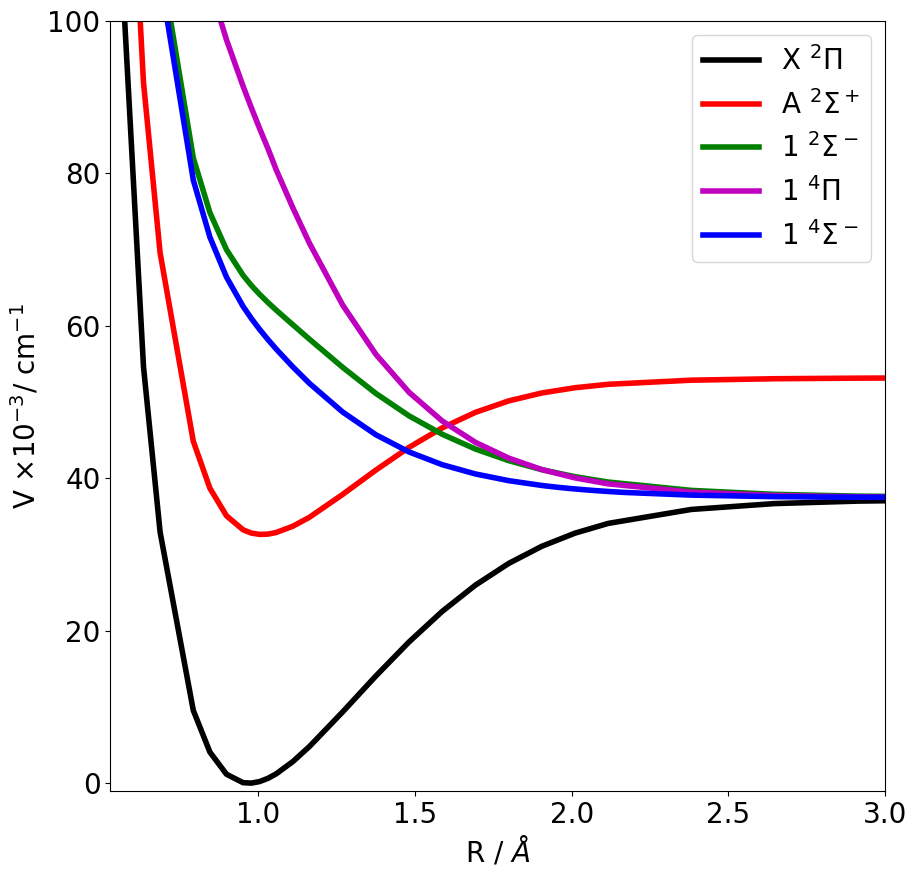
Figure 1: Ab initio potential energy curves for OH as computed in MolPro.

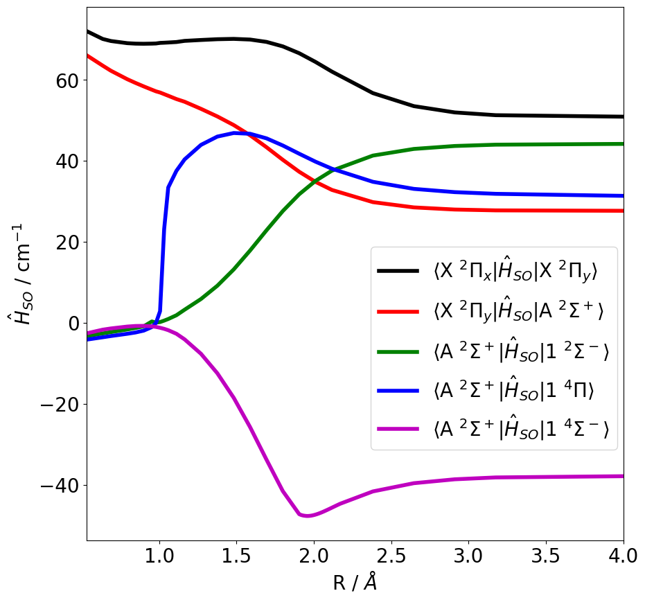
Figure 2: Diagonal and off-diagonal ab initio spin-orbit coupling curves of OH as computed in MolPro. The curves here also have an associated factor of $\pm i$.

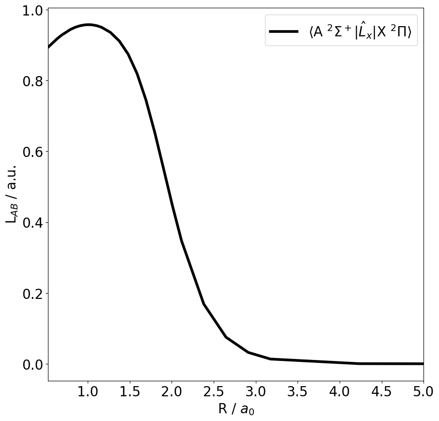
Figure 3: Ab initio L-uncoupling matrix elements for OH as computed in MolPro. In the cartesian coordinate system, there is a factor of $\pm i$.

III METHODS: Hydroxyl spectroscopic model

III.1 Global parameters

The curves produced above provide input to the nuclear motion code DuoDuo, an open-source Fortran 2009 program which provides variational solutions to the coupled rovibronic Schrödinger equations for a general open-shell diatomic molecule. Rovibronic energy levels and transitions are evaluated for the mutually perturbed X ${}^{2}\Pi$  and A ${}^{2}\Sigma^{+}$  states. However, the ab initio curves are insufficient for accurate reproduction and extrapolation of energy levels for this system despite the high level of ab initio  theory employed.

A number of global parameters need to be established before running a Duo calculation, they are as follows: The size of vibrational basis sets ($v_{\rm max}$) for each electronic state, the start ($r_{\rm min}$) and end ($r_{\rm c}$) of the calculation box, the number of grid points, and the maximum value for $J$. These considerations are made to ensure converged solutions for the energy levels. The start and end of the box was set to 0.53 Å and 8 Å respectively with a grid size of 801 points. The density of rovibronic states increases with energy. States near the top end of the available vibrational basis are unstable as they are asymmetrically perturbed by local rovibronic states due to lack of states at $v>v_{\rm max}$ which means that an insufficiently large $v_{\rm max}$ may lead to bound state solutions that may not be stable upon variation of the box size. $v_{\rm max}$ was selected for each electronic state iteratively. By extracting energy eigenvalues within the relevant fitting region for increasing $v_{\rm max}$, we can set $v_{\rm max}$ such that the energy levels are converged. This was found to occur when $v_{\rm max}^{X}\geq 110$ and $v_{\rm max}^{A}\geq 90$. The size of the vibrational basis sets were hence set to 110 and 90 for the X ${}^{2}\Pi$  and A ${}^{2}\Sigma^{+}$  states respectively. The maximum value for $J$, $J_{\textrm{max}}$, was set to 50.5.

III.2 Fitting

The PECs and coupling curves were refined by making constrained adjustments to parameters which describe them with respect to a set of observed data, which can be either empirical energy levels or transitions. These data are supplied by the recent MARVEL data set jt868. Energy level coverage of this dataset is summarized in table 2. Curve refinement is performed in Duo by least squares fitting to this data set.

Table 2: Coverage of MARVEL data set jt868 energy levels for the X ${}^{2}\Pi$  and A ${}^{2}\Sigma^{+}$  state of OH which have been used to refine ab initio PECs, SOCs and coupling constants for the production of a spectroscopic model.

v	$J_{\textrm{min}}$	$J_{\textrm{max}}$	Number of Levels
X ${}^{2}\Pi$
0	0.5	31.5	126
1	0.5	31.5	123
2	0.5	31.5	123
3	0.5	31.5	122
4	0.5	19.5	77
5	0.5	19.5	76
6	0.5	18.5	74
7	0.5	18.5	74
8	0.5	18.5	74
9	0.5	18.5	74
10	0.5	11.5	42
11	0.5	8.5	23
12	0.5	7.5	28
13	0.5	7.5	27
Total	0.5	31.5	1063
A ${}^{2}\Sigma^{+}$
0	0.5	31.5	64
1	0.5	28.5	58
2	0.5	19.5	40
3	0.5	26.5	54
4	0.5	19.5	40
5	0.5	7.5	15
6	0.5	8.5	17
7	0.5	7.5	16
8	0.5	9.5	19
9	0.5	8.5	17
Total	0.5	31.5	340
Grand Total			1403

Duo provides three types of fitting one can use; variation of parameters that describe a curve (sec. III.2.1), variation of parameters that describe a morphing function (morphing, see sec. III.2.2), and direct variation of individual grid points. In each case the optimization is based on a non-linear conjugate gradient method Duo with respect to an empirical data set.

III.2.1 Parameter variation fitting – pre-fitting

During parameter variation fitting, the curves must have some parametric form, and some initial set of parameters must be determined. For PECs, the form used in this study is the Extended Morse Oscillator (EMO)dPotFit; Duo, given by

$$V_{\rm EMO}(r)=T_{\rm e}+(A_{\rm e}-T_{\rm e})\left(1-e^{-\beta(r)(r-r_{\rm e})}\right)^{2}$$ (2)

where $T_{\textrm{e}}$ is the potential minimum, $D_{\rm e}=A_{\rm e}-T_{\rm e}$ is the dissociation energy relative to $T_{\textrm{e}}$ , $A_{\rm e}$ is the dissociation asymptote, $r_{\textrm{e}}$ is the equilibrium bond length, and $\beta(r)$ is a distance dependent exponent coefficient defined by the expansion term with coefficients $\beta_{i}$ with respect to the reduced coordinate $\xi_{p}$, first introduced by 84SuRaBo.method add are given by

$$\beta(r)=\sum^{N}_{i=0}\beta_{i}\xi_{p}(r)^{i};\quad N=\begin{cases}N_{R}&\textrm{for}~{}~{}r>r_{\rm e}\\ N_{L}&\textrm{for}~{}~{}r\leq r_{\rm e},\end{cases}$$ (3)

$$\xi_{p}(r)=\frac{r^{p}-r_{\rm e}^{p}}{r^{p}+r_{\rm e}^{p}};\quad p=\begin{cases}p_{R}&\textrm{for}~{}~{}r>r_{\rm e}\\ p_{L}&\textrm{for}~{}~{}r\leq r_{\rm e}.\end{cases}$$ (4)

This parametric form is flexible in that one can specify the behaviour around the equilibrium internuclear distance piece-wise using the parameters $N_{L}$, $N_{R}$, $p_{L}$, and $p_{R}$, where $N_{L}\leq N_{R}$. The value of $N_{R}$ hence defines the order of the expansion. This means one can establish a family of potential energy curves where the fundamental shape is determined by the set of parameters, $S$, where

$$S=\{p_{L},~{}p_{R},~{}N_{L},~{}N_{R}\};~{}~{}\{p_{L},~{}p_{R},~{}N_{L},~{}N_{R}\}\in\mathbb{Z},~{}N_{R}\geq N_{L}.$$ (5)

For a given $S$, one can then find $P$ which refines the shape to return appropriate energy levels, such that:

$$P=\{\beta_{i},~{}r_{\rm e},~{}T_{\rm e},~{}D_{\rm e}\};~{}~{}i\leq N_{R}.$$ (6)

When fitting a PEC in Duo, $S$ is fixed, and hence should be carefully chosen before optimizing $P$. Initial parameter selection has been performed by extending the method of 21MiTaTe.NaO. Given that the elements of $S$ are integers, one cannot use a standard optimization algorithm to optimize the values, and instead must solve the problem iteratively. The optimization of $S$ is therefore initiated by establishing the set,

$$\sigma_{S}= \{S_{0},...,S_{n}\}$$ (7)

$$\equiv \{\{p_{L_{0}},p_{R_{0}},N_{L_{0}},N_{R_{0}}\},...,\{p_{L_{n}},p_{R_{n}},N_{L_{n}},N_{R_{n}}\}\}$$ (8)

which contains $n$ elements of the set, $S$, as in Eq. (5) such that,

$$S_{i}\neq S_{j}~{}\forall~{}i,j;~{}~{}i\neq j.$$ (9)

This is the set of values of $p_{L}$, $p_{R}$, $N_{L}$, and $N_{R}$ over which we would like to test. The test consists of, for each $S_{i}$, finding the conjugate $P_{i}$ by least-squares fitting against the ab initio grid points in Python (code available on ExoMol GitHub). In each case we find the reduced $\chi^{2}$ test statistic, $\chi^{2}_{\nu}$ and search for the $S$, $P$ which return the lowest value. These parameters are then used as a starting point for fitting the PECs against experimental data in Duo. See table 3 for the $\sigma_{i}$ parameters for the X ${}^{2}\Pi$  and A ${}^{2}\Sigma^{+}$  states in this study.

Table 3: Parameters, $\sigma_{i}$ which best describe ab initio PECs of OH as calculated in sec II.1. Units in table footnote.

X ${}^{2}\Pi$		A ${}^{2}\Sigma^{+}$
$T_{\textrm{e}}$	0	$T_{\textrm{e}}$	32612.251248000
$r_{\textrm{e}}$	0.970655035	$r_{\textrm{e}}$	1.013454000
$A_{\textrm{e}}$	37269.126195730	$A_{\textrm{e}}$	53204.256220000
$p_{L}$	4	$p_{L}$	3
$p_{R}$	3	$p_{R}$	3
$N_{L}$	6	$N_{L}$	4
$N_{R}$	8	$N_{R}$	8
$\beta_{0}$	2.292052187	$\beta_{0}$	2.620396000
$\beta_{1}$	-0.019995181	$\beta_{1}$	0.169768000
$\beta_{2}$	0.198099686	$\beta_{2}$	0.465289000
$\beta_{3}$	0.231459916	$\beta_{3}$	0.552208000
$\beta_{4}$	-0.136025012	$\beta_{4}$	0.413921000
$\beta_{5}$	-0.639517770	$\beta_{5}$	-5.174652000
$\beta_{6}$	-0.277770706	$\beta_{6}$	9.999998000
$\beta_{7}$	6.274892232	$\beta_{7}$	3.333865000
$\beta_{8}$	-4.898195146	$\beta_{8}$	-9.999764000

Units:
$[T_{\rm e}]=\textrm{cm}^{-1}$
$[A_{\rm e}]=\textrm{cm}^{-1}$
$[r_{\rm e}]=$ Å
$[\beta_{i}]=$ Å${}^{-1}$

III.2.2 Morphing

As discussed above, morphing is another available technique for model refinement. In this case, one does not vary the curve in question directly, but instead varies a morphing function, $f_{\rm m}(r)$, which in turn, scales the ab initio curve, $f_{\rm ai}(r)$ 99MeHuxx.methods; 99SkPeBo.methods:

$$f_{\textrm{morphed}}(r)=f_{\rm ai}(r)f_{\rm m}(r).$$ (10)

As was done in 21MiTaTe.NaO, the Polynomial decay morphing function was used:

$$f_{\rm m}(r)=\sum^{N}_{k=0}{B_{k}z^{k}(1-\xi_{p})+\xi_{p}B_{\infty}},$$ (11)

where

$$z(r)=(r-r_{\rm ref})e^{-\beta(r-r_{\rm ref})^{2}-\gamma(r-r_{\rm ref})^{4}},$$

$\xi_{p}$ is as in Eq. (4), $B_{k}$ are variable expansion coefficients, $\beta$ and $\gamma$ are static coefficients typically set to $0.8$ and $0.02$ respectively, $B_{\infty}$ is typically set to unity to preserve the asymptotic behaviour of $f_{\rm ai}$, $N$ is the order of expansion, and $r_{\rm ref}$ is the expansion center. $r_{\rm ref}$ is set to the equilibrium bond length of the lower energy electronic state. When fitting Eq. 11, only the $B_{k}$ parameters are floated.

III.2.3 Constraining Curves

The asymptotic energy limit for all the curves in Fig. 1 was constrained by setting the value of $D_{\rm e}^{\rm X}$ to the experimental value of $D_{0}$ from 01Joens.OH with the added offset from the zero-point energy of the X ${}^{2}\Pi$ state, $E_{0}^{\rm X}$ calculated in Duo, hence

$$D_{\rm e}^{\rm X}=D_{0}+E_{0}^{\rm X}.$$ (12)

The remaining curves’ $D_{\rm e}$ where constrained with respect to $D_{\rm e}^{\rm X}$ such that their respective atomic limit spacings match that of NISTWebsite.

III.3 MARVEL Data Set and Quantum Number Conventions

jt868 collected 15938 rovibronic transitions from 45 sources and produced values for 1624 empirical rovibronic energy levels for the system of electronic states, X ${}^{2}\Pi$, A ${}^{2}\Sigma^{+}$, B ${}^{2}\Sigma^{+}$, C ${}^{2}\Sigma^{+}$. 12413 and 1403 of these transitions and empirical energy levels respectively concern the X ${}^{2}\Pi$ and A ${}^{2}\Sigma^{+}$  states. Table 2 presents the coverage of the MARVEL energy levels used in this study.

The complete set of quantum numbers used to characterise the MARVEL energy levels are the state label (X ${}^{2}\Pi$, A ${}^{2}\Sigma^{+}$, 1 ${}^{2}\Sigma^{-}$, …) total angular momentum, $J$, the vibrational quantum number, $v$, the rotationaless parity, $e/f$ and the projection of the total angular momentum on the molecular axis, $\Omega=\Sigma+\Lambda$, where, $\Sigma$ and $\Lambda$ are projections of the spin and orbital angular momenta on the molecular axis, respectively.

In line with the Hund’s case (a) conventions used in Duo, the following quantum numbers are used to characterize the rovibronic states, $|J,~{}v,~{}\tau,~{}\Sigma,~{}\Lambda,~{}\Omega,~{}State\rangle$ where $State$ is a counting number associated with the electronic states as ordered by potential minima, $T_{\rm e}$ and $\tau$ is the state parity $+/-$ (see jt632 for conversion between $e/f$ and $\tau$), which can be directly related to the MARVEL data set.

Instead of using the the Hund’s case (a) convention, many data sets on the rovibronic state of OH in the literature opt for the rotational quantum number $N$ and the fine structure components, $F_{1}$ and $F_{2}$ (Hund’s case (b)). In order to correlate these data with our MARVEL data set, their representations have been converted to the rigorous quantum labels $J$, $e/f$ using the following relations.
For the A ${}^{2}\Sigma^{+}$ state:

$$J=\begin{cases}N+\frac{1}{2}&\textrm{for}~{}~{}F_{1}\\ N-\frac{1}{2}&\textrm{for}~{}~{}F_{2}\end{cases}$$ (13)

$$e/f=\begin{cases}f&\textrm{for}~{}~{}F_{1}\\ e&\textrm{for}~{}~{}F_{2}\end{cases}$$ (14)

These relations arise, in particular, as the A ${}^{2}\Sigma^{+}$  state levels are generally presented using Hund’s case (b), hence the relation between $J$ and $N$, Eq. (13) and due to the common approximation,

$$E_{F_{1}}= BN(N+1)+\frac{1}{2}\gamma N$$ (15)

$$E_{F_{2}}= BN(N+1)-\frac{1}{2}\gamma(N+1).$$ (16)

Therefore, because $\gamma\ll B$, 16BrBeWe.OH where $B$ is the rotational constant and $\gamma$ is the spin-rotation constant,

$$E_{F_{1}}>E_{F_{2}}~{}~{}\forall~{}~{}N,J$$ (17)

and since the A ${}^{2}\Sigma^{+}$  state has only parity splitting as $\Lambda^{\textrm{A}}=0$, the $F_{1}$ and $F_{2}$ components correspond directly to $f$ and $e$ parities respectively (see 89Herzberg.adhoc_book).
For the X ${}^{2}\Pi$ state the relevant Hund’s case (a) approximation is:

$$E_{F_{1}}= B[(J+S)^{2}-\Lambda^{2}]-\frac{1}{2}(A-2B)$$ (18)

$$E_{F_{2}}= B[(J+S)^{2}-\Lambda^{2}]+\frac{1}{2}(A-2B)$$ (19)

Where $A$ is the diagonal spin-orbit coupling. This is applied for a given parity and correlates with the following relation 89Herzberg.adhoc_book:

$$E_{F_{1}}= E\left(\Omega=\frac{3}{2}\right)$$ (20)

$$E_{F_{2}}= E\left(\Omega=\frac{1}{2}\right)$$ (21)

The quantum number correlations for the quartet $1~{}(^{4}\Sigma^{-},^{4}\Pi)$ states have not been considered here as there are no experimental data which will require transformation.

IV Methods: Predissociation Lifetimes

OH predissociation lifetimes have long been the subject of theoretical and experimental studies, a summary of the available literature data has been provided in Table 4.

Table 4: Summary of predissociation lifetime data available from experimental and theoretical sources.

	Lifetime (ps)		$v$		$J$
Reference	Min	Max	Min	Max	Min	Max	Number of Lifetimes	Data Type
Experiment
05DePoDe 05DePoDe.OH	17	23	4	4	0.5	7.5	8	Predissociation Lifetimes
21SuZhZh 21SuZhZh.OH	14	130000	2	4	0.5	2.5	2	Predissociation Lifetimes
78BrErLy 78BrErLy.OH	33000	1110000	0	2	0.5	29.5	118	Total Lifetimes
91GrFa 91GrFa.OH	73	500	3	3	0.5	9.5	17	Predissociation Lifetimes
92HeCrJe 92HeCrJe.OH	62.89	312.50	3	3	0.5	13.5	27	Predissociation Rates
97SpMeMe 97SpMeMe.OH	29	167	3	3	4.5	14.5	20	Predissociation Rates
Theory
80SiBaLe 80SiBaLe.OH	2.95	428.16	3	9	Not $J$ Resolved		7	Predissociation Lifetimes
94KaSa 94KaSa.OH	3.32	6895.10	1	7	Not $J$ Resolved		7	Predissociation Lifetimes
99PaYa 99PaYa.OH	6000	9666000	0	4	0.5	30.5	107	Predissociation Lifetimes
Grand Total							313
This work	2.1	3600000	0	9	0.5	35.5	374	Predissociation Lifetimes

The data provided by 92HeCrJe.OH; 97SpMeMe.OH are given as predissociation rates and these have been inverted to return the required predissociation lifetimes. 78BrErLy.OH provides measurements of the total lifetime which is given by

$$\tau=\frac{\tau_{r}\tau_{p}}{\tau_{r}+\tau_{p}}$$ (22)

where $\tau_{r}$ and $\tau_{p}$ are the radiative and predissociative lifetimes respectively. As these values include also the radiative lifetime, we expect our calculations to be greater than these values. This is compounded by the fact that the predissociation in the region of $v\in[0,1,2]$ is less dominant than in $v\geq 3$.

A novel method for the calculation of predissociation lifetimes is applied in this section. The full details of the method will be available in Paper I, however, a brief summary of the method is given below.

IV.0.1 Energy resonances

An excited rovibronic state from A ${}^{2}\Sigma^{+}$  can predissociate via a spin-orbit interaction with a local repulsive state inducing the decay 21SuZhZh.OH; 87LeFr.OH; 95Le2.OH; 99PaYa.OH; 11LiZh.OH.

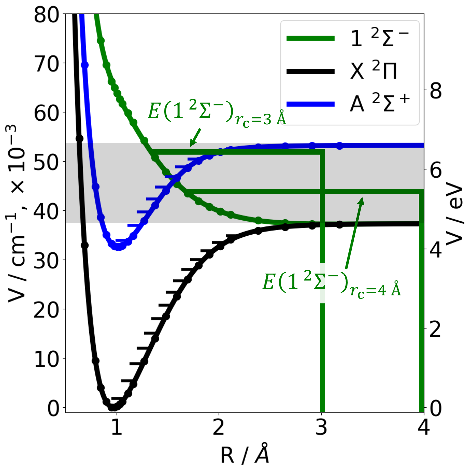
Figure 4: A toy model of OH consisting of the X ${}^{2}\Pi$, A ${}^{2}\Sigma^{+}$, and 1 ${}^{2}\Sigma^{-}$ electronic states. The two green levels, $E(1~{}^{2}\Sigma^{-})_{r_{\rm c}=3,4~{}\rm\mathring{A}}$ are continuum levels in the 1 ${}^{2}\Sigma^{-}$ electronic state with the same quantum numbers, however with different right-side box limits, $r_{\textrm{c}}$ . This highlights the box size dependence of repulsive state energy levels. The shaded region covers energy levels between $D_{\rm e}^{\rm X}$ and $D_{\rm e}^{\rm A}$.

In Fig. 4, the two green horizontal lines illustrate unbound state energy levels retrieved from Duo calculations with different right-side box limits, $r_{\textrm{c}}$ . Both sets of calculations are performed with the same left-side box limit $r_{\rm min}$. By construction the nuclear motion wavefunctions are only finite between $r_{\textrm{c}}$  and $r_{\rm min}$. The two green unbound state energy levels have the same quantum numbers $J,v,\tau,\Sigma,\Lambda,\Omega$, however, $E_{r_{\rm c}=3\rm\mathring{A}}$ returns a higher term value than $E_{r_{\rm c}=4\rm\mathring{A}}$. This is akin to the particle in a box, where increasing the size of the box compresses the distribution of energy levels closer to zero. Repeated calculations over varying $r_{\textrm{c}}$  in Duo for iso-numeric continuum energy levels exhibits a relationship where the term values decrease with $r_{\textrm{c}}$ , this is referred to as the energy profile of the continuum energy level.

The spin-orbit interaction between the 1 ${}^{2}\Sigma^{-}$and A ${}^{2}\Sigma^{+}$  states, $\langle^{2}\Sigma^{-}|\xi|^{2}\Sigma^{+}\rangle$, hence displaces the A ${}^{2}\Sigma^{+}$  state levels, which would otherwise be stable under variation of $r_{\textrm{c}}$ . This induced energy profile, allows us to study the predissociation characteristics of the quasi-bound A ${}^{2}\Sigma^{+}$  state levels.

The energy levels of interest for this study are found in the shaded region of Fig. 4. This covers 424 rovibronic energy levels in the A ${}^{2}\Sigma^{+}$  state.

The quantum number coverage for the relevant energy levels is presented in Table  5. Being above the first dissociation channel ($D_{\rm e}^{\rm X}$), each of these levels is quasi-bound and meta-stable with an associated characteristic lifetime, which we compute here. As discussed below, not all levels in the range had calculable predissociation lifetimes as per the method in Paper I, especially for levels with energy close to $D_{\rm e}^{\textrm{X}}$.

Table 5: Quantum number coverage for quasi-bound A ${}^{2}\Sigma^{+}$ state rovibronic levels.

v	$J_{\rm min}$	$J_{\rm max}$	Number of Levels	Number of Lifetimes
0	13.5	35.5	44	21
1	2.5	33.5	62	35
2	0.5	31.5	63	63
3	0.5	28.5	57	57
4	0.5	25.5	51	51
5	0.5	22.5	45	45
6	0.5	19.5	39	39
7	0.5	15.5	31	31
8	0.5	11.5	23	23
9	0.5	4.5	9	9
Total			424	374

Since repulsive electronic states have an infinitely dense set of continuum states, the position of the predissociating state, $|\textrm{A}^{2}\Sigma^{+},Q\rangle$, where $Q$ is the complete set of quantum numbers, $\{J,v,\tau\}$, has an uncertainty in the energy caused by the Pauli exclusion principle. This infinite set of states cannot be recovered using bound state methods for solving the Schrödinger equation for $r_{\rm c}\rightarrow\infty$, such as used by Duo, although more expensive scattering methods can be employed using Duo just for the inner regionjt755.

Here we approximate the continuum behaviour by discretizing the continuum jt840 and adapting the stabilization method 70HaYaHo.adhoc; 93MaRaTa.adhoc; 82BaSi.adhoc to characterize the quasi-bound states. In this method, infinite potential walls are assumed at the box limits $r_{\rm min}$ and $r_{\rm c}$, leading to bound-like rovibronic solutions even for continuum or quasi-bound states. By changing the position of the right-side wall $r_{\rm c}$, different continuum state term values can be generated and the uncertainty of the position of the quasi-bound states can be quantified as follows.

For a given box size defined by $r_{\rm c}-r_{\rm min}$ with a infinite potential wall, one can compute the term values $\tilde{E}_{|\textrm{A},Q\rangle}|_{r_{\rm c}}$ of the given set of quasi-bound, meta-stable states $\{$$|\textrm{A}^{2}\Sigma^{+},Q\rangle$$\}$. By varying $r_{\rm c}$, one can then establish a dependence of $E_{|\textrm{A},Q\rangle}$ on $r_{\rm c}$. In this study, $r_{\rm c}$ was varied between $r_{\rm c}=8$ and $8.999$ Å with the uniform spacing of 999 values ($\delta r_{\rm c}=0.001$ Å). This was done by repeating the Duo calculations while varying the right-side limit, $r_{\textrm{c}}$ (see Sec. III.1) and extracting the eigenenergies at each step. The number of the Duo sinc-DVR 92CoMixx.method grid points was increased as the box size was increased to maintain a uniform grid. Out of 999 runs, about 20 calculations failed, but these were simply ignored.

Figures 5 and 6 illustrate the box-size dependence for two A ${}^{2}\Sigma^{+}$  quasi-bound states of OH, $|\textrm{A}^{2}\Sigma^{+},J=0.5,v=4,e\rangle$ and $|\textrm{A}^{2}\Sigma^{+},J=0.5,v=2,e\rangle$ showing their ‘stabilisation’ character. The behavior is seen to be periodic with discontinuities at visually regular intervals and a central energy region in the middle. The typical resonance-like shapes are due to the interactions with continuum states. The discontinuities occur at the geometries where a crossing continuum energy level goes from pushing the quasi-bound level down to pushing it up and provide the energy level resonances from which we can calculate lifetimes. The line broadening parameter, $\Gamma$ and hence the lifetime of the state, $\tau\propto 1/\Gamma$, are associated with the widths of these resonances.

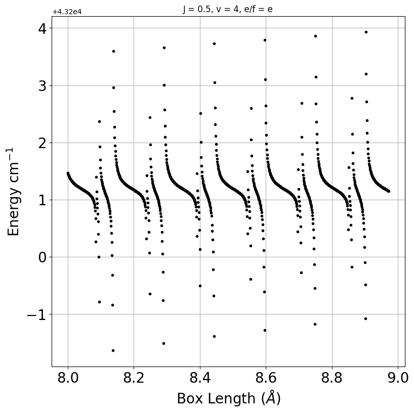
Figure 5: The term value of the $|\textrm{A}^{2}\Sigma^{+},J=0.5,v=4,e\rangle$ state as a function of the box length of the calculation in Duo, the variation of the energy is induced by crossings with energy levels in the repulsive states 1 ${}^{2}\Sigma^{-}$, 1 ${}^{4}\Sigma^{-}$, and 1 ${}^{4}\Pi$.

The interaction between A ${}^{2}\Sigma^{+}$ and the three continuum states 1 ${}^{2}\Sigma^{-}$, 1 ${}^{4}\Sigma^{-}$, 1 ${}^{4}\Pi$ are through the corresponding spin-orbit couplings from Fig. 2. There are several structures visible in Fig. 5, the asymptotes with the large wings and the asymptotes with the small wings. These substructures are caused by spin-orbit interactions with different electronic states, $1\,^{2}\Sigma^{-}$, $1\,^{4}\Sigma^{-}$, or $1\,^{4}\Pi$. The individual contributions can be resolved by performing calculations with only one of the three repulsive states and associated spin-orbit couplings present at a time, as illustrated in Fig. 6 for the $|\textrm{A}^{2}\Sigma^{+},J=0.5,v=2,e\rangle$ state (this state has been chosen for its simplicity). It shows that all three states contribute to the minor asymptotic wings but only the 1 ${}^{4}\Sigma^{-}$ state corresponds to the major wings. This makes the 1 ${}^{4}\Sigma^{-}$ state a bigger contributor to the predissociative decay for this particular state (due to a greater effect on the overall broadening), which is corroborated by the branching ratios reported by 11LiZh.OH who show that the 1 ${}^{4}\Sigma^{-}$ state is the primary branch.

For energy levels above $D_{\rm e}^{\rm X}$, X ${}^{2}\Pi$ state rovibronic levels become unbound and contribute to the perturbation of the A ${}^{2}\Sigma^{+}$ state level energies and hence provide an additional avenue for predissociation through the ground electronic state, see Fig. 7. The effect of predissociation through the X ${}^{2}\Pi$  state is small, and does not appear to have previously been reported. This effect cannot be isolated in our calculations, however, as removing the spin-orbit coupling between the X ${}^{2}\Pi$  and the A ${}^{2}\Sigma^{+}$  states shifts the energy levels too strongly (hundreds of cm${}^{-1}$) to be comparable.

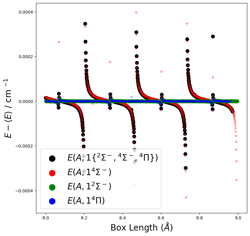
Figure 6: Term value of the $|\textrm{A}^{2}\Sigma^{+},J=0.5,v=2,e\rangle$ state as a function of the box length of the calculation in Duo. The different colors correspond to different spin-orbit contributions.

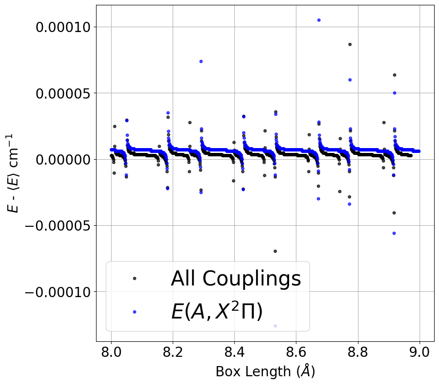
Figure 7: Term value of the $|\textrm{A}^{2}\Sigma^{+},J=13.5,v=1,f\rangle$ state as a function of the box length for a Duo calculation including the X ${}^{2}\Pi$ and A ${}^{2}\Sigma^{+}$  states only. The blue markers represent a shift in energy induced by the spin-orbit coupling between the X ${}^{2}\Pi$  and A ${}^{2}\Sigma^{+}$  states on the A ${}^{2}\Sigma^{+}$  state level.

IV.0.2 Statistical treatment

To calculate the predissociation lifetime from the above results, one calculates the integral normalised histogram of the energy data points centered around the mean $(E-\langle E\rangle)$, see Fig. 8 for an example. The binning of the histogram and the training of the Lorentzian parameters is non-trivial and is discussed in Paper I.

The probability function describing the system’s energy profile has the Lorentzian distribution 95Le1.OH:

$$L(\tilde{E};\tilde{E}_{0},\Gamma)=\frac{\frac{1}{\pi}(\frac{1}{2}\Gamma)}{(\tilde{E}-\tilde{E}_{0})^{2}+(\frac{1}{2}\Gamma)^{2}}$$ (23)

where $\tilde{E}_{0}$ is the peak position of the Lorentzian and $\Gamma$ is the full-width at half-maximum (line broadening parameter, in cm${}^{-1}$). The parameters $\{\tilde{E}_{0},\Gamma\}$ can be trained to best represent the histogram in Fig. 8, then the parameter $\Gamma$ is inverted via the relationship

$$\tau_{\rm p}=\frac{1}{2\pi c\Gamma}$$ (24)

where $c$ is the speed of light in $\textrm{cm s}^{-1}$.

There is an associated uncertainty to the fitting of the Lorentzian profile and this is discussed in Sec. IV.0.3. The Python package, binSLT was written to perform these calculations; it is available for download from https://github.com/exomol.

A visualisation of the Lorentzian-distributed energy histogram is shown in Fig. 8, where it is superimposed with the corresponding induced energy profile for the $|\textrm{A}^{2}\Sigma^{+},J=0.5,v=4,e\rangle$ state .

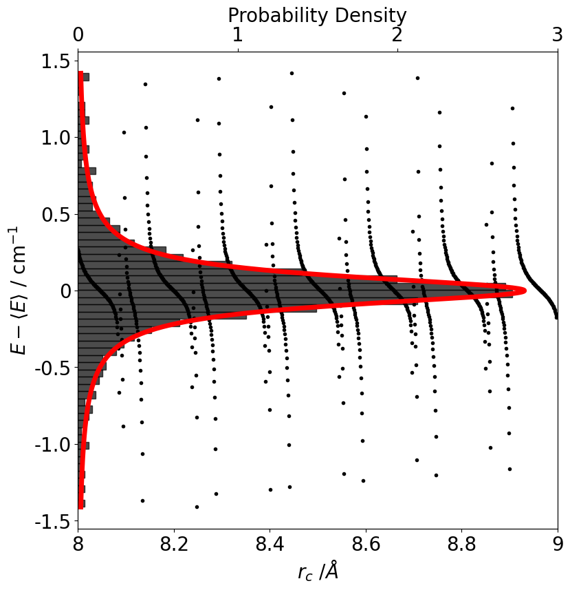
Figure 8: Plot of the energy against box length with the fitted histogram of energy points for the $|\textrm{A}^{2}\Sigma^{+},J=0.5,v=4,e\rangle$ state.

IV.0.3 Uncertainty Estimation

The largest uncertainties arise in states with long predissociation lifetimes. Here we will consider only the lifetimes which are shorter than the radiative lifetimes. As discussed in Paper I, the uncertainty is made up for four components, which are assumed independent and systematic and so are added to produce a final uncertainty $\Delta_{\tau}$

$$\Delta_{\tau}=\Delta_{M}+\Delta_{R}+\Delta_{B}+\Delta_{C},$$ (25)

where $\Delta_{M}$ is the uncertainty from convergence which is defined as $1-M$ where $M$ is the convergence level of the lifetime for a given state. This is typically the largest uncertainty and in cases of long lifetimes ($\tau_{p}>10^{5}$ ps) this can be as high as 20%. For lifetimes between $10^{4}$ and $10^{5}$ ps, $\Delta_{M}$ is evaluated at 10% and for lifetimes shorter than $10^{4}$ ps, this is found to be 5%.

$\Delta_{R}$ and $\Delta_{B}$ is the uncertainty from the positions of the repulsive and bound states’ energy levels. $\Delta_{B}$ is very difficult to measure directly, as it requires that the energy level positions of the bound states can be controlled with high precision in order to establish a relationship between the energy offset and the lifetime. This is, at the moment, infeasible. This has been estimated, however, by probing the effect the repulsive energy level positions have on the lifetimes. The asymptotic energy of the continuum states go to the O(${}^{3}$P) level, the same as the X ${}^{2}\Pi$ state. $D_{\rm e}(\textrm{X})$ has been experimentally measured to an uncertainty of 10 cm${}^{-1}$  by 01Joens.OH (see sec. III.2.3). Our continuum curves were shifted down by 20 cm${}^{-1}$  and the lifetimes for the predissociative states with $J\in[0.5,1.5]$ were re-computed and compared to the original model. This gives a conservative estimate on the uncertainty due to the position of the continuum curves, $\Delta_{R}$ of about 5%. The A ${}^{2}\Sigma^{+}$  state energy level position induced uncertainty, $\Delta_{B}$ is hence also estimated at 5%

$\Delta_{C}$ is the uncertainty of the numerical procedure excluding the problem of convergence. This is evaluated in situ for each state and has an average value over all states of approximately 2% in the case of OH. These uncertainties are distributed exponentially as is seen in Fig. 9.

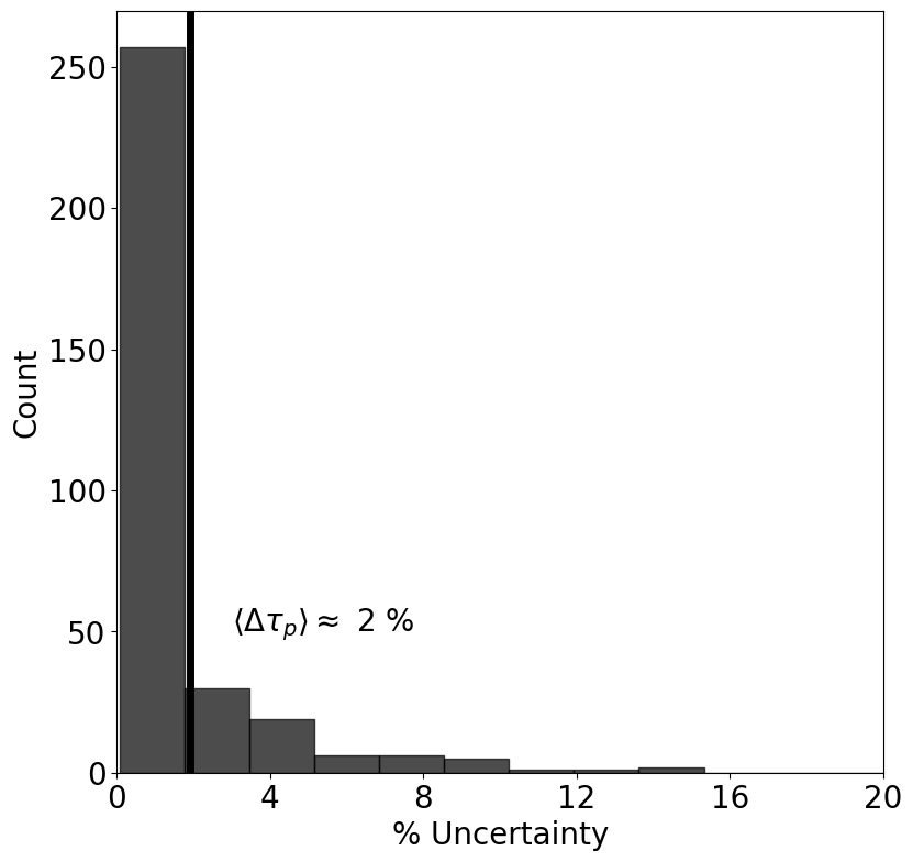
Figure 9: Distribution of percentage uncertainties in the lifetime induced by the computational procedure.

The lifetimes supplied in the supplementary material have been fully treated as in the methods described above and more completely, in Paper I. Tab. 6 gives a summary of the average uncertainties over different ranges of lifetimes in ps.

Table 6: Rules for attributing uncertainties for predissociation lifetimes calculated using the stabilization method for OH

Quantity	Value
Lifetime range / ps	$\left[0,10^{4}\right]$	$\left[10^{4},10^{5}\right]$	$\left[10^{5},10^{7}\right]$
Average Uncertainty / %	15+$\Delta_{C}$	20+$\Delta_{C}$	30+$\Delta_{C}$

V Results

V.1 Spectroscopic model parameters

Refinement of the curves representing the coupled model of the two states X ${}^{2}\Pi$  and A ${}^{2}\Sigma^{+}$  in Duo was performed by floating the parameters $r_{\rm e}({\rm X},{\rm A})$, $T_{\rm e}({\rm A})$, $\beta_{i}({\rm X,A})$ (PECs) and $B_{k}$ (spin-orbit and L-uncoupling curves)

Couplings to higher electronic states have not been considered for sake of simplicity in the model. Furthermore, couplings to repulsive electronic states for refinement of bound state energy levels have not been considered either. This has been done due to computational limitations as the box size of the calculation becomes an independent variable for the energy levels, see discussions above.

Along with the adjusted PECs and the morphed coupling curves, three more empirical, diagonal curves have been introduced to account for the aforementioned missing couplings jt632. These are the spin-rotation, $\gamma(X,A)$, the $\Lambda$-doubling $\alpha_{p2q}(X)$ and $q(X)$ 87BrChMe.adhoc, and the Born-Oppenheimer breakdown (BOB) radial property function 02LeHu.adhoc. The inclusion of such factors was necessary to refine the energy level reproduction without requiring the introduction of further electronic states or off-diagonal couplings. The Šurkus polynomial expansion function, $C(r)$ (see Eq. (26)), has been used as the parametric representation LEVEL,

$$C(r)=T_{\rm e}+(1-\xi_{p})\sum_{i\geq 0}B_{i}\xi_{p}^{i}+\xi_{p}B_{\infty}$$ (26)

where $\xi_{p}$ is the reduced coordinate in Eq. (4). The parameters $B_{i}$ and $B_{\infty}$ are floated.

The dissociation limits, $D_{\rm e}(\textrm{X,A})$ were fixed to the values $D_{\rm e}=D_{0}+\textrm{ZPE}$, where the zero point energy of the ground state was extracted from the Duo  calculation and found to be $\sim$ 1918 cm${}^{-1}$, $D_{0}(\textrm{X})$ was measured by 01Joens.OH to $\pm 10$ cm${}^{-1}$ $D_{\rm e}=D_{0}+\textrm{ZPE}$, while $D_{\rm e}(\textrm{A})$ was estimated by adding the difference in energy between the O(${}^{3}$P) and O(${}^{1}$D) atomic levels using values from the NIST Online Database NISTWebsite.

In Duo, one can fit spectroscopic model both against data sets of energy levels and of transitions in Duo. The process taken in this work was to fit it against the experimentally derived (MARVEL) energy levels by jt868.

A summary of fitted parameters is available in Tables 7, 8, 9 and a summary of uncertainties and RMS values is available in table 10. The Duo input file is given in the supplementary information.

Table 7: Summary of the PEC parameters obtained from least squares fitting the X ${}^{2}\Pi$  and A ${}^{2}\Sigma^{+}$  states of OH to MARVEL energy levels from jt868 in Duo Duo. All the figures are kept for the sake of preserving accuracy and reproducibility.

Parameter	X ${}^{2}\Pi$	A ${}^{2}\Sigma^{+}$
$T_{\textrm{e}}$	0	32663.976309068300
$r_{\textrm{e}}$	0.970020962666	1.005285998312
$A_{\textrm{e}}$	37501.792600000000	53369.654600000000
$p_{L}$	4	3
$p_{L}$	3	3
$N_{L}$	6	4
$N_{R}$	9	8
$\beta_{0}$	2.287411349533	2.625193503966
$\beta_{1}$	-0.008481205971	0.137874402944
$\beta_{2}$	0.138199166549	0.280685923916
$\beta_{3}$	-0.066491288959	0.687146152607
$\beta_{4}$	0.249817374269	1.374869049258
$\beta_{5}$	1.855331479551	-2.136036385410
$\beta_{6}$	2.083877071440	-14.858091727498
$\beta_{7}$	-21.177505781638	45.312091462135
$\beta_{8}$	34.392719961367	-32.477114187491
$\beta_{9}$	-16.859334102231

Table 8: Summary of the morphing parameters obtained from least squares fitting the X ${}^{2}\Pi$  and A ${}^{2}\Sigma^{+}$  states of OH to MARVEL energy levels and transitions from jt868 in Duo Duo.

Parameter	$\xi_{X}$	$\xi_{XA}$	$L_{XA}$
$r_{\textrm{e}}$	0.970655034638	0.970655034638	0.9704443874981
$\beta$	0.8	0.8	0.8
$\gamma$	0.02	0.02	0.02
$p$	6	6	2
$B_{0}$	1.008496273609	0.675170320954	0.772527250694
$B_{1}$	-0.504517931107	-0.799178556532	-0.649959182912
$B_{2}$	0.127429582028	-2.036097977961	-0.712564567820
$B_{\infty}$	1.000000000	1.000000000	1.000000000

Table 9: Summary of the empirical parameters obtained from least squares fitting the X ${}^{2}\Pi$  and A ${}^{2}\Sigma^{+}$  states of OH to MARVEL energy levels and transitions from jt868 in Duo Duo

	BOB(A ${}^{2}\Sigma^{+}$)	$\gamma_{X}$	$\gamma_{A}$	$\alpha_{p2q}$	$q$
$r_{\textrm{e}}$ (Å)	0.969785542585	0.969785542585	0.969785542585	0.969785542585	0.969785542585
$p$	2	2	2	2	2
$N$	3	3	3	3	3
$B_{0}$ (Å${}^{-1}$)	-0.013387427200	-0.082615835520	0.107579056717	0.081298271720	-0.015657399328
$B_{\infty}$ (Å${}^{-1}$)	-0.000897768443	0.029822159900	0.019259293154	-0.116865046681	0.016057094058

Table 10: Summary of the energy RMS values, in cm${}^{-1}$, obtained from least squares fitting the X ${}^{2}\Pi$  and A ${}^{2}\Sigma^{+}$  states of OH to MARVEL transitions from jt868 in Duo Duo

v	${\rm RMS}_{\rm X}$	${\rm RMS}_{\rm A}$
0	0.08	0.07
1	0.09	0.19
2	0.15	1.05
3	0.08	0.76
4	0.12	0.61
5	0.06	1.96
6	0.11	3.23
7	0.14	4.70
8	0.08	1.64
9	0.25	4.58
10	0.25
11	0.70
12	1.34
13	1.13
Whole State	0.33	1.79

V.2 Predissociation lifetimes

binSLT was used to compute the predissociation lifetimes of 374 quasi-bound A ${}^{2}\Sigma^{+}$ rovibronic states with follow up processing completed as further described in Paper I. 50 out of the allowed 424 states could not be processed as their energy profiles were too narrow and had insufficient resolution to compute $\Gamma_{\rm p}$.

A comparison with the lifetimes available in the literature (experiment and theory) and this work is illustrated in Fig. LABEL:fig:comparison, where the lifetime values are plotted as a function of $J$. The corresponding $J$-averaged percentage errors and their standard deviations are given in Table 11. A full tabulation of these data is available in the supplementary material for reference.

Table 11 shows that there is a satisfactory agreement between the lifetimes presented here and experiment; there is particularly good agreement for the cases where $v=3,4$, see Fig. LABEL:fig:comparison. In these cases, most results agreed within uncertainty (51/73 cases) and in regions where they did not agree, the mean percentage real difference in this region is $15\%$. The percentage real difference, ${}^{\rm R}\Delta_{\%}$ and percentage difference, $\Delta_{\%}$ here is defined as

$$D= \frac{|\Delta|-(\delta_{\rm calc}+\delta_{\rm lit})}{\tau_{\rm lit}}$$ (27)

$${}^{\rm R}\Delta_{\%}= \begin{cases}D&\textrm{for}~{}~{}D>0\\ 0&\textrm{otherwise}\end{cases}$$ (28)

$$\Delta_{\rm\%}= \frac{\tau_{\rm lit}-\tau_{\rm calc}}{\tau_{\rm lit}}\equiv\frac{\Delta}{\tau_{\rm lit}},$$ (29)

where $\tau_{\rm lit,calc}$ are the literature and calculated predissociation lifetimes respectively, $\Delta$ is the difference in those values, and $\delta_{\rm lit,calc}$ are the uncertainties quoted in the literature and calculated values respectively.

The noticeable exceptions to this are the lifetimes for $v\in[0,1,2]$ from 78BrErLy.OH. The experimental values in question here are total lifetimes rather than predissociation lifetimes. For $v<2$, radiative decay is the dominant source of broadening, hence the lifetimes of 78BrErLy.OH measurements should underestimate the predissociation lifetime. For $v=2$, predissociation is dominant, however radiative decay appears to be significant in the low $J$ region ($<6.5$).

One can consider the individual widths of the radiative and predissociative components, $\Gamma_{\rm r,p}$ and that the total width is $\Gamma=\Gamma_{\rm r}+\Gamma_{\rm p}$ and extract the dominance of the radiative decay, $R_{D}$ such that

$$R_{D}=\frac{\Gamma_{\rm r}}{\Gamma}$$ (30)

From our calculations, we compute $R_{D}$ and estimate the predissociation lifetime of 78BrErLy.OH through the relation

$$\tau_{\rm p}=\frac{\tau}{1-R_{D}}$$ (31)

and from this we are able to recover agreement within uncertainty with 78BrErLy.OH.

Table 11: Summary of comparison between predissociation lifetimes as calculated in this work and available literature values. Differences are averaged over $J$ for a given $v$. Only rotationally resolved literature lifetimes are compared here (see Table 4). Full comparison dataset provided in supplementary data.

Type	Ref	v	$\langle\Delta_{\%}\rangle$	Number	$C_{\rm A}$	$\langle^{\rm R}\Delta_{\%}\rangle$
Exp	05DePoDe05DePoDe.OH	4	-0.2	8	8	0.0
	21SuZhZh21SuZhZh.OH	2	-70.0	1	0	12.2
		4	-69.1	1	0	21.7
	78BrErLy78BrErLy.OH	0	-72.6	9	5	77.0
		1	-137.5	6	3	123.1
		2	-28.5	22	12	24.2
	91GrFa91GrFa.OH	3	-26.7	17	13	39.5
	92HeCrJe92HeCrJe.OH	3	-2.0	27	26	2.1
	97SpMeMe97SpMeMe.OH	3	-40.5	20	4	11.7
Theory	99PaYa99PaYa.OH	0	-76.7	11	4	34.9
		1	-77.1	9	3	27.0
		2	-87.2	23	0	33.0
		3	-48.0	35	1	25.6
		4	-15.3	21	12	6.1

The columns are as follows: Type = Experiment or Theory
Ref = Reference
$v$ = Vibrational quantum number
$\langle\Delta_{\%}\rangle$ = Average percentage difference
Number = number of $J$ resolved levels
$C_{A}$= Number of levels whose lifetimes agree within uncertainty
$\langle^{\rm R}\Delta_{\%}\rangle$: Average ${}^{\rm R}\Delta_{\%}$ for values which do not agree within uncertainty