Spinon Kondo lattice in quantum spin liquids

Abstract

Motivated by recent experimental observations of Kondo resonances in cobalt atoms on single layer 1T-TaSe₂, we theoretically investigate the effect of coupling a U(1) quantum spin liquid with a spinon Fermi surface to a lattice of Anderson impurities. Within the slave-rotor formalism, we find that above a critical coupling strength between the spin liquid and impurity lattice, the spinons hybridize to form heavy quasiparticles near the Fermi level, realizing a spinon Kondo lattice phase analogous to heavy fermion materials. Using the Bethe-Salpeter equation and accounting for emergent gauge fluctuations, we compute the spectral density and density of states, revealing the formation of spinon-chargon bound states in the spinon Kondo lattice phase. We characterize the thermodynamic and spectroscopic signatures of this phase, demonstrating specific heat and neutron scattering responses distinct from a pure quantum spin liquid. Our findings establish the spinon Kondo lattice as a framework to study the rich physics of spin liquids.

I Introduction

Quantum spin liquids (QSL) and resonating valence bond (RVB) states were initially introduced by Anderson as a physical mechanism to explain high $T_{c}$ superconductivity in cuprates [1, 2]. QSL is a quantum paramagnetic Mott insulator phase which evades a long-range magnetic order even at zero temperature. Instead, the QSL is an exotic quantum phase of quantum matter described by topological order [3, 4] and many-body long-range entanglement [5]. The emergent gauge fields and symmetry classification by projective symmetry group are used to reveal the existence of a variety of quantum phases with the same symmetry yet with distinct properties. Among all, the U(1) quantum spin liquid with spinon Fermi surface is a spin liquid where spinons are gapless forming a Fermi surface and are coupled with emergent U(1) gauge fields [6, 7]. Due to the presence of spin-charge separation in Mott insulators, the elementary dynamical units are fractionalized to spinons and chargons [8, 9, 10, 6]. The spinons are charge neutral spin-1/2 fermion and chargons are spinless boson with electron change $-e$. Therefore, this U(1) quantum spin liquid and some of their physical characteristics resemble those of Fermi liquids. For example, the entanglement entropy in real space follows a logarithmic area law $S_{E}\sim L\log(L)$, where $L$ represents the boundary length, for both the U(1) quantum spin liquid and Fermi liquid [11, 12]. On the other hand, the coupling of conventional metals to localized magnetic moments gives rise to the Kondo bound state and the Kondo effect [13, 14, 15], characterized by a prominent Kondo resonance peak in the electronic spectrum.

The recent experimental observation of resonant states in cobalt atoms on single-layer 1T-TaSe₂ provided evidence of the spinon Kondo effect in a spin liquid [16]. It has been found that the coupling of the U(1) quantum spin liquid with impurities leads to the emergence of the spinon Kondo effect [17]. Although the spin liquid is an insulator, it exhibits properties similar to the electronic Kondo effect, with the spinon spectrum resembling the electron spectrum in the Kondo effect. Resonance peaks appear at the inner edges of the upper and lower Hubbard bands in the spin liquid, which are attributed to the formation of spinon-chargon bound states induced by the emergent gauge fields near the impurity. Therefore, despite the complexity of the U(1) quantum spin liquid compared to the Fermi liquid, it often exhibits similarities due to the presence of a Fermi surface in its internal dynamical units.

The Kondo lattice model is formed by coupling a Fermi liquid to a lattice of magnetic ions. The hybridization between the latter and the host electrons dissolves the impurity spins into the Fermi liquid, endowing them with electric charge [18]. This process gives rise to the formation of heavy fermion quasiparticles [19, 15, 20], known as heavy Fermion materials, characterized by a significant increase in the effective mass of the quasiparticles. Furthermore, if the magnetic interaction between ions is taken into account and assuming they form a spin liquid, a phase transition from a heavy fermion phase with a large Fermi surface to a fractionalized Fermi liquid (FL^∗) phase occurs as the Kondo interaction strength decreases [21, 22, 23].

Motivated by recent scanning tunneling spectroscopy measurements on single-layer 1T-TaSe₂ and the observation of Kondo resonances [16], we speculate that similar phenomena to the Kondo lattice may arise when a quantum spin liquid is coupled with a lattice of magnetic ions. The main message of our work is to introduce and convey the concept of the spinon Kondo lattice phase. We introduce a model consisting of a quantum spin liquid coupled to a lattice of Anderson impurities (AL) and explore its connection to heavy fermion effects. In particular, we aim to answer the following questions: i) how does the Anderson impurity lattice affect the spinon Fermi surface and the single-particle spectra of spinons and chargons? ii) does the coupling between the impurity lattice and the U(1) quantum spin liquids give rise to new quantum phases? iii) what is the influence of emergent gauge fields in the U(1) quantum spin liquids on the system? iv) what are the possible experimental signatures of phases? To address these questions, we organize the paper as follows. Sec. II begins with the Hubbard model coupled with Anderson impurity lattice and analyzes the phases using the slave rotor method and mean-field approximation, elucidating the quantum phase transitions and parton single-particle spectra. In Sec. III, we investigate the physical electron excitations through parton Green’s functions and the Bethe-Salpeter equation, taking into account the effects of emergent gauge fields on the Green’s functions and single-electron spectrum. In Sec. IV, we explore the thermodynamic properties and relevant observables of our model. The Sec. V summarizes the main findings. The details of derivations of some expressions are relegated to Appendices.

II Slave rotor approach to Anderson impurity lattice

The Hamiltonian of the Hubbard model, coupled to an impurity lattice [15], in the spin liquid phase can be expressed as follows:

$$H= \sum_{i,j,\sigma}t_{ij}c_{i,\sigma}^{\dagger}c_{j,\sigma}+\sum_{i\sigma}\epsilon_{d}d_{i,\sigma}^{\dagger}d_{i,\sigma}+V\sum_{i\sigma}c_{i,\sigma}^{\dagger}d_{i,\sigma}+\mathrm{h.c.}$$

$$+\frac{U_{\mathrm{QSL}}}{2}\sum_{i}(n_{ic}-1)^{2}+\frac{U}{2}\sum_{i}(n_{id}-1)^{2},$$ (1)

where $c(d)$ are fermionic annihilation operators of electrons residing on sites of the lattice of itinerant electrons (Anderson impurities), and the corresponding number operators are $n_{ic}=\sum_{\sigma}c_{i,\sigma}^{\dagger}c_{i,\sigma}$ and $n_{id}=\sum_{\sigma}d_{i,\sigma}^{\dagger}d_{i,\sigma}$. In this expression, $t_{ij}$ is the hopping integral, $\epsilon_{d}$ is the energy of the impurity electron, $\sigma=\{\uparrow,\downarrow\}$ is the spin index, $V$ is the strength of the coupling between the itinerant and impurity electrons. $U_{\mathrm{QSL}}$ is the Hubbard interaction between host itinerant electrons, and we assume that it is strong enough to drive the host system into a spin liquid phase. $U$ is the Coulomb repulsion between electrons on a single Anderson impurity.

We utilize the slave rotor construction [9, 10] to express the electron operators as composites of spinon and chargon operators: $c_{i,\sigma}=f_{i,\sigma}X_{i}^{\dagger}$ and $d_{i,\sigma}=a_{i,\sigma}Y_{i}^{\dagger}$, where $X_{i}=e^{-i\theta_{i}}$ and $Y_{i}=e^{-i\phi_{i}}$ represent the field operators of spinons and chargons, respectively. Substituting these relations into Eq. (1), we obtain:

$$H= \sum_{i,j,\sigma}t_{ij}f_{i,\sigma}^{\dagger}f_{j,\sigma}X_{j}^{\dagger}X_{i}+\mathrm{h.c.}-\sum_{i\sigma}\left(\mu+h_{1,i}\right)f_{i,\sigma}^{\dagger}f_{i,\sigma}$$

$$+\sum_{i\sigma}\left(\epsilon_{d}-h_{2,i}\right)a_{i,\sigma}^{\dagger}a_{i,\sigma}+V\sum_{i\sigma}f_{i,\sigma}^{\dagger}a_{i,\sigma}Y_{i}^{\dagger}X_{i}+h.c.$$

$$+U_{\mathrm{QSL}}\sum_{i}P_{i}^{\dagger}P_{i}+i\sum_{i}h_{1,i}P_{i}X_{i}-i\sum_{i}h_{1,i}X_{i}^{\dagger}P_{i}^{\dagger}$$

$$+U\sum_{i}Q_{i}^{\dagger}Q_{i}+i\sum_{i}h_{2,i}Q_{i}Y_{i}-i\sum_{i}h_{2,i}Y_{i}^{\dagger}Q_{i}^{\dagger}$$

$$+\sum_{i}\lambda_{1,i}\left(X_{i}^{\dagger}X_{i}-1\right)+\sum_{i}\lambda_{2,i}\left(Y_{i}^{\dagger}Y_{i}-1\right)$$

$$+\sum_{i}h_{1,i}+\sum_{i}h_{2,i}.$$ (2)

Here, $P_{i}$ and $Q_{i}$ are the momenta conjugated to the coordinates $X_{i}$ and $Y_{i}$, respectively. $\mu$ is the chemical potential of itinerant electrons. $\lambda_{1,i}$ and $h_{1,i}$ are the Lagrange multipliers that ensure the constraints $X_{i}^{\dagger}X_{i}=1$ and $L_{X,i}=i(X_{i}P_{i}-X_{i}^{\dagger}P_{i}^{\dagger})=\sum_{\sigma}f_{i,\sigma}^{\dagger}f_{i,\sigma}-1$ hold. Similarly, $\lambda_{1,i}$ and $h_{1,i}$ regarding $Y_{i}$ fields are defined. We use the Hubbard-Stratonovich transformation to decompose the four-field terms with auxiliary fields. The Eq. (2) then becomes $H=H_{\mathrm{QSL}}+H_{\mathrm{AL}}+H_{\mathrm{c}}$, where $H_{\mathrm{QSL}}$ describes the host electron layer with

$$H_{\mathrm{QSL}} =\sum_{i,j,\sigma}t_{ij}\chi_{ji}^{X}f_{i,\sigma}^{\dagger}f_{j,\sigma}+\mathrm{h.c.}-\sum_{i,\sigma}\left(\mu+h_{1,i}\right)f_{i,\sigma}^{\dagger}f_{i,\sigma}$$

$$+\sum_{i,j}\chi_{ij}^{f}X_{j}^{\dagger}X_{i}+U_{\mathrm{QSL}}\sum_{i}P_{i}^{\dagger}P_{i}$$

$$+\sum_{i}\lambda_{1,i}(X_{i}^{\dagger}X_{i}-1)-\sum_{i,j}\chi_{ji}^{X}\chi_{ij}^{f},$$ (3)

$H_{\mathrm{AL}}$ describes the second layer consisting of Anderson impurities with

$$H_{\mathrm{AL}}= \sum_{i,\sigma}\left(\epsilon_{d}-h_{2}\right)a_{i,\sigma}^{\dagger}a_{i,\sigma}+\sum_{i}\lambda_{2,i}\left(Y_{i}^{\dagger}Y_{i}-1\right)+\sum_{i}h_{2,i}$$

$$+U\sum_{i}Q_{i}^{\dagger}Q_{i}+i\sum_{i}h_{2,i}Q_{i}Y_{i}-i\sum_{i}h_{2,i}Y_{i}^{\dagger}Q_{i}^{\dagger},$$ (4)

and $H_{\mathrm{c}}$ describes the coupling between the two layers

$$H_{\mathrm{c}}=-\sum_{i}u_{i}Y_{i}^{\dagger}X_{i}+\sum_{i,\sigma}w_{i}f_{i,\sigma}^{\dagger}a_{i,\sigma}+\sum_{i}\frac{2u_{i}w_{i}}{V}.$$ (5)

In the mean-field approximation, the coupled fields and Lagrange multipliers satisfy the following self-consistent equations at the saddle point:

$$u= -\frac{2V}{\beta N}\sum_{\bm{k},n}G(a,f^{\dagger},i\omega_{n},\bm{k},\sigma),$$ (6)

$$w= -\frac{V}{\beta N}\sum_{\bm{k},n}G(X,Y^{\dagger},i\nu_{n},\bm{k}),$$ (7)

$$1= -\frac{1}{\beta N}\sum_{\bm{k},n}G(Y,Y^{\dagger},i\nu_{n},\bm{k})e^{i\nu_{n}0^{+}},$$ (8)

$$0= -\frac{1}{2U\beta N}\sum_{\bm{k},n}i\nu_{n}G\left(Y,Y^{\dagger},i\nu_{n},\bm{k}\right)\left[e^{i\nu_{n}0^{+}}+e^{-i\nu_{n}0^{+}}\right]$$

$$+\frac{h_{2}}{U}+\frac{1}{\beta N}\sum_{\bm{k},n}G\left(a,a^{\dagger},i\omega_{n},\bm{k},\sigma\right)-\frac{1}{2}.$$ (9)

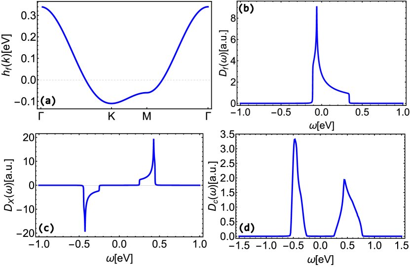
Figure 1: (a) Spinon dispersion relation of isolated U(1) spin liquid, along path through symmetry points $\Gamma,\mathrm{K},\mathrm{M},\Gamma$ in triangular lattice Brillouin Zone. (b), (c) The spectral functions of spinons and chargons of U(1) spin liquid respectively. The spectral functions is obtained from $D(\omega)=-\frac{1}{\pi N}\sum_{\bm{k}}\mathrm{Im}G(\omega+i0^{+},\bm{k})$. (d) Electron spectral function, which is obtained by convolution of spinons and chargons’ Green’s functions.

In these equations, we set $h_{2,i}=0$, since $L_{Y,i}=\sum_{\sigma}a_{i,\sigma}^{\dagger}a_{i,\sigma}-1=0$ is always a solution of Eq. (9), which means that the impurity lattice still maintains the single-occupation state of the electrons. The constant $N$ is the number of unit cells and $\beta=1/k_{B}T$ is the inverse temperature. $\omega_{n}=(2n+1)\pi/\beta$ and $\nu_{n}=2n\pi/\beta$ are the fermionic and bosonic Matsubara frequencies, respectively. Additionally, we have used the spin liquid mean-field Hamiltonian that matches the recent experiment on single-layer 1T-TaSe₂ [16]:

$$H_{\mathrm{QSL}}=\sum_{\bm{k},\sigma}h_{f}(\bm{k})f_{\bm{k},\sigma}^{\dagger}f_{\bm{k},\sigma}+\sum_{k}\omega_{X}^{2}(\bm{k})X_{\bm{k}}^{\dagger}X_{\bm{k}}+U_{\mathrm{QSL}}\sum_{\bm{k}}P_{\bm{k}}^{\dagger}P_{\bm{k}},$$ (10)

where spinon energy $h_{f}(\bm{k})=t_{F}\gamma(\bm{k})-\mu$, $\omega_{X}(\bm{k})=\sqrt{-t_{X}\gamma(\bm{k})+\lambda_{1}}$ is chargon frequency, and nearest neighbor form factor $\gamma(\bm{k})=2(2\cos\frac{1}{2}k_{x}a\cos\frac{\sqrt{3}}{2}k_{y}a+\cos k_{x}a)$ and $a$ is lattice constant. Here, $t_{F}=0.05~{}\mathrm{eV}$, $t_{X}=0.019~{}\mathrm{eV}$ are spinon and chargon hopping, $\mu=-0.04~{}\mathrm{eV}$ is the spinon chemical potential, and local interaction $U_{\mathrm{QSL}}=0.775~{}\mathrm{eV}$, $\lambda_{1}=0.157~{}\mathrm{eV}$ is Lagrange multiplier. The relation between Mott gap and parameter $\lambda_{1}$ are $\Delta_{g}=\sqrt{U_{\mathrm{QSL}}(\lambda_{1}-6t_{F})}=0.25~{}\mathrm{eV}$. The Green’s functions in equations above are (see Appendix B for details):

$$G^{0}(f,f^{\dagger},i\omega_{n},\bm{k},\sigma)=\frac{1}{i\omega_{n}-h_{f}(\bm{k})},$$ (11)

$$G^{0}(a,a^{\dagger},i\omega_{n},\sigma)=\frac{1}{i\omega_{n}-\epsilon_{d}},$$ (12)

$$G(f,a^{\dagger},i\omega_{n},\bm{k},\sigma)=\frac{wVG^{0}(f,f^{\dagger},i\omega_{n},\bm{k},\sigma)}{i\omega_{n}-\epsilon_{0}-w^{2}G^{0}(f,f^{\dagger},i\omega_{n},\bm{k},\sigma)},$$ (13)

$$G^{0}(X,X^{\dagger},i\nu_{n},\bm{k})=\frac{-1}{\frac{\nu_{n}^{2}}{U_{QSL}}+\omega_{X}^{2}(\bm{k})},$$ (14)

$$G(X,Y^{\dagger},i\nu_{n},\bm{k})=\frac{uG^{0}(X,X^{\dagger},i\omega_{n},\bm{k})}{\frac{\nu_{n}^{2}}{U}+\lambda_{2}+u^{2}G^{0}(X,X^{\dagger},i\nu_{n},\bm{k})},$$ (15)

$$G(Y,Y^{\dagger},i\nu_{n},\bm{k})=\frac{-1}{\frac{\nu_{n}^{2}}{U}+\lambda_{2}+u^{2}G^{0}(X,X^{\dagger},i\nu_{n},\bm{k})}.$$ (16)

II.1 Uncoupled model: the spin liquid phase

First, let us set $V=0$, the uncoupled layers. As pointed out earlier, we consider the limit of a large $U_{\mathrm{QSL}}/t$ ensuring that the system is deep within the Mott insulator phase with a spin liquid ground state. Within the slave-rotor framework, the insulating Mott phase is characterized by the vanishing quasiparticle weight given by the expectation value of the rotor field $Z=\langle X\rangle$ [9, 10, 24, 25], implying that the charge is stripped off electrons. In Fig. 1, we show the electronic structure of the Mott phase. Fig. 1(a) depicts the energy band dispersion of the spinons $h_{f}(\bm{k})$ on the triangular lattice. The Fermi level corresponding to half-filling is shown by a dashed line, and it is seen that the spinons form a Fermi surface. Fig. 1(b) shows the corresponding density of states of spinons $D_{f}(\omega)=(1/N)\sum_{\bm{k}}A_{f}(\omega,\bm{k})$ where $A_{f}(\omega,\bm{k})=-(1/\pi)\mathrm{Im}G^{0}(f,f^{\dagger},\omega+i0^{+},\bm{k},\sigma)$ is the spinon spectral density. The density of states of chargons $D_{X}(\omega)=(1/N)\sum_{\bm{k}}A_{X}(\omega,\bm{k})$ with $A_{X}(\omega,\bm{k})=-(1/\pi)\mathrm{Im}G^{0}(X,X^{\dagger},\omega+i0^{+},\bm{k})$ is shown in Fig. 1(c). The Mottness of the original electrons is, however, given by the spectral density of the convoluted spinon and chargon Green’s functions, $D_{c}(\omega)=(1/N)\sum_{\bm{k}}A_{c}(\omega,\bm{k})$ with $A_{c}(\omega,\bm{k})=-(1/\pi)\mathrm{Im}G^{0}(c,c^{\dagger},\omega+i0^{+},\bm{k},\sigma)$, where $G^{0}(c,c^{\dagger},i\omega_{n},\bm{k},\sigma)=\beta^{-1}\sum_{\nu_{m}}G^{0}(f,f^{\dagger},i\omega_{n}+i\nu_{m},\bm{k},\sigma)G^{0}(X,X^{\dagger},i\nu_{m},\bm{k})$. The density of states $D(\omega)$ is shown in Fig. 1(d), where the formation of upper and lower Hubbard bands is clearly seen.

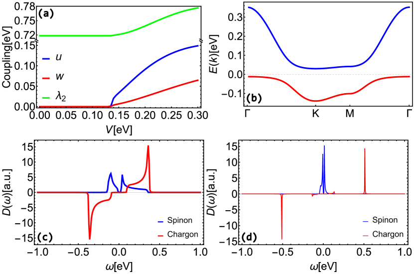
Figure 2: (a) The mean field parameters $u$ and $w$ as a function of the coupling $V$. (b) The spinon dispersion relation in spinon Kondo lattice phase. (c) Spinon and chargon spectral functions of spin liquid part in spinon Kondo lattice phase. (d) Spinon and chargon spectral functions of Anderson lattice part in spinon Kondo lattice phase.

II.2 Spinon Kondo lattice phase

Having established the spin liquid phase on the triangular lattice as described in the preceding subsection, we now consider the hybridization of the spin liquid phase with a lattice of Anderson impurities. The coupling strength is given by $V\neq 0$ (see Eq. (1)), whose effects are encapsulated in the fields $u_{i}$ and $w_{i}$ in Eq. (5), which determine the hybridization between the spinons (chargons) of the spin liquid phase and the spinons (chargons) on the Anderson impurity, respectively. To examine the effects of $V\neq 0$, we solved the self-consistent equations in Eqs. (6)-(7) along with the constraints in (8) and (9) numerically.

The variation of the hybridization fields $u$ and $w$ as a function of the coupling strength is shown in Fig. 2(a). There is a critical coupling strength $V_{c}$ beyond which the hybridization fields $u$ and $w$ acquire nonzero values. When $V<V_{c}$, $u$ and $w$ are equal to zero, indicating that the system consists of two separate layers; the spin liquid phase and the Anderson impurity lattice are uncoupled. For $V>V_{c}$, $u$ and $w$ are greater than zero, placing the system in the hybridized phase characterized by heavy spinons near the Fermi level, where the dispersion becomes nearly flat, as seen in Fig. 2(b). This phase is termed a spinon Kondo lattice phase. It is important to note the distinct difference between the spinon Kondo lattice phase and the normal heavy fermions in the Kondo lattice model. In the latter, a normal metal is antiferromagnetically coupled to a lattice of magnetic impurities as $J\sum_{i}c_{i}^{\dagger}\bm{\sigma}c_{i}\cdot\bm{S}_{i}$. Here, the coupling strength $J$ is relevant, and the model transitions to a heavy fermion model as soon as $J\neq 0$. However, in our model, there is a critical value of coupling strength, $V_{c}$, where the phase transition occurs.

Furthermore, the spinon Kondo lattice phase is characterized by two spinon bands separated by a small gap, as shown in Fig. 2(b), analogous to the Kondo insulator phase. Indeed, the hybridized bands open a gap between them. Since the spin liquid phase and the impurity lattice are both singly occupied, the spinon occupation number (1+1) mod 2 is equal to zero, leading the system to form a spinon Kondo insulator.

III Spinon-chargon bound states

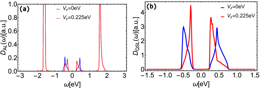
Figure 3: (a) Spectral function of electron for Anderson lattice part in spinon Kondo lattice phase, where blue and red line refer the interaction strength $V_{\bm{r}}=0\ \mathrm{eV}$ and $V_{\bm{r}}=0.225\ \mathrm{eV}$ respectively. (b) Spectral function of electron for QSL part in spinon Kondo lattice phase, where blue and red line refer the same meaning as (a).

In a U(1) quantum spin liquid, there exists an emergent U(1) gauge symmetry between the spinons and chargons. At low energies, the corresponding U(1) gauge field is noncompact and mediates a Coulomb potential [26, 27] with the assumption of deconfined quantum spin liquid, which tends to bind the spinons and chargons together into electrons [8, 7, 27, 17].To analyze bound states, we employ the Bethe-Salpeter equation to calculate the electron Green’s functions. We define new field operators $\psi_{s}(i\omega_{n},\bm{k},\sigma)=(a(i\omega_{n},\sigma),f(i\omega_{n},\bm{k},\sigma))^{T}$, $Z_{c}(i\nu_{n},\bm{k})=(Y(i\nu_{n}),X(i\nu_{n},\bm{k}))^{T}$ for spinons and chargons, respectively.

In the ladder approximation, the Bethe-Salpeter equation is given by [28, 29, 30]:

$$G_{\psi_{e}}(k_{1})= -(\beta N)^{-1}\sum_{q}G_{\psi_{s}}(k+q)\otimes G_{Z_{c}}(q)$$

$$\times\left(\mathbf{1}_{2}-(\beta N)^{-1}\sum_{q}K_{p}^{*}\left(i\nu_{n}\right)G_{\psi_{s}}(k+q)\otimes G_{Z_{c}}(q)\right)^{-1},$$ (17)

where $k=(i\omega_{n},\bm{k})$, $q=(i\nu_{n},\bm{q})$, the Green’s functions $G_{\psi_{e/s}}(k)$ and $G_{Z_{c}}(q)$ are defined as $G_{\psi_{e/s}}(k)=G(\psi_{e/s},\psi_{e/s}^{\dagger},i\omega_{n},\bm{k},\sigma)$, and ( $G_{Z_{c}}(q)=G(Z_{c},Z_{c}^{\dagger},i\nu_{n},\bm{q})$, respectively. In this context, $\otimes$ denotes the Kronecker product, resulting in a $4\times 4$ matrix, and we consider only the $i,j\in\{1,4\}$ block. $\mathbf{1}_{2}$ represents the two-dimensional identity matrix. The $2\times 2$ matrix $K^{*}(i\nu_{n})$ is the approximate two-body interaction kernel with zero entries except for $[K^{*}(i\nu_{n})]_{22}=-\frac{i\nu_{n}}{U_{QSL}}V_{\bm{r}}$. We focus on the screened Coulomb potential at the same lattice site, where $V_{\bm{r}}=\varLambda_{f}$ , as detailed in Appendix E. Here, $\varLambda_{f}$ is defined as the spinon half bandwidth, $\varLambda_{f}=(\max[h_{f}(\bm{k})]-\min[h_{f}(\bm{k})])/2$.

The electron Green’s functions for the Anderson lattice and the spin liquid part are denoted as $G_{\mathrm{AL}}$ and $G_{\mathrm{QSL}}$, respectively, and are given by $G_{\mathrm{AL/QSL}}=\left[G(\psi_{e},\psi_{e}^{\dagger},\omega+i0^{+},\bm{k}_{1},\sigma)\right]_{11/22}$. Subsequently, we derive their spectral densities $A_{\mathrm{AL/QSL}}(\omega,\bm{k}_{1})=-\frac{1}{\pi}\mathrm{Im}\left[G(\psi_{e},\psi_{e}^{\dagger},\omega+i0^{+},\bm{k}_{1},\sigma)\right]_{11/22}$ and the density of states for each lattice as $D_{\mathrm{AL/QSL}}(\omega)=-\frac{1}{\pi N}\sum_{\bm{q},\sigma}A_{\mathrm{AL/QSL}}(\omega,\bm{k}_{1})$. The results are illustrated in Fig. 3. Notably, the very sharp peaks near $\omega\simeq 1.8\ \mathrm{eV}$ correspond to the lower and upper Hubbard excitations on the Anderson impurity, which remain unaffected by the Coulomb potential. However, the middle bands, which arise from hybridization with the spin liquid, are influenced by the formation of the bound state. The impact of the Coulomb potential and the spinon-chargon bound states is more pronounced in the density of states of the parent quantum spin liquid. As depicted in Fig. 3(b), the Coulomb potential shifts the correlated excitations at high energies toward the edge of the Hubbard band.

IV Theromodynmic properties with gauge field correction

IV.1 Neutron scattering: spinon susceptibility

Neutron scattering can measure the collective excitations of a system, and the response is characterized by the spinon susceptibility. In a spin liquid with gapless spinons, emergent U(1) gauge fields mediate a Coulomb potential $V(\bm{r}-\bm{r}^{\prime})=\frac{g^{2}}{\left|\bm{r}-\bm{r}^{\prime}\right|}$ between the spinons (refer to Appendix D for detailed derivations). Consequently, collective excitations are anticipated to manifest in the higher energy regions and may be detectable in neutron scattering experiments on quantum spin liquid states [31]. In our spinon Kondo lattice phase, the emergent Coulomb potential causes the magnetic excitations to exhibit significant variations compared to the non-interacting case.

We analyze the longitudinal component of the magnetic susceptibility $\chi(i\nu_{n},\bm{q})=-\int_{0}^{\beta}\left\langle S_{z}(\tau,\bm{q})S_{z}(0,\bm{q})\right\rangle e^{i\nu_{n}\tau}d\tau$, where $S_{z}(\tau,\bm{q})$ denotes the $z$-component of the electron spin operator $S_{z}(\tau,\bm{q})=c_{\bm{q},\uparrow}^{\dagger}(\tau)c_{\bm{q},\uparrow}(\tau)-c_{\bm{q},\downarrow}^{\dagger}(\tau)c_{\bm{q},\downarrow}(\tau)$. Given that the chargons in the spin liquid possess an energy gap, their contribution to the ground state is negligible; therefore, we focus solely on calculating the spinon susceptibility. The expression for the non-interacting spinon susceptibility is as follows:

$$\chi_{0}(i\nu_{n},\bm{q})=\frac{1}{\beta N}\sum_{k,\sigma}G(k+q,\sigma)\otimes G(k,\sigma),$$ (18)

where $G(k,\sigma)=G(\psi_{s},\psi_{s}^{\dagger},i\omega_{n},\bm{k},\sigma)$. The random-phase approximation (RPA) susceptibility is

$$\chi_{\mathrm{RPA}}(i\nu_{n},\bm{q})=\frac{\chi_{0}(i\nu_{n},\bm{q})}{1-V(\bm{q})\chi_{0}(i\nu_{n},\bm{q})},$$ (19)

from which we calculate the spectral density $A_{\mathrm{RPA}}=-\frac{1}{\pi}\mathrm{Im}\chi_{\mathrm{RPA}}$.

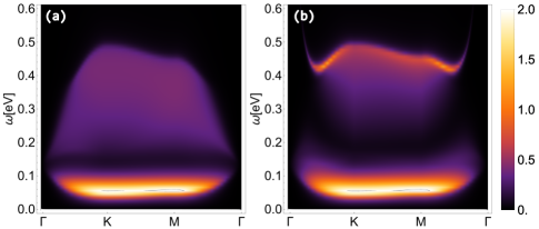
Figure 4: (a),(b) Spectral density of spinon susceptibility $\chi_{0/\mathrm{RPA}}$ in spinon Kondo lattice phase along high symmetry points without and with RPA correction.

Fig. 4 (a) and (b) depict the excitation spectrum of the spinon Kondo lattice phase, considering the bare and RPA susceptibilities, respectively. A low-energy branch of excitations is present, along with a continuum of particle-hole excitations at higher energies within the bare spectral density. The coupling between the parent quantum spin liquid and the Anderson impurity lattice is evidenced by a gap in the excitation spectrum. Fig. 4(b) presents the same excitation spectrum while incorporating the Coulomb interaction $V(\bm{q})$ through the RPA. The low-energy branch remains largely unaffected, but the upper continuum undergoes significant modifications due to the Coulomb interaction. Notably, the Coulomb interaction propels the magnetic excitations near the $\Gamma=(0,0)$ point to substantially higher energies.

IV.2 Internal energy and specific heat

We analyze the internal energy and specific heat of the spinon Kondo lattice phase using the bound-state electron Green’s function. For a U(1) quantum spin liquid with a spinon Fermi surface, the specific heat and thermal conductivity resemble those of a typical Fermi liquid; that is, they are proportional to the temperature at low temperatures [32, 33]. However, in our spinon Kondo lattice phase, the presence of the Anderson lattice leads to the formation of a spinon Kondo insulator, as depicted in Fig. 2(b), indicating that its internal energy and specific heat properties should differ.

The internal energy is calculated using the formula $U=\left\langle H\right\rangle=\int\omega D(\omega)n_{f}(\omega)d\omega$, where $D(\omega)$ is the spectral function. As discussed below Eq. (17), the electron density for the spinon Kondo lattice phase is $D_{\psi_{e}}(\omega)=-\frac{1}{\pi N}\sum_{\bm{q},\sigma,i,j}\mathrm{Im}\left[G(\psi_{e},\psi_{e}^{\dagger},\omega+i0^{+},\bm{q},\sigma)\right]_{ij}$. For comparison with a quantum spin liquid phase, we also consider the density of states of the latter phase as $D_{c}(\omega)=-\frac{1}{\pi N}\sum_{\bm{q},\sigma}\mathrm{Im}G(c,c^{\dagger},\omega+i0^{+},\bm{q},\sigma)$; for details see Appendix E. Here, $n_{f}(\omega)=\frac{1}{\exp\left(\beta\omega\right)+1}$ represents the Fermi distribution function. With these, the internal energy and specific heat can be calculated, and the results are shown in Fig. 5.

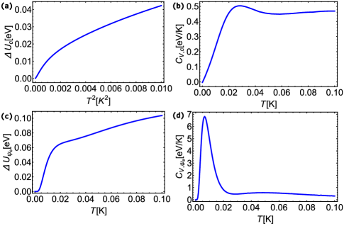
Figure 5: (a) Internal energy difference $\Delta U_{c}=U_{c}-U_{c,0}$ of electrons in QSL respect to temperature square $T^{2}$, where $U_{c}$ QSL electron internal energy and the $U_{c,0}$ is defined as the internal energy of QSL electron at $T=0\ \mathrm{K}$. (b) Temperature dependence of specific heat of QSL electron. (c) Internal energy difference $\Delta U_{\psi_{e}}$ of electron in spinon Kondo lattice phase respect to temperature $T$. $U_{\psi_{e}}$ and $U_{\psi_{e},0}$ are the electron internal in spinon Kondo lattice phase in arbitrary temperature and $T=0\ \mathrm{K}$ respectively. (d) Temperature dependence of electron specific heat in spinon Kondo lattice phase.

As demonstrated in Fig. 5(a), the internal energy of the pure spin liquid exhibits a linear relationship with the square of the temperature at low temperatures. This results in the specific heat being proportional to the temperature, as anticipated in the low-temperature regime approaching zero, as depicted in Fig. 5(b). In contrast, the electron specific heat of the spinon Kondo lattice phase remains invariant at low temperatures. This leads to a pronounced peak in the specific heat at low temperatures following a minimal zero plateau near $T=0\ \mathrm{K}$, indicative of insulator-like behavior.

V CONCLUSIONs

This work is primarily inspired by the recent experimental observations of the Kondo resonant state in cobalt atoms on a single-layer 1T-TaSe₂, which is a Mott insulator with a spin liquid ground state [16]. This phenomenon is akin to the Kondo effects observed in normal metals doped with dilute magnetic impurities. Theoretically, we consider a lattice of single-level quantum dots, the Anderson impurity lattice, which is coupled to a U(1) spin liquid with spinon Fermi surface. To address the Mott insulator and spin liquid phases, we employ the slave-rotor parton construction for both the Anderson lattice and the parent quantum spin liquid layer.

Let us briefly recapitulate the main findings and answers to questions posed in the introduction: (i) In the regime of strong Hubbard interaction across all lattice sites, including the parent triangular and Anderson impurity lattices, spinons persist as the sole low-energy degrees of freedom. Beyond a critical coupling between the parent triangular and Anderson impurity lattices leads to the hybridization of spinons across different layers, effectively dissolving localized spinons into the spinon Fermi surface of the spin liquid state. (ii) The interaction between the Anderson impurity lattice and the U(1) spin liquid gives rise to a novel phase, termed the spinon Kondo lattice phase. Hybridization of spinons from both lattices results in the formation of two spinon energy bands. Owing to half-filling of both lattices, the lower band is fully occupied and separated by a minor energy gap from the upper band, rendering the original spinon Fermi surface fully gapped and the hybridized phase a spinon Kondo insulator. (iii) The slave-rotor method inherently allows for an emergent local U(1) gauge symmetry. We investigated the influence of U(1) gauge fields by computing the bound state between spinons and chargons. Our many-body calculations indicate that bound state fluctuations do not significantly alter the spinon spectrum, only shifting high-energy states towards the proximate Mott band edges. (iv) Lastly, we examined the potential response of our model to neutron scattering measurements by assessing the magnetic susceptibility and to thermal measurements by evaluating the specific heat. Both measurements exhibit characteristics indicative of the spinon Kondo insulator phase.

Following up our work presented here, there are a few directions that we leave for future studies. In one front, one may consider the tunneling between the quantum dots and explore how it may affect the spinon Kondo lattice phase. This might parallel the spinon analogue of the FL^∗ phase. On another front, a natural extension of our study would be to consider broader classes of non-Abelian spin liquids with Fermi surfaces, such as the SU(2) spin liquid [8, 7, 34, 35], and their coupling to magnetic impurities. The presence of spinon pairing terms could lead to the discovery of various exotic topological quantum phases, including non-Abelian topological order, non-Abelian spinon metals, etc., which may serve as potential models for topological quantum computation [36, 37]. Thus, the spinon Kondo lattice phase characterized in this study presents potential theoretical and experimental framework for the investigation of novel phases.

Appendix A Derivation of the slave rotor Hamiltonian in canonical form

According to [9, 10], the Hamiltonian of the U(1) quantum spin liquid with Anderson impurity lattice can be represented using the slave rotor formalism. The Hamiltonian is given by:

$$H= \sum_{ij\sigma}t_{ij}c_{i,\sigma}^{\dagger}c_{j,\sigma}+\sum_{i\sigma}\epsilon_{d}d_{i,\sigma}^{\dagger}d_{i,\sigma}+V\sum_{i\sigma}c_{i,\sigma}^{\dagger}d_{i,\sigma}+h.c.+\frac{U_{QSL}}{2}\sum_{i}\left(\sum_{\sigma}c_{i,\sigma}^{\dagger}c_{i,\sigma}-1\right)^{2}+\frac{U}{2}\sum_{i}\left(\sum_{\sigma}d_{i,\sigma}^{\dagger}d_{i,\sigma}-1\right)^{2}$$

$$= \sum_{ij\sigma}t_{ij}f_{i,\sigma}^{\dagger}f_{j,\sigma}X_{j}^{\dagger}X_{i}+h.c.-\sum_{i\sigma}\left(\mu_{0}+h_{1,i}\right)f_{i,\sigma}^{\dagger}f_{i,\sigma}+\sum_{i\sigma}\left(\epsilon_{0}-h_{2}\right)a_{i,\sigma}^{\dagger}a_{i,\sigma}+V\sum_{i\sigma}f_{i,\sigma}^{\dagger}a_{i,\sigma}Y_{i}^{\dagger}X_{i}+h.c.$$

$$+\frac{U_{QSL}}{4}\sum_{i}L_{X,i}^{2}+\frac{U}{4}\sum_{i}L_{Y,i}^{2}.$$ (20)

To compute the angular momentum in the Hamiltonian, it is useful to first consider a two-dimensional rotor described by the coordinates $\left(x_{i},y_{i}\right)$ with the constraint $x_{i}^{2}+y_{i}^{2}=1$. The O(2) rotor is equivalent to the U(1) rotor, allowing the real space coordinates to be represented by complex numbers $X_{i}=x_{i}+iy_{i}$. The relationships between the coordinate operators, derivative operators, and momentum operators in real and complex coordinates are as follows:

$$\left(\begin{array}[]{c}x_{i}\\ y_{i}\end{array}\right)=\left(\begin{array}[]{cc}\frac{1}{2}&\frac{1}{2}\\ \frac{1}{2i}&-\frac{1}{2i}\end{array}\right)\left(\begin{array}[]{c}X_{i}\\ X_{i}^{\dagger}\end{array}\right), \frac{\partial}{\partial\left(\begin{array}[]{c}X_{i}\\ X_{i}^{\dagger}\end{array}\right)}=\left(\begin{array}[]{cc}\frac{1}{2}&\frac{1}{2i}\\ \frac{1}{2}&-\frac{1}{2i}\end{array}\right)\frac{\partial}{\partial\left(\begin{array}[]{c}x_{i}\\ y_{i}\end{array}\right)},$$ (33)

$$\frac{\partial}{\partial\left(\begin{array}[]{c}x_{i}\\ y_{i}\end{array}\right)}=\left(\begin{array}[]{cc}1&1\\ i&-i\end{array}\right)\frac{\partial}{\partial\left(\begin{array}[]{c}X_{i}\\ X_{i}^{\dagger}\end{array}\right)}, \left(\begin{array}[]{c}p_{x,i}\\ p_{y,i}\end{array}\right)=\left(\begin{array}[]{cc}1&1\\ i&-i\end{array}\right)\left(\begin{array}[]{c}P_{i}\\ P_{i}^{\dagger}\end{array}\right).$$ (46)

Additionally, the angular momentum operator in complex coordinate is:

$$L_{X,i}=x_{i}p_{y,i}-p_{x,i}y_{i}=i\left(X_{i}P_{i}-X_{i}^{\dagger}P_{i}^{\dagger}\right),$$ (47)

and the square of the angular momentum operator can be expressed in terms of the momentum operators:

$$L_{X,i}^{2}\rightarrow p_{x,i}^{2}+p_{y,i}^{2}=\left(P_{i}+P_{i}^{\dagger}\right)^{2}-\left(P_{i}-P_{i}^{\dagger}\right)^{2}=4P_{i}P_{i}^{\dagger}.$$ (48)

By incorporating these expressions similar ones for operator $L_{Y,i}$ into the original slave rotor Hamiltonian Eq. (20), we arrive at the final form of the slave rotor Hamiltonian Eq. (2). It is important to note that the coefficients $\frac{U}{2}$ and $\frac{U_{QSL}}{2}$ have been redefined as $\frac{U}{4}$ and $\frac{U_{QSL}}{4}$, respectively, to ensure the correct atomic limit, as pointed out in [9].

Appendix B Derivation of the self-consistent equations

To calculate the Green’s functions for spinons and chargons within the Hamiltonian denoted by Eqs. (3)-(5), we consider their respective equations of motion separately.

For the spinon Green’s function, the equation of motion is given by:

$$\left(\begin{array}[]{cc}i\omega_{n}-\epsilon_{0}&-w\\ -w&i\omega_{n}-h_{f}(\bm{k})\end{array}\right)\left(\begin{array}[]{c}G(a,a^{\dagger},\sigma,i\omega_{n})\\ G(f,a^{\dagger},i\omega_{n},\bm{k},\sigma)\end{array}\right)=\left(\begin{array}[]{c}1\\ 0\end{array}\right).$$ (49)

Solving these linear equations yields the Green’s functions for the spinon: Eqs. (11)-(13):

$$G(a,a^{\dagger},i\omega_{n},\sigma)=\frac{1}{i\omega_{n}-\epsilon_{d}-\frac{w^{2}}{i\omega_{n}-h_{f}(\bm{k})}},$$ (50)

$$G(f,a^{\dagger},i\omega_{n},\bm{k},\sigma)=\frac{wVG^{0}(f,f^{\dagger},i\omega_{n},\bm{k},\sigma)}{i\omega_{n}-\epsilon_{0}-w^{2}G^{0}(f,f^{\dagger},i\omega_{n},\bm{k},\sigma)}.$$ (51)

Similarly, For the chargon Green’s function, the equation of motion is:

$$\mathcal{G}^{-1}\left(i\nu_{n},\bm{k}\right)\left(\begin{array}[]{c}G\left(Y,Y^{\dagger},i\nu_{n},\bm{k}\right)\\ G\left(Q^{\dagger},Y^{\dagger},i\nu_{n},\bm{k}\right)\\ G\left(X,Y^{\dagger},i\nu_{n},\bm{k}\right)\\ G\left(P^{\dagger},Y^{\dagger},i\nu_{n},\bm{k}\right)\end{array}\right)=\left(\begin{array}[]{c}0\\ -i\\ 0\\ 0\end{array}\right),$$ (52)

where $\mathcal{G}^{-1}(i\nu_{n},\bm{k})$ is the inverse Green function of the chargon, expressed as:

$$\mathcal{G}^{-1}\left(i\nu_{n},\bm{k}\right)=i\nu_{n}\mathbf{1}_{4}-i\left(\begin{array}[]{cccc}0&U&0&0\\ -\lambda_{2}&0&u&0\\ 0&0&0&U_{QSL}\\ u&0&-\omega_{X}^{2}(\bm{k})&0\end{array}\right).$$ (53)

Following this method, one can derive the Green’s function expressions for the chargon, Eqs. (14)-(16):

$$G(Y,Y^{\dagger},i\nu_{n},\bm{k})=\frac{-1}{\frac{\nu_{n}^{2}}{U}+\lambda_{2}+u^{2}G^{0}(X,X^{\dagger},i\nu_{n},\bm{k})},$$ (54)

$$G(X,Y^{\dagger},i\nu_{n},\bm{k})=\frac{uG^{0}(X,X^{\dagger},i\omega_{n},k)}{\frac{\nu_{n}^{2}}{U}+\lambda_{2}+u^{2}G^{0}(X,X^{\dagger},i\nu_{n},\bm{k})},$$ (55)

$$G(X,X^{\dagger},i\nu_{n},\bm{k})=\frac{-1}{\frac{\nu_{n}^{2}}{U_{QSL}}+\omega_{X}^{2}(\bm{k})+u^{2}G^{0}(Y,Y^{\dagger},i\nu_{n},\bm{k})}.$$ (56)

According to the definitions of $u$ and $w$, and $\left\langle Y^{\dagger}Y\right\rangle=1$, we can obtain the Eqs. (6)-(8) in the main text.

Appendix C Translate chargon into canonical boson representation

Plug the expressions for $X_{k}=\frac{\sqrt{U_{QSL}}}{\sqrt{2\epsilon(k)}}\left(h_{k}+d_{k}^{\dagger}\right)$, $P_{k}=i\sqrt{\frac{\epsilon(k)}{2U_{QSL}}}\left(h_{k}^{\dagger}-d_{k}\right)$ into chargon part Hamiltonian in spin liquid:

$$H_{C}= \sum_{k}\omega^{2}_{X}(k)X_{k}^{\dagger}X_{k}+U_{QSL}\sum_{k}P_{k}^{\dagger}P_{k}$$

$$= \sum_{k}\frac{U_{QSL}\omega^{2}_{X}(k)}{2\epsilon(k)}\left(h_{k}^{\dagger}+d_{k}\right)\left(h_{k}+d_{k}^{\dagger}\right)+\sum_{k}\frac{\epsilon(k)}{2}\left(h_{k}-d_{k}^{\dagger}\right)\left(h_{k}^{\dagger}-d_{k}\right)$$

$$= \sum_{k}\frac{\epsilon(k)}{2}\left(h_{k}^{\dagger}h_{k}+h_{k}^{\dagger}d_{k}^{\dagger}+d_{k}h_{k}+d_{k}d_{k}^{\dagger}\right)+\sum_{k}\frac{\epsilon(k)}{2}\left(h_{k}h_{k}^{\dagger}-h_{k}d_{k}-d_{k}^{\dagger}h_{k}^{\dagger}+d_{k}^{\dagger}d_{k}\right)$$

$$= \sum_{k}\epsilon(k)\left(h_{k}^{\dagger}h_{k}+d_{k}^{\dagger}d_{k}+1\right).$$ (57)

In this equation, $\epsilon(k)=\sqrt{U_{QSL}}\omega_{X}(k)$ represents the chargon dispersion relation, and operators $h_{k}^{(\dagger)}$ and $d_{k}^{(\dagger)}$ are the annihilation (creation) operators for holons and doublons, respectively.

Appendix D Emergent U(1) gauge field in quantum spin liquid

In the context of quantum spin liquids, the slave rotor $X_{i}$ and its associated angular momentum $L_{i}$ can be interpreted as gauge fields, as discussed in seminal works by [38, 39, 40]. When the high-energy degrees of freedom for spinons and chargons are integrated out at the Gaussian level, a dynamic term for an emergent U(1) gauge field can be derived:

$$S_{G}= \frac{1}{g^{2}}\int_{0}^{\beta}d\tau\sum_{i}\mathrm{Re}\left[\prod_{\triangle}\exp\left(-iA_{\mu,i}a\right)\right].$$ (58)

Here, the gauge field $A_{\mu,i}$ arises from the Lagrange multiplier $h_{i}$ and local gauge redundancy. Furthermore, upon coarse-graining the lattice model, the continuum low-energy effective action for the U(1) quantum spin liquid with spinon Fermi surface is given by [24, 25, 17]:

$$S_{\mathrm{QSL}}=S_{S}+S_{C}+S_{M},$$ (59)

$$S_{S}=\int_{0}^{\beta}d\tau\int d\bm{r}\sum_{\sigma}\left[f_{\sigma,\bm{r}}^{\dagger}\left(\partial_{\tau}-iA_{0}(\bm{r})-\mu\right)f_{\sigma}(\bm{r})+\frac{\hbar^{2}}{2m_{f}}\left(\partial_{\bm{r}}+i\bm{A}(\bm{r})\right)f_{\sigma,\bm{r}}^{\dagger}\cdot\left(\partial_{\bm{r}}-i\bm{A}(\bm{r})\right)f_{\sigma}(\bm{r})\right],$$ (60)

$$S_{C}=\int_{0}^{\beta}d\tau\int d\bm{r}\left[\left(\partial_{\tau}+iA_{0}(\bm{r})\right)X^{\dagger}(\bm{r})\left(\partial_{\tau}-iA_{0}(\bm{r})\right)X(\bm{r})+\hbar^{2}v_{C}^{2}\left(\partial_{\bm{r}}+i\bm{A}(\bm{r})\right)X^{\dagger}(\bm{r})\left(\partial_{\bm{r}}-i\bm{A}(\bm{r})\right)X(\bm{r})+\Delta_{g}^{2}X^{\dagger}(\bm{r})X(\bm{r})\right],$$ (61)

$$S_{M}= \frac{1}{2g^{2}}\int_{0}^{\beta}d\tau\int d\bm{r}\left[\left(\nabla A_{0}(\bm{r})+\partial_{\tau}\bm{A}(\bm{r})\right)^{2}+\left(\nabla\times\bm{A}(\bm{r})\right)^{2}\right].$$ (62)

The coefficients above are as follows: $m_{f}$ represents the effective mass of the spinon, $v_{C}$ denotes the effective velocity of the chargon, and $g$ is the effective coupling constant. The magnitude of g is given by $g^{2}\sim\frac{\Delta_{g}^{2}}{tt_{F}}$ [6].

Utilizing the transformation of the chargon field $X_{\bm{r}}$ as outlined in the previous section Appendix B, we can derive the action for the chargon in the Schrödinger form:

$$S_{C}=\int_{0}^{\beta}\int d\bm{r}\left[h_{\bm{r}}^{\dagger}\left(\partial_{\tau}+iA_{0,\bm{r}}\right)h_{\bm{r}}+d_{\bm{r}}^{\dagger}\left(-\partial_{\tau}-iA_{0,\bm{r}}\right)d_{\bm{r}}+\epsilon(\partial_{\bm{r}}+i\bm{A}_{\bm{r}})h_{\bm{r}}^{\dagger}h_{\bm{r}}+\epsilon(\partial_{\bm{r}}+i\bm{A}_{\bm{r}})d_{\bm{r}}^{\dagger}d_{\bm{r}}\right],$$ (63)

where $\epsilon(\bm{k})=\sqrt{\hbar^{2}v_{C}^{2}\bm{k}^{2}+\Delta_{g}^{2}}$ is low energy limit of lattice version chargon dispersion.

In the vicinity of the Hubbard band edge energies, the group velocity exhibits diminutive values, resulting in the transverse component of gauge field fluctuations arising from the current-current correlation being negligible. Conversely, the dominant influence stems from the longitudinal component of gauge field fluctuations. Through the process of integrating out the gauge field $A_{0,\bm{r}}$, the interaction term between spinon, chargon and themselves can be derived:

$$S_{\textrm{int}}= \int_{0}^{\beta}d\tau\int d\bm{r}d\bm{r}^{\prime}V(\bm{r}-\bm{r}^{\prime})\sum_{\sigma,\sigma^{\prime}}\left[f_{\sigma,\bm{r}}^{\dagger}f_{\sigma,\bm{r}}f_{\sigma^{\prime},\bm{r}^{\prime}}^{\dagger}f_{\sigma^{\prime},\bm{r}^{\prime}}-\left(X_{\bm{r}}P_{\bm{r}}-X_{\bm{r}}^{\dagger}P_{\bm{r}}^{\dagger}\right)\left(X_{\bm{r}^{\prime}}P_{\bm{r}^{\prime}}-X_{\bm{r}^{\prime}}^{\dagger}P_{\bm{r}^{\prime}}^{\dagger}\right)+2if_{\sigma,\bm{r}}^{\dagger}f_{\sigma,\bm{r}}\left(X_{\bm{r}^{\prime}}P_{\bm{r}^{\prime}}-X_{\bm{r}^{\prime}}^{\dagger}P_{\bm{r}^{\prime}}^{\dagger}\right)\right]$$

$$= \int_{0}^{\beta}d\tau\int d\bm{r}d\bm{r}^{\prime}V(\bm{r}-\bm{r}^{\prime})\sum_{\sigma,\sigma^{\prime}}\left[f_{\sigma,\bm{r}}^{\dagger}f_{\sigma,\bm{r}}f_{\sigma^{\prime},\bm{r}^{\prime}}^{\dagger}f_{\sigma^{\prime},\bm{r}^{\prime}}+\left(a_{\bm{r}}^{\dagger}a_{\bm{r}}-b_{\bm{r}}^{\dagger}b_{\bm{r}}\right)\left(a_{\bm{r}^{\prime}}^{\dagger}a_{\bm{r}^{\prime}}-b_{\bm{r}^{\prime}}^{\dagger}b_{\bm{r}^{\prime}}\right)+2f_{\sigma,\bm{r}}^{\dagger}f_{\sigma,\bm{r}}\left(a_{\bm{r}^{\prime}}^{\dagger}a_{\bm{r}^{\prime}}-b_{\bm{r}^{\prime}}^{\dagger}b_{\bm{r}^{\prime}}\right)\right],$$ (64)

where Coulomb potential $V(\bm{r}-\bm{r}^{\prime})=\frac{g^{2}}{\left|\bm{r}-\bm{r}^{\prime}\right|}$.

Appendix E Calculate the Green’s function and density of states of the two-body bound state by Bethe-Salpeter equation

In the system considered in this article, the electron at position $\bm{r}_{i}$ is decomposed into spinon and chargon at the same lattice site, so when considering the two particles forming a bound state, we only need to analyze the coupling at the same location. Therefore, we start from the Bethe-Salpeter equation satisfied by two particles with same spatial coordinates:

$$G_{2}\left(4;1\right)= G_{1,0}\left(4,1\right)G_{1,0}\left(4,1\right)+\int dX_{c,2}dX_{c,3}G_{0}\left(4,3\right)G_{0}\left(4,3\right)K^{*}\left(3;2\right)G_{2}\left(2;1\right)$$ (65)

Here, $G_{2}$ is the the two-body Green’s function, and $G_{1,0}$ is the free single-particle Green’s function. $X_{c}=\frac{1}{2}(x_{1}+x_{2})$ represents the center coordinate. It is easily known that the system has a translation invariance, so $G_{2}\left(4;1\right)=G_{2}\left(X_{c,4}-X_{c,1}\right)$, which is independent of the relative coordinates, $\bar{x}=x_{1}-x_{2}$, and only depends on the difference of the center coordinates.

Upon transforming to the momentum space, we obtain:

$$\delta(P_{c,4}-P_{c,1})G_{2}\left(P_{c,1}\right)= \delta(P_{c,4}-P_{c,1})G_{0,p}\left(P_{c,1}\right)*G_{0,p}\left(P_{c,1}\right)+[\beta(2\pi)^{2}]^{-2}\int dP_{c,2}dP_{c,3}\delta(P_{c,4}-P_{c,3})G_{0,p}\left(P_{c,3}\right)*G_{0,p}\left(P_{c,3}\right)$$

$$\times\delta(P_{c,3}-P_{c,2})K_{p}^{*}\left(P_{c,2}\right)\delta(P_{c,2}-P_{c,1})G_{2}\left(P_{c,1}\right).$$ (66)

In this equation, the integral over the central momentum $P_{c}$ contains a sum over Matsubara frequencies. The Green’s functions in the expression are independent of the relative momentum $\bar{p}=\frac{1}{2}(p_{1}-p_{2})$, and it is easy to prove that the momentum of the spinon and chargons are equal in the system considered in this article.

For instance, in the case of the U(1) spin liquid with spinon Fermi surface on triangular lattice, we need to replace the Green’s functions in the above equation with those of the free spinons and chargons Eqs. (11)-(14), and substitute $G_{2}\left(P_{1}\right)=-G(c,c^{\dagger},i\omega_{n},\bm{k},\sigma)$.

Simultaneously, when analyzing the bound states of the spinons and charge carriers, it is necessary to consider the screen from the spinon Fermi sea. Here, we apply the Lindhard approximation, considering only the static RPA-corrected emergent Coulomb potential, $V_{s}(\bm{q})=V_{\mathrm{RPA}}(\omega=0,\bm{q})=\frac{g^{2}}{\bm{q}^{2}+\kappa^{2}}$, where $\kappa=g\sqrt{N_{f}}$ represents the Thomas-Fermi screening, and $N_{f}=D_{f}(0)$ is the density of states at the Fermi energy of the spinons.

Additionally, since we only consider interactions between on the same lattice site, the Yukawa potential could be further simplified to a local constant interaction [17]:

$$V_{\bm{r}}\approx\frac{g^{2}}{\left(2\pi\right)^{2}}\int\frac{1}{g^{2}N_{f}}d\bm{q}=\int\frac{d\bm{q}}{4\pi^{2}N_{f}}\approx\Lambda_{f},$$ (67)

where $\varLambda_{f}$ is the spinon half-bandwidth.

Therefore, the two-body kernel from local constant interaction can be concluded as a constant ladder approximation: $\frac{1}{(2\pi)^{2}}\int dkK^{*}\left(i\nu_{n},\bm{k}\right)\approx-\frac{i\nu_{n}V_{\bm{r}}}{U_{QSL}}$ [17]. Finally, we obtain the approximate Bethe-Salpeter equation for host spin liquid:

In the ladder approximation, the Bethe-Salpeter equation is given by [28, 29, 30]:

$$G(c,c^{\dagger},i\omega_{n},\bm{k}_{1},\sigma)= -\frac{1}{\beta N}\sum_{i\nu_{n},\bm{k}_{2}}G(f,f^{\dagger},i\omega_{n}+i\nu_{n},\bm{k}_{1}+\bm{k}_{2},\sigma)G(X,X^{\dagger},i\nu_{n},\bm{k}_{1})$$

$$-\frac{1}{\beta N}\sum_{i\nu_{n},\bm{k}_{2}}G(f,f^{\dagger},i\omega_{n}+i\nu_{n},\bm{k}_{1}+\bm{k}_{2},\sigma)G(X,X^{\dagger},i\nu_{n},\bm{k}_{1})$$

$$\times i\nu_{n}\frac{V_{\bm{r}}}{U_{QSL}}G(c,c^{\dagger},i\omega_{n},\bm{k}_{1},\sigma).$$ (68)

The simplified corrected electron Green’s function is shown as:

$$G(c,c^{\dagger},i\omega_{n},\bm{k}_{1},\sigma)= -\frac{1}{\beta N}\sum_{i\nu_{n},\bm{k}_{1}^{\prime}}G(f,f^{\dagger},i\omega_{n}+i\nu_{n},\bm{k}_{1}+\bm{k}_{1}^{\prime},\sigma)G(X,X^{\dagger},i\nu_{n},\bm{k}_{1}^{\prime})$$

$$\times\left[1-\frac{1}{\beta N}\sum_{i\nu_{n},\bm{k}_{1}^{\prime}}i\nu_{n}\frac{V_{\bm{r}}}{U_{QSL}}G(f,f^{\dagger},i\omega_{n}+i\nu_{n},\bm{k}_{1}+\bm{k}_{1}^{\prime},\sigma)G(X,X^{\dagger},i\nu_{n},\bm{k}_{1}^{\prime})\right]^{-1}$$ (69)

From this, the gauge field corrected electron spectral density can be obtained as $A_{\mathrm{QSL}}(\omega,\bm{k}_{1})=-\frac{1}{\pi}\mathrm{Im}G(c,c^{\dagger},\omega+i0^{+},\bm{k}_{1},\sigma)$, and its spectral function $D_{\mathrm{QSL}}(\omega)=\frac{1}{N}\sum_{\bm{k}_{1}}A_{\mathrm{QSL}}(\omega,\bm{k}_{1})$, as shown in Fig. 6.

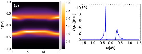
Figure 6: (a) QSL bound state electron spectral density $A_{\mathrm{QSL}}(\omega,\bm{k})$ along high symmetry points. (b) QSL bound state electron spectral function $D_{\mathrm{QSL}}(\omega)$. Both (a) and (b) are under local interaction strength $V_{r}=0.225\ \mathrm{eV}$.

In terms of QSL with Anderson lattice, by substituting the complete spinon and chargon Green’s functions into Eq. (66), and define $G_{2}\left(P_{1}\right)=-G(\psi_{e},\psi_{e}^{\dagger},i\omega_{n},\bm{k},\sigma)$, we can obtain the Eq. (17) discussed earlier.

Those full Green’s functions in Eq. (66) are:

$$G^{-1}(\psi_{s},\psi_{s}^{\dagger},i\omega_{n},\bm{k},\sigma)=\left(\begin{array}[]{cc}G_{0}^{-1}(a,a^{\dagger},i\omega_{n},\sigma)&-w\\ -w&G_{0}^{-1}(f,f^{\dagger},i\omega_{n},\bm{k},\sigma)\end{array}\right),$$ (70)

$$G^{-1}(Z_{c},Z_{c}^{\dagger},i\nu_{n},k)=\left(\begin{array}[]{cc}G_{0}^{-1}(Y,Y^{\dagger},i\nu_{n})&u\\ u&G_{0}^{-1}(X,X^{\dagger},i\nu_{n},\bm{k})\end{array}\right).$$ (71)

Similar to Eq. (68), the expression for the electron Green’s function in the QSLAL can be readily obtained:

$$G(\psi_{e},\psi_{e}^{\dagger},i\omega_{n},\bm{k}_{1},\sigma)= -\frac{1}{\beta N}\sum_{i\nu_{n},\bm{k}_{2}}G(\psi_{s},\psi_{s}^{\dagger},i\omega_{n}+i\nu_{n},\bm{k}_{1}+\bm{k}_{2},\sigma)\otimes G(Z_{c},Z_{c}^{\dagger},i\nu_{n},\bm{k}_{1})$$

$$-\frac{1}{\beta N}\sum_{i\nu_{n},\bm{k}_{2}}G(\psi_{s},\psi_{s}^{\dagger},i\omega_{n}+i\nu_{n},\bm{k}_{1}+\bm{k}_{2},\sigma)\otimes G(Z_{c},Z_{c}^{\dagger},i\nu_{n},\bm{k}_{1})$$

$$\times i\nu_{n}\frac{V_{\bm{r}}}{U_{QSL}}G(\psi_{e},\psi_{e}^{\dagger},i\omega_{n},\bm{k}_{1},\sigma).$$ (72)

As an analogy of Eq. (68) The simplified corrected electron Green’s function for QSLAL is given in Eq. (17)

and their spectral function $A_{\mathrm{AL/QSL}}(\omega,\bm{k}_{1})$ are shown in Fig. 7.

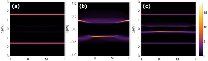
Figure 7: (a), (b), (c) are spectral density of electron in spinon Kondo lattice phase along the high symmetry points for Anderson lattice part, host spin liquid part and the whole system together respectively, all with the interaction strength $V_{\bm{r}}=0.225\ \mathrm{eV}$.

References

- Anderson [1973] P. Anderson, Materials Research Bulletin 8, 153 (1973).
- Anderson [1987] P. W. Anderson, Science 235, 1196 (1987).
- Wen [2002] X.-G. Wen, Phys. Rev. B 65, 165113 (2002).
- Wen [2004] X. Wen, Quantum Field Theory of Many-Body Systems: From the Origin of Sound to an Origin of Light and Electrons, Oxford Graduate Texts (OUP Oxford, 2004).
- Chen et al. [2010] X. Chen, Z.-C. Gu, and X.-G. Wen, Phys. Rev. B 82, 155138 (2010).
- Lee and Lee [2005] S.-S. Lee and P. A. Lee, Phys. Rev. Lett. 95, 036403 (2005).
- Lee et al. [2006] P. A. Lee, N. Nagaosa, and X.-G. Wen, Rev. Mod. Phys. 78, 17 (2006).
- Lee et al. [1998] P. A. Lee, N. Nagaosa, T.-K. Ng, and X.-G. Wen, Phys. Rev. B 57, 6003 (1998).
- Florens and Georges [2002] S. Florens and A. Georges, Phys. Rev. B 66, 165111 (2002).
- Florens and Georges [2004] S. Florens and A. Georges, Phys. Rev. B 70, 035114 (2004).
- Swingle [2010] B. Swingle, Phys. Rev. Lett. 105, 050502 (2010).
- Zhang et al. [2011] Y. Zhang, T. Grover, and A. Vishwanath, Phys. Rev. Lett. 107, 067202 (2011).
- Anderson [1961] P. W. Anderson, Phys. Rev. 124, 41 (1961).
- Kondo [1964] J. Kondo, Progress of Theoretical Physics 32, 37 (1964).
- Hewson [1997] A. Hewson, The Kondo Problem to Heavy Fermions, Cambridge Studies in Magnetism (Cambridge University Press, 1997).
- Chen et al. [2022] Y. Chen, W.-Y. He, W. Ruan, J. Hwang, S. Tang, R. L. Lee, M. Wu, T. Zhu, C. Zhang, H. Ryu, F. Wang, S. G. Louie, Z.-X. Shen, S.-K. Mo, P. A. Lee, and M. F. Crommie, Nature Physics 18, 1335 (2022).
- He and Lee [2022] W.-Y. He and P. A. Lee, Phys. Rev. B 105, 195156 (2022).
- Coleman et al. [2005] P. Coleman, J. B. Marston, and A. J. Schofield, Phys. Rev. B 72, 245111 (2005).
- Coleman [1983] P. Coleman, Phys. Rev. B 28, 5255 (1983).
- Coleman [2015] P. Coleman, Introduction to Many-Body Physics (Cambridge University Press, 2015).
- Burdin et al. [2002] S. Burdin, D. R. Grempel, and A. Georges, Phys. Rev. B 66, 045111 (2002).
- Senthil et al. [2004] T. Senthil, M. Vojta, and S. Sachdev, Phys. Rev. B 69, 035111 (2004).
- Sachdev [2023] S. Sachdev, Quantum Phases of Matter (Cambridge University Press, 2023).
- Senthil [2008] T. Senthil, Phys. Rev. B 78, 045109 (2008).
- Podolsky et al. [2009] D. Podolsky, A. Paramekanti, Y. B. Kim, and T. Senthil, Phys. Rev. Lett. 102, 186401 (2009).
- Hermele et al. [2004] M. Hermele, T. Senthil, M. P. A. Fisher, P. A. Lee, N. Nagaosa, and X.-G. Wen, Phys. Rev. B 70, 214437 (2004).
- Lee [2009] S.-S. Lee, Phys. Rev. B 80, 165102 (2009).
- Salpeter and Bethe [1951] E. E. Salpeter and H. A. Bethe, Phys. Rev. 84, 1232 (1951).
- Greiner and Reinhardt [2003] W. Greiner and J. Reinhardt, Quantum Electrodynamics, Physics and astronomy online library (Springer, 2003).
- Lurie [1968] D. Lurie, Particles and Fields (Interscience Publishers, 1968).
- Banerjee et al. [2016] A. Banerjee, C. A. Bridges, J.-Q. Yan, A. A. Aczel, L. Li, M. B. Stone, G. E. Granroth, M. D. Lumsden, Y. Yiu, J. Knolle, S. Bhattacharjee, D. L. Kovrizhin, R. Moessner, D. A. Tennant, D. G. Mandrus, and S. E. Nagler, Nature Materials 15, 733 (2016).
- Ribak et al. [2017] A. Ribak, I. Silber, C. Baines, K. Chashka, Z. Salman, Y. Dagan, and A. Kanigel, Phys. Rev. B 96, 195131 (2017).
- Murayama et al. [2020] H. Murayama, Y. Sato, T. Taniguchi, R. Kurihara, X. Z. Xing, W. Huang, S. Kasahara, Y. Kasahara, I. Kimchi, M. Yoshida, Y. Iwasa, Y. Mizukami, T. Shibauchi, M. Konczykowski, and Y. Matsuda, Phys. Rev. Res. 2, 013099 (2020).
- Hermele [2007] M. Hermele, Phys. Rev. B 76, 035125 (2007).
- Chen et al. [2012] G. Chen, A. Essin, and M. Hermele, Phys. Rev. B 85, 094418 (2012).
- Kitaev [2003] A. Kitaev, Annals of Physics 303, 2 (2003).
- Nayak et al. [2008] C. Nayak, S. H. Simon, A. Stern, M. Freedman, and S. Das Sarma, Rev. Mod. Phys. 80, 1083 (2008).
- Senthil and Fisher [2000] T. Senthil and M. P. A. Fisher, Phys. Rev. B 62, 7850 (2000).
- Qi and Sachdev [2010] Y. Qi and S. Sachdev, Phys. Rev. B 81, 115129 (2010).
- Sachdev [2018] S. Sachdev, Reports on Progress in Physics 82, 014001 (2018).