Stabilization of a Class of Large-Scale Systems of Linear Hyperbolic PDEs via Continuum Approximation of Exact Backstepping Kernels^∗

Abstract

We establish that stabilization of a class of linear, hyperbolic partial differential equations (PDEs) with a large (nevertheless finite) number of components, can be achieved via employment of a backstepping-based control law, which is constructed for stabilization of a continuum version (i.e., as the number of components tends to infinity) of the PDE system. This is achieved by proving that the exact backstepping kernels, constructed for stabilization of the large-scale system, can be approximated (in certain sense such that exponential stability is preserved) by the backstepping kernels constructed for stabilization of a continuum version (essentially an infinite ensemble) of the original PDE system. The proof relies on construction of a convergent sequence of backstepping kernels that is defined such that each kernel matches the exact backstepping kernels (derived based on the original, large-scale system), in a piecewise constant manner with respect to an ensemble variable; while showing that they satisfy the continuum backstepping kernel equations. We present a numerical example that reveals that complexity of computation of stabilizing backstepping kernels may not scale with the number of components of the PDE state, when the kernels are constructed on the basis of the continuum version, in contrast to the case in which they are constructed on the basis of the original, large-scale system. In addition, we formally establish the connection between the solutions to the large-scale system and its continuum counterpart. Thus, this approach can be useful for design of computationally tractable, stabilizing backstepping-based control laws for large-scale PDE systems.

Backstepping control, hyperbolic PDEs, large-scale systems, PDE continua.

1 Introduction

1.1 Motivation

Large-scale systems of 1-D hyperbolic PDEs appear in a variety of applications involving transport phenomena and which incorporate different, interconnected components. Among them, large-scale interconnected hyperbolic systems may be used to describe the dynamics of blood flow, from the location of the heart all the way through to points where non-invasive measurements can be obtained [1], [2], of epidemics spreading, to describe transport of epidemics among different geographical regions [3], and of traffic flows, to model density and speed dynamics in interconnected highway segments [4, 5] and in urban networks [6], to name a few [7]. Backstepping is a systematic design approach to construction of explicit feedback laws for general classes of such systems [8, 9, 10, 11, 12, 13, 14]. Due to potentially large number of interacting components, incorporated in such systems, computational complexity of exact backstepping-based control designs may increase significantly, in a manner proportional with the number of state components. Motivated by this, in the present paper we aim at developing an approach to computing backstepping kernels for large-scale hyperbolic PDE systems, such that computational complexity remains tractable, even when the number of state components becomes very large, while at the same time, provably retaining the stability guarantees of backstepping. We achieve this via approximating the exact backstepping kernels, computed based on a large number of PDEs, utilizing a single kernel that is derived based on a continuum version of the exact kernels PDEs, and capitalizing on the robustness properties of backstepping for the class of systems considered, to additive control gain errors.

1.2 Literature

The approach of design of feedback laws for large-scale systems based on a continuum version of the system considered has been utilized for large-scale ordinary differential equation (ODE) systems, such as, for example, in [16, 17, 18, 19, 20, 21, 22, 23]. However, such an approach has not been utilized so far for large-scale systems whose state components are PDEs. The main goals of the approach developed here, may be viewed also as related to control design approaches that aim at providing computational means towards implementation of PDE backstepping-based control laws with provable stability guarantees, such as, for example, neural operators-based [24], late-lumping-based [25], and power series-based [26], backstepping control laws. Our approach may be viewed as complementary and different from these results, in that the main goal is to address complexity due to a potential radical increase in the number of state components, instead of complexity of actual numerical implementation (even though these existing results can be combined with the approach presented here, for numerical implementation of the controllers).

1.3 Contributions

In the present paper, we provide backstepping-based feedback laws for a class of large-scale systems of 1-D hyperbolic PDEs, which are described by the class of systems considered in [13], when the number of state components $n$ is large. The key idea of our approach is to construct approximate backstepping kernels for stabilization of the large-scale (nevertheless, with a finite number of components) system relying on the continuum backstepping kernels developed in [27] for a continuum version of the original, large-scale system. We establish stability of the closed-loop system consisting of the original, large-scale PDE system under a backstepping-based feedback law that employs the approximate kernels, constructed based on the continuum version of the PDE system. The stability proof consists of three main steps.

In the first, we construct a sequence of backstepping kernels that is defined such that each kernel matches with the exact backstepping kernel (derived based on the original, large-scale system) in a piecewise constant manner with respect to an ensemble variable; while showing that the kernels in the sequence satisfy the continuum kernel equation. For the proof we rely on a transformation that maps functions (the exact backstepping kernels) on a 2-D domain, to functions (the approximate kernels derived based on the continuum) on a 3-D domain in a piecewise constant manner in $L^{2}$ sense. In the second step, we show that this sequence converges to the continuum backstepping kernel, obtained from a direct application of backstepping to a continuum version of the large-scale system. For the proof we rely on the well-posedness of the backstepping kernels (both the continuum and exact kernels) and density arguments. In the third step, we establish stability of the closed-loop system employing an abstract systems framework. For the proof we recast the closed-loop system’s dynamics as perturbed dynamics of the nominal (based on employment of the exact kernels) closed-loop system, showing that the size of the perturbation, due to the additive error that originates from the approximation error of the exact stabilizing control gains, can be made arbitrarily small (in $L^{2}$) for sufficiently large $n$.

We also provide an alternative stability proof employing a Lyapunov functional, which allows quantification of overshoot and decay rate of the closed-loop system’s response. Furthermore, for enabling generalization of the approach introduced, for computation of stabilizing control gains based on continuum approximations, to other classes of large-scale PDE systems, we also establish the formal connection between the solutions to the original $n+1$ system and the solutions to its continuum counterpart. In particular, we show that when the number of state components is sufficiently large, the solutions to the large-scale system can be approximated by the solutions to the continuum system, provided that the data (i.e., parameters, initial conditions, and inputs) of the $n+1$ PDE problem can be approximated by the respective data of the continuum PDE problem. The proof relies on construction of a sequence of solutions, obtained in a piecewise constant manner (with respect to an ensemble variable) from the solutions to the $n+1$ system, which is subsequently shown (via utilization of the well-posedness property of the continuum that we prove) to converge to the solution of the continuum system.

We then present a numerical example that illustrates that computation of (approximate) stabilizing kernels based on the continuum kernel may provide flexibility in computation, as well as it may significantly improve computational complexity. In particular, in this specific example, although computation of the exact backstepping kernels may require to solve implicitly the corresponding $n+1$ hyperbolic kernels PDEs, as closed-form solutions may not be available, the approximate kernels can be computed with only algebraic computations, since the continuum kernel is available in closed form. We also present respective simulation investigations, which validate the theoretical developments, showing that as the number of components of the large-scale system increases the performance of the closed-loop systems, under the approximate control laws, is improved. In particular, we illustrate that the approximate control kernels converge to the exact kernels, and thus, as $n$ increases, the performance of the closed-loop system becomes similar to the performance under the exact control gain kernels.

1.4 Organization

We start in Sections 2 and 3 presenting both the large-scale PDE system and its continuum counterpart, together with the respective exact and continuum backstepping kernels PDEs. In Section 4 we establish stability of the large-scale, closed-loop system under the approximate control law. In Section 5 we present a numerical example and consistent simulation results. In Section 6 we study the connection between the solutions to the large-scale system and its continuum counterpart. In Section 7 we discuss separately the case $n\to\infty$. In Section 8 we provide concluding remarks and discuss related topics of our current research.

1.5 Notation

We use the standard notation $L^{2}(\Omega;\mathbb{R})$ for real-valued Lebesque integrable functions on a domain $\Omega$, and on one dimensional domains $H^{1}$ denotes the corresponding Sobolev space. Similarly, $L^{\infty}(\Omega;\mathbb{R}),C(\Omega;\mathbb{R}),C^{1}(\Omega;\mathbb{R})$ denote essentially bounded, continuous, and continuously differentiable functions, respectively, on $\Omega$. Moreover, $f\in L_{\rm{loc}}^{2}([0,+\infty);\mathbb{R})$ means that $f\in L^{2}([0,m];\mathbb{R})$ for any $m\in\mathbb{N}$. We denote vectors and matrices by bold symbols, and $\|\cdot\|_{\infty}$ denotes the maximum absolute row sum of a matrix (or a vector). For any $n\in\mathbb{N}$, we denote by $E$ the Hilbert space $L^{2}([0,1];\mathbb{R}^{n+1})$ equipped with the inner product

$$\left\langle\left(\begin{smallmatrix}\mathbf{u}_{1}\\ v_{1}\end{smallmatrix}\right),\left(\begin{smallmatrix}\mathbf{u}_{2}\\ v_{2}\end{smallmatrix}\right)\right\rangle_{E}=\int\limits_{0}^{1}\left(\frac{1}{n}\sum_{i=1}^{n}u_{1}^{i}(x)u_{2}^{i}(x)+v_{1}(x)v_{2}(x)\right)dx,$$ (1)

which induces the norm $\left\|\cdot\right\|_{E}=\sqrt{\left<\cdot,\cdot\right>_{E}}$. We also define the continuum version of $E$ as $E_{c}=L^{2}([0,1];L^{2}([0,1];\mathbb{R}))\times L^{2}([0,1];\mathbb{R})$, (i.e., $\mathbb{R}^{n}$ becomes $L^{2}([0,1];\mathbb{R})$ as $n\to\infty$) equipped with the inner product

$$\left\langle\left(\begin{smallmatrix}u_{1}\\ v_{1}\end{smallmatrix}\right),\left(\begin{smallmatrix}u_{2}\\ v_{2}\end{smallmatrix}\right)\right\rangle_{E_{c}} =$$

$$\int\limits_{0}^{1}\left(\int\limits_{0}^{1}u_{1}(x,y)u_{2}(x,y)dy+v_{1}(x)v_{2}(x)\right)dx,$$ (2)

which coincides with $L^{2}([0,1]^{2};\mathbb{R})\times L^{2}([0,1];\mathbb{R})$. Moreover, $\mathcal{L}(E,\mathbb{R})$ denotes the space of bounded linear operators from $E$ to $\mathbb{R}$, and $\|\cdot\|_{\mathcal{L}(E,\mathbb{R})}$ is the corresponding operator norm. For $\mathcal{L}(E,E)$, we denote $\mathcal{L}(E)$. Finally, we say that a system is exponentially stable (on $E$; resp. on $E_{c}$) if for any initial condition $z_{0}\in E$ (resp. $z_{0}\in E_{c}$) the (weak) solution $z(t)$ of the system satisfies $\|z(t)\|_{E}\leq Me^{-ct}\|z_{0}\|_{E}$ (resp. $\|z(t)\|_{E_{c}}\leq Me^{-ct}\|z_{0}\|_{E_{c}}$) for some $M,c>0$.

2 Stabilization of Large-Scale Systems of Linear Hyperbolic PDEs via Exact Backstepping Kernels

For $n\geq 1$ consider the following set of $n+1$ transport PDEs on $x\in[0,1]$ for $i=1,\ldots,n$

$$u_{t}^{i}(t,x)+\lambda_{i}(x)u_{x}^{i}(t,x) =\frac{1}{n}\sum_{j=1}^{n}\sigma_{i,j}(x)u^{j}(t,x)$$

$$\quad+W_{i}(x)v(t,x),$$ (3a)

$$v_{t}(t,x)-\mu(x)v_{x}(t,x) =\frac{1}{n}\sum_{j=1}^{n}\theta_{j}(x)u^{j}(t,x),$$ (3b)

with boundary conditions

$$u^{i}(t,0)=q_{i}v(t,0),\qquad v(t,1)=U(t),$$ (4)

where $U\in L_{\rm{loc}}^{2}([0,+\infty);\mathbb{R})$ is the control input. The initial conditions of (3) are $u^{i}(0,x)=u^{i}_{0}(x),v(0,x)=v_{0}(x)$, where $u_{0}^{i},v_{0}\in L^{2}([0,1];\mathbb{R})$. The parameters of the system (3), (4) satisfy the following assumption.

Assumption 2.1

We assume that $\mu,\lambda_{i}\in C^{1}([0,1];\mathbb{R})$, $\sigma_{i,j},W_{i},\theta_{i}\in C([0,1];\mathbb{R})$ and $q_{i}\in\mathbb{R}$ for all $i,j=1,2,\dots,n$. Moreover, the transport velocities are assumed to satisfy $-\mu(x)<0<\lambda_{i}(x)$, for all $x\in[0,1]$ and $i=1,2,\ldots,n$.

Remark 2.2

The presentation of the system (3), (4) is motivated from [13]. However, here we also make the following modifications. Most notably, the factor $1/n$ appears in (3). This is equivalent to equipping the $n$-part of the system with the scaled inner product $n^{-1}\langle\cdot,\cdot\rangle_{\mathbb{R}^{n}}$. With the scaling, we guarantee that the sums remain bounded and convergent as $n\to\infty$ without having to pose any additional constraints on the parameters of (3), (4). If one wishes to proceed without scaling the sums, then some additional assumptions are needed, e.g., that the respective parameters form $\ell^{p}$ sequences for some $p\in[1,+\infty]$, such that the sums are well-defined as $n\to\infty$. The other noteworthy modification has to do with Assumption 2.1. In [13], the transport velocities are assumed to satisfy $-\mu(x)<0<\lambda_{1}(x)<\lambda_{2}(x)<\ldots<\lambda_{n}(x),\forall x\in[0,1]$ to guarantee strict hyperbolicity and well-posedness of (3), (4). Nevertheless, well-posedness can be guaranteed under Assumption 2.1, e.g., based on [30, Sect. 13.2] as we show in Proposition .1.1 in Appendix .1. Due to well-posedness, the system (3), (4) has a well-defined, unique, weak solution $\left(\left(u^{i}(t,x)\right)_{i=1}^{n},v(t,x)\right)$ on $E$, where $u^{i},v\in C([0,+\infty);L^{2}([0,1];\mathbb{R}))$ [31, Prop. 4.2.5, Rem. 4.1.2].

It follows from [13, Thm 3.2] that the system (3), (4) is exponentially stabilizable by a state feedback law of the form

$$U(t)=\int\limits_{0}^{1}\left[\frac{1}{n}\sum_{i=1}^{n}k^{i}(1,\xi)u^{i}(t,\xi)+k^{n+1}(1,\xi)v(t,\xi)\right]d\xi,$$ (5)

where, for $i=1,\ldots,n+1$, $k^{i}$ satisfy

$$\mu(x)k_{x}^{i}(x,\xi)-\lambda_{i}(\xi)k_{\xi}^{i}(x,\xi) =$$

$$\lambda_{i}^{\prime}(\xi)k^{i}(x,\xi)+\frac{1}{n}\sum_{j=1}^{n}\sigma_{j,i}(\xi)k^{j}(x,\xi)+\theta_{i}(\xi)k^{n+1}(x,\xi),$$ (6a)

$$\mu(x)k_{x}^{n+1}(x,\xi)+\mu(\xi)k_{\xi}^{n+1}(x,\xi) =$$

$$-\mu^{\prime}(\xi)k^{n+1}(x,\xi)+\frac{1}{n}\sum_{j=1}^{n}W_{j}(\xi)k^{j}(x,\xi),$$ (6b)

on a triangular domain $0\leq\xi\leq x\leq 1$ with boundary conditions

$$k^{i}(x,x) =-\frac{\theta_{i}(x)}{\lambda_{i}(x)+\mu(x)},$$ (7a)

$$\mu(0)k^{n+1}(x,0) =\frac{1}{n}\sum_{j=1}^{n}q_{j}\lambda_{j}(0)k^{j}(x,0),$$ (7b)

for all $x\in[0,1]$. Note the scaling of the sums by $1/n$ as per Remark 2.

3 Stabilization of a Continuum of Linear Hyperbolic PDEs via Continuum Backstepping

While large-scale, yet, consisting of a finite-number of components, systems of hyperbolic PDEs can be studied in the framework of Section 2, we also consider the continuum limit case as $n\to\infty$, for which we present the generic framework of a continuum of hyperbolic PDEs studied in [27] and sketched in Fig. 1. That is, instead of having $n$ rightward transport PDEs as in Section 2, consider a continuum of such PDEs as in [27] with $y\in[0,1]$ being the index variable

$$u_{t}(t,x,y)+\lambda(x,y)u_{x}(t,x,y) =\int\limits_{0}^{1}\sigma(x,y,\eta)u(t,x,\eta)d\eta$$

$$\quad+W(x,y)v(t,x),$$ (8a)

$$v_{t}(t,x)-\mu(x)v_{x}(t,x) =\int\limits_{0}^{1}\theta(x,y)u(t,x,y)dy,$$ (8b)

with boundary conditions

$$u(t,0,y)=q(y)v(t,0),\qquad v(t,1)=U(t),$$ (9)

for almost every $y\in [0,1]$, i.e., the continuum variables and parameters are considered $L^{2}([0,1];\mathbb{R})$ functions in $y$. The following assumption is needed, for the parameters involved in (8), (9), to guarantee the existence of a continuum backstepping control law [27, Thm 3].

Assumption 3.1

We assume that $\mu\in C^{1}([0,1];\mathbb{R}),\lambda\in C^{1}\left([0,1]^{2};\mathbb{R}\right),W,\theta\in C([0,1];L^{2}([0,1];\mathbb{R})),\sigma\in C\left([0,1];L^{2}([0,1]^{2};\mathbb{R})\right)$, and $q\in C([0,1];\mathbb{R})$. Moreover, $\lambda(x,y)>0$ uniformly for all $x\in[0,1]$ and almost every $y\in[0,1]$, and $-\mu(x)<0$ for all $x\in[0,1]$.

Figure 1: Schematic view of the continuum PDE system (8), (9). Boundary terms are denoted in magenta and in-domain terms are denoted in blue.

By [27, Thm 1], the system (8), (9) is exponentially stabilizable by a state feedback law of the form

$$U(t)=\int\limits_{0}^{1}\left[\int\limits_{0}^{1}k(1,\xi,y)u(t,\xi,y)dy+\bar{k}(1,\xi)v(t,\xi)\right]d\xi,$$ (10)

where $k,\bar{k}$ satisfy

$$\mu(x)k_{x}(x,\xi,y)-\lambda(\xi,y)k_{\xi}(x,\xi,y)-\theta(\xi,y)\bar{k}(x,\xi) =$$

$$\lambda_{\xi}(\xi,y)k(x,\xi,y)+\int\limits_{0}^{1}\sigma(\xi,\eta,y)k(x,\xi,\eta)d\eta,$$ (11a)

$$\mu(x)\bar{k}_{x}(x,\xi)+\mu(\xi)\bar{k}_{\xi}(x,\xi) =$$

$$-\mu^{\prime}(\xi)\bar{k}(x,\xi)+\int\limits_{0}^{1}W(\xi,y)k(x,\xi,y)dy,$$ (11b)

on a triangular domain $0\leq\xi\leq x\leq 1$ with boundary conditions

$$k(x,x,y) =-\frac{\theta(x,y)}{\lambda(x,y)+\mu(x)},$$ (12a)

$$\mu(0)\bar{k}(x,0) =\int\limits_{0}^{1}q(y)\lambda(0,y)k(x,0,y)dy,$$ (12b)

for almost every $y\in[0,1]$.

4 Stabilization of the Finite Large-Scale System via Continuum Approximation of Exact Kernels

4.1 Statement of the Main Result

The core idea of the continuum approximation that we present here is that we approximate $n+1$ kernel equations by a continuum of kernel equations. Provided that the approximation is sufficiently accurate, we show that the backstepping controller derived from the continuum kernel equations exponentially stabilizes the $n+1$ system associated with the original finite system of $n+1$ PDEs.

Thus, consider an $n+1$ system (3), (4) with parameters $\lambda_{i},W_{i},\theta_{i},\sigma_{i,j},q_{i}$ for $i,j=1,2,\ldots,n$ satisfying Assumption 2.1 and consider any continuous functions $\lambda,W,\theta,\sigma,q$ that satisfy Assumption 3.1 with

$$\lambda(x,i/n) =\lambda_{i}(x),$$ (13a)

$$W(x,i/n) =W_{i}(x),$$ (13b)

$$\theta(x,i/n) =\theta_{i}(x),$$ (13c)

$$\sigma(x,i/n,j/n) =\sigma_{i,j}(x),$$ (13d)

$$q(i/n) =q_{i},$$ (13e)

for all $x\in[0,1]$ and $i,j=1,2,\ldots,n$. There are infinitely many functions satisfying (13) and Assumption 3.1, as well as ways to construct them, e.g., by utilizing auxiliary functions $\left\{p_{i}\right\}_{i=1}^{n}$ that satisfy $p_{i}(i/n)=1$ and $p_{\ell}(i/n)=0$ for $\ell\neq i$. The relations in (13) could as well be defined in other ways, e.g., using $(i-1)/n$ in place of $i/n$, but we find (13) the most convenient option for our developments. The continuum kernel equations (11), (12) with parameters $\lambda,\mu,W,\theta,\sigma,q$, satisfying (13) and Assumption 3.1 have a unique, continuous solution $(k,\bar{k})$ by [27, Thm 3]. Thus, construct the following functions for all $0\leq\xi\leq x\leq 1$

$$\widetilde{k}^{i}(x,\xi) =k(x,\xi,i/n),\quad i=1,2,\ldots,n,$$ (15a)

$$\widetilde{k}^{n+1}(x,\xi) =\bar{k}(x,\xi).$$ (15b)

Our main result is the following.

Theorem 4.1

Consider an $n+1$ system (3), (4) with parameters $\lambda_{i},\mu,W_{i},\theta_{i},\sigma_{i,j},q$ for $i,j=1,2,\ldots,n$ satisfying Assumption 2.1. Let the parameters $\lambda,\mu,W,\theta,\sigma,q$ satisfy Assumption 3.1 and relations (13). Then

$$U(t) =\int\limits_{0}^{1}\left[\frac{1}{n}\sum_{i=1}^{n}\widetilde{k}^{i}(1,\xi)u^{i}(t,\xi)+\widetilde{k}^{n+1}(1,\xi)v(t,\xi)\right]d\xi,$$ (16)

where $\left(\widetilde{k}^{i}\right)_{i=1}^{n+1}$ are given in (15), with $\left(k,\bar{k}\right)$ being the solution to (11), (12), exponentially stabilizes system (3), (4).

4.2 Proof of Theorem 4.1

The proof of Theorem 4.1 relies on Lemmas 4.2 and 4.4 presented below. We show first that the functions defined in (15) approximate the solutions to the $n+1$ kernel equations (6), (7) to arbitrary accuracy as $n$ increases. In order to do this, we first interpret the solutions to the $n+1$ kernels equations (6), (7) as piecewise constant solutions with respect to $y$, to the continuum kernels equations (11), (12). One way to do this is highlighted in the following lemma, which is to transform the $\mathbb{R}^{n}$-valued components of the $n+1$ kernel equations (6), (7) into step functions in $y\in[0,1]$.

Lemma 4.2

Consider the $n+1$ kernel equations (6), (7) where the parameters satisfy Assumption 2.1 and define the following functions for all $x\in[0,1]$, piecewise in $y$ for $i,j=1,2,\ldots,n$

$$\lambda^{n}(x,y) =\lambda_{i}(x),\quad y\in(i-1)/n,i/n],$$ (17a)

$$\sigma^{n}(x,y,\eta) =\sigma_{i,j}(x),\quad y\in((i-1)/n,i/n],$$ (17b)

$$\qquad\qquad\qquad\eta\in((j-1)/n,j/n],$$ (17c)

$$W^{n}(x,y) =W_{i}(x),\quad y\in((i-1)/n,i/n],$$ (17d)

$$\theta^{n}(x,y) =\theta_{i}(x),\quad y\in((i-1)/n,i/n],$$ (17e)

$$q^{n}(y) =q_{i},\quad y\in((i-1)/n,i/n].$$ (17f)

Construct the following function for all $0\leq\xi\leq x\leq 1$, piecewise in $y$ for $i=1,2,\ldots,n$

$$k^{n}(x,\xi,y)=k^{i}(x,\xi),\quad y\in((i-1)/n,i/n],$$ (18)

where $\left(k^{i}\right)_{i=1}^{n+1}$ is the solution to (6), (7). Then, $\left(k^{n}(x,\xi,y),k^{n+1}(x,\xi)\right)$ satisfies the kernel equations (11), (12) for the parameters defined in (17) and the original $\mu$.

Proof 4.3.

The claim follows after applying a linear transform to the kernel equations (6), (7). In order to rigorously present the transformation, we have to write (6) as a single equation on $\mathbb{R}^{n+1}$. We introduce the following notation

$$\mathbf{k}(x,\xi) =\left(k^{i}(x,\xi)\right)_{i=1}^{n+1},$$ (19a)

$$\mathbf{L}(x) =\operatorname{diag}\left(\left(\lambda^{i}(x)\right)_{i=1}^{n},-\mu(x)\right),$$ (19b)

$$\mathbf{S}(x) =\frac{1}{n}\begin{bmatrix}\sigma_{1,1}(x)&\cdots&\sigma_{n,1}(x)&n\theta_{1}(x)\\ \vdots&\ddots&\vdots&\vdots\\ \sigma_{1,n}(x)&\cdots&\sigma_{n,n}(x)&n\theta_{n}(x)\\ W_{1}(x)&\cdots&W_{n}(x)&0\end{bmatrix},$$ (19c)

so that (6) can be written as

$$\mu(x)\mathbf{k}_{x}(x,\xi)-\mathbf{L}(\xi)\mathbf{k}_{\xi}(x,\xi)=\mathbf{L}^{\prime}(\xi)\mathbf{k}(x,\xi)+\mathbf{S}(\xi)\mathbf{k}(x,\xi).$$ (20)

The linear transform is given by $\mathcal{F}=\operatorname{diag}(\mathcal{F}_{n},1)$, where $\mathcal{F}_{n}\mathbf{e}_{\ell}=\chi_{((\ell-1)/n,\ell/n]}$ with $\chi_{((\ell-1)/n,\ell/n]}$ being the indicator function of the interval $((\ell-1)/n,\ell/n]$ and $\left(\mathbf{e}_{\ell}\right)_{\ell=1}^{n}$ being the Euclidean basis of $\mathbb{R}^{n}$. Thus, the transform maps any $\mathbf{b}=\left(b_{i}\right)_{i=1}^{n+1}\in\mathbb{R}^{n+1}$ into $L^{2}\left([0,1];\mathbb{R}\right)\times\mathbb{R}$ as

$$\mathcal{F}\mathbf{b}=\begin{bmatrix}\sum_{i=1}^{n}b_{i}\chi_{((i-1)/n,i/n]}\\ b_{n+1}.\end{bmatrix}.$$ (21)

For any $g\in L^{2}([0,1];\mathbb{R})$, the adjoint $\mathcal{F}_{n}^{*}$ satisfies

$$\left\langle\mathcal{F}_{n}\mathbf{e}_{\ell},g\right\rangle_{L^{2}([0,1];\mathbb{R})}=\int\limits_{(\ell-1)/n}^{\ell/n}g(y)dy=\frac{1}{n}\left\langle\mathbf{e}_{\ell},\mathcal{F}_{n}^{*}g\right\rangle_{\mathbb{R}^{n}},$$ (22)

that is, $\mathcal{F}_{n}^{*}$ is given by

$$\mathcal{F}_{n}^{*}g=\left(n\int\limits_{(i-1)/n}^{i/n}g(y)dy\right)_{i=1}^{n},$$ (23)

where each component is the mean value of $g$ over the interval $[(i-1)/n,i/n]$. Thus, $\mathcal{F}$ has the adjoint $\mathcal{F}^{*}=\operatorname{diag}\left(\mathcal{F}_{n}^{*},1\right)$, which additionally satisfies $\mathcal{F}^{*}\mathcal{F}=I_{n+1}$, i.e., $\mathcal{F}$ (and $\mathcal{F}_{n}$) are isometries, and thus, norm preserving from their domain to their co-domain.

Let us now transform (20) from $\mathbb{R}^{n+1}$ to $L^{2}([0,1];\mathbb{R})\times\mathbb{R}$ by applying $\mathcal{F}$ to (20) from the left

$$\mu(x)\mathcal{F}\mathbf{k}_{x}(x,\xi)-\mathcal{F}\mathbf{L}(\xi)\mathcal{F}^{*}\mathcal{F}\mathbf{k}_{\xi}(x,\xi) =$$

$$\mathcal{F}\mathbf{L}^{\prime}(\xi)\mathcal{F}^{*}\mathcal{F}\mathbf{k}(x,\xi)+\mathcal{F}\mathbf{S}(\xi)\mathcal{F}^{*}\mathcal{F}\mathbf{k}(x,\xi),$$ (24)

where we also utilized $\mu(x)$ being scalar-valued and $\mathcal{F}^{*}\mathcal{F}=I_{n+1}$. Let $g^{n}$ be a step function in $y$ and $r$ a scalar. Applying the transformations gives

$$\mathcal{F}\mathbf{k}(x,\xi) =\begin{bmatrix}k^{n}(x,\xi,\cdot)\\ k^{n+1}(x,\xi)\end{bmatrix},$$ (25a)

$$\mathcal{F}\mathbf{L}(\xi)\mathcal{F}^{*}\begin{bmatrix}g^{n}\\ r\end{bmatrix} =\begin{bmatrix}\lambda^{n}(\xi,\cdot)g^{n}(\cdot)\\ \mu(\xi)r\end{bmatrix},$$ (25b)

$$\mathcal{F}\mathbf{S}(\xi)\mathcal{F}^{*}\begin{bmatrix}g^{n}\\ r\end{bmatrix} =\begin{bmatrix}\int\limits_{0}^{1}\sigma^{n}(\xi,\eta,\cdot)g^{n}(\eta)d\eta&\theta^{n}(\xi,\cdot)r\\ \int\limits_{0}^{1}W^{n}(\xi,y)g^{n}(y)dy&0\end{bmatrix},$$ (25c)

with the functions $k^{n},\lambda^{n},\sigma^{n},\theta^{n},W^{n}$ defined in (17) and (18). Inserting (25) into (4.3) and writing the equations separately on $L^{2}([0,1];\mathbb{R})$ and $\mathbb{R}$ yields (11) with parameters $\lambda^{n},\mu,\sigma^{n},\theta^{n},W^{n}$. Essentially, this amounts to $\left(k^{n},k^{n+1}\right)$ satisfying (11) on intervals for $y$ of the form (18), which in turn implies satisfying (11) for almost all $y\in[0,1]$, i.e., in the $L^{2}$ sense with respect to $y$.

The boundary conditions (7) could be transformed into (12) with the same transformation, but it is more straightforward to check directly that $\left(k^{n},k^{n+1}\right)$ satisfies (12) for parameters $\theta^{n},\lambda^{n},\mu,q^{n}$. For any $i=1,2,\ldots,n$, we have for all $x\in[0,1]$ and $y\in((i-1)/n,i/n]$

$$k^{n}(x,x,y)=k^{i}(x,x)=\frac{\theta_{i}(x)}{\lambda_{i}(x)+\mu(x)}=\frac{\theta^{n}(x,y)}{\lambda^{n}(x,y)+\mu(x)},$$ (26)

and thus, this boundary condition is satisfied for almost all $y\in[0,1]$. Moreover,

$$\mu(0)k^{n+1}(x,0) =\frac{1}{n}\sum_{j=1}^{n}q_{j}\lambda_{j}(0)k^{j}(x,0)$$

$$=\int\limits_{0}^{1}q^{n}(y)\lambda^{n}(0,y)k^{n}(x,0,y)dy,$$ (27)

which concludes that the boundary conditions (12) are satisfied. This concludes the proof.

Let us next consider the continuum of kernel equations (11), (12) with continuous parameters $\lambda,\mu,W,\theta,\sigma,q$ that satisfy (13) and Assumption 3.1, together with the respective kernel equations (11), (12) with piecewise constant parameters $\lambda^{n},\mu,W^{n},\theta^{n},\sigma^{n},q^{n}$ in $y$ constructed in Lemma 4.2. In the next lemma, we show that the solution $\left(k^{n},\bar{k}^{n}\right)$ to the latter approximates the solution $(k,\bar{k})$ to the former to arbitrary accuracy, provided that $n$ is sufficiently large.

Lemma 4.4.

Consider the solutions $\left(k^{n},\bar{k}^{n}\right)$ to the kernel equations (11), (12) with parameters $\lambda^{n},\mu,W^{n},\theta^{n},\sigma^{n},q^{n}$ from Lemma 4.2. There exist continuous parameters $\lambda,\mu,W,\theta,\sigma,q$ constructed such that they satisfy Assumption 3.1 and (13), and for any such parameters the solution $\left(k,\bar{k}\right)$ to the respective kernel equations (11), (12) exists and satisfies the following implications. For any $\delta>0$, there exists an $n_{\delta}\in\mathbb{N}$ such that for all $n\geq n_{\delta}$ we have

$$\max_{(x,\xi)\in\mathcal{T}}\|k(x,\xi,\cdot)-k^{n}(x,\xi,\cdot)\|_{L^{2}([0,1];\mathbb{R})} \leq\delta,$$ (28a)

$$\max_{(x,\xi)\in\mathcal{T}}|\bar{k}(x,\xi)-\bar{k}^{n}(x,\xi)| \leq\delta,$$ (28b)

where we denote $\mathcal{T}=\{(x,\xi)\in[0,1]^{2}:0\leq\xi\leq x\leq 1\}$.

Proof 4.5.

We begin by establishing some key properties of the solutions $\left(k^{n},\bar{k}^{n}\right)$ and $(k,\bar{k})$. Firstly, it has been shown in [13, Sect. V] that, under Assumption 2.1, the kernel equations (6), (7) are well-posed, i.e., that the solution $\left(k^{i}\right)_{i=1}^{n+1}$ exists, is unique, and depends continuously on the parameters of (6), (7), and that $\left(k^{i}\right)_{i=1}^{n+1}$ is continuous on $\mathcal{T}$. Secondly, the functions $\left(k^{n},\bar{k}^{n}\right)$ are constructed in Lemma 4.4 based on $\left(k^{i}\right)_{n=1}^{n+1}$, and thus, for almost all $y$, they exist, are unique, continuous on $\mathcal{T}$, and depend continuously on $\lambda^{n},\mu,W^{n},\theta^{n},\sigma^{n},q^{n}$ in the $L^{2}$ sense (in $y$). Thirdly, the existence and uniqueness of the solution $\left(k,\bar{k}\right)$ to the kernel equations (11), (12) follows, provided that the parameters $\lambda,\mu,W,\theta,\sigma,q$ satisfy Assumption 3.1 [27, Thm 3]. Moreover, it has been shown in [27, Sect. VI] that $(k,\bar{k})$ are continuous on $\mathcal{T}$, and as a consequence of the estimates in [27, Sect. VI.C], the solution $\left(k,\bar{k}\right)$ depends continuously on $\lambda,\mu,W,\theta,\sigma,q$.

Due to the continuity of $\left(k^{n},\bar{k}^{n}\right)$ and $\left(k,\bar{k}\right)$ on $\mathcal{T}$, the norms in (28) are continuous on $\mathcal{T}$, and hence, the maxima are reached at some point in $\mathcal{T}$. Thus, it remains to show that the maxima become arbitrarily small when $n$ is sufficiently large. The remainder of the proof utilizes the well-posedness of the kernel equations (11), (12), in particular that the solutions $\left(k,\bar{k}\right)$ and $\left(k^{n},\bar{k}^{n}\right)$ depend continuously on the parameters of the respective kernel equations as we established in the beginning of the proof. First we show that, when $n$ is sufficiently large, the parameters $\lambda^{n},W^{n},\theta^{n},\sigma^{n},q^{n}$ can approximate the respective continuum parameters $\lambda,W,\theta,\sigma,q$ to arbitrary accuracy in the $L^{2}$ sense. That is, for any $\varepsilon_{1}>0$, the following estimates are satisfied for any sufficiently large $n$

$$\max_{x\in[0,1]}\|\lambda(x,\cdot)-\lambda^{n}(x,\cdot)\|_{L^{2}([0,1];\mathbb{R})} \leq\varepsilon_{1},$$ (29a)

$$\max_{x\in[0,1]}\|\sigma(x,\cdot,\cdot)-\sigma^{n}(x,\cdot,\cdot)\|_{L^{2}([0,1]^{2};\mathbb{R})} \leq\varepsilon_{1},$$ (29b)

$$\max_{x\in[0,1]}\|\theta(x,\cdot)-\theta^{n}(x,\cdot)\|_{L^{2}([0,1];\mathbb{R})} \leq\varepsilon_{1},$$ (29c)

$$\max_{x\in[0,1]}\|W(x,\cdot)-W^{n}(x,\cdot)\|_{L^{2}([0,1];\mathbb{R})} \leq\varepsilon_{1},$$ (29d)

$$\|q-q^{n}\|_{L^{2}([0,1];\mathbb{R})} \leq\varepsilon_{1}.$$ (29e)

Existence of continuous functions $\lambda,W,\theta,\sigma,q$ satisfying (13) and Assumption 3.1 can be guaranteed by construction (see, e.g., Footnote 4). Moreover, the functions $\lambda^{n},W^{n},\theta^{n},\sigma^{n},q^{n}$ are continuous in $x$ by construction and Assumption 2.1, so that the maxima in (29) are reached at some points $x\in[0,1]$. As the functions compared in (29) match for all $x\in[0,1]$ at the points $y,\eta=1/n,2/n,\ldots,1$, the differences of the functions can be made arbitrarily small in the sense of (29) with $n$ being sufficiently large, e.g., based on the fact that step functions are dense in the $L^{2}$ function space [32, Sect. 1.3.5].

Finally, due to the well-posedness of the kernel equations, the solutions compared in (28) depend continuously on the parameters compared in (29). Thus, as $\varepsilon_{1}$ tends to zero in (29), the difference of the solutions $\left(k,\bar{k}\right)$ and $\left(k^{n},\bar{k}^{n}\right)$ converges to zero in a certain sense. More precisely, the convergence is exactly in the sense stated in (28), as the parameter functions converge uniformly in $x$ by (29), and $\xi$ only appears in place of $x$ in the kernel equations. Thus, the convergence of the solutions is uniform in both $x$ and $\xi$ on $\mathcal{T}$, and hence, for any $\delta>0$, the estimates (28) are satisfied for any sufficiently large $n$.

Remark 4.6.

The convergence of the solutions to the kernel equations (11), (12), with parameters $\lambda,\mu,W,\theta,\sigma,q$ holds true for any step functions that approximate the continuous parameters as in (29) and not only the ones defined in (17). Any such construction should be such that $\lambda^{n},W,\theta^{n},\sigma^{n},q^{n}$ match with $\lambda,W,\theta,\sigma,q$ at some points in $y$ within intervals of the form $\left[(i-1)/n,i/n\right]$.

We have by now established convergence of the solutions $\left(k^{n},\bar{k}^{n}\right)$ to the kernel equations (11), (12) with parameters $\lambda^{n},\mu,W^{n},\theta^{n},\sigma^{n},q^{n}$ defined in (17), to the solutions $\left(k,\bar{k}\right)$ to (11), (12) with parameters $\lambda,\mu,W,\theta,\sigma,q$. Since the solutions $\left(k^{n},\bar{k}^{n}\right)$ are piecewise constant in $y$ satisfying (18) and (28), where $\left(k^{i}\right)_{k=1}^{n+1}$ are the solutions to (6), (7) with parameters $\left(\lambda^{i}\right)_{i=1}^{n},\mu,\left(W^{i}\right)_{i=1}^{n},\left(\theta\right)_{i=1}^{n},\left(q^{i}\right)_{i=1}^{n}$, the solutions $\left(k^{n},\bar{k}^{n}\right)$ can, in fact, approximate the kernels $\left(k^{i}\right)_{i=1}^{n+1}$ to arbitrary accuracy as $n$ gets sufficiently large. This in turn implies that the control law (16), constructed based on the solutions $\left(k,\bar{k}\right)$ to the continuum kernel equations (11), (12), approximates (arbitrarily close as $n$ gets sufficiently large) the original control law (5) constructed based on the solutions $\left(k^{i}\right)_{i=1}^{n+1}$ to the kernels equations (6), (7). For this, we present the following lemma.

Lemma 4.7.

The control law (16) can be written as

where $\left(k^{i}\right)_{i=1}^{n+1}$ is the solution to the $n+1$ kernel equations (6), (7), and the approximation error terms $\left(\Delta k^{i}(1,\cdot)\right)_{i=1}^{n+1}$ become arbitrarily small, uniformly in $\xi\in[0,1]$, when $n$ is sufficiently large.

Proof 4.8.

Transform the functions $\left(\widetilde{k}^{i}\right)_{i=1}^{n}$ from (16) into a step function in $y$ as

$$\widetilde{k}^{n}(x,\xi,y)=\widetilde{k}^{i}(x,\xi),\quad y\in((i-1)/n,i/n],$$ (31)

for all $0\leq\xi\leq x\leq 1$ and piecewise in $y$ for $i=1,2,\ldots,n$. By (31) and (15), the functions $\widetilde{k}$ and $k$ coincide for all $0\leq\xi\leq x\leq 1$ at every $y=1/n,2/n,\ldots,1$. As both functions are continuous on $0\leq\xi\leq x\leq 1$ and $k$ is additionally continuous in $y$, for any $\varepsilon>0$, there exists some $n_{\varepsilon}\in\mathbb{N}$ such that

$$\max_{(x,\xi)\in\mathcal{T}}\|k(x,\xi,\cdot)-\widetilde{k}^{n}(x,\xi,\cdot)\|_{L^{2}([0,1];\mathbb{R})}\leq\varepsilon,$$ (32)

for any $n\geq n_{\varepsilon}$. Combining this with the estimates of Lemma 4.4 and using the triangle inequality, we have for any $n\geq\max\{n_{\delta},n_{\varepsilon}\}$

$$\quad\max_{(x,\xi)\in\mathcal{T}}\|k^{n}(x,\xi,\cdot)-\widetilde{k}^{n}(x,\xi,\cdot)\|_{L^{2}([0,1];\mathbb{R})}$$

$$\leq\max_{(x,\xi)\in\mathcal{T}}\|k^{n}(x,\xi,\cdot)-k(x,\xi,\cdot)\|_{L^{2}([0,1];\mathbb{R})}$$

$$\qquad+\max_{(x,\xi)\in\mathcal{T}}\|k(x,\xi,\cdot)-\widetilde{k}^{n}(x,\xi,\cdot)\|_{L^{2}([0,1];\mathbb{R})}$$

$$\leq\delta+\varepsilon,$$ (33)

where both $\delta$ and $\varepsilon$ can be made arbitrarily small by increasing $n$ by Lemma 4.4 and (32), respectively. As the estimate is uniform on $\mathcal{T}$, it particularly applies on $x=1$.

Moreover, the step functions $\widetilde{k}^{n}$ and $k^{n}$ constructed in (31) and (18), respectively, are obtained through applying the isometric transform $\mathcal{F}_{n}$, introduced in the proof of Lemma 4.4, to $\left(\widetilde{k}^{i}\right)_{i=1}^{n}$ and $\left(k^{i}\right)_{i=1}^{n}$, respectively. Thus, the estimate (4.8) also holds for the vector-valued functions, i.e.,

$$\max_{(x,\xi)\in\mathcal{T}}\frac{1}{\sqrt{n}}\left\|\left(k^{i}(x,\xi)\right)_{i=1}^{n}-\left(\widetilde{k}^{i}(x,\xi)\right)_{i=1}^{n}\right\|_{\mathbb{R}^{n}}\leq\delta+\varepsilon.$$ (34)

In addition, from (28) in Lemma 4.4 we already have

$$\max_{(x,\xi)\in\mathcal{T}}\left|k^{n+1}(x,\xi)-\widetilde{k}^{n+1}(x,\xi)\right|\leq\delta.$$ (35)

Now, setting $\Delta k^{i}=\widetilde{k}^{i}-k^{i}$ for $i=1,2,\ldots,n+1$, we have written (16) as (30), where the error term can be estimated using (34), (35), triangle inequality and Cauchy-Schwartz inequality as

$$\int\limits_{0}^{1}\left(\frac{1}{n}\sum_{i=1}^{n}\Delta k^{i}(1,\xi)u^{i}(t,\xi)+\Delta k^{n+1}(1,\xi)v(t,\xi)\right)d\xi \leq$$

$$(2\delta+\varepsilon)\left\|\left(\begin{smallmatrix}\mathbf{u}(t,\cdot)\\ v(t,\cdot)\end{smallmatrix}\right)\right\|_{E},$$ (36)

where $\delta$ and $\varepsilon$ become arbitrarily small when $n$ is sufficiently large.

By Lemma 4.7, the control law (16) can be split into the part that exponentially stabilizes the large-scale $n+1$ system (3), (4) and to the $\Delta$-part which we treat as a perturbation that becomes arbitrarily small when $n$ is sufficiently large. Thus, the stability of the $n+1$ system under the control law (30) can be established based on existing results for well-posed infinite-dimensional linear systems. The well-posedness of the $n+1$ system and a generic stability result for perturbed well-posed linear systems are presented in Propositions .1.1 and .1.3, respectively, in Appendix .1.

Proof of Theorem 4.1. By Proposition .1.1 and [31, Sect. 10.1], we can translate the boundary-controlled PDE (3), (4) into a well-posed abstract Cauchy problem $\dot{z}(t)=Az(t)+BU(t)$ on the Hilbert space $E$, where $z=(u^{1},\ldots,u^{n},v)^{T}$, $\dot{z}(t)=Az(t)$ corresponds to (3) with the homogeneous boundary condition from (4) through the domain of $A$, and $BU(t)$ corresponds to the boundary control in (4). Moreover, we introduce bounded linear operators $K$ and $\Delta K$ corresponding to taking inner products (on $E$) with $\left(k^{i}(1,\cdot)\right)_{i=1}^{n+1}$ and $\left(\Delta k^{i}(1,\cdot)\right)_{i=1}^{n+1}$ such that the control law (30) can be expressed as $U(t)=Kz(t)+\Delta Kz(t)$, where $\|\Delta K\|_{\mathcal{L}(E,\mathbb{R})}\leq 2\delta+\varepsilon$ becomes arbitrarily small when $n$ is sufficiently large by Lemma 4.7. Thus, the exponential stability of (3), (4) under the control law (30) follows from [13, Thm 3.2] and Proposition .1.3. As this control law is equivalent to (16) by Lemma 4.7, this concludes the proof of Theorem 4.1.

4.3 Proof of Theorem 4.1 Using a Lyapunov Functional

By following [13, Lem. 3.1], we construct the Lyapunov functional with parameters $p,\delta_{1}>0$

$$V(t)=\int\limits_{0}^{1}pe^{-\delta_{1}x}\frac{1}{n}\sum_{i=1}^{n}\frac{\alpha^{2}_{i}(t,x)}{\lambda_{i}(x)}dx+\int\limits_{0}^{1}\frac{1+x}{\mu(x)}\beta(t,x)^{2}dx,$$ (37)

where $\alpha_{i}(t,x)=u_{i}(t,x)$ for $i=1,\ldots,n$ and

$$\beta(t,x) =v(t,x)-\int\limits_{0}^{x}\frac{1}{n}\sum_{i=1}^{n}k^{i}(x,\xi)u^{i}(t,\xi)d\xi$$

$$\qquad-\int\limits_{0}^{x}k^{n+1}(x,\xi)v(t,\xi)d\xi,$$ (38)

are the states of the target system after the exact backstepping transformation. The dynamics of the target system is of the form [13, Sect. III.A]

$$\alpha_{t}^{i}(t,x)+\lambda_{i}(x)\alpha_{x}^{i}(t,x) =$$

$$\frac{1}{n}\sum_{j=1}^{n}\sigma_{i,j}(x)\alpha^{j}(t,x)+W_{i}(x)\beta(t,x)$$

$$+\frac{1}{n}\sum_{j=1}^{n}\int\limits_{0}^{x}c_{i,j}(x,\xi)\alpha^{j}(t,\xi)d\xi+\int\limits_{0}^{x}\kappa_{i}(x,\xi)\beta(t,\xi)d\xi,$$ (39a)

$$\beta_{t}(t,x)-\mu(x)\beta_{x}(t,x) =0,$$ (39b)

with boundary conditions $\alpha^{i}(t,0)=q_{i}\beta(t,0)$ for all $i=1,2,\ldots,n$, where $c_{i,j},\kappa_{i}$ are continuous on $\mathcal{T}$. Employing the approximate control law (30), the boundary condition for $\beta$ at $x=1$ is

$$\beta(t,1) =\int\limits_{0}^{1}\frac{1}{n}\sum_{i=1}^{n}\Delta k^{i}(1,\xi)u^{i}(t,\xi)d\xi$$

$$\quad+\int\limits_{0}^{1}\Delta k^{n+1}(1,\xi)v(t,\xi)d\xi$$

$$=\left<\left(\begin{smallmatrix}\Delta\mathbf{k}(1,\cdot)\\ \Delta k^{n+1}(1,\cdot)\end{smallmatrix}\right),\left(\begin{smallmatrix}\mathbf{u}(t,\cdot)\\ v(t,\cdot)\end{smallmatrix}\right)\right>_{E},$$ (40)

which also needs to be taken into account in the Lyapunov-based analysis.

Computing $\dot{V}(t)$ and integrating by parts yields

where we denote $\boldsymbol{\alpha}=\left(\alpha_{i}\right)_{i=1}^{n},\mathbf{W}=\left(W_{i}\right)_{i=1}^{n},\boldsymbol{\kappa}=\left(\kappa_{i}\right)_{i=1}^{n}$ and $\boldsymbol{\lambda}=\operatorname{diag}(\lambda_{i})_{i=1}^{n},\boldsymbol{\sigma}=\left(\sigma_{i,j}\right)_{i,j=1}^{n},\mathbf{c}=\left(c_{i,j}\right)_{i,j=1}^{n}$. Since all the (individual components of the) parameters are continuous, they are also uniformly bounded on compact sets, and hence, there exist some $M_{\sigma},M_{W},M_{c},M_{\kappa}>0$ such that

$$\max_{x\in[0,1]}\frac{\|\boldsymbol{\sigma}(x)\|_{\infty}}{n} \leq M_{\sigma},$$ (42a)

$$\max_{x\in[0,1]}\|\mathbf{W}(x)\|_{\infty} \leq M_{W},$$ (42b)

$$\max_{(x,\xi)\in\mathcal{T}}\frac{\|\mathbf{c}(x,\xi)\|_{\infty}}{n} \leq M_{c},$$ (42c)

$$\max_{(x,\xi)\in\mathcal{T}}\|\boldsymbol{\kappa}(x,\xi)\|_{\infty} \leq M_{\kappa}.$$ (42d)

Moreover, since $\boldsymbol{\lambda}(x)$ is diagonal and uniformly bounded away from zero by Assumption 2.1, there exists some $M_{\lambda}>0$ such that $\max_{x\in[0,1]}\|\boldsymbol{\lambda}^{-1}(x)\|_{\infty}\leq M_{\lambda}$. Thus, we eventually get

$$\dot{V}(t) \leq-\left(1-p\frac{1}{n}\sum_{i=1}^{n}q_{i}^{2}\right)\beta(t,0)^{2}+2\beta(t,1)^{2}$$

$$\quad-\int\limits_{0}^{1}\left(1-pM_{\lambda}M_{W}-\frac{pM_{\lambda}M_{\kappa}}{\delta_{1}}\right)\beta(t,x)^{2}dx$$

$$\quad-\int\limits_{0}^{1}pe^{-\delta_{1}x}(\delta_{1}-\widetilde{M})\frac{1}{n}\|\boldsymbol{\alpha}(t,x)\|^{2}_{\mathbb{R}^{n}}dx,$$ (43)

where $\widetilde{M}=M_{\lambda}M_{\sigma}+2\frac{M_{\lambda}M_{c}}{\delta_{1}}+M_{\lambda}M_{W}+\frac{M_{\lambda}M_{\kappa}}{\delta_{1}}$. We have the following estimate from (4.3) and (4.8)

$$2\beta(t,1)^{2}\leq 2(2\delta+\varepsilon)^{2}\left\|\left(\begin{smallmatrix}\mathbf{u}(t,\cdot)\\ v(t,\cdot)\end{smallmatrix}\right)\right\|_{E}^{2},$$ (44)

where $u^{i}=\alpha^{i}$ for all $i=1,2,\ldots,n$. Moreover, there exist inverse kernels $\left(l^{i}\right)_{i=1}^{n+1}$ such that [13, Sect. III.A.3]

$$v(t,x) =\beta(t,x)+\left<\left(\begin{smallmatrix}\mathbf{l}(x,\cdot)\\ l^{n+1}(x,\cdot)\end{smallmatrix}\right),\left(\begin{smallmatrix}\boldsymbol{\alpha}(t,\cdot)\\ \beta(t,\cdot)\end{smallmatrix}\right)\right>_{E},$$ (45)

where $\left(l^{i}\right)_{i=1}^{n+1}$ are continuous on $\mathcal{T}$, and hence, also uniformly bounded. Thus, there exists some $M_{l}>0$ such that

$$\max_{(x,\xi)\in\mathcal{T}}\max_{i\in\{1,2,\ldots,n+1\}}\left|l^{i}(x,\xi)\right|\leq M_{l}.$$ (46)

By Jensen’s inequality we thus have

$$\left\|\left(\begin{smallmatrix}\mathbf{u}(t,\cdot)\\ v(t,\cdot)\end{smallmatrix}\right)\right\|_{E}^{2} \leq(1+M_{l})^{2}\left\|\left(\begin{smallmatrix}\boldsymbol{\alpha}(t,\cdot)\\ \beta(t,\cdot)\end{smallmatrix}\right)\right\|_{E}^{2},$$ (47)

which finally yields

$$2\beta(t,1)^{2}\leq 2(2\delta+\varepsilon)^{2}(1+M_{l})^{2}\left\|\left(\begin{smallmatrix}\boldsymbol{\alpha}(t,\cdot)\\ \beta(t,\cdot)\end{smallmatrix}\right)\right\|_{E}^{2}.$$ (48)

Relation (48) implies that when $\delta$ and $\varepsilon$ are sufficiently small, $\dot{V}(t)$ in (4.3) can be made negative definite, with a proper choice of $p,\delta_{1}$, despite the perturbation acting on $\beta(t,1)$.

To complete the proof, we note that $V(t)$ in (37) corresponds to the weighted inner product $V(t)=\left\langle\left(\begin{smallmatrix}\boldsymbol{\alpha}(t,\cdot)\\ \beta(t,\cdot)\end{smallmatrix}\right),\mathbf{P}(\cdot)\left(\begin{smallmatrix}\boldsymbol{\alpha}(t,\cdot)\\ \beta(t,\cdot)\end{smallmatrix}\right)\right\rangle_{E}$, where $\mathbf{P}(x)=\operatorname{diag}\left(pe^{-\delta_{1}x}\boldsymbol{\lambda}^{-1}(x),\frac{1+x}{\mu(x)}\right)>0$ for all $x\in[0,1]$, by which there exists some $m_{V},M_{V}>0$ such that

$$m_{V}\left\|\left(\begin{smallmatrix}\boldsymbol{\alpha}(t,\cdot)\\ \beta(t,\cdot)\end{smallmatrix}\right)\right\|^{2}_{E}\leq V(t)\leq M_{V}\left\|\left(\begin{smallmatrix}\boldsymbol{\alpha}(t,\cdot)\\ \beta(t,\cdot)\end{smallmatrix}\right)\right\|^{2}_{E}.$$ (49)

Moreover, from (4.3) and (48) we get $\dot{V}(t)\leq-c_{V}\left\|\left(\begin{smallmatrix}\boldsymbol{\alpha}(t,\cdot)\\ \beta(t,\cdot)\end{smallmatrix}\right)\right\|^{2}_{E}$ with $c_{V}=\min\left\{1-pM_{\lambda}M_{W}-\frac{pM_{\lambda}M_{\kappa}}{\delta_{1}},pe^{-\delta_{1}}\left(\delta_{1}-\widetilde{M}\right)\right\}-2(2\delta+\varepsilon)^{2}(1+M_{l}^{2})$, which can be made positive for a large $\delta_{1}$ and small $p,\delta,\varepsilon$. Thus, we have

$$\left\|\left(\begin{smallmatrix}\boldsymbol{\alpha}(t,\cdot)\\ \beta(t,\cdot)\end{smallmatrix}\right)\right\|^{2}_{E}\leq\frac{m_{V}}{M_{V}}\left\|\left(\begin{smallmatrix}\boldsymbol{\alpha}(0,\cdot)\\ \beta(0,\cdot)\end{smallmatrix}\right)\right\|^{2}_{E}\exp\left(-\frac{c_{V}}{M_{V}}t\right).$$ (50)

Finally, using (47) and an analogous estimate for the forward transform (4.3) as $\left\|\left(\begin{smallmatrix}\boldsymbol{\alpha}\\ \beta\end{smallmatrix}\right)\right\|_{E}\leq(1+M_{k})\left\|\left(\begin{smallmatrix}\boldsymbol{u}\\ v\end{smallmatrix}\right)\right\|_{E}$, for some $M_{k}>0$ such that $\displaystyle\max_{(x,\xi)\in\mathcal{T}}\max_{i\in\{1,2,\ldots,n+1\}}\left|k^{i}(x,\xi)\right|\leq M_{k}$, we obtain

$$\left\|\left(\begin{smallmatrix}\mathbf{u}(t,\cdot)\\ v(t,\cdot)\end{smallmatrix}\right)\right\|^{2}_{E}\leq\widetilde{M}_{V}\left\|\left(\begin{smallmatrix}\mathbf{u}(0,\cdot)\\ v(0,\cdot)\end{smallmatrix}\right)\right\|^{2}_{E}\exp\left(-\frac{c_{V}}{M_{V}}t\right),$$ (51)

where $\widetilde{M}_{V}=(1+M_{l})^{2}\frac{m_{V}}{M_{V}}(1+M_{k})^{2}$, which completes the proof.

Remark 4.9.

Technically, the Lyapunov-based arguments presented apply to classical solutions, the existence of which can be guaranteed for any initial conditions $u_{0}^{i},v_{0}\in H^{1}([0,1];\mathbb{R})$ that satisfy the compatibility conditions $u_{0}^{i}(0)=q_{i}v_{0}(0)$ and $v_{0}(1)=U(0)$ [31, Prop. 10.1.8]. However, as noted in [7, Sect. 2.1.3], for any weak solution there exists a sequence of classical solutions which converges to the weak solution in $E$, and hence, the decay estimate (51) also applies to weak solutions.

5 Numerical Example

5.1 Stabilization via Approximate Kernels

As an example, consider an $n+1$ system (3), (4) with parameters $\mu(x)=1$ and

$$\lambda_{i}(x) =1,$$ (52a)

$$\sigma_{i,j}(x) =x^{3}(x+1)\left(\frac{i}{n}-\frac{1}{2}\right)\left(\frac{j}{n}-\frac{1}{2}\right),$$ (52b)

$$W_{i}(x) =x(x+1)e^{x}\left(\frac{i}{n}-\frac{1}{2}\right),$$ (52c)

$$\theta_{i}(x) =-70e^{x\frac{35}{\pi^{2}}}\frac{i}{n}\left(\frac{i}{n}-1\right),$$ (52d)

$$q_{i} =\cos\left(2\pi\frac{i}{n}\right),$$ (52e)

for $i,j=1,\ldots,n$ such that continuous functions satisfying (13) can be constructed as

$$\lambda(x,y) =1,$$ (53a)

$$\sigma(x,y,\eta) =x^{3}(x+1)\left(y-\frac{1}{2}\right)\left(\eta-\frac{1}{2}\right),$$ (53b)

$$W(x,y) =x(x+1)e^{x}\left(y-\frac{1}{2}\right),$$ (53c)

$$\theta(x,y) =-70e^{x\frac{35}{\pi^{2}}}y\left(y-1\right),$$ (53d)

$$q(y) =\cos(2\pi y).$$ (53e)

The latter parameter values correspond to the example considered in [27, Sect. VII], where it is shown that the solutions of the corresponding continuum kernel equations are given by

$$k(x,\xi,y) =35y(y-1)e^{2\xi\bar{k}(x,\xi)},$$ (54a)

$$\bar{k}(x,\xi) =\frac{35}{2\pi^{2}}.$$ (54b)

We note that while a closed-form solution exists to the continuum kernel equations (11), (12) with parameters (53), we were not able to solve the corresponding $n+1$ kernel equations (6), (7) with parameters (52) in closed-form when $n\in\mathbb{N}$ is arbitrary, nor do we expect that a closed-form solution can be constructed (even for small $n$). This is also consistent with, e.g., [33], in which an explicit solution is possible to obtain for the specific case $n=1$ and for spatially invariant parameters (52). Regardless, in this particular example, the continuum approximation significantly simplifies the computation of the stabilizing control kernels.

We simulate the $n+1$ system (3), (4) with parameters (52) under the control law (16) computed based on the continuum kernels (54). Various values of $n$ are considered to illustrate the behavior of the closed-loop system as $n$ increases. In fact, the closed-loop system is stable for any $n\geq 2$, but the performance is improved for larger $n$. However, when $n=1$, the system (3), (4) is open-loop stable and $k^{1}(x,\xi)=k^{2}(x,\xi)=0$ is the solution to the kernel equations (6), (7), in which case the approximate control law (16) destabilizes the system (because $\bar{k}\neq 0$, in contrast to $k^{2}$).

In the simulations, the system (3), (4) is approximated using finite differences with $256$ grid points in $x\in[0,1]$. The ODE resulting from the finite-difference approximation is solved using ode45 in MATLAB. The initial conditions for all $n$ are $u_{0}^{i}(x)=q_{i}$ for $i=1,\ldots,n$ and $v_{0}(x)=1$, for all $x\in[0,1]$. Fig. 2 displays the control law (16) when $n=2,\ldots,6$. We note that the control law also acts as a weighted average of the solution to (3), (4), i.e., we can also assess the exponential decay rate of the solutions based on $U(t)$. However, as $k(x,\xi,1)=0$ in (54), the component $u^{n}(t,x)$ does not affect the control in any way. Therefore, $u^{n}(t,x)$ is displayed separately in Fig. 3 for $n=2,\ldots,5$, which shows that also $u^{n}(t,x)$ decays to zero as $t\to\infty$.

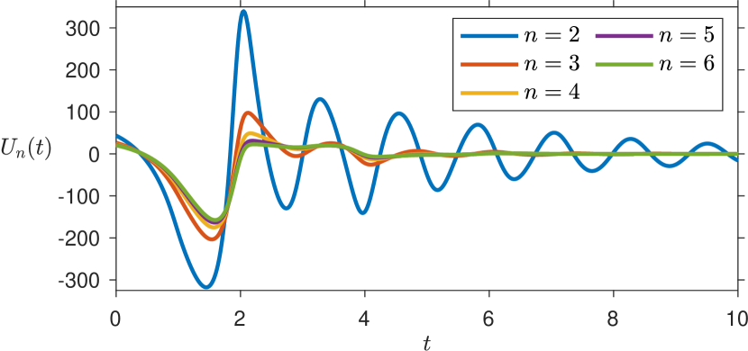
Figure 2: The controls $U(t)$ based on the approximate control law (16) when $n=2,\ldots,6$.

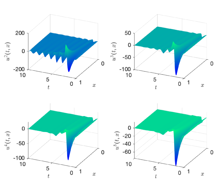
Figure 3: The solution component $u^{n}(t,x)$ when $n=2,\ldots,5$.

Fig. 2 and Fig. 3 show that the approximate control law based on the continuum kernels (54) is indeed stabilizing already when $n=2$, even if the rate of decay is very slow. However, Fig. 2 and Fig. 3 show that the closed-loop performance significantly improves when $n$ becomes larger, and in Fig. 2 the controls for $n=5$ and $n=6$ are virtually indistinguishable. However, as we consider larger values of $n$ separately in Fig. 4 and Fig. 5, some changes in $U(t)$ and $u^{n}(t,\xi)$ are still noticeable between $n=6$ and $n=10$. Regardless, in all studied cases beyond $n>5$, the controls, along with the solutions, have practically converged to zero by $t=6$. We note that it takes the control input $1/\mu+1/\lambda=2$ time units to traverse through the system (3), (4) for any $n$, which is why, e.g., the state component $u^{n}(t,\xi)$, may grow rapidly in the beginning of the simulation, as seen in Fig. 3 and Fig. 5, before getting stabilized by the controls. However, due to the in-domain coupling between $u$ and $v$ in (3), the controls do affect the $u^{i}$ components through $v$ already before entering the $u^{i}$ channels at time $t=1/\mu=1$.

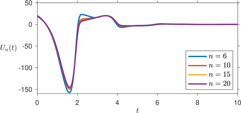
Figure 4: The controls $U(t)$ based on the approximate control law (16) when $n=6,10,15,20$.

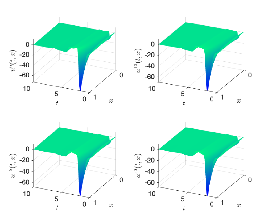
Figure 5: The solution component $u^{n}(t,x)$ when $n=6,10,15,20$.

Overall, the simulations demonstrate that the approximate control law (16) based on the continuum kernels (54) exponentially stabilizes the $n+1$ system (3), (4) when $n$ is sufficiently large, and that the approximation error of the control law decreases as $n$ increases. Thus, the simulations are well in accordance with the theoretical results. Moreover, in this example, the approximate control law has good performance already for very moderate $n$, showing that the sufficiently large $n$ appearing in the theoretical results may be, in practice, relatively small. However, one should not expect this to be the case in general, as this is dependent on the parameters of both the system (3), (4) and its continuum approximation (8), (9).

5.2 Comparison with Exact Control Kernels

In this subsection, we compare the approximate control gain kernels with the exact kernels, as well as we compare performance of the closed-loop systems under the approximate and exact kernels. However, as we are not aware of the existence of closed-form solutions to (6), (7), we have to find the solution implicitly, and hence, the presented comparisons are between the closed-form continuum kernels (54) and numerical approximations of the exact kernels obtained from (6), (7). Regardless, we refer to the numerical solution to (6), (7) as the exact kernels.

In Fig. 6, the evolution of $\displaystyle\max_{\xi\in[0,1]}\|\Delta\mathbf{k}(1,\xi)\|_{\infty}$ is shown for $n=2,3,\ldots,40$, where we use the boldface notation for the vector $\left(\Delta k^{i}\right)_{i=1}^{n+1}$. It can be seen that the error norm decays (even exponentially) as $n$ increases, until $n=17$ after which the accuracy of our numerical procedure to solving the exact kernel equations (6), (7) starts to deteriorate. That is, the increase in the error norm around $n=20$ is due to numerical inaccuracies in solving the exact kernel equations (6), (7), as in theory the error norm should tend towards zero as $n$ increases. Fig. 6 additionally shows the computational time required (by our numerical procedure) to solve (6), (7), which appears to grow linearly with respect to $n$. However, solving (6), (7) additionally requires spatial discretization of the domain $\mathcal{T}$, where we simply use finite differences with 257 grid points in both $x$ and $\xi$. We expect that (6), (7) can be solved more accurately using more sophisticated methods, such as finite element methods (FEM), and a finer discretization of $\mathcal{T}$, but this will likely result in longer computational times as well, since the complexity of FEM algorithms is proportional to the number of nodes in the finite element mesh [34]. We note here that the computational time of computing the approximate kernels is virtually invariant to $n$, as such computations rely only on evaluation of (54a) at the given points in $y$.

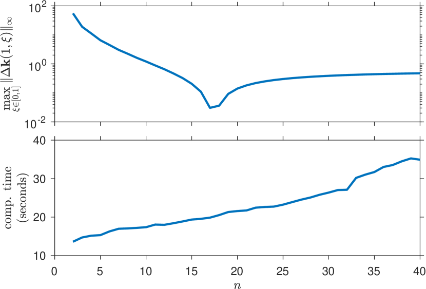
Figure 6: Top: Approximation error of the exact control kernels by the continuum control kernels. Bottom: Computational time to solving the exact control kernels PDEs.

In Fig. 7, we compare the control efforts obtained by using the approximate continuum kernels and the exact kernels obtained from (6), (7) for $n=3,5,10,20$. It can be seen that qualitatively the controls computed based on the exact kernels seem to behave the same despite of $n$. Moreover, as expected from Fig. 2 and Fig. 4, the approximate control laws computed based on the continuum kernels (54) get closer to the exact controls as $n$ increases. However, as already seen in Fig. 6, we can numerically demonstrate this convergence only up to some finite accuracy. Regardless, it can be seen from Fig. 7 that the differences in closed-loop performance are small already at $n=10$.

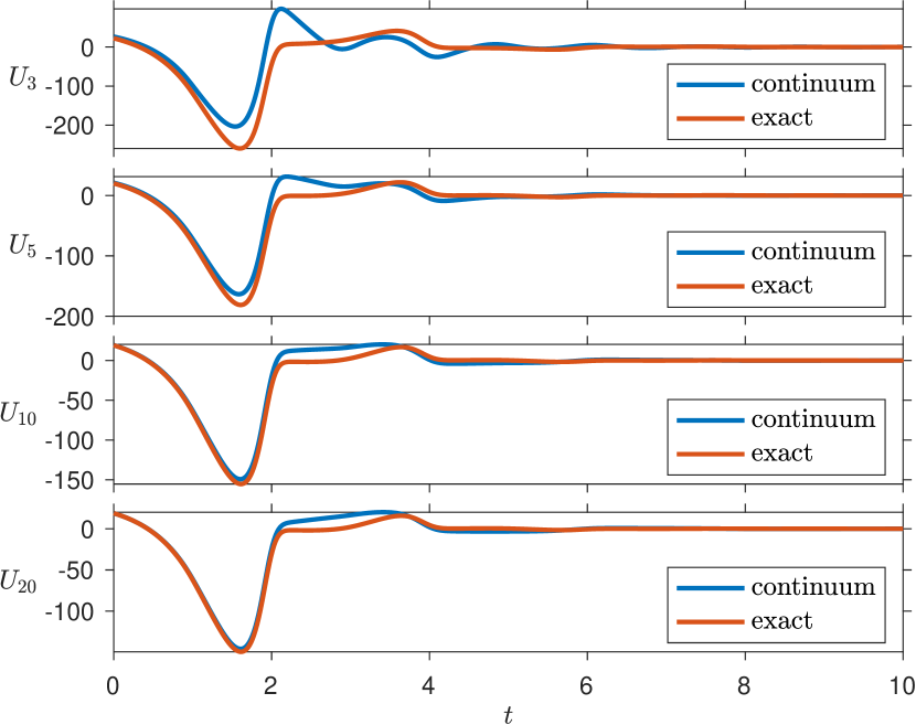
Figure 7: Comparison of the control efforts with the continuum (approximate) kernels and the exact control kernels for $n=3,5,10,20$.

6 Approximation of the Solutions to the Large-Scale System by a Continuum

In this section, we show that the continuum system (8), (9) acts as an approximation of the $n+1$ system (3), (4), when $n$ is sufficiently large. In particular, a sequence of solutions to (3), (4) can approximate the solution to (8), (9), provided that the sequence of data of (3), (4) approximates the data of (8), (9) (including initial conditions) to arbitrary accuracy.

Theorem 6.1.

Consider an $n+1$ system (3), (4), with parameters $\lambda_{i},\mu,W_{i},\theta_{i},\sigma_{i,j},q_{i}$ for $i,j=1,2,\ldots,n$ satisfying Assumption 2.1, initial conditions $v_{0},u_{0}^{i}\in L^{2}([0,1];\mathbb{R})$ for $i=1,2,\ldots,n$, and input $U\in L^{2}_{\rm{loc}}([0,+\infty);\mathbb{R})$. Construct a continuum system (8), (9), with parameters $\lambda,\mu,W,\theta,\sigma,q$ that satisfy Assumption 3.1 and (13), and equip (8), (9) with initial conditions $u_{0},v_{0}$ and input $U$, such that $u_{0}$ is continuous in $y$ and satisfies

$$u_{0}(x,i/n)=u_{0}^{i}(x),$$ (55)

for $i=1,2,\ldots,n$. Sample the solution $(u,v)$ to the resulting PDE system (8), (9) for these data, into a vector-valued function $\left((\widetilde{u_{i}})_{i=1}^{n},\widetilde{v}\right)$ as $\widetilde{\mathbf{u}}(t,x)=\mathcal{F}_{n}^{*}u(t,x,\cdot)$ and $\widetilde{v}(t,x)=v(t,x)$, pointwise for all $t\geq 0$ and almost all $x\in[0,1]$. On any compact interval $t\in[0,T]$, for any given $T>0$, we have

$$\max_{t\in[0,T]}\left\|\left(\begin{smallmatrix}\mathbf{u}(t)\\ v(t)\end{smallmatrix}\right)-\left(\begin{smallmatrix}\widetilde{\mathbf{u}}(t)\\ \widetilde{v}(t)\end{smallmatrix}\right)\right\|_{E}\leq\delta_{2}+\varepsilon_{2}+\delta_{3}+\varepsilon_{3},$$ (56)

where $\varepsilon_{2},\varepsilon_{3},\delta_{2},\delta_{3}>0$ become arbitrarily small when $n$ is sufficiently large.

Proof 6.2.

Firstly, we note that (8), (9) is well-posed on $E_{c}=L^{2}([0,1];L^{2}([0,1];\mathbb{R}))\times L^{2}([0,1];\mathbb{R})$ under Assumption 3.1 as shown in Proposition .2.1 in Appendix .2. That is, for any initial conditions $u_{0}\in L^{2}([0,1];L^{2}([0,1];\mathbb{R})),v_{0}\in L^{2}([0,1];\mathbb{R})$ and input $U\in L_{\rm{loc}}^{2}([0,+\infty);\mathbb{R})$, the solution $(u,v)$ is well-defined, unique, continuous in time, and depends continuously on the data of the problem on any compact interval $t\in[0,T]$, for any given $T>0$. In particular, there exist families of bounded linear operators $\mathbb{T}_{t},\Phi_{t}$ for $t\geq 0$, depending continuously on the parameters $\lambda,\mu,\sigma,\theta,W,q$, such that the solution to (8), (9) is given by [31, Prop. 4.2.5]

$$\left(\begin{smallmatrix}u(t)\\ v(t)\end{smallmatrix}\right)=\mathbb{T}_{t}\left(\begin{smallmatrix}u_{0}\\ v_{0}\end{smallmatrix}\right)+\Phi_{t}U,$$ (57)

which satisfies $\left(\begin{smallmatrix}u\\ v\end{smallmatrix}\right)\in C([0,+\infty);E_{c})$. The well-posedness and regularity of solutions to (3), (4) have already been established in Proposition .1.1 in Appendix .1 and Remark 2.2.

Secondly, based on the parameters $\lambda_{i},W_{i},\theta_{i},\sigma_{i,j},q_{i}$ for $i,j=1,2,\ldots,n$ of (3), (4), we can construct the step functions $\lambda^{n},\sigma^{n},\theta^{n},W^{n},q^{n}$ as in (17) such that they satisfy (29) for any $\varepsilon_{1}>0$ when $n$ is sufficiently large. Moreover, we can transform the solution to (3), (4) into a step function (in $y$) by applying the transform $\mathcal{F}$ introduced in the proof of Lemma 4.2, i.e.,

$$\left(\begin{smallmatrix}u^{n}(t,x,\cdot)\\ v^{n}(t,x)\end{smallmatrix}\right)=\mathcal{F}\left(\begin{smallmatrix}\mathbf{u}(t,x)\\ v(t,x)\end{smallmatrix}\right).$$ (58)

That is, $u^{n}$ is defined piecewise in $y$, for $i=1,2,\ldots,n$, as $u^{n}(t,x,y)=u^{i}(t,x)$, $y\in((i-1)/n,i/n]$, pointwise for all $t\in[0,T]$ and almost all $x\in[0,1]$. Then $(u^{n},v^{n})$ is the solution to (8), (9) for parameters $\lambda^{n},\mu,\sigma^{n},\theta^{n},W^{n},q^{n}$, input $U$, and initial conditions $v_{0},u_{0}^{n}(x,\cdot)=\mathcal{F}_{n}\mathbf{u}_{0}(x)$. This can be verified by applying the transform $\mathcal{F}$ to (3), (4) (from the left), for each $t\geq 0$ and almost all $x\in[0,1]$, which results in $(u^{n},v^{n})$ satisfying (8), (9) for the stated parameters, initial conditions, and input. (This follows in a similar manner with the respective part of the proof of Lemma 4.2.) As (3), (4) is well-posed, the transformed solution (3), (4) is the well-posed solution to the transformed (by $\mathcal{F}$) PDE system. In particular, there exist families of operators $\mathbb{T}_{t}^{n},\Phi_{t}^{n}$ for $t\geq 0$, depending continuously on the parameters $\lambda^{n},\mu,\sigma^{n},\theta^{n},W^{n},q^{n}$, such that the solution to (8), (9) for these parameters is given by

$$\left(\begin{smallmatrix}u^{n}(t)\\ v^{n}(t)\end{smallmatrix}\right)=\mathbb{T}^{n}_{t}\left(\begin{smallmatrix}u_{0}^{n}\\ v_{0}\end{smallmatrix}\right)+\Phi^{n}_{t}U,$$ (59)

which satisfies $\left(\begin{smallmatrix}u^{n}\\ v^{n}\end{smallmatrix}\right)\in C([0,+\infty);E_{c})$.

Thirdly, consider the difference of the solutions (to (8), (9)) (57) and (59), under the respective parameters and initial conditions, and the same inputs on the interval $t\in[0,T]$. We get, for each $t\in[0,T]$,

$$\left\|\left(\begin{smallmatrix}u(t)\\ v(t)\end{smallmatrix}\right)-\left(\begin{smallmatrix}u^{n}(t)\\ v^{n}(t)\end{smallmatrix}\right)\right\|_{E_{c}} \leq\left\|\left(\mathbb{T}_{t}-\mathbb{T}_{t}^{n}\right)\left(\begin{smallmatrix}u_{0}^{n}\\ v_{0}\end{smallmatrix}\right)\right\|_{E_{c}}$$

$$\quad+\left\|\mathbb{T}_{t}\right\|_{\mathcal{L}(E_{c})}\left\|\left(\begin{smallmatrix}u_{0}\\ v_{0}\end{smallmatrix}\right)-\left(\begin{smallmatrix}u_{0}^{n}\\ v_{0}\end{smallmatrix}\right)\right\|_{E_{c}}$$

$$\quad+\left\|\left(\Phi_{t}-\Phi_{t}^{n}\right)U\right\|_{E_{c}}$$

$$\leq\delta_{2}+\varepsilon_{2}+\delta_{3},$$ (60)

where, for any given $T,u_{0},v_{0}$, and $U$, the constants $\delta_{2},\varepsilon_{2},\delta_{3}$ can be made arbitrarily small by taking $n$ sufficiently large. That is, $\delta_{2}$ and $\delta_{3}$ become small due to the solution to (8), (9) depending continuously on the parameters, initial conditions, and input of the problem, i.e., $\delta_{2}$ and $\delta_{3}$ depend continuously on $\varepsilon_{1}$ in (29) such that $\delta_{2},\delta_{3}\to 0$ as $\varepsilon_{1}\to 0$. The second term $\varepsilon_{2}$ becomes small as $\left\|\mathbb{T}_{t}\right\|_{\mathcal{L}(E_{c})}$ is uniformly bounded on $t\in[0,T]$ by Proposition .2.1; while the difference $\|u_{0}-u_{0}^{n}\|_{L^{2}([0,1]^{2};\mathbb{R})}$ can be made arbitrarily small due to (55) and $u_{0}^{n}(x,\cdot)=\mathcal{F}_{n}\mathbf{u}_{0}(x)$, analogously to (29).

Finally, set $\widetilde{\mathbf{u}}(t,x)=\mathcal{F}_{n}^{*}u(t,x,\cdot)$ and $\widetilde{v}=v$ for all $t\in[0,T]$ and almost all $x\in[0,1]$, i.e., each component of $\widetilde{\mathbf{u}}$ is

$$\widetilde{u}^{i}(t,x)=n\int\limits_{(i-1)/n}^{i/n}u(t,x,y)dy,$$ (61)

which is the mean value of $u(t,x,\cdot)$ over an interval of length $1/n$ in $y$. Since $\mathcal{F}$ is an isometry, we have, for each $t\in[0,T]$,

$$\left\|\left(\begin{smallmatrix}\mathbf{u}(t)\\ v(t)\end{smallmatrix}\right)-\left(\begin{smallmatrix}\widetilde{\mathbf{u}}(t)\\  \widetilde{v}(t)\end{smallmatrix}\right)\right\|_{E} =\left\|\mathcal{F}\left(\left(\begin{smallmatrix}\mathbf{u}(t)\\ v(t)\end{smallmatrix}\right)-\left(\begin{smallmatrix}\widetilde{\mathbf{u}}(t)\\  \widetilde{v}(t)\end{smallmatrix}\right)\right)\right\|_{E_{c}}$$

$$\leq\left\|\left(\begin{smallmatrix}u^{n}(t)\\ v^{n}(t)\end{smallmatrix}\right)-\left(\begin{smallmatrix}u(t)\\ v(t)\end{smallmatrix}\right)\right\|_{E_{c}}$$

$$\quad+\left\|\left(\begin{smallmatrix}u(t)\\ v(t)\end{smallmatrix}\right)-\mathcal{F}\mathcal{F}^{*}\left(\begin{smallmatrix}u(t)\\ v(t)\end{smallmatrix}\right)\right\|_{E_{c}}$$

$$\leq\delta_{2}+\varepsilon_{2}+\delta_{3}+\varepsilon_{3},$$ (62)

where we used the triangle inequality (added and subtracted $(u,v)$), definitions (58) and (61), and (6.2). Moreover, $\varepsilon_{3}>0$ can be made arbitrarily small, as the solution $(u,v)$ is uniformly bounded on $t\in[0,T]$ and the step function $\mathcal{F}\mathcal{F}^{*}\left(\begin{smallmatrix}u(t)\\ v(t)\end{smallmatrix}\right)$ can approximate $\left(\begin{smallmatrix}u(t)\\ v(t)\end{smallmatrix}\right)$ to arbitrary accuracy (for almost all $x,y\in[0,1]$, uniformly in $t\in[0,T]$) when $n$ is sufficiently large, i.e., when the interval length $1/n$ becomes sufficiently small (by mean-value approximation, see, e.g., [32, Sect. 1.6]). Thus, the maximum of (6.2) over $t\in[0,T]$ can be made arbitrarily small by taking $n$ sufficiently large, which yields (56).

Remark 6.3.

The conclusion of Theorem 6.1 remains valid even if the input $U$ was not exactly the same for both PDE systems. That is, rewriting (6.2) with $U$ replaced by some $\bar{U}$ in (57) results in an additional error term $\|\Phi_{t}\|_{\mathcal{L}(L^{2}([0,T];\mathbb{R});E_{c})}\|U-\bar{U}\|_{L^{2}([0,T],\mathbb{R})}$, which can be made arbitrarily small by assuming $\|U-\bar{U}\|_{L^{2}([0,T],\mathbb{R})}$ is sufficiently small, since the operator norm of $\Phi_{t}$ is uniformly bounded on compact intervals $t\in[0,T]$ (based on Proposition .2.1 in Appendix .2).

7 The Limiting Case $n\to\infty$

While the system (3), (4) and the kernel equations (6), (7) are well-defined for any finite $n$, we can consider the limiting case $n\to\infty$ through interpreting these as the respective continuum limits of system (8), (9) and kernel equations (11), (12). This can be formally proved as follows, utilizing the results of Sections 4 and 6. As regards the case of the kernels, it follows from (28) that

$$\lim_{n\to\infty}\max_{(x,\xi)\in\mathcal{T}}\|k(x,\xi,\cdot)-k^{n}(x,\xi,\cdot)\|_{L^{2}([0,1];\mathbb{R})} =0,$$ (63a)

$$\lim_{n\to\infty}\max_{(x,\xi)\in\mathcal{T}}|\bar{k}(x,\xi)-\bar{k}^{n}(x,\xi)| =0.$$ (63b)

As proved in Lemma 4.4 (relation (29)), this convergence is enabled by the convergence of the respective parameters $\lambda^{n},\sigma^{n},\theta^{n},W^{n},q^{n}$ (constructed in (17), based on the parameters associated with the solution to (6), (7)) associated with the kernels constructed in (18) based on the solutions to (6), (7), to the parameters $\lambda,\sigma,\theta,W,q$ associated with the kernels satisfying (11), (12). Moreover, by (6.2), the solution sequence $(u^{n}(t),v^{n}(t))$, constructed in (58) based on the solutions to (3), (4), under the conditions of Theorem 6.1, converges (in $E_{c}$, on compact time intervals) to the solution of (8), (9), i.e.,

$$\lim_{n\to\infty}\left\|\left(\begin{smallmatrix}u(t)\\ v(t)\end{smallmatrix}\right)-\left(\begin{smallmatrix}u^{n}(t)\\ v^{n}(t)\end{smallmatrix}\right)\right\|_{E_{c}}=0,$$ (64)

for all $t\in[0,T]$, for any given $T>0$. Note that all convergence properties stated hold in $L^{2}$ for $y$, which is sufficient for attaining the stated approximation result. In fact, based on the convergence properties of the kernels and solutions, namely, equations (63) and (64), respectively, the control law (5) converges to (10) (on compact time intervals), i.e., the following holds

$$\lim_{n\to\infty}\int\limits_{0}^{1}\left[\frac{1}{n}\sum_{i=1}^{n}k^{i}(1,\xi)u^{i}(t,\xi)+k^{n+1}(1,\xi)v(t,\xi)\right]d\xi =$$

$$\lim_{n\to\infty}\left\langle\left(\begin{smallmatrix}\mathbf{k}(1,\cdot)\\ k^{n+1}(1,\cdot)\end{smallmatrix}\right),\left(\begin{smallmatrix}\mathbf{u(t)}\\ v(t)\end{smallmatrix}\right)\right\rangle_{E} =$$

$$\lim_{n\to\infty}\left\langle\left(\begin{smallmatrix}k^{n}(1,\cdot,\cdot)\\ \bar{k}^{n}(1,\cdot)\end{smallmatrix}\right),\left(\begin{smallmatrix}u^{n}(t)\\ v^{n}(t)\end{smallmatrix}\right)\right\rangle_{E_{c}} =$$

$$\left\langle\left(\begin{smallmatrix}k(1,\cdot,\cdot)\\ \bar{k}(1,\cdot)\end{smallmatrix}\right),\left(\begin{smallmatrix}u(t)\\ v(t)\end{smallmatrix}\right)\right\rangle_{E_{c}} =$$

$$\int\limits_{0}^{1}\left[\int\limits_{0}^{1}k(1,\xi,y)u(t,\xi,y)dy+\bar{k}(1,\xi)v(t,\xi)\right]d\xi,$$ (65)

for all $t\in[0,T]$, for any given $T>0$.

Finally, it is interesting to note that the stability estimate (51), based on the previous discussion, in the limiting case $n\to\infty$ becomes, essentially, the stability estimate of the continuum system (8), (9) under the exact continuum control law (10), i.e., (see also [27, Thm 2])

$$\left\|\left(\begin{smallmatrix}u(t)\\ v(t)\end{smallmatrix}\right)\right\|^{2}_{E_{c}}\leq\widetilde{M}^{C}_{V}\left\|\left(\begin{smallmatrix}u(0)\\ v(0)\end{smallmatrix}\right)\right\|^{2}_{E_{c}}\exp\left(-\frac{\bar{c}_{V}}{M^{C}_{V}}t\right),$$ (66)

where the coefficients $\widetilde{M}_{V}^{C},M_{V}^{C},\bar{c}_{V}$ are obtained based on the continuum counterparts of the respective coefficients in the Lyapunov-based proof of Theorem 4.1. This can be shown as follows. First, the solution $\left((u^{i}(t))_{i=1}^{n},v(t)\right)$ to (3), (4) converges to the solution $(u(t),v(t))$ to (8), (9) (via the step function interpretation (58); see Theorem 6.1 for details) as per (64), which results in the $E_{c}$ norms of $(u(t),v(t))$ and $(u_{0},v_{0})$ appearing in (66) and corresponding to the $E$ norm in (51). Second, combining the convergence property of each of the parameter sequences to their respective continuum limits, which follows from (29), together with the uniform essential boundedness of the parameter sequences, which follows from the step function-based construction, we can uniformly bound the functions appearing on the left-hand side of (42), and hence, also bound their continuum limits. In particular, $M_{\sigma}$ and $M_{W}$ can be replaced by

$$M_{\sigma}^{C} =\max_{x\in[0,1]}\|\sigma(x,\cdot,\cdot)\|_{L^{\infty}([0,1]^{2};\mathbb{R})},$$ (68)

$$M_{W}^{C} =\max_{x\in[0,1]}\|W(x,\cdot)\|_{L^{\infty}([0,1];\mathbb{R})}.$$ (69)

Similarly, we can replace $M_{\lambda}$ by $\displaystyle M_{\lambda}^{C}=\max_{x\in[0,1]}\|1/\lambda(x,\cdot)\|_{L^{\infty}([0,1];\mathbb{R})}$. Moreover, based on the convergence property (63), together with the essential boundedness of $(k^{n},\bar{k}^{n})$ (by construction), we can replace $M_{k}$ by

Consequently, as the inverse kernels $(l^{i})_{i=1}^{n+1}$ depend continuously on $(k^{i})_{i=1}^{n+1}$, while the parameters $(c_{i,j})_{i,j=1}^{n},(\kappa_{i})_{i=1}^{n}$ depend continuously on $(k^{i})_{i=1}^{n+1}$ and $(W_{i})_{i=1}^{n}$, we can construct step function sequences $(l^{n},\bar{l}^{n}),c^{n},\kappa^{n}$ (associated with parameters $l^{i},c_{i,j},\kappa_{i}$, in a similar manner to constructions (17), (18)), based on the step function sequences $(k^{n},\bar{k}^{n})$ and $W^{n}$. These sequences converge to their respective continuum limits $(l,\bar{l}),c,\kappa$ (in the $L^{2}$ sense in $y$), and they can be bounded, similarly to $(k^{n},\bar{k}^{n})$ and $W^{n}$. Thus, we can replace $M_{\kappa}$ and $M_{c}$ in (42), and $M_{l}$ in (46), by

$$M_{\kappa}^{C}=\max_{(x,\xi)\in\mathcal{T}}\|\kappa(x,\xi,\cdot)\|_{L^{\infty}([0,1];\mathbb{R})},$$ (71)

$$M_{c}^{C}=\max_{(x,\xi)\in\mathcal{T}}\|c(x,\xi,\cdot)\|_{L^{\infty}([0,1];\mathbb{R})},$$ (72)

(73)

Therefore, as $\delta,\epsilon\to 0$ in the limiting case $n\to\infty$, all involved parameters in estimate (51), namely $\widetilde{M}_{V},c_{V}$, and $M_{V}$, can be replaced by the continuum bounds $\widetilde{M}_{V}^{C},\bar{c}_{V}$ and $M_{V}^{C}$, based on (68)–(73), fact which allows us to obtain (66). We finally note that, by (64) and (7), the estimate (66) holds for all $t\in[0,T]$, for any given $T>0$, nevertheless, since (66) also provides a uniform bound for the solution, the estimate (66) is valid for all $t\in[0,+\infty)$.

8 Conclusions and Discussion

Computation of approximate stabilizing kernels based on the continuum kernel may provide flexibility in computation (also in terms of the number of different kernels being computed), as well as it may significantly improve computational complexity (although, practically, such computation also depends on the sampling method chosen for the continuum kernel). This is confirmed in the numerical example in which computational burden of stabilizing kernels is significantly improved, since the approximate kernels computed based on the continuum can be computed in closed form, in contrast to the exact kernels that have to be computed implicitly based on the solution to the kernel PDEs.

In general, we may expect that the complexity of computation of stabilizing control gains via the continuum approximation approach to not scale with $n$, i.e., to be $\mathcal{O}(1)$; while the complexity of computation of the exact control kernels to be $\mathcal{O}(n)$, i.e., to grow with the number of state components. Thus, this approach may be useful for computationally efficient control of large-scale PDE systems.

Another important possible usage of the approach presented may be in reducing the number of measurements required in a full-state feedback law, retaining closed-loop stability, in view of the fact that, as the number of state components increases, the sum in the control law (16) essentially approximates the integral in (10), which in turn may be computed at a chosen resolution, not necessarily equal to the number of state components. Although this is also motivated by simulation investigations we performed using the same numerical example as in Section 5, in which stability is preserved when we employ in (16) a smaller number, than $n$, of terms in the sum, this has to be rigorously proved. We have made here the first step towards such study by formally establishing the connection between the solutions to the original $n+1$ system (3), (4) and the solutions to the continuum system (8), (9), as the number $n$ of state components becomes sufficiently large. This is a matter we are currently investigating.

.1 Technical Propositions

This appendix contains two technical results regarding the well-posedness of the $n+1$ system (3), (4) under Assumption 2.1, and a generic result regarding exponential stability of perturbed, well-posed, infinite-dimensional linear systems. Both results are direct consequences of existing results in the literature.

Proposition .1.1.

The system (3), (4) is well-posed on $L^{2}([0,1];\mathbb{R}^{n+1})$ for any parameters satisfying Assumption 2.1.

Proof .1.2.

We utilize [30, Thm 13.2.2], for which we need to show that the system (3), (4) can be interpreted as a port-Hamiltonian system satisfying the assumptions of this theorem. Thus, we write the system (3) in the form $z_{t}(t,x)=P_{1}(\mathcal{H}(x)z(t,x))_{x}+D(x)z(t,x)$, where $z=(u^{1},\ldots,u^{n},v)^{T},P_{1}=\operatorname{diag}(-I_{n\times n},1)=P_{1}^{T},\mathcal{H}=\operatorname{diag}(\lambda_{1},\ldots,\lambda_{n},\mu)\in C^{1}([0,1];\mathbb{R}^{(n+1)\times(n+1)})$ by Assumption 2.1 and $D$ is a bounded linear operator. More precisely, $D=-P_{1}\mathcal{H}^{\prime}+D_{1}$, where $D_{1}$ is such that $D_{1}(x)z(x,t)$ corresponds to the right-hand-side of (3), and the the diagonal operator $P_{1}\mathcal{H}$ satisfies the first assumption of [30, Thm 13.2.2] by Assumption 2.1.

For the boundary conditions (4), we define a vector $f=(u^{1}(0),\ldots,u^{n}(0)$, $v(0),u^{1}(1),\ldots,u^{n}(1),v(1))^{T}$ comprising the boundary values of $z$. Using this, the boundary condition $u^{i}(\cdot,0)=q_{i}v(\cdot,0)$ can be written as $W_{B,1}f=0$, where $W_{B,1}=\begin{bmatrix}I_{n\times n}&-\mathbf{q}&0_{n\times(n+1)}\end{bmatrix}$, where we denote $\mathbf{q}=(q_{1},\ldots,q_{n})^{T}$. The boundary control $v(\cdot,1)=U(\cdot)$ can be written as $W_{B,2}f=U$, where $W_{B,2}=\begin{bmatrix}0&\ldots&0&1\end{bmatrix}$. Thus, the matrix $W_{B}=\begin{bmatrix}W_{B,1}\\ W_{B,2}\end{bmatrix}$ has full rank regardless of $\mathbf{q}$, which covers the second assumption of [30, Thm 13.2.2]. Thus, by [30, Thm 13.2.2, Rem. 13.2.3], the system (3), (4) is well-posed.

Proposition .1.3.

Consider a well-posed abstract Cauchy problem $\dot{z}(t)=Ax(t)+BU(t)$ on a Hilbert space $Z$ under feedback control law $U(t)=(K+\Delta K)z(t)$, where $K$ and $\Delta K$ are bounded linear operators. If the feedback law $U(t)=Kz(t)$ is exponentially stabilizing, then so is $U(t)=Kz(t)+\Delta Kz(t)$, provided that $\|\Delta K\|_{\mathcal{L}(Z,\mathbb{R})}$ is sufficiently small.

Proof .1.4.

The proof relies on the well-posedness of the abstract Cauchy problem, i.e., $B$ being an admissible control operator for (the strongly continuous semigroup generated by) $A$ [31, Sect. 4.2], and the Gearhart-Greiner-Prüss Theorem [35, Thm V.1.11]. Let us denote $A_{K}=A+BK$ which is the generator of an exponentially stable semigroup on $Z$, i.e., the solution to $\dot{z}(t)=(A+BK)z(t),z(0)=z_{0}$ satisfies $\|z(t)\|_{Z}\leq Me^{-\gamma t}\|z_{0}\|_{Z}$ for some $M,\gamma>0$. Now, the system under the perturbed control law can be written as $\dot{z}(t)=A_{K}z(t)+B\Delta Kz(t)$, where $B$ is admissible for $A_{K}$ by [31, Cor. 5.5.1]. Moreover, there exists some $K_{\gamma/4}>0$ such that [31, Prop. 4.4.6]

$$\|(sI-A_{K})^{-1}B\Delta K\|_{\mathcal{L}(Z)}$$

$$\qquad\leq\frac{K_{\gamma/4}}{\sqrt{\rm{Re}(s)+\gamma/4}}\|\Delta K\|_{\mathcal{L}(Z,\mathbb{R})},\quad\forall\operatorname{Re}(s)>-\gamma/4$$

$$\qquad\leq\frac{2K_{\gamma/4}}{\sqrt{\gamma}}\|\Delta K\|_{\mathcal{L}(Z,\mathbb{R})},\quad\forall\operatorname{Re}(s)>0,$$ (.1.1)

where, in place of $-\gamma/4$ we could use any value on $(-\gamma,0)$.

The rest of the proof utilizes spectral arguments. Based on the identity $(sI-A_{K}-B\Delta K)=(sI-A_{K})(I+(sI-A_{K})^{-1}B\Delta K)$, we see that any point $s\in\mathbb{C}$ is guaranteed to be in the resolvent set of $A_{K}+B\Delta K$ if it is in the resolvent set of $A_{K}$  and $\|(sI-A_{K})^{-1}B\Delta K\|_{\mathcal{L}(Z)}<1$. By the exponential stability of $A_{K}$ and (.1.4), these conditions can be guaranteed for all $\rm{Re}(s)>0$ when $\|\Delta K\|_{\mathcal{L}(Z,\mathbb{R})}$ is sufficiently small, in addition to the resolvent operator $(sI-A_{K}-B\Delta K)^{-1}$ being uniformly bounded for all $\rm{Re}(s)>0$. Thus, for $\|\Delta K\|_{\mathcal{L}(Z,\mathbb{R})}$  sufficiently small, we have that $A_{K}+B\Delta K$ is exponentially stable by [35, Thm V.1.11], which concludes the proof.

.2 Well-Posedness of the Continuum System

The following proposition states the well-posedness result for (8), (9), analogously to what has been stated in Proposition .1.1 for (3), (4).

Proposition .2.1.

The continuum system (8), (9) is well-posed on $E_{c}=L^{2}([0,1];L^{2}([0,1];\mathbb{R}))\times L^{2}([0,1];\mathbb{R})$ for any parameters satisfying Assumption 3.1. That is, for any initial conditions $u_{0}\in L^{2}([0,1];L^{2}([0,1];\mathbb{R})),v_{0}\in L^{2}([0,1];\mathbb{R})$ and input $U\in L_{\rm{loc}}^{2}([0,+\infty);\mathbb{R})$, there is a unique (weak) solution to (8), (9) satisfying $(u,v)\in C([0,+\infty);E_{c})$.

Proof .2.2.

In order to show the well-posedness of the continuum system (8), (9), due to [30, Lem. 13.1.14], we only need to show the well-posedness of the pure transport part, i.e.,

$$u_{t}(t,x,y)+\lambda(x,y)u_{x}(t,x,y) =0,$$ (.2.1a)

$$v_{t}(t,x)-\mu(x)v_{x}(t,x) =0,$$ (.2.1b)

with boundary conditions $u(t,0,y)=q(y)v(t,0),v(t,1)=U(t)$ and initial conditions $u(0,x,y)=u_{0}(x,y),v(0,x)=v_{0}(x)$. For now, assuming that everything is sufficiently smooth, the solution of the transport equation (.2.1) with spatially-varying transport speed is (cf. [36, Prop. 3.1])

$$v(t,x) =\begin{cases}v_{0}\left(\phi_{\mu}^{-1}(\phi_{\mu}(x)+t)\right),&t-\int\limits_{x}^{1}\frac{d\xi}{\mu(\xi)}\leq 0\\ U\left(t-\int\limits_{x}^{1}\frac{d\xi}{\mu(\xi)}\right),&t-\int\limits_{x}^{1}\frac{d\xi}{\mu(\xi)}>0\end{cases},$$ (.2.2a)

$$u(t,x,y) =\begin{cases}u_{0}\left(\phi_{\lambda_{y}}^{-1}(\phi_{\lambda_{y}}(x)-t),y\right),&t-\int\limits_{0}^{x}\frac{d\xi}{\lambda(\xi,y)}\leq 0\\ q(y)v\left(t-\int\limits_{0}^{x}\frac{d\xi}{\lambda(\xi,y)},0\right),&t-\int\limits_{0}^{x}\frac{d\xi}{\lambda(\xi,y)}>0\end{cases},$$ (.2.2b)

where $\phi_{\mu}(x)=\int_{0}^{x}\frac{d\xi}{\mu(\xi)}$ and $\phi_{\lambda_{y}}(x)=\int_{0}^{x}\frac{d\xi}{\lambda(\xi,y)}$, pointwise for (almost) every $y\in[0,1]$. The solution (.2.2) is well-defined, unique, and depends continuously on $\lambda,\mu,v_{0},u_{0}$ and $U$. The solution formula (and thus, the properties of the solution) is valid for any $v_{0}\in H^{1}([0,1];\mathbb{R}),u_{0}\in H^{1}([0,1];L^{2}([0,1];\mathbb{R})),$ and $U\in H^{1}_{\rm{loc}}([0,+\infty);\mathbb{R})$ under the compatibility conditions $v_{0}(1)=U(0)$ and $u_{0}(0,y)=q(y)v_{0}(0)$, i.e., (.2.2) is the classical solution of (.2.1). Moreover, for any $v_{0}\in L^{2}([0,1];\mathbb{R}),u_{0}\in L^{2}([0,1];L^{2}([0,1];\mathbb{R}))$ and $U\in L^{2}_{\rm{loc}}([0,+\infty);\mathbb{R})$, we can construct a unique weak solution as the limit of a sequence of classical solutions [7, Sect. 2.1.3] due to $H^{1}$ being dense in $L^{2}$ (on one-dimensional intervals) by the Sobolev Embedding Theorem. Thus, the system (.2.1) is well-posed on $L^{2}([0,1];L^{2}([0,1];\mathbb{R}))\times L^{2}([0,1];\mathbb{R})$. Finally, since (8), (9) only differs from (.2.1) by a bounded additive perturbation (i.e., everything on the right-hand side of (8)), we have that (8), (9) is well-posed by [30, Lem. 13.1.14].

References

References

• [1] V. Bikia, “Non-invasive monitoring of key hemodynamical and cardiac parameters using physics-based modelling and artificial intelligence,” Ph.D. dissertation, EPFL, 2021.
• [2] P. Reymond, F. Merenda, F. Perren, D. Rufenacht, and N. Stergiopulos, “Validation of a one-dimensional model of the systemic arterial tree,” Am. J. Physiol. Heart Circ. Physiol., vol. 297, pp. H208–H222, 2009.
• [3] L. Guan, C. Prieur, L. Zhang, C. Prieur, D. Georges, and P. Bellemain, “Transport effect of COVID-19 pandemic in France,” Annu. Rev. Control, vol. 50, pp. 394–408, 2020.
• [4] J. Friedrich, S. Göttlich, and M. Osztfalk, “Network models for nonlocal traffic flow,” ESAIM Math. Model. Numer. Anal., vol. 56, no. 1, pp. 213–235, 2022.
• [5] L. Zhang, H. Luan, Y. Lu, and C. Prieur, “Boundary feedback stabilization of freeway trafficnetworks: ISS control and experiments,” IEEE Trans. Control Syst. Technol., vol. 30, pp. 997–1008, 2022.
• [6] L. Tumash, C. Canudas-de-Wit, and M. L. Delle Monache, “Multi-directional continuous traffic model for large-scale urban networks,” Transportation Research Part B: Methodological, vol. 158, pp. 374–402, 2022.
• [7] G. Bastin and J.-M. Coron, Stability and Boundary Sabilization of 1-D Hyperbolic Systems, ser. Progress in Nonlinear Differential Equations and their Applications.   Birkhäuser/Springer, [Cham], 2016, vol. 88, subseries in Control.
• [8] J. Auriol and D. Bresch-Pietri, “Robust state-feedback stabilization of an underactuated network of interconnected $n+m$ hyperbolic PDE systems,” Automatica, vol. 136, p. 110040, 2022.
• [9] M. Krstic and A. Smyshlyaev, Boundary Control of PDEs: A Course on Backstepping Designs.   SIAM, 2008.
• [10] J. Auriol, “Output feedback stabilization of an underactuated cascade network of interconnected linear PDE systems using a backstepping approach,” Automatica, vol. 117, p. 108964, 2020.
• [11] L. Hu, F. Di Meglio, R. Vazquez, and M. Krstic, “Control of homodirectional and general heterodirectional linear coupled hyperbolic PDEs,” IEEE Trans. Automat. Control, vol. 61, no. 11, pp. 3301–3314, 2016.
• [12] J. Redaud, J. Auriol, and S.-I. Niculescu, “Output-feedback control of an underactuated network of interconnected hyperbolic PDE-ODE systems,” Systems Control Lett., vol. 154, p. 104984, 2021.
• [13] F. Di Meglio, R. Vazquez, and M. Krstic, “Stabilization of a system of $n+1$ coupled first-order hyperbolic linear PDEs with a single boundary input,” IEEE Trans. Automat. Control, vol. 58, no. 12, pp. 3097–3111, 2013.
• [14] T. Enderes, J. Gabriel, and J. Deutscher, “Cooperative output regulation for networks of hyperbolic systems using adaptive cooperative observers,” Automatica, vol. 162, p. 111506, 2024.
• [15] L. Paunonen and J.-P. Humaloja, “On robust regulation of PDEs: from abstract methods to PDE controllers,” in IEEE Conference on Decision and Control, 2022, pp. 7352–7357.
• [16] V. D. Blondel, J. M. Hendrickx, and J. N. Tsitsiklis, “On Krause’s multi-agent consensus model with state-dependent connectivity,” IEEE Trans. Automat. Control, vol. 54, no. 11, pp. 2586–2597, 2009.
• [17] G. Ferrari-Trecate, A. Buffa, and M. Gati, “Analysis of coordinations in multi-agent systems through partial difference equations,” IEEE Trans. Automat. Control, vol. 51, no. 6, pp. 1058–1063, 2006.
• [18] T. Meurer and M. Krstic, “Finite-time multi-agent deployment: A nonlinear PDE motion planning approach,” Automatica, vol. 37, pp. 2534–2542, 2011.
• [19] D. Nikitin, C. Canudas-de-Wit, and P. Frasca, “A continuation method for large-scale modeling and control: from ODEs to PDE, a round trip,” IEEE Trans. Automat. Control, vol. 67, pp. 5118–5133, 2022.
• [20] J. Wei, E. Fridman, and K. H. Johansson, “A PDE approach to deployment of mobile agents under leader relative position measurements,” Automatica, vol. 106, pp. 47–53, 2019.
• [21] J. Qi, R. Vazquez, and M. Krstic, “Multi-agent deployment in 3-D via PDE control,” IEEE Trans. Automat. Control, vol. 60, no. 4, pp. 891–906, 2015.
• [22] P. Frihauf and M. Krstic, “Leader-enabled deployment into planar curves: A PDE-based approach,” IEEE Trans. Automat. Control, vol. 56, pp. 1791–1806, 2011.
• [23] J. Zhang, R. Vazquez, J. Qi, and M. Krstic, “Multi-agent deployment in 3-D via reaction-diffusion system with radially-varying reaction,” Automatica, vol. 161, p. 111491, 2024.
• [24] L. Bhan, Y. Shi, and M. Krstic, “Neural operators for bypassing gain and control computations in PDE backstepping,” IEEE Trans. Automat. Control, 2024, early access.
• [25] J. Auriol, K. A. Morris, and F. Di Meglio, “Late-lumping backstepping control of partial differential equations,” Automatica, vol. 100, pp. 247–259, 2019.
• [26] R. Vazquez, G. Chen, J.-F. Qiao, and M. Krstic, “The power series method to compute backstepping kernel gains: Theory and practice,” in IEEE Conference on Decision and Control, 2023.
• [27] V. Alleaume and M. Krstic, “Ensembles of hyperbolic PDEs: stabilization by backstepping,” arXiv, 2307.13195, 2023.
• [28] I. Atamas, S. Dashkovskiy, and V. Slynko, “Lyapunov functions for linear hyperbolic systems,” IEEE Trans. Automat. Control, vol. 68, pp. 6496–6508, 2023.
• [29] A. Terrand-Jeanne, V. Andrieu, V. Dos Santos, and C.-Z. Xu, “Adding integral action for open-loop exponentially stable semigroups and application to boundary control of PDE systems,” IEEE Trans. Automat. Control, vol. 65, no. 11, pp. 4481–4492, 2020.
• [30] B. Jacob and H. Zwart, Linear Port-Hamiltonian Systems on Infinite-dimensional Spaces, ser. Operator Theory: Advances and Applications.   Birkhäuser, 2012, vol. 223.
• [31] M. Tucsnak and G. Weiss, Observation and Control for Operator Semigroups.   Birkhäuser Verlag AG, 2009.
• [32] T. Tao, An Introduction to Measure Theory.   American Mathematical Society, 2011.
• [33] R. Vazquez and M. Krstic, “Marcum Q-functions and explicit kernels for stabilization of $2\times 2$ linear hyperbolic systems with constant coefficients,” Syst. Control Lett., vol. 68, pp. 33–42, 2014.
• [34] I. Farmaga, P. Shmigelskyi, P. Spiewak, and L. Ciupinski, “Evaluation of computational complexity of finite element analysis,” in The Experience of Designing and Application of CAD Systems in Microelectronics (CADSM), 2011, pp. 213–214.
• [35] K.-J. Engel and R. Nagel, One-Parameter Semigroups for Linear Evolution Equations.   Springer, 2000.
• [36] J.-M. Coron, R. Vazquez, M. Krstic, and G. Bastin, “Local exponential $H^{2}$ stabilization of a $2\times 2$ quasilinear hyperbolic system using backstepping,” SIAM J. Control Optim., vol. 51, no. 3, pp. 2005–2035, 2013.