EDA-Driven Preprocessing for SAT Solving

Abstract

Effective formulation of problems into Conjunctive Normal Form (CNF) is critical in modern Boolean Satisfiability (SAT) solving for optimizing solver performance. Addressing the limitations of existing methods, our Electronic Design Automation (EDA)-driven preprocessing framework introduces a novel methodology for preparing SAT instances, leveraging both circuit and CNF formats for enhanced flexibility and efficiency. Central to our approach is the integration of a new logic synthesis technique, guided by a reinforcement learning agent, and a novel cost-customized LUT mapping strategy, enabling efficient handling of diverse SAT challenges. By transforming the SAT competition benchmarks into circuit instances, our framework demonstrates substantial performance improvements, as evidenced by a $52.42\%$ reduction on average compared to solving directly. Moreover, our framework achieves a remarkable $96.14\%$ runtime reduction on average for a set of logic equivalence checking problems that exhibit inherent circuit structures. These results highlight the effectiveness and versatility of our approach in handling both CNF and circuit instances. The code is available at https://github.com/cure-lab/EDA4SAT.

1 Introduction

In the realm of computational problem-solving, the Boolean Satisfiability (SAT) problem holds a pivotal position, which involves determining the truth of a Boolean formula under variable assignments. Identified as the first NP-complete problem [10], SAT’s complexity and versatility have captivated researchers for decades. SAT solvers [36, 16], central in addressing these problems, predominantly rely on Conjunctive Normal Form (CNF). CNF represents problems as an intersection of simpler clauses, a format that both challenges and drives innovation in SAT solving.

The dominance of CNF in SAT solving necessitates the conversion of diverse SAT problems into this format, be they graph-based, circuit-based, or pure Boolean formulas. Research spanning decades highlights the profound impact of CNF representation on problem-solving efficiency [41, 38]. A variety of preprocessing methods have emerged to refine CNF construction and transformation, optimizing the initial stages of the SAT solving process [12, 3, 39, 9]. Despite these developments, current SAT solving approaches continue to encounter significant challenges, underscoring the need for further innovation.

A major challenge within the existing SAT solving framework is the absence of a universally efficient formulation mechanism. In practical scenarios, SAT problems are often directly transformed into SAT instances, bypassing optimized constructions. This unrefined mapping often results in significantly larger problem sizes [3]. While various preprocessing techniques have been developed to compress the CNF formulae [30, 14, 37, 15], their effectiveness is not guaranteed. For instance, even seemingly small verification tasks can require hours to resolve [27], suggesting that simple CNF reduction may not suffice for efficient problem solving [9].

Moreover, several SAT preprocessing methods have been tailored for specific applications, such as microprocessor verification [39] and scheduling problems [12]. Although these methods perform well within their respective domains, their lack of adaptability to other problem types reveals a significant gap in the current approach to SAT preprocessing, highlighting the need for more universally applicable solutions.

To address these challenges, we introduce an Electronic Design Automation (EDA)-driven preprocessing framework, a novel integration into the standard SAT solving pipeline. This framework begins by converting CNF into a circuit format and then strategically reformulates the circuit representation. The process culminates in reverting the circuit back to an optimized CNF format, tailored for more efficient solving. This method’s flexibility in transitioning between circuit and CNF formats enables the application of advanced circuit transformation techniques across diverse SAT problems.

In our framework, we leverage EDA solutions to harness the detailed structural information of circuits for SAT problem reformulation. Central to this approach is the use of logic synthesis, augmented by a reinforcement learning (RL) agent dedicated to identifying optimal logic synthesis strategies. In contrast to traditional methods [15] focusing primarily on size reduction, our RL agent is specifically trained to minimize overall SAT solving complexity. The RL agent utilizes DeepGate [34], a sophisticated gate-level representation technique, for capturing rich information from initial problem instances. Additionally, we integrate a cost-customized look-up table (LUT) mapping strategy. Again, our approach maps the circuit into a format that is inherently easier to solve, diverging from conventional mappings aimed at compact design.

By integrating this EDA-driven preprocessing framework with the baseline SAT solver Kissat [16], we have achieved a remarkable average solving time reduction of $96.14\%$ for a set of circuit equivalence checking problems, compared to applying the baseline solver directly. Furthermore, we convert the CNF instances into circuits and then process circuits by our framework. Our framework demonstrates impressive versatility in effectively accelerating the solving process for a variety of problems in the SAT competition benchmarks with an average reduction in runtime of $52.42\%$.

We summarize the contributions of this work as follows:

• Introduction of an innovative EDA-driven preprocessing framework that seamlessly integrates into the SAT solving pipeline, efficiently reformulating SAT problems by converting standard CNF formulas into circuits and optimizing them for easier solving. Additionally, the proposed framework is not mutually exclusive with the existing CNF-based preprocessing strategy.

• Implementation of logic synthesis techniques guided by an RL agent, designed to explore optimal logic synthesis strategies and directly minimize the solving complexity.

• Integration of a cost-customized LUT mapping approach that not only conceals redundant logic during solving, but also significantly enhances the reduction of solving complexity.

2 Related Work

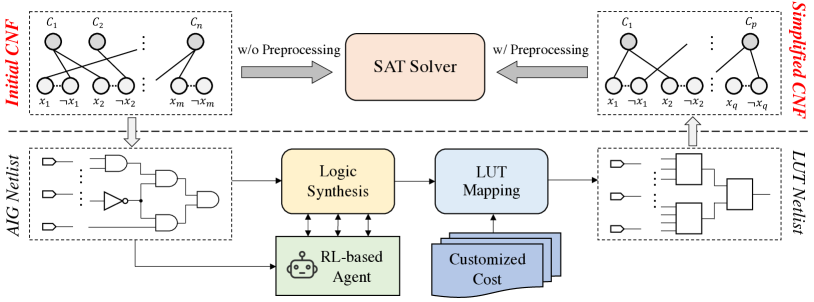
Figure 1: Overview of EDA-Driven SAT preprocessing framework

2.1 SAT Preprocessing

Conjunctive Normal Form (CNF) has become a standard format in modern SAT solvers, capable of representing arbitrary Boolean formulas. It is structured as a conjunction of clauses, denoted by $\phi=(C_{1}\land C_{2}\land\ldots)$, with each clause being a disjunction of variables or their negations, e.g., $C_{i}=(x_{1}\lor\neg x_{2}\lor\ldots)$. Over recent decades, numerous CNF-based heuristics have been developed to enhance SAT solving efficiency, including advanced clause management strategies [1] and innovative branching heuristics [29, 33].

While some studies [39, 12] have successfully modeled practical problems into CNFs, their specificity often limits generalizability to diverse problem sets. Commonly, real-world problems are converted directly into CNF, leading to redundant clauses and increased complexity. For example, a tournament scheduling problem with $n$ teams can escalate to $n^{6}$ clauses [3].

There are some works dedicated to CNF reformulation [14, 37], but the flattened structure and the lack of semantic information of CNF often require repetitively resolving clauses to establish logical relationships, which is time-intensive. Efforts like [30, 15] target recovering structures from CNF and minimizing the instances, but they cannot promise to reduce SAT solving time. In our work, we introduce a comprehensive preprocessing framework designed to directly reduce solving time.

2.2 Boolean Circuit Optimization

Boolean circuits, representable as directed acyclic graphs (DAGs) $\mathcal{G}(\mathcal{V},\mathcal{E})$ with logic gates and wires serving as nodes $\mathcal{V}$ and edges $\mathcal{E}$, respectively, are pivotal in computational logic. In EDA community, a wealth of efficient algorithms has been developed for circuit optimization. Logic synthesis is a prime example, involving DAG-based transformation techniques to modify circuit’s local structure for the optimization of performance, power, and area (PPA).

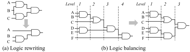
Figure 2: Example of logic rewrite and balance

We provide the examples of two logic synthesis methods that are supported by common EDA tools [7, 40]: rewrite and balance (see Figure 2). Logic rewrite (rewrite) is a circuit optimization technique that aims to minimize the overall circuit structure [6, 26]. The rewrite tools pre-compute and store all optimal circuits within $4$ inputs. When applied to an arbitrary circuit, the tools iteratively identify sub-graph and subsequently replace it with functionally-equivalent but smaller sub-graph. Balance (balance) [11] creates an equivalent circuit with the minimum possible delay, i.e., the minimum number of logic levels. As suggested by its name, this method achieves optimization by balancing the fan-in regions of multi-input gates within the circuit.

Besides, technology mapping, a key component in EDA flow, fine-tunes performance metrics under specific constraints [4] and maps the intermediate circuits into standard cells pre-defined in technology library. One widely used technique for technology mapping is Look-Up Table (LUT) mapping [17]. LUT mapping involves the transformation of gate combinations into $k$-LUTs, where each $k$-LUT represents a configurable memory unit capable of implementing arbitrary Boolean functions with $k$ variables.

In this work, we introduce a novel approach where logic synthesis techniques are employed to simplify the solving complexity of circuit instances, rather than conventional goal of optimizing area or delay. Our proposed framework integrates with open-source EDA tool ABC [7] to perform logic synthesis and utilize customized LUT mapping to generate simplified circuit instances composed of LUTs.

2.3 Circuit Representation Learning

Training a pre-trained model to learn general representations and subsequently fine-tuning it for specific tasks has become a prominent trend across various domains. Recently, there has been a growing focus on developing pre-trained models capable of deriving circuit general representations. DeepGate family [21, 34] is a series of circuit representation learning models. The first version DeepGate [21] proposes to introduce strong inductive bias into circuit data through logic synthesis and is supervised by the statistic random simulation results, which effectively reflect structural and functional features of circuits. DeepGate2 [34] further advances circuit representation learning by disentangling the structural and functional representations. Moreover, DeepGate2 showcases significantly faster inference runtimes compared to the predecessor while even learning better circuit representations. The gate-level representation vectors derived from the DeepGate model encapsulate the general circuit information, which proves instrumental in facilitating various EDA applications, such as testability analysis [32] and power estimation [20]. In this work, we tailor existing EDA tools for specific requirements, utilizing circuit knowledge learning capabilities of pre-trained DeepGate2 to inform our circuit optimization decisions.

3 Methodology

3.1 Overview of the Proposed Framework

Figure 1 shows the overview of proposed EDA-Driven SAT Preprocessing. Firstly, we convert the initial CNFs into And-Inverter Graph (AIGs) [5], which represent any logic behaviours only with three gate types: AND Gate, NOT Gate and Primary Input (PI). Then, we apply a predetermined sequence of AIG transformation operations to unify the distribution of input circuit [22].

Secondly, we utilize logic synthesis technique to reformulate SAT instance. Since the logic synthesis process can be considered as a sequential decision-making task, we train an agent to minimize the solving complexity by reinforcement learning (RL). In the RL framework, the state comprises embeddings of the initial AIG netlist and features of intermediate circuits. Additionally, the RL agent operates within a discrete action space, where each action corresponds to executing a synthesis operation. We approximate the complexity of SAT solving based on the number of variable branching times and define the reduction in branching times as the reward for RL agent.

Thirdly, we employ the LUT mapping technique to hide the internal logic of circuits. To further decrease the solving time, we design a cost-customized mapping operation with the objective of minimizing the branching times during SAT solving, rather than solely focusing on reducing the problem size. After the LUT mapping, we obtain the LUT netlist with a relatively small number of cells. To ensure compatibility with modern SAT solvers, we transform the LUT netlist back into a simplified CNF.

3.2 Logic Synthesis Recipe Exploration

We formulate logic synthesis as a Markov Decision Process (MDP) process, with the optimization objective of reducing the solving time for a given input instance. Consequently, such sequence decision-making process entails iteratively selecting a logic synthesis operation as an action according to the current circuit state.

3.2.1 Reinforcement Learning Formulation

To explore the optimal logic synthesis sequence (i.e. logic synthesis recipe), we employ Deep Q-learning algorithm in this section to train an reinforcement learning (RL) agent. The RL agent is trained to make informed decisions to minimize solving time by learning from its interactions with the circuit environment.

As shown in Figure 3, at each step $t$ (where $t=0,1,...,T-1$), the features of the current netlist $\mathcal{G}^{t}$ are extracted to form the state $s^{t}$. Subsequently, the Q-learning agent utilizes $s^{t}$ as input and selects an action $a^{t}$. Then, the environment including the logic synthesis tool performs the synthesis operation based on $a^{t}$ and transforms the netlist $\mathcal{G}^{t}$ into a new netlist $\mathcal{G}^{t+1}$. At the end of this step, the environment provides RL agent with a reward $r^{t}$. The above process is repeated for subsequent steps until $t=T-1$. During the training process, the objective of RL agent is to maximize the cumulative sum of the reward values. As a result, the trained RL agent is able to select logic synthesis operations step by step to achieve the optimal solving time reduction.

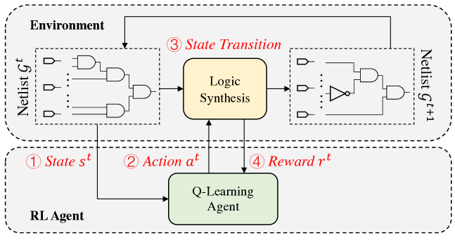
Figure 3: RL Agent-Environment interaction

3.2.2 State

Inspired by [19, 42], we extract the following representative features $\mathcal{E}(\mathcal{G}^{t})$ of the netlist $\mathcal{G}^{t}$ into state $s^{t}$:

• The ratio between the area of netlist $\mathcal{G}^{t}$ and netlist $\mathcal{G}^{0}$.

• The ratio between the depth of netlist $\mathcal{G}^{t}$ and netlist $\mathcal{G}^{0}$.

• The ratio between the wire counts of netlist $\mathcal{G}^{t}$ and netlist $\mathcal{G}^{0}$.

• The proportion of AND gates in the total gates of netlist $\mathcal{G}^{t}$.

• The proportion of NOT gates in the total gates of netlist $\mathcal{G}^{t}$.

• The average balance ratio of netlist $\mathcal{G}^{t}$. We formally define the average balance ratio $br$ in Eq. (1), where $\mathcal{P}_{i1}$, $\mathcal{P}_{i2}$ are predecessors of two fanin AND gate $i$, and $d$ denotes the depth.

$$br=\sum_{i\in AND}\frac{abs(d_{\mathcal{P}_{i1}}-d_{\mathcal{P}_{i2}})}{max(d_{\mathcal{P}_{i1}},d_{\mathcal{P}_{i2}})}\ /\ \#AND$$ (1)

The above features exhibit characteristics that can be effectively optimized by various logic synthesis operations. Consequently, the RL agent can intelligently select appropriate operations based on these features. For example, when a netlist shows a higher average balance ratio, indicating an imbalanced structure in DAG, the agent is more inclined to select the action of operation balance. Additionally, a large area ratio prompts the agent to opt for operations that aim to minimize the circuit area, such as rewrite.

Besides, the state $s^{t}$ is incorporated with the primary output embeddings of the initial netlist obtained by pretrained DeepGate2 [34] (denoted as $\mathcal{D}(\mathcal{G}^{0})$), which contains rich structural and functional information of the initial problem instance.

$$s^{t}=\text{Concatenate}(\mathcal{E}(\mathcal{G}^{t}),\mathcal{D}(\mathcal{G}^{0}))$$ (2)

3.2.3 Action

The action space $\mathcal{A}$ of agent is discrete and encompasses logic synthesis operations. In this paper, we set the available operations as follows: rewrite [26], refactor [8], balance [11], resub [7] and end (marking the end of the logic synthesis process). The selection of these operations does not imply that the proposed framework lacks support for additional synthesis operations beyond this set. Instead, these operations are chosen due to their widespread usage and commonality. If there is a need to include additional optional operations, it can be accomplished by expanding the action space within the framework.

3.2.4 State Transition

The state transition function is implemented by the logic synthesis tool. We call the tool with a specific logic synthesis operation determined by RL agent to transform current netlist $\mathcal{G}^{t}$ to another functional-equivalent but simplified netlist. More formally, we note the given netlist as $\mathcal{G}^{t}$ and RL action as $a^{t}$ at step $t$. The state transition function is denoted as: $\mathcal{G}^{t+1}=\mathcal{F}(\mathcal{G}^{t},a^{t})$, where $\mathcal{G}^{t+1}$ is the updated netlist by tool. The updated netlist, $\mathcal{G}^{t+1}$, is then considered as the input for the subsequent decision step at time $t+1$.

3.2.5 Reward

We consider the reduction of variable branching times during SAT solving as the reward. The reward function is shown as Eq. (3), where $\Delta\#Branching$ is the difference in branching times between the final instance and the initial instance during solving. We opt for the terminated reward, which has only one non-zero reward value at the terminated step, i.e. after performing the entire sequence of synthesis operations.

$$r^{t}=\left\{\begin{aligned} &0,t=0,\cdots,T-2,\\ &\textnormal{-}\Delta\#Branching,\ t=T-1\ or\ a^{t}=\textit{end}\end{aligned}\right.$$ (3)

Prior to solving the SAT instance in circuit format, we employ the LUT mapping technique to convert the AIG netlist into an LUT netlist. Subsequently, the transformed netlist is converted into Conjunctive Normal Form (CNF), which will be elaborated in the following section. Additionally, we choose not to minimize the solver runtime based on two primary reasons. Firstly, determining the solver runtime for hard SAT instances is significantly time-consuming. Secondly, the solver runtime is challenging to calculate accurately due to the fluctuating CPU status in the case of easy SAT instances. We utilize variable branching times to approximate solving time. This approach allows us to include easy cases with short solver runtime in the training dataset, thereby enhancing the efficiency of training the RL agent.

3.2.6 Policy

In the Q-learning framework [28], the policy for maximizing the total reward entails selecting the action with the highest expected value. We implement the action-value function $Q$ using multilayer perceptron (MLP) to estimate the sum of future rewards after taking a certain action under current state. The policy $\pi(s^{t})$ and action-value function $Q_{\theta}(s^{t},a)$ are shown in Eq. (4), where the $\theta$ parametrizes the function $Q$.

$$\begin{split}\pi(s^{t})&=\arg\max_{a,a\in\mathcal{A}}(Q(s^{t},a))\\ Q_{\theta}(s^{t},a)&=Index(MLP(s^{t}),a)\end{split}$$ (4)

We create the target function $Q_{\hat{\theta}}(s^{t},a)$ to stabilize the training process. The parameter $\hat{\theta}$ are copied from $\theta$ after $k$ steps. The parameter $\theta$ of action-value function $Q$ is updated iteratively by loss function in Eq. (5), where $\gamma$ is a hyperparameter and represents discount factor.

$$l=||Q_{\theta}(s^{t},a^{t})-r^{t}-\gamma\arg\max_{a\in\mathcal{A}}Q_{\hat{\theta}}(s^{t+1},a)||_{2}$$ (5)

3.3 Cost-Customized LUT Mapping

We present a cost-customized LUT mapping approach that not only hides the internal nodes during solving, but also forms an easy-to-solve CNF instance. Unlike conventional mapping tools that focus on constructing circuits with low area or delay, our approach aims to create circuits that are easier to solve. Specifically, we begin by defining a cost metric to quantify the branching complexity of SAT solving and compute the cost values for all $4$-input LUTs. Next, we modify the cost function in the existing mapping tool to enable minimizing the overall branching complexity. Lastly, we apply the cost-customized mapper to map AIG netlist to LUT netlist and convert the LUT netlist into CNF.

3.3.1 Branching Complexity of LUT

The SAT solving process involves iteratively making variable branching decisions, where the solver selects variable assignments as either true or false. We formulate the solving process within the circuit domain. Specifically, given the logic value of a certain gate, the SAT solver is required to make decisions by selecting assignments for its fanin gates. We consider two 2-fanin LUTs, denoted as $L_{1}$ (representing an AND gate) and $L_{2}$ (representing an XOR gate), and list the truth tables for these LUTs in Figure 4.

We observe that both $L_{1}$ and $L_{2}$ have two possible combinations when the fanout pin (C) is logic-0. However, when the fanout pin is logic-1, $L_{2}$ has two possible combinations while $L_{1}$ has only one unique branch. We define the branching complexity $C$ as the total number of possible fanin combinations. In this example, the LUT $L_{1}$ has $C_{L_{1}}=3$ and LUT $L_{2}$ has $C_{L_{2}}=4$. Therefore, $L_{2}$ is more hard to be solved than $L_{1}$.

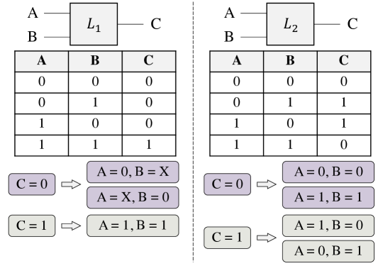
Figure 4: LUTs with different branching complexity

Input: The input CNF instance $\phi_{in}$ or Circuit instance $\mathcal{G}_{in}$

Output: The output simplified CNF instance $\phi_{out}$

/* Initialize circuit graph $\mathcal{G}^{0}$ in AIG */

1 if input instance is in CNF then

2       $\mathcal{G}^{0}=\textit{cnf2aig}(\phi_{in})$;

3      

4else

5       $\mathcal{G}^{0}=\textit{aigmap}(\mathcal{G}_{in})$;

6      

7 end if

8

/* Explore logic synthesis recipe by RL-agent (see Section 3.2) */

9 Define maximum step count: $T$;

10 t = 0;

11 while $t<T$ do

       /* Prepare the state of current circuit */

12       $s^{t}=\text{Concatenate}(\mathcal{E}(\mathcal{G}^{t}),\mathcal{D}(\mathcal{G}^{0}))$;

       /* Make decision to choose a logic synthesis operation */

13       $a^{t}=\pi(s^{t})=\arg\max_{a,a\in\mathcal{A}}(Q(s^{t},a))$;

14       if $a^{t}$ is end then

15             break;

16            

17       end if

      /* Perform logic synthesis for state transition */

18       $\mathcal{G}^{t+1}=\mathcal{F}(\mathcal{G}^{t},a^{t})$;

19       $t=t+1$;

20      

21 end while

22

/* Perform cost-customized LUT mapping (see Section 3.3) */

23 Define LUT costs: $C$ ;

24 $\mathcal{G}_{LUT}=\textit{mapper}(\mathcal{G}^{t},C)$;

/* Convert back to CNF */

25 $\phi_{out}=\textit{lut2cnf}(\mathcal{G}_{LUT})$;

26 return $\phi_{out}$;

Algorithm 1 EDA-Driven preprocessing framework for SAT solving

3.3.2 Cost-Customized Mapper

Since a large number of possible branches result in an exponential search space, various heuristics [23, 25] are employed to reduce the number of potential branches and improve the efficiency of the solving process. Besides, utilizing techinque mapping tools facilitates the concealment of intermediate gates and decreases the overall number of branches [15].

In contrast to [15] that minimizes the size of the post-mapping netlist, our approach prioritizes mapping the logic into cells with lower branching complexity. Our approach is motivated by the observations that instances containing a significant proportion of XOR gates often require more time to be solved [18, 13], where the the branching complexity of XOR gate ($L_{2}$ in Figure 4) is higher than other gates.

To prioritize the LUTs during mapping process, we employ a strategy whereby we enumerate all $4$-LUTs and integrate their branching complexity into the cost function. We implement a cost-customized mapper based on mockturtle [35] by modifying the area cost to reflect the branching complexity of each LUT and fixing the the delay cost as a constraint. By executing a sequence of operations aimed at minimizing the total cost, the resulting post-mapping netlists exhibit minimal overall branching complexity. To ensure the compatibility of CNF-based SAT solver, our preprocessing strategy ends with a LUT to CNF transformation [24].

As a result, we formally depict our overall EDA-driven preprocessing framework coupled with RL-based logic synthesis exploration and cost-customized LUT mapping in Algorithm 1. The framework begins by transforming the input CNF instance $\phi_{in}$ or circuit instance $\mathcal{G}_{in}$ into AIG format, using either $cnf2aig$ tool [31] or $aigmap$ technique in ABC [7]. Then, the RL agent (elaborated in Section 3.2) proceeds to select logic synthesis operations step by step through making action $a^{t}$. During this process (line 6-16), the circuit is synthesized multiple times to create a simplified circuit. Next, the framework continues to perform cost-customized LUT mapping on the AIG netlist $\mathcal{G}^{t}$, resulting in a compact LUT netlist $\mathcal{G}$. Finally, the LUT netlist is encoded into CNF as output $\phi_{out}$. Due to these simplification approaches, $\phi_{out}$ has a lower solving complexity than $\phi_{in}$ and the subsequent SAT solving procedures can be more efficiently. We will assess the effectiveness of our preprocessing by the following experiments.

4 Experiments

4.1 Experiment Settings

We collect $200$ industrial instances in AIG format into the RL training dataset. These AIG instances are derived from logic equivalence checking (LEC) problems and only contain a single primary output. The statistics of these instances are shown in Table 1, where # Clauses shows the number of clauses after transforming the AIG instances into CNFs and Time represents the solving time without any preprocessing.

We set the maximum number of steps per episode as $T=10$ and the discount factor $\gamma=0.98$. During each training episode, the agent randomly selects an instance and makes decisions aimed at transforming the instance to minimize the number of branching times in SAT solving. We conduct a total of $10,000$ episodes, i.e., the RL agent preprocesses instances for $10,000$ times during RL training. The batch size is $32$ and learning rate is $10^{-5}$.

Table 1: Statistics of training dataset

	Avg.	Std.	Min.	Max.
# Gates	4,299.06	4,328.16	60	24,178
# PIs	43.66	25.17	6	102
Depth	66.43	19.98	18	138
# Clauses	10,687.28	10,801.96	131	60,294
Time (s)	2.01	1.96	6.68	0.04

We opt for the ABC tool [7] to synthesis circuit and build a cost-customized mapper based on mockturtle [35] to map circuit into LUT netlists. Besides, we use Kissat SAT solver [16] to produce rewards in the RL environment and get the solving results in the following experiments. The solver runtime limitation is $1,000$s. Any cases that exceed this time limit are marked with TO (Time-out) and are considered to have a solving time of $1,000$ seconds ($\mathbf{T}_{solve}=1,000$).

As shown in Table 2, we randomly collect $5$ industrial LEC cases (I1-I5) and $8$ SAT competition benchmark cases (C1-C8) as testing data. These LEC cases share the same distribution as training samples but are not seen by the RL agent during training. We conduct the ablation study with these LEC cases in the following sections. Additionally, we list the number of gates (# Gates), the number of variables (# Vars), clauses (# Clas) and solving time $\mathcal{T}_{solve}$. It should be noted that Cases C1-C8 do not have natural circuit structures.

Table 2: Characteristics of testing cases

Case	# Gates	# Vars	# Clas	$\mathcal{T}_{solve}$
I1	43,865	42,069	105,711	322.46
I2	46,867	44,949	112,954	708.97
I3	43,825	42,038	105,629	531.94
I4	38,939	37,275	93,678	289.89
I5	31,337	30,087	75,537	172.79
C1		121,718	324,889	968.73
C2		164,084	434,279	TO
C3		27,154	70,968	153.96
C4		47,894	127,757	190.79
C5		4,435	9,814	50.69
C6		5,605	12,432	TO
C7		46,347	120,843	118.47
C8	N/A	38,921	102,787	324.97

4.2 Solving Time Comparison on LEC Cases

To showcase the efficiency of our preprocessing framework, we compare the solving time with another circuit-based approach [15]. To the best of our knowledge, this is the only circuit-based SAT preprocessing technique.

Table 3 shows the solving time for $5$ industrial logic equivalence checking instances I1-I5. In the Baseline setting, the instances are solved directly. We denote the agent runtime, transformation time and solving time as $\mathcal{T}_{agent}$, $\mathcal{T}_{trans}$ and $\mathcal{T}_{solve}$, respectively, measured in seconds. The overall runtime, which sums up all three components, is denoted as $\mathcal{T}_{all}$.

Table 3: Solving time comparison between Ours and [15] on LEC cases

	Baseline	[15]						Ours
	$\mathcal{T}_{solve}$	# Vars	# Clas	$\mathcal{T}_{trans}$	$\mathcal{T}_{solve}$	$\mathcal{T}_{all}$	Red.	# Vars	# Clas	$\mathcal{T}_{agent}$	$\mathcal{T}_{trans}$	$\mathcal{T}_{solve}$	$\mathcal{T}_{all}$	Red.
I1	322.46	5,616	54,529	5.31	51.49	56.80	82.39%	3,623	29,053	9.22	5.92	3.21	18.34	94.31%
I2	708.97	6,052	60,573	5.61	147.85	153.46	78.35%	4,488	38,245	10.28	6.22	2.20	18.70	97.36%
I3	531.94	5,612	54,825	5.21	109.89	115.10	78.36%	4,216	34,533	9.04	5.92	1.46	16.42	96.91%
I4	289.89	5,038	49,805	4.61	90.05	94.66	67.35%	3,791	31,633	7.39	5.11	1.77	14.28	95.08%
I5	172.79	4,006	38,069	3.91	38.77	42.67	75.30%	2,649	20,929	5.09	4.41	0.89	10.39	93.99%
Avg.	405.21					92.54	77.16%						15.63	96.14%

From Table 3, we have two observations. First, our proposed framework shows remarkable performance in reducing the solving time. For instance I2, the baseline solving time is $708.97$ seconds, which significantly decreases to only $2.20$ seconds after applying our preprocessing framework. Second, our framework achieves overall solving time reduction by $96.14\%$ on average, surpassing the performance of another circuit-based preprocessing approach [15] by $83.11\%$, which only achieves an average reduction of $77.16\%$.

4.3 Effectiveness of Logic Synthesis Agent

To investigate the effectiveness of the RL agent, we conduct an ablation study by introducing another agent that randomly selects logic synthesis operations for $T=10$ times (noted as w/o RL). The original setting with RL agent is noted as w/ RL. We test these two settings using the above $5$ industrial LEC cases and summarized the results in Table 4.

Table 4: Solving time comparison between w/ and w/o RL agent

	Baseline	w/o RL					w/ RL
	$\mathcal{T}_{solve}$	# Vars	# Clas	$\mathcal{T}_{trans}$	$\mathcal{T}_{solve}$	$\mathcal{T}_{all}$	$\mathcal{T}_{solve}$	$\mathcal{T}_{all}$
I1	322.46	6,139	50,665	3.71	46.08	49.79	3.21	18.34
I2	708.97	6,581	55,185	4.01	73.03	77.04	2.20	18.70
I3	531.94	6,145	50,845	3.71	57.70	61.41	1.46	16.42
I4	289.89	5,444	45,545	3.21	46.98	50.19	1.77	14.28
I5	172.79	4,376	36,089	2.61	28.85	31.46	0.89	10.39
Avg.						53.98		15.63

According to these results, we observe that although the agent with a random policy is capable of employing logic synthesis operations to simplify the circuit, it still falls short in terms of achieving optimal solving time reduction. Specifically, the average overall runtime ($\mathcal{T}{all}$) for the w/o RL setting is $53.98$s, which is about $2.45$x longer than that for w/ RL setting ($\mathcal{T}_{all}$=$15.63$ on average).

4.4 Effectiveness of Cost-Customized Mapper

To showcase the effectiveness of our proposed cost-customized mapper, we replace our cost-customized mapper with a mapper with conventional cost metrics. We refer to the new setting as Conventional Mapper and our original setting as Our Mapper. It is worth noting that both settings utilize the same RL agent with same parameters, and thus, we disregard the agent runtime ($\mathcal{T}_{agent}$) in the reported results. The remaining results, including the transformation time and solving time, are presented in Table 5.

First, there is a minor difference in the transformation time between two settings, suggesting that our cost-customized mapper does not increase the LUT mapping time. Second, the instances processed by the conventional mapper require $3.07$ seconds to solve on average, which is $60.73\%$ longer than the solving time of Our Mapper. We attribute this difference to the diverged optimization objectives in two mappers. The conventional mapper focuses on minimizing area and delay, while our cost-customized mapper directly targets the optimization of solving complexity. By prioritizing solving complexity reduction as the objective, our mapper achieves superior solving times compared to the conventional mapper.

4.5 Extrapolating on Novel Distributed Problems

Table 5: Solving time comparison between different mappers

	Baseline	Conventional Mapper				Our Mapper
	$\mathcal{T}_{solve}$	# Vars	# Clas	$\mathcal{T}_{trans}$	$\mathcal{T}_{solve}$	$\mathcal{T}_{trans}$	$\mathcal{T}_{solve}$
I1	322.46	3,160	31,281	5.62	4.43	5.92	3.21
I2	708.97	4,112	41,873	6.12	4.41	6.22	2.20
I3	531.94	3,849	37,329	5.61	2.91	5.92	1.46
I4	289.89	3,478	34,013	5.11	2.50	5.11	1.77
I5	172.79	2,311	22,473	4.31	1.10	4.41	0.89
Avg.				5.35	3.07	5.51	1.91

Table 6: Solving time comparison between Ours and [15] on SAT competition benchmarks

Case	Baseline	[15]						Ours
	$\mathcal{T}_{solve}$	# Vars	# Clas	$\mathcal{T}_{trans}$	$\mathcal{T}_{solve}$	$\mathcal{T}_{all}$	Red.	# Vars	# Clas	$\mathcal{T}_{agent}$	$\mathcal{T}_{trans}$	$\mathcal{T}_{solve}$	$\mathcal{T}_{all}$	Red.
C1	968.73	31,343	373,249	18.03	815.72	833.76	13.93%	40,565	429,333	100.16	21.74	148.15	270.05	72.12%
C2	TO	32,075	352,309	49.99	TO	TO	0.00%	42,732	428,121	215.76	17.93	531.15	764.84	23.52%
C3	153.96	5,891	84,689	2.71	122.20	124.91	18.87%	6,102	85,101	5.54	4.71	106.88	117.13	23.92%
C4	190.79	6,146	83,589	17.13	199.03	216.16	-13.30%	9,955	123,797	10.03	6.11	136.13	152.27	20.19%
C5	50.69	1,298	9,701	0.70	46.58	47.29	6.72%	1,295	9,813	2.84	1.60	31.16	35.60	29.77%
C6	TO	1,629	12,293	0.50	592.06	592.56	40.74%	1,658	12,493	4.15	1.61	380.75	386.51	61.35%
C7	118.47	6,107	71,285	20.84	194.05	214.89	-81.39%	10,222	118,981	15.03	6.12	18.93	40.08	66.17%
C8	324.97	10,063	136,713	7.79	144.00	151.79	53.29%	9,417	114,337	14.10	5.91	25.24	45.26	86.07%
Avg.	475.95					397.67	16.45%						226.47	52.42%

To further investigate the generalization ability of our proposed framework, we perform an evaluation using $8$ instances (C1-C8) collected from SAT competition benchmarks [2]. These instances are originally represented as CNF and exhibit diverse distributions.

The solving results compared with [15] are listed in Table 6. We have two observations based on this table. Firstly, our preprocessing framework demonstrates an average reduction in $\mathcal{T}_{all}$ of $52.42\%$. In contrast,  [15] only achieves an average reduction of $16.45\%$ on $\mathcal{T}_{all}$, making our framework $2.19$x more efficient in comparison. It is noteworthy that the compared approach fails to solve instance C2 within the time limit, while the same instance requires only $764.84$s to be solved after processing by our framework.

Secondly, the instances transformed by our framework may exhibit a larger number of clauses (# Clas) compared to the another preprocessing [15]. For example, after being processed by our framework, instance C1 contains $429,333$ clauses, significantly exceeding the # Clas of $373,249$ in [15]. We argue that the size of the problem does not always correlate with solving time. Despite the increase in problem size, we effectively reformulate the instance using EDA tools, resulting in a simplified CNF that is easy to solve.

To sum up, our EDA-driven SAT preprocessing can be generalized to other novel instances derived from diverse problem sets.

4.6 Discussion of CNF to Circuit Transformation

While our proposed EDA-driven preprocessing framework achieves an average reduction in solving time of $52.42\%$ for the CNF-based SAT benchmarks, there are still performance gaps compared to the LEC cases, which shows a higher solving time reduction of $96.14\%$. We attribute the observation to the absence of topological structure in the flatten CNF representations and the limitations of existing CNF-to-circuit transformation techniques.

According to Algorithm 1, if the input instance is in CNF, it is required to be transformed into circuit by recovering topological information. To the best of our knowledge, the only available tool for this transformation is cnf2aig [31] (part of AIGER [5]), which iteratively selects the maximum set of clauses to match the behavior of a logic gate. From Table. 7, we list the number of gates (# Gates), logic levels (# Levs) before preprocessing and the number of LUTs (# LUTs) after preprocessing. First, the CNF-based cases (C1-C8) lacking natural topological structures are transformed into narrow AIG circuits before preprocessing, which have thousands of logic levels but only $2.66$ gates per level. Consequently, there is a significant disparity between the transformed AIG circuits and real circuit designs, rendering the former unsuitable for conventional logic synthesis operations. Second, after the transformation from CNF to circuit, the LUT netlists of the CNF-based instances exhibit a higher degree of flattening. On average, these transformed instances have approximately $482.62$ LUTs per level, which is significantly larger compared to the circuit-based instances (I1-I5) that have an average of $79.33$ LUTs per level.

To address these challenges and bridge the performance gaps, future research will focus on improving CNF-to-circuit transformation tool. Such tool should involve more effective algorithms that can formulate more realistic circuit structures from pure CNF instances.

Table 7: Circuit size after and before preprocessing

Case	Before Preprocessing			After Preprocessing
	# Gates	# Levs	Gates / Lev	# LUTs	# Levs	LUTs / Lev
I1	43,865	194	226.11	3,623	47	77.09
I2	46,867	200	234.34	4,488	51	88.00
I3	43,825	192	228.26	4,216	48	87.83
I4	38,939	184	211.63	3,791	47	80.66
I5	31,337	168	186.53	2,649	42	63.07
Avg.			217.37			79.33
C1	181,714	48,122	3.78	40,565	17	2386.18
C2	243,360	65,742	3.70	42,732	17	2513.65
C3	36,078	17,340	2.08	6,102	12	508.50
C4	66,960	27,036	2.48	9,955	16	622.19
C5	5,642	1,978	2.85	1,295	10	129.50
C6	7,140	2,506	2.85	1,658	11	150.73
C7	63,280	27,126	2.33	10,222	13	786.31
C8	55,882	19,964	2.80	9,417	13	724.38
Avg.			2.66			482.62

5 Conclusion

This paper introduces an innovative EDA-driven preprocessing framework designed to optimize SAT instances prior to solving. Our approach begins by transforming CNF into circuit format, enabling the application of circuit optimization techniques to SAT problems. We employ advanced logic synthesis methods to reformulate the circuit, focusing on identifying the most effective strategies for minimizing solving time. Additionally, our framework customizes cost metrics in technology mapping tools and leverages LUT mapping to produce instances that are easier to solve. Seamlessly integrating as a plug-in within the existing SAT solving pipeline, our framework ensures compatibility and enhances efficiency. Experimental results demonstrate a significant reduction in solving time for both circuit-based and novel distributed CNF instances, showcasing the framework’s effectiveness and versatility.

References

- [1] Gilles Audemard and Laurent Simon. Predicting learnt clauses quality in modern sat solvers. In International joint conference on artificial intelligence, 2009.
- [2] Tomás Balyo, Marijn JH Heule, Markus Iser, Matti Järvisalo, and Martin Suda. Sat competition 2022, 2022.
- [3] Ramón Béjar and Felip Manya. Solving the round robin problem using propositional logic. In AAAI/IAAI, pages 262–266, 2000.
- [4] Michel RCM Berkelaar and Jochen AG Jess. Technology mapping for standard-cell generators. In ICCAD, pages 470–473, 1988.
- [5] Armin Biere. Aiger (aiger is a format, library and set of utilities for and-inverter graphs (aigs)). https://fmv.jku.at/aiger/, 2006.
- [6] Per Bjesse and Arne Boralv. Dag-aware circuit compression for formal verification. In IEEE/ACM International Conference on Computer Aided Design, 2004. ICCAD-2004., pages 42–49. IEEE, 2004.
- [7] Robert Brayton and Alan Mishchenko. Abc: An academic industrial-strength verification tool. In Computer Aided Verification, pages 24–40. Springer, 2010.
- [8] Robert K Brayton. The decomposition and factorization of boolean expressions. ISCA-82, pages 49–54, 1982.
- [9] Christopher Condrat and Priyank Kalla. A gröbner basis approach to cnf-formulae preprocessing. In International Conference on Tools and Algorithms for the Construction and Analysis of Systems, pages 618–631. Springer, 2007.
- [10] Stephen A Cook. The complexity of theorem-proving procedures. In Proceedings of the 3rd ACM symposium on Theory of computing, pages 151–158, 1971.
- [11] Jordi Cortadella. Timing-driven logic bi-decomposition. IEEE Transactions on Computer-Aided Design of Integrated Circuits and Systems, 22(6):675–685, 2003.
- [12] Steve Dai, Gai Liu, and Zhiru Zhang. A scalable approach to exact resource-constrained scheduling based on a joint sdc and sat formulation. In Proceedings of 2018 FPGA, pages 137–146, 2018.
- [13] Jeffrey M Dudek, Kuldeep S Meel, and Moshe Y Vardi. The hard problems are almost everywhere for random cnf-xor formulas. In Proceedings of the 26th International Joint Conference on Artificial Intelligence, pages 600–606, 2017.
- [14] Niklas Eén and Armin Biere. Effective preprocessing in sat through variable and clause elimination. In International conference on theory and applications of satisfiability testing, pages 61–75. Springer, 2005.
- [15] Niklas Eén, Alan Mishchenko, and Niklas Sörensson. Applying logic synthesis for speeding up sat. In Theory and Applications of Satisfiability Testing, pages 272–286. Springer, 2007.
- [16] ABKFM Fleury and Maximilian Heisinger. Cadical, kissat, paracooba, plingeling and treengeling entering the sat competition 2020. SAT COMPETITION, 2020:50, 2020.
- [17] Robert J Francis, Jonathan Rose, and Kevin Chung. Chortle: A technology mapping program for lookup table-based field programmable gate arrays. In Proceedings of the 27th ACM/IEEE Design Automation Conference, pages 613–619, 1991.
- [18] Harri Haanpää, Matti Järvisalo, Petteri Kaski, and Ilkka Niemelä. Hard satisfiable clause sets for benchmarking equivalence reasoning techniques. Journal on Satisfiability, Boolean Modeling and Computation, 2(1-4):27–46, 2006.
- [19] Abdelrahman Hosny, Soheil Hashemi, Mohamed Shalan, and Sherief Reda. Drills: Deep reinforcement learning for logic synthesis. In ASP-DAC, pages 581–586. IEEE, 2020.
- [20] Sadaf Khan, Zhengyuan Shi, Min Li, and Qiang Xu. Deepseq: Deep sequential circuit learning. arXiv preprint arXiv:2302.13608, 2023.
- [21] Min Li, Sadaf Khan, Zhengyuan Shi, Naixing Wang, Huang Yu, and Qiang Xu. Deepgate: Learning neural representations of logic gates. In Proceedings of the 59th ACM/IEEE Design Automation Conference, pages 667–672, 2022.
- [22] Min Li, Zhengyuan Shi, Qiuxia Lai, Sadaf Khan, Shaowei Cai, and Qiang Xu. On eda-driven learning for sat solving. In 2023 60th ACM/IEEE Design Automation Conference (DAC), pages 1–6. IEEE, 2023.
- [23] Jia Hui Liang, Vijay Ganesh, Pascal Poupart, and Krzysztof Czarnecki. Learning rate based branching heuristic for sat solvers. In Theory and Applications of Satisfiability Testing, pages 123–140. Springer, 2016.
- [24] Andrew Ling, Deshanand P Singh, and Stephen D Brown. Fpga technology mapping: a study of optimality. In Proceedings of the 42nd annual Design Automation Conference, pages 427–432, 2005.
- [25] Joao Marques-Silva, Inês Lynce, and Sharad Malik. Conflict-driven clause learning sat solvers. In Handbook of satisfiability, pages 133–182. IOS press, 2021.
- [26] Alan Mishchenko, Satrajit Chatterjee, and Robert Brayton. Dag-aware aig rewriting a fresh look at combinational logic synthesis. In Proceedings of the 43rd annual Design Automation Conference, pages 532–535, 2006.
- [27] Alan Mishchenko, Satrajit Chatterjee, Robert Brayton, and Niklas Een. Improvements to combinational equivalence checking. In Proceedings of the 2006 IEEE/ACM international conference on Computer-aided design, pages 836–843, 2006.
- [28] Volodymyr Mnih, Koray Kavukcuoglu, David Silver, Andrei A Rusu, Joel Veness, Marc G Bellemare, Alex Graves, Martin Riedmiller, Andreas K Fidjeland, Georg Ostrovski, et al. Human-level control through deep reinforcement learning. nature, 518(7540):529–533, 2015.
- [29] Matthew W Moskewicz, Conor F Madigan, Ying Zhao, Lintao Zhang, and Sharad Malik. Chaff: Engineering an efficient sat solver. In Proceedings of the 38th annual Design Automation Conference, pages 530–535, 2001.
- [30] Richard Ostrowski, Éric Grégoire, Bertrand Mazure, and Lakhdar Sais. Recovering and exploiting structural knowledge from cnf formulas. In Principles and Practice of Constraint Programming, pages 185–199. Springer, 2002.
- [31] Harald Seltner. Extracting hardware circuits from cnf formulas. Master’s thesis, 2014.
- [32] Zhengyuan Shi, Min Li, Sadaf Khan, Liuzheng Wang, Naixing Wang, Yu Huang, and Qiang Xu. Deeptpi: Test point insertion with deep reinforcement learning. In 2022 IEEE International Test Conference (ITC), pages 194–203. IEEE, 2022.
- [33] Zhengyuan Shi, Min Li, Sadaf Khan, Hui-Ling Zhen, Mingxuan Yuan, and Qiang Xu. Satformer: Transformers for sat solving. In Proceedings of the 2023 IEEE/ACM international conference on Computer-aided design, 2023.
- [34] Zhengyuan Shi, Hongyang Pan, Sadaf Khan, Min Li, Yi Liu, Junhua Huang, Hui-Ling Zhen, Mingxuan Yuan, Zhufei Chu, and Qiang Xu. Deepgate2: Functionality-aware circuit representation learning. In Proceedings of the 2023 IEEE/ACM international conference on Computer-aided design, 2023.
- [35] Mathias Soeken, Heinz Riener, Winston Haaswijk, Eleonora Testa, Bruno Schmitt, Giulia Meuli, Fereshte Mozafari, Siang-Yun Lee, Alessandro Tempia Calvino, Dewmini Sudara Marakkalage, et al. The epfl logic synthesis libraries. arXiv preprint arXiv:1805.05121, 2018.
- [36] Niklas Sorensson and Niklas Een. Minisat v1. 13-a sat solver with conflict-clause minimization. SAT, 2005(53):1–2, 2005.
- [37] Sathiamoorthy Subbarayan and Dhiraj K Pradhan. Niver: Non-increasing variable elimination resolution for preprocessing sat instances. In Theory and Applications of Satisfiability Testing, pages 276–291. Springer, 2005.
- [38] Christian Thiffault, Fahiem Bacchus, and Toby Walsh. Solving non-clausal formulas with dpll search. In International Conference on Principles and Practice of Constraint Programming, pages 663–678. Springer, 2004.
- [39] Miroslav N Velev and Randal E Bryant. Effective use of boolean satisfiability procedures in the formal verification of superscalar and vliw. In Proceedings of the 38th annual design automation conference, pages 226–231, 2001.
- [40] Clifford Wolf, Johann Glaser, and Johannes Kepler. Yosys-a free verilog synthesis suite. In Proceedings of the 21st Austrian Workshop on Microelectronics (Austrochip), page 97, 2013.
- [41] Hui Xu, Rob A Rutenbar, and Karem Sakallah. sub-sat: a formulation for relaxed boolean satisfiability with applications in routing. In Proceedings of the 2002 international symposium on Physical design, pages 182–187, 2002.
- [42] Keren Zhu, Mingjie Liu, Hao Chen, Zheng Zhao, and David Z Pan. Exploring logic optimizations with reinforcement learning and graph convolutional network. In ACM/IEEE Workshop on Machine Learning for CAD, pages 145–150, 2020.