Inferring Latent Temporal Sparse Coordination Graph for Multi-Agent Reinforcement Learning

Abstract

Effective agent coordination is crucial in cooperative Multi-Agent Reinforcement Learning (MARL). While agent cooperation can be represented by graph structures, prevailing graph learning methods in MARL are limited. They rely solely on one-step observations, neglecting crucial historical experiences, leading to deficient graphs that foster redundant or detrimental information exchanges. Additionally, high computational demands for action-pair calculations in dense graphs impede scalability. To address these challenges, we propose inferring a Latent Temporal Sparse Coordination Graph (LTS-CG) for MARL. The LTS-CG leverages agents’ historical observations to calculate an agent-pair probability matrix, where a sparse graph is sampled from and used for knowledge exchange between agents, thereby simultaneously capturing agent dependencies and relation uncertainty. The computational complexity of this procedure is only related to the number of agents. This graph learning process is further augmented by two innovative characteristics: Predict-Future, which enables agents to foresee upcoming observations, and Infer-Present, ensuring a thorough grasp of the environmental context from limited data. These features allow LTS-CG to construct temporal graphs from historical and real-time information, promoting knowledge exchange during policy learning and effective collaboration. Graph learning and agent training occur simultaneously in an end-to-end manner. Our demonstrated results on the StarCraft II benchmark underscore LTS-CG’s superior performance.

I Introduction

Effective agent coordination is crucial in cooperative Multi-Agent Reinforcement Learning (MARL), which offers an instrumental approach to control multiple intelligent agents to fulfil various tasks, including coordinating traffic lights throughout a city [1], orchestrating multi-robot formations [2], and optimizing the behaviour of unmanned aerial vehicles [3] One efficient approach to training multiple agents in dynamic environments involves decomposing the global value function into manageable segments for each agent. This methodology is exemplified by techniques such as VDN employing the sum of independent agent value functions [4], QMIX utilizing a monotonic mixture instead of a simple sum [5], and QTRAN using a hyper-edge that connects all agents without factorization [6]. Within this framework, each agent selects actions to maximize its own value function and contributes to maximising the total reward.

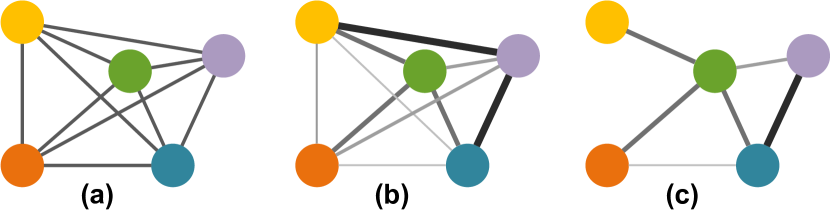
Figure 1: The current methods to infer latent graphs in MARL can be categorized into three types: (a) fully connected unweighted graphs, (b) fully connected weighted graphs, and (c) sparse weighted graphs. These methods rely solely on one-step observations, leading to deficient graphs that foster redundant or detrimental information exchanges and suffer from high computational complexity for action-pair calculations.

While these methods balance computational efficiency with effective agent interaction and complex decision-making, in the real world, agents should not only consider their own observations but also take into account the situations of others when taking action [7]. Effective cooperation among agents emerges as a pivotal factor in achieving specific objectives. This cooperation can be assumed to have some latent graph structures [8]. Since the graph is not explicitly given, the inference of meaningful dynamic graph topology has been a persistent challenge.

The current methods to address this problem can be broadly categorized into three types, illustrated in Fig.1. The first type involves employing fully connected unweighted graphs, such as PIC [9] and DCG [10]. The second type incorporates fully connected weighted graphs, such as GraphMIX [11] and DICG[12]. The third type utilizes weighted sparse graphs, such as SOP-CG [13] and CASEC [14]. However, these methods exhibit the following limitations: (1) They primarily focus on one-step observations and fail to consider the value of historical trajectory data, which more accurately represents agents’ behaviours and is more meaningful to help to learn policies [15]. This overreliance on one-step data can lead to suboptimal graph learning, producing graphs that may encourage redundant or even counterproductive information exchanges, thereby impeding effective policy learning. (2) The computation-intensive nature of action-pair calculations in coordination graphs (CG) [8] poses significant scalability challenges, especially in fully-connected settings. For instance, in a system with $N$ agents, each having $A$ actions, the computational complexity of these methods is $O(A^{2}N^{2})$. This complexity becomes increasingly problematic as the number of agents and actions increases.

In this paper, we address these limitations by proposing a novel approach called Latent Temporal Sparse Coordination Graph (LTS-CG) for MARL. LTS-CG efficiently infers graphs using agents’ observation trajectories to generate an agent-pair probability matrix, where the probability is absorbed and trained together with Graph Convolutional Networks (GNN) parameters. The computational complexity of this procedure scales quadratically with the number of agents $N$, which renders our approach scalable and suitable for handling complex MARL scenarios. Subsequently, a sparse graph is sampled from this matrix, which simultaneously captures agent dependencies underlying the trajectories and models the relation-uncertainty between agents. Driven by the goal of creating meaningful graphs, we enhance agents’ understanding of their peers and the environment by embedding two essential characteristics into the graph: Predict-Future and Infer-Present. Predict-Future empowers agents to predict upcoming observations using current observations and the sampled graph, providing valuable insights for immediate decision-making. Infer-Present aids each partially observed agent in comprehending the full environmental context and deducing the current state with the graph’s information. LTS-CG leverages both historical and real-time data for graph training, considering local and global perspectives. The temporal structure of the learned graph encapsulates past experiences, with edge weights reflecting ongoing observations. This facilitates knowledge exchange during policy learning and supports historical and present insights for effective cooperation. The computational complexity of our method is $O(TN^{2})$, where $T$ represents the observation length used for graph learning, making it more efficient than action-pair-based methods.

The main insight behind designing our method is to enable simultaneous graph inference and multi-agent policy learning, facilitating efficient end-to-end training using standard policy optimization methods. We evaluate LTS-CG on the StarCraft II benchmark, demonstrating its superior performance. The ablation results empirically proved that using trajectories for learning the coordination graph is more effective than relying on one-step observations, and having the Predict-Future and Infer-Present characteristics improves the performance of LTS-CG. The contributions of this paper are summarized as follows:

• We pioneer the treatment of agent trajectories as data streams in MARL with LTS-CG. Our method leverages these trajectories to infer latent temporal sparse graphs, facilitating knowledge exchange between agents.

• By sampling sparse graphs from trajectories-generated agent probability matrices, LTS-CG captures agent dependencies and models the uncertainty of relations between agents simultaneously, with computational complexity only related to the number of agents.

• LTS-CG further infers the graph from both local and global standpoints to encode Predict-Future and Infer-Present characteristics. This meaningful graph enables agents to gain historical and present perspectives to achieve effective cooperation.

The rest of the paper is organized as follows. In Sec. II, we give a definition of our task, followed the related work in Sec. III. In Sec. IV, we described our approach. We report experimental studies in Sec. V and conclude in Sec. VI.

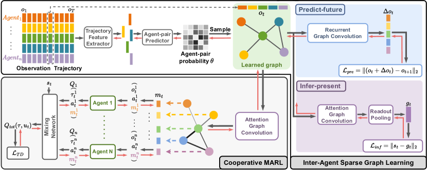
Figure 2: The framework of LTS-CG. LTS-CG samples a sparse graph from an agent-pair probability matrix generated by agents’ observation trajectories. We further learn the graph to encode two essential characteristics: Predict-Future enables agents to predict future steps effectively, and Infer-Present empowers every partially observed agent to deduce the current state using graph information. The learned temporal graph structure captures past experiences, while current observations determine edge weights. This allows agents to exchange knowledge during policy learning and gain historical and present perspectives for effective cooperation. Graph learning and agent training occur simultaneously in an end-to-end fashion.

II Preliminaries

We focus on cooperative multi-agent tasks modelled as a Decentralized Partially Observable Markov Decision Process (Dec-POMDP) [16] consisting of a tuple $\langle\mathcal{I},\mathcal{S},\{\mathcal{A}^{i}\}_{i=1}^{n},P,\{\mathcal{O}^{i}\}_{i=1}^{n},\{\sigma^{i}\}_{i=1}^{n},R,\gamma\rangle$, where $\mathcal{I}$ is the finite set of $n$ agents, $s\in\mathcal{S}$ is the true state of the environment. At each time step, each agent $i$ observes the state partially by drawing observation $o^{i}_{t}\in\mathcal{O}^{i}$ and selects an action $a^{i}_{t}\in\mathcal{A}^{i}$ according to its own policy $\sigma^{i}$. Individual actions form a joint action $\boldsymbol{a}=(a_{1},...,a_{n})$, which leads to the next state $s^{\prime}$ according to the transition function $P(s^{\prime}|s,\boldsymbol{a})$ and a reward $R(s,\boldsymbol{a})$ shared by all agents. Each agent has local action-observation history $\tau_{i,t}=(o_{i,0},a_{i,0},...,o_{i,t-1},a_{i,t-1},o_{i,t})\in(\mathcal{O}^{i}\times\mathcal{A}^{i})^{t}\times\mathcal{O}^{i}$. This paper considers episodic tasks yielding episodes $(s_{0},\{o^{i}_{0}\}_{i=1}^{n},\boldsymbol{a}_{0},r_{0},...,s_{T},\{o^{i}_{T}\}_{i=1}^{n})$ of varying finite length $T$. Agents learn to collectively maximize the global return $Q_{tot}(s,\boldsymbol{a})=\mathbb{E}_{s_{0:T},a_{0:T}}\left[\sum_{t=0}^{T}\gamma^{t}R\left(s_{t},\boldsymbol{a}_{t}\right)\mid s_{0}=s,\boldsymbol{a}_{0}=\boldsymbol{a}\right]$, where $\gamma\in[0,1)$ is the discount factor.

Learning the underlying relation of agents can be seen as the inference of a meaningful dynamic graph topology. This graph is denoted as $\mathcal{G}=\{\mathcal{V},\mathcal{E}\}$ where $\mathcal{V}=\mathcal{I}$ is node/agent set and $\mathcal{E}$ is the edge/relation set between agents.

III Related Work

III-A Graph-based MARL

MARL faces the challenge of dealing with the exponentially growing size of joint action spaces among agents [17]. The paradigm of CTDE [18, 19] strikes a balance between computational efficiency and multi-agent interaction but falls short in handling dependencies between agents. Graph Neural Networks (GNNs) have demonstrated remarkable capability in modelling relational dependencies [20, 21], making graphs a compelling tool for graph-based MARL, which can be generally divided into two types. One type involves using graphs as coordination graphs during policy training, such as DCG [10], SOP-CG [13] and CASEC [14]. In this approach, the total action-value function is defined as:

$$Q_{tot}\!\left(s_{t},\boldsymbol{a}\right)\!=\!\frac{1}{|\mathcal{V}|}\sum_{i\in\mathcal{V}}q^{i}\left(a^{i}\!\mid\!s_{t}\right)\!+\!\frac{1}{|\mathcal{E}|}\!\sum_{\{i,j\}\in\mathcal{E}}\!\!\!q^{ij}\!\left(a^{i},a^{j}\!\mid\!s_{t}\right),$$ (1)

where the first term calculates the Q-value of each action (also known as utility function), and the second term evaluates every action-pair of agents (also known as payoff function). This method explicitly assesses the quality of joint actions between different agents. The other type uses graphs to facilitate information exchange among agents, such as DICG [22] and G2ANet [23]. It is formulated as:

$$m_{i}=\text{AGG}_{j\in\mathcal{N}_{i}}(f(o_{j},a_{j})),\quad Q_{tot}=\sum_{i=1}^{n}Q_{i}(o_{i},a_{i},m_{i})$$ (2)

where $\mathcal{N}_{i}$ means the neighbours of agent $i$. $f(\cdot)$ transfers the original observation and action into embedding, and AGG($\cdot$) aggregates the embedding based on graph topology to generate the message $m_{i}$. This message provides additional knowledge that aids agents in decision-making and represents an implicit coordination between agents. Although these methods do not strictly calculate the payoff-utility function based on the coordination graph, they build upon the same idea of reasoning about joint actions based on interactions between agents [22].

As the graph itself is not explicitly given, inferring graph topology remains a critical prerequisite for training MARL. From the perspective of graph structure, existing methods for graph inference can be broadly categorized into three types: (a) creating fully connected unweighted graphs by directly linking all nodes/agents explicitly, such as DGN [24], PIC [9] and DCG [10] or implicitly such as MAAC [25], ROMA [26]; (b) employing attention mechanisms to calculate fully connected weighted graphs, such as GraphMIX [11] and DICG [12]; (c) designing drop-edge criteria to generate sparse weighted graphs, such as random drop edges in G2ANet [21], select sparse graph from candidate set in SOP-CG [13] and drop edges based on variance of payoff functions in CASEC [14].

Despite this progress, these methods exhibit the following limitations: one is that they primarily focus on one-step observations and fail to consider the value of historical trajectory data, which more accurately represents agents’ behaviours and is more meaningful to help to learn policies [15]; another is that the computation-intensive nature of action-pair calculations in coordination graphs (CG) [8] poses significant scalability challenges, which becomes increasingly problematic as the number of agents and actions increases (See: V-A).

III-B Graph Structure Learning

To learn a relational graph between agents that take a series of actions within specific time steps, two promising directions are worth considering: learning a graph for multiple time series forecasting and inferring a graph for trajectory prediction. For the former, Yu et al. [27] explored pairwise similarities or connections among them to enhance forecasting accuracy. Wu et al. [28] presented a framework for modelling multivariate time series data and learning graph structures that can be used with or without a pre-defined graph structure. Satorras et al. [29] proposed an approach that balances accuracy and computational efficiency, allowing the flexibility to infer either fully connected or bipartite graphs. Regarding trajectory prediction, Kipf et al. [30] proposed NRI, a variational autoencoder that leverages a latent-variable approach to learn a latent graph. On the other hand, LDS [31] and GTS [32] focus on learning probabilistic graph models by optimizing performance over the graph distribution mean. To further adaptively connect multiple nodes, Li et al. [33] proposed a group-aware relational reasoning approach to infer hyperedges. In the context of MARL, the absence of labelled data poses a challenge for traditional trajectory prediction or multiple time series forecasting methods. Borrowing the learning capabilities from these two directions while fully leveraging the information available in MARL remains an underexplored area.

IV The Proposed Method

The framework of LTS-CG is illustrated in Fig. 2. To efficiently infer the underlying relation from past experiences, LTS-CG samples a sparse graph from the agent-pair probability matrix generated by agents’ observation trajectories. The core of LTS-CG lies in creating a meaningful graph that enhances agents’ understanding of their peers and the environment. This is achieved through two key characteristics: Predict-Future and Infer-Present, which enable agents to share knowledge and gain both historical and present insights, fostering effective cooperation. Detailed descriptions of each component are provided in the subsequent sections.

IV-A Latent Temporal Sparse Graphs Learning

IV-A1 Sparse graph construction

The accumulated observation trajectories of all agents encapsulate their experiences of interactions with the environment and their cooperation. To efficiently capture the underlying relationships, instead of directly learning the structure of the inter-agent sparse graph $A$, we utilize observation trajectories $\{\mathcal{O}^{i}\}_{i=1}^{n}$ to generate the agent-pair probability matrix $\theta\in[0,1]^{n\times n}$. This matrix parameterizes the element-wise Bernoulli distribution [31], which allows us to sample a graph representing the relevant connections between agents. This graph learning objective is achieved by minimizing the loss of function

$$\min_{w}\quad\mathrm{E}_{A\sim\operatorname{Ber}(\theta(w))}\left[\mathcal{L}\left(A,w,\mathcal{O}_{T}\right)\right].$$ (3)

Here, $\mathcal{O}_{T}=\{{\mathcal{O}^{i}_{T}\}_{i=1}^{n}}$, and $\mathcal{O}^{i}_{T}=\{o^{i}_{0},...,o^{i}_{T}\}$ denotes the observation trajectory for agent $i$ over the time steps $T$. Each element of $A$ is sampled from a Bernoulli distribution $\operatorname{Ber}(\theta(w))$, with $\omega$ denoting the trainable weight. In Eq. (3), the adjacent probability $\theta$ is absorbed together with the GNNs parameters $w$, making the gradient computation more efficient and having better scalability [32]. In the following, we give the details about how to infer the inter-agent sparse graph $A$ and how to define the graph learning loss function $\mathcal{L}$.

To acquire knowledge about the temporal dependence of each agent and the relationship between agents, we establish the observation experience extractor $f_{oe}(\cdot)$ to help us capture the temporal dependence of each agent $z^{i}$ by employing convolution along the time dimension, followed by a fully connected layer, defined as

$$z^{i}=f_{oe}(\mathcal{O}^{i}_{T})=\text{FC}(\text{CONV}(\mathcal{O}^{i}_{T})),$$ (4)

where $\text{FC}(\cdot)$ is a fully connected layer and $\text{CONV}(\cdot)$ is the convolution layer performed along the temporal dimension. This convolutional layer plays a crucial role in capturing each agent’s latent behaviour patterns over time, enhancing the model’s ability to discern dynamic and temporal patterns in the agents’ interactions. Then the agent-pair predictor $f_{ap}(\cdot)$ utilize the temporal dependencies of every agent-pair ($z^{i}$ and $z^{j}$) to calculate adjacent probability $\theta_{ij}$ as follows

$$\theta_{ij}=f_{ap}(z^{i}\|z^{j})=\text{FC}(\text{FC}(z^{i}\|z^{j})),$$ (5)

where $\|$ denotes concatenation along the feature dimension. We adopt multi-layer perceptrons (MLPs) to model and learn $f_{ap}(\cdot)$, leveraging the universal approximation theorem [34] to enhance their representational capacity.

To enable backpropagation through the Bernoulli sampling, we apply the Gumbel parameterization trick [35, 36]. This technique leverages the properties of the Gumbel distribution to approximate the sampling process in a differentiable manner, allowing gradients to flow through the stochastic operation. In the context of Bernoulli sampling, the Gumbel trick involves generating two Gumbel-distributed random variables, denoted as $g_{ij}^{1}$ and $g_{ij}^{2}$, for each element $A_{ij}$ in the adjacency matrix. These random variables are sampled from a Gumbel distribution with a location parameter of 0 and a scale parameter of 1. The sampled values from the Gumbel distribution are then used to compute the logits for the sigmoid function in the Bernoulli sampling equation. Specifically, the logits are calculated as:

$$A_{ij}\!=\operatorname{sigmoid}\left(\left(\log\left(\theta_{ij}/\!\left(1\!-\!\theta_{ij}\right)\right)\!+\!\left(g_{ij}^{1}\!-\!g_{ij}^{2}\right)\right)\!/s\right),$$ (6)

where $g_{ij}^{1},g_{ij}^{2}\sim\operatorname{Gumbel}(0,1)$ for all $i,j$, $\theta_{ij}$ represents the probability parameter for the Bernoulli distribution, and $s$ is a temperature parameter that controls the sharpness of the sampling process. As the temperature $s\rightarrow 0,A_{ij}=1$ with probability $\theta_{ij}$ and 0 with remaining probability. By applying Eq. (5) and Eq. (6), we convert the observation trajectories $\mathcal{O}_{T}$ into an agent-pair probability $\theta$. We subsequently sample to obtain the inter-agent graph $A$ for further learning and utilization in cooperative MARL.

IV-A2 Meaningful graph learning

Motivated by the idea that the graph should enhance the agents’ understanding of other agents and the environment, we further learn the graph to encode the following two essential characteristics.

Predict-Future means by exploiting the graph, we aim to empower agents to predict future steps effectively, enabling them to make better decisions in the current time step. We use the diffusion convolutional gated recurrent unit introduced in Diffusion Convolutional Recurrent Neural Network (DCRNN) [37] and leverage the learned graphs $A$ to process the observations of all agents $\mathcal{O}_{t}={\{o^{i}_{t}\}_{i=1}^{n}}$ as follows

$$\begin{array}[]{ll}&R_{t}=\operatorname{sigmoid}\left(W_{R}\star_{A}\left[\mathcal{O}_{t}\|H_{t-1}\right]+b_{R}\right),\\ &C_{t}=\tanh\left(W_{C}\star_{A}\left[\mathcal{O}_{t}\|\left(R_{t}\odot H_{t-1}\right]+b_{C}\right)\right.\\ &U_{t}=\operatorname{sigmoid}\left(W_{U}\star_{A}\left[\mathcal{O}_{t}\|H_{t-1}\right]+b_{U}\right),\\ &H_{t}=U_{t}\odot H_{t-1}+\left(1-U_{t}\right)\odot C_{t},\end{array}$$ (7)

where the graph convolution $\star_{A}$ is defined as

$$W_{Q}\star_{A}Y=\sum_{k=0}^{K}\left(w_{k,1}^{Q}\left(D_{O}^{-1}A\right)^{k}+w_{k,2}^{Q}\left(D_{I}^{-1}A^{T}\right)^{k}\right)Y,$$ (8)

with $D_{O}$ and $D_{I}$ being the out-degree and in-degree matrix of learned agent-pair matrix $A$, respectively. Here, $w_{k,1}^{Q},w_{k,2}^{Q},b_{Q}$ for $Q=R,U,C$ are model parameters and $K$ is the diffusion degree. We adopt a $1$-layer DCRNN and set $K=3$ in our experiments.

To capture both temporal and spatial dependencies between agents, we feed a $T$-step observations ${\{o^{i}_{t+1:t+T}\}_{i=1}^{n}}$ into Eq.(7), to forecast the future changes in the current $T$-step observation. The output of the hidden state in every step represents the prediction of how the current observation will change in the next step, denoted as $H_{t+1:t+T}={\{\Delta o^{i}_{t+1:t+T}\}_{i=1}^{n}}$. Then, the Predict-Future is achieved by calculating the following loss function

$$\mathcal{L}_{pre}=\sum_{i}^{n}\sum_{t^{\prime}=1}^{T}\left\|\left(o^{i}_{t+t^{\prime}}+\Delta o^{i}_{t+t^{\prime}}\right)-o^{i}_{t+1+t^{\prime}}\right\|_{2}.$$ (9)

Since Eq. (9) is calculated by the observation of each agent, Predict-Future is a local-level characteristic of LTS-CG. Employing the message-passing mechanism of GNNs [38], it enables agents to predict future observations based on their own current observations and the passed information from neighbouring agents.

Infer-Present is designed to assist every partially observed agent in gaining the ability to grasp the entire environmental context and deduce the current state with the information provided by the graph. Given the current observation ${\{o^{i}_{t}\}_{i=1}^{n}}$, we first generate the observation embeddings matrix $E_{t}=[e_{t}^{1\top},...,e_{t}^{n\top}]$ using the ongoing observation extractor $e_{t}^{i}=f_{obs}(o_{t}^{i})$, where $f_{obs}$ is a MLPs. Then we adopt an attention mechanism to dynamically calculate the edge weight between every pair of agents resulting in the attention edge-weight matrix, defined as

$$\mu_{t}^{ij}=\frac{\text{exp}(e_{t}^{j\top}W_{a}e_{t}^{i})}{\sum_{k\in\mathcal{N}_{i}}\text{exp}(e_{t}^{k\top}W_{a}e_{t}^{i})},\quad C_{t}^{ij}=\mu_{t}^{ij},$$ (10)

where $\mathcal{N}_{i}$ represents the neighbors of agent $i$ in the graph and $W_{a}$ is trainable parameter of attention mechanism. The weighted-agent-pair matrix is updated as $A_{t}^{\prime}=C_{t}A$, and the graph convolution [39] is performed using the following equation

$$H_{t}^{l}=ReLU\Big{(}\hat{A}_{t}H_{t}^{(l-1)}W^{(l-1)}\Big{)},$$ (11)

where $l$ is the index of GNN layers, $\hat{A}_{t}=\tilde{D}^{-\frac{1}{2}}A^{\prime}_{t}\tilde{D}^{-\frac{1}{2}}$, $\tilde{D}_{ii}=\sum_{j}A^{\prime}_{t}[i,j]$, and $H_{t}^{0}=E_{t}$ . The current sparse graph $A_{t}^{\prime}$ not only encapsulates historical information within its structure but also captures the ongoing agent relationships through the edge weights. The message-passing mechanism of the GNN in Eq.(11) enables agents to exchange their knowledge effectively at every time step. The current feature of the entire graph at the $t$-step is defined as

$$g_{t}=\text{READOUT}(\sum_{i}^{N}H_{t}[i,:]),$$ (12)

where $\text{READOUT}(\cdot)$ is an average function aggregating all the agents’ information to obtain the entire graph feature. The Infer-Present is achieved by

$$\mathcal{L}_{inf}=\sum_{t=1}^{T}\left\|g_{t}-s_{t}\right\|_{2},$$ (13)

where $s_{t}$ denotes the actual state of the environment at the $t$ step. Infer-Present is a global-level characteristic of LTS-CG that utilizes graph convolution to facilitate a seamless exchange of observations among agents, allowing the entire graph (comprising all agents/nodes and their relationships/edges) to represent the current state of the environment collectively.

With the above two characters, the generalized loss function for the graph learning Eq.(3) now can be formalized as

$$\mathcal{L}\left(A,w,\mathcal{O}_{T}\right)=\mathcal{L}_{g}=\mathcal{L}_{pre}+\mathcal{L}_{inf}.$$ (14)

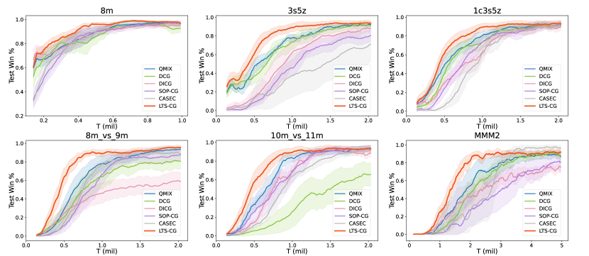
Figure 3: Performance of our method and baselines on six maps of the StarCraft II benchmark [40]. Y-axis is the test winning rate of the game. X-axis is training steps

IV-B Cooperative MARL with LTS-CG

In our design, LTS-CG facilitates simultaneous graph inference and multi-agent policy learning for efficient end-to-end training. Initially, with the buffer’s setup, we store the inter-agent graph with full connectivity. This allows agents to start the game with the capability to cooperate and make decisions. As training progresses, LTS-CG dynamically learns and updates the graph’s structure within the buffer. During testing, the graph, retrieved from the buffer, is updated with edge weights based on current observations. This temporal sparse graph is then utilized for message calculation and dissemination, ensuring agents have access to the latest information. Such an approach guarantees effective decision-making and cooperation throughout the training process.

Leveraging the learned graph $A$ at every time step and following the Eq.(10), the current observation ${\{o^{i}_{t}\}_{i=1}^{n}}$ are used to compute the edge weights in $A$. These edge weights determine the importance of cooperating with neighbouring agents. Consequently, we obtain the latent temporal sparse coordination graph, encompassing historical information within its structure and ongoing agent relationships through its edge weights. The exchanged knowledge $m_{i}=H_{t}^{l}[i,:]$ between agents is then shared on this graph. Using Eq.(11), what information should be exchanged is calculated during cooperation. This process enhances the agents’ perception, prediction, and decision-making capabilities. With this knowledge, the local action-value function is defined as $Q_{i}(\tau_{i},a_{i},m_{i})$. To keep the balance of computational efficiency with effective agent interaction and complex decision-making, we build our algorithm on top of the QMIX [5] to integrate all the individual Q values. The total-action value is monotonic in the per-agent values, which is formulated as

$$\underset{\mathbf{a}}{\operatorname{argmax}}Q_{tot}(\boldsymbol{\tau},\mathbf{a})=\left(\begin{array}[]{c}\operatorname{argmax}_{a_{1}}Q_{1}\left(\tau_{1},a_{1},m_{1}\right)\\ \vdots\\ \operatorname{argmax}_{a_{n}}Q_{n}\left(\tau_{n},a_{n},m_{n}\right)\end{array}\right).$$ (15)

The entire framework is trained by minimizing the loss function

$$\mathcal{L}(\boldsymbol{\theta})=\mathcal{L}_{TD}(\boldsymbol{\theta}^{-})+\lambda\mathcal{L}_{g}\left(\boldsymbol{\theta}_{g}\right),$$ (16)

where $\boldsymbol{\theta}$ includes all parameters in the model, $\mathcal{L}_{g}$ represents the graph loss from Eq. (14) and $\lambda$ is the weight of graph loss. The TD loss $\mathcal{L}_{TD}(\boldsymbol{\theta}^{-})$ in Eq. (16) is defined as

$$\mathcal{L}_{TD}(\boldsymbol{\theta}^{-})\!=\!\left[r\!+\!\gamma\max_{\boldsymbol{a}^{\prime}}Q_{tot}\left(s^{\prime},\boldsymbol{a}^{\prime};\boldsymbol{\theta}^{\prime}\right)\!-\!Q_{tot}(s,\boldsymbol{a};\boldsymbol{\theta}^{-})\right]^{2},$$ (17)

where $\boldsymbol{\theta}^{\prime}$ denotes the parameters of a periodically updated target network, as commonly employed in DQN. By training with the Eq. (16), our method enables simultaneous graph inference and multi-agent policy learning, facilitating efficient end-to-end training using standard policy optimization methods.

V Experiments

In this section, we design experiments to answer the following questions: (1) How does LTS-CG compare in performance with state-of-the-art methods on complex cooperative multi-agent tasks? (See: V-A) (2) Is the utilization of trajectories for learning the coordination graph more effective than relying on one-step observations? (See: V-B1) (3) Does having the Predict-Future and Infer-Present characteristics improve the performance of LTS-CG? (See: V-B2) (4) What are the effects of varying the weights for $\mathcal{L}_{g}$ on the experimental outcomes? (See: V-B3)

To answer the above questions, we conduct our experiments on StarCraft II benchmark [40], which consists of different maps with varying numbers of agents. The experiments included scenarios with a minimum of eight agents, comprising both homogeneous and heterogeneous agent setups. All the experiments are carried out with difficulty=7 and repeated with 5 random seeds. We employ distinct 2-layer GNNs as specified in Eq.(11) to facilitate the acquisition of the Infer-present characteristic and to compute the knowledge exchanged during agents’ cooperation. The graph loss $\lambda$, the character-balance weight $b$ and $c$ in Eq (16) are set to 1. The hyperparameters used for MARL in StarCraft II are given in Tab. II. Experiences are stored in a first-in-first-out (FIFO) replay buffer and during the training phase. The experiments are finished with Intel(R) Xeon(R) E-2288G CPU and Tesla V100-PCIE-32GB GPU. The software that we use for experiments is Python 3.7.13, PyTorch 1.13.1, PyYAML 6.0, numpy 1.21.5 and CUDA 11.6.

Maps	Agent Num.	Enemy Num.	Action Num.	Episode Limit
8m	8	8	14	120
25m	25	25	31	150
3s5z	8	8	14	150
1c3s5z	9	9	15	180
8m_vs_9m	8	9	15	120
10m_vs_11m	10	11	17	150
27m_vs_30m	27	30	36	180
MMM2	10	12	18	180

TABLE I: Detailed information of each map we used in StarCraft II benchmark.

Hyperparameter	Value
Batch-size	32
Replay memory size	5000
discount factor $\gamma$	0.99
Optimizer	RMSProp
Learning rate	$5\times 10^{-4}$
optim_alpha	0.99
optim_eps	$1\times 10^{-5}$
Gradient-norm-clip	10
Action-selector	$\epsilon$-greedy
$\epsilon$-start	1.0
$\epsilon$-finish	0.05
$\epsilon$-anneal-time	50000 steps
target update interval	200

TABLE II: The hyperparameters used in StarCraft II.

Method	Graph type	Edge	Data in learning graph
QMIX	$\times$	$\times$	$\times$
DCG	Complete	Unweighted	One-step
DICG	Complete	Weighted	One-step
SOP-CG	Sparse	Unweighted	One-step
CASEC	Sparse	Weighted	One-step
LTS-CG	Sparse	Weighted	Trajectories

TABLE III: Comparison of different experiment methods in terms of graph type, edge representation, and data used for learning graph.

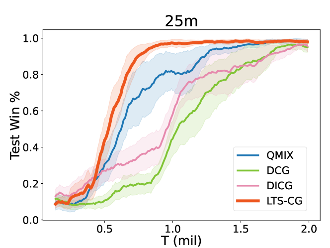
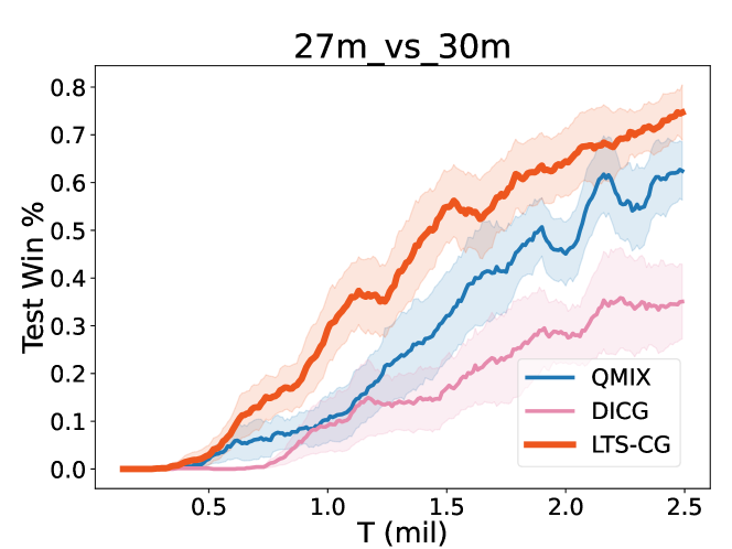
Figure 4: Performance comparison on the 25m and 27m_vs_30m maps. Due to the high computational complexity, SOP-CG and CASEC could not complete the experiments on both maps. DCG could not finish the experiment on the later map.

V-A Performance comparison on StarCraft II

V-A1 Details for comprised methods

We utilize several state-of-the-art baseline algorithms for our experiments. Each method’s graph type, edge representation, and group utilization are summarised in Tab. III. Below, we provide a brief introduction of each method and the detailed settings we used:

• QMIX [5] is effective but without cooperation between agents. We adopt the configuration specified in the StarCraft Multi-Agent Challenge [40] for the QMIX algorithm.

• DCG [10] directly links all the agents to get an unweighted fully connected graph. The graph is used to calculate the action-pair values function. For DCG, we employ a low-rank payoff approximation with $K=1$ (as described in Eq.(5) of the original paper) and incorporate privileged information through the action representation learning technique. This corresponds to the DCG-S (rank 1) setting outlined in the original paper.

• DICG [12] uses attention mechanisms to calculate weighted fully connected graph. The graph is used to pass information between agents. We utilize the DICG algorithm in the context of the centralised training centralised execution (CTCE) paradigm. This approach involves using QMIX as the base policy learning framework. The graph learning procedure strictly follows the DICG methodology.

• SOP-CG [13] selects sparse graphs from a pre-calculated candidate set. In line with the original paper, we adopt the tree organization $\mathcal{G}_{T}$ for SOP-CG. In this configuration, the agents are organized in a tree structure with $n-1$ edges, ensuring that all agents form a connected component.

• CASEC [14] drops some edges on the weighted fully connected graph according to the variance payoff function. We employ the construction_q_var (Eq.(4) in the paper) and q_var_loss (Eq. 8 in the paper) strategies described in the original paper. The weight of the sparseness loss term is set to $\lambda_{sparse}=0.3$ in our experiments.

V-A2 Results

Fig. 3 presents the results of our method compared to the performance of other algorithms on six different maps. The experimental results clearly demonstrate the superiority of our approach LTS-CG across all scenarios (shown in orange). Firstly, our method exhibited faster convergence than the compared methods on all six maps in the early stages of training (below 0.6 mil for 8m, 2 mil for MMM2, and 1 mil for other maps). This indicates that our approach enables the agents to quickly learn effective cooperative strategies and achieve high-performance levels. Moreover, our method demonstrated a smaller standard deviation in performance compared to the other methods, such as CASEC in 3s5z, DICG in 8m_vs_9m and DCG in 10m_vs_11m. The reduced variability suggests that our approach consistently produces reliable and stable cooperative behaviours, resulting in more predictable and robust performance across different maps. Notably, our method achieved consistent and competitive performance across all six maps. This indicates that our approach generalizes well and is capable of adapting to various environmental conditions and agent configurations. The ability to achieve good results consistently is essential for real-world applications of multi-agent systems.

Comparing our method to two SOTA approaches, SOP-CG and CASEC, which aim to learn sparse graphs for MARL, we observed interesting patterns in their performance on specific maps. In the 3s5z, 1c3s5z, and 10m_vs_11m maps, SOP-CG outperformed CASEC. However, in the 8m_vs_9m and MMM2 maps, CASEC exhibited superior performance compared to SOP-CG. The varying performance of SOP-CG and CASEC indicates the importance of learning the meaningful graph based on the environment and agent setup, which further highlights the advantages of our approach in achieving constant and competitive performance across diverse scenarios.

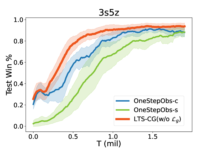
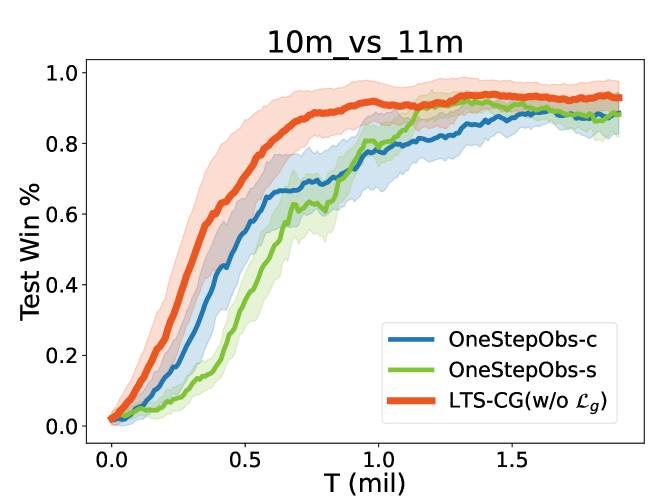
Figure 5: Performance comparison on the 3s5z and 10m_vs_11m. OneStepObs-c and OneStepObs-s utilize a one-step observation to generate a fully connected graph and a sparse graph separately. LTS-CG$(w/o\mathcal{L}_{g})$ investigates the effectiveness of using trajectories by omitting the Predict-Future and Infer-Present characteristics.

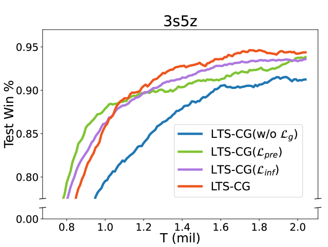
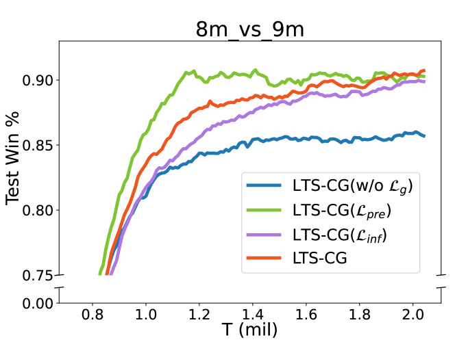
Figure 6: Evaluate the effectiveness of the different latent temporal sparse graph learning strategies on two maps. LTS-CG$(w/o\mathcal{L}g)$ excludes both Predict-Future and Infer-Present characteristics. LTS-CG$(\mathcal{L}{pre})$ and LTS-CG$(\mathcal{L}_{inf})$ only incorporate the Predict-Future or Infer-Present characteristic into the learning process separately.

Large maps. We further investigated the performance of the proposed method on larger maps: 25m and 27m_vs_30m, which are designed to test the scalability and efficiency of the algorithms under high computational complexity. Due to the high computational demands in representing action-pairs, two SOTA approaches, SOP-CG and CASEC, could not complete the experiments on both maps, and DCG could not finish the experiment on the 27_vs_30m map, which is indicative of their computational limitations in this context. In Fig. 4, the results of our proposed method on these two maps were presented. Our approach demonstrated promising performance compared to the other methods, even in these challenging and computationally intensive scenarios. Notably, the QMIX algorithm (shown in blue), which operates without explicit cooperation mechanisms or coordination graphs, surprisingly outperforms DCG and DICG (shown in light green and pink, respectively), which are graph-based learning algorithms. This result indicates that while the graph-based approaches are designed to foster coordination among agents, the lack of a well-constructed coordination graph can be detrimental, potentially hindering the policy learning process.

In summary, the experiments suggest that graph-based coordination in multi-agent settings must be carefully crafted to ensure that it is conducive to the learning environment. The results highlight the necessity for well-designed graph structures that enhance rather than impede policy learning, as evidenced by the success of LTS-CG in complex scenarios where other graph-based methods struggle.

V-B Ablation study

V-B1 Trajectory Graph Learning vs One-Step Observations

We examined the effect of graph generation methods on MARL performance in the 3s5z and 10m_vs_11m scenarios. We considered three settings:

• OneStepObs-c generates a fully connected graph using one-step observations, akin to methods like DICG [12].

• OneStepObs-s employs one-step observations to create a sparse graph, similar to G2ANet [21].

• LTS-CG$(w/o\mathcal{L}_{g})$ utilizes trajectories for graph generation while excluding Predict-Future and Infer-Present characteristics to solely assess the impact of trajectory-based learning.

As depicted in Fig. 5, LTS-CG$(w/o\mathcal{L}_{g})$ surpasses both OneStepObs-c and OneStepObs-s in win percentage over training iterations, demonstrating its superior performance in cooperative multi-agent settings. This finding underscores the significant benefit of trajectory-based graph generation in enhancing MARL performance, independent of other factors. The shaded areas in the figure represent the variance across multiple runs, with LTS-CG$(w/o\mathcal{L}_{g})$ not only achieving higher win rates but also exhibiting less variance, reflecting its consistent and reliable performance.

Furthermore, in Fig. 5, the comparison among LTS-CG$(w/o\mathcal{L}_{g})$, OneStepObs-c (a method similar to DICG), and OneStepObs-s (a method similar to G2ANet) shows that LTS-CG$(w/o\mathcal{L}_{g})$ demonstrates the most significant performance improvement in terms of win percentage across training iterations. This outcome highlights the advantages of using trajectory-based information for graph generation, even without relying on specialized characteristics like Predict-Future and Infer-Present.

The shaded regions in the graph represent the variance in win percentages over multiple runs, providing insights into the reliability of the methods. Notably, LTS-CG$(w/o\mathcal{L}_{g})$ achieves higher win rates and maintains tighter confidence intervals, suggesting a consistent performance advantage over the other methods. These experimental results provide strong support for the hypothesis that trajectory-based graph learning is more effective and robust than one-step observation-based methods, contributing significantly to the advancement of cooperative multi-agent learning techniques.

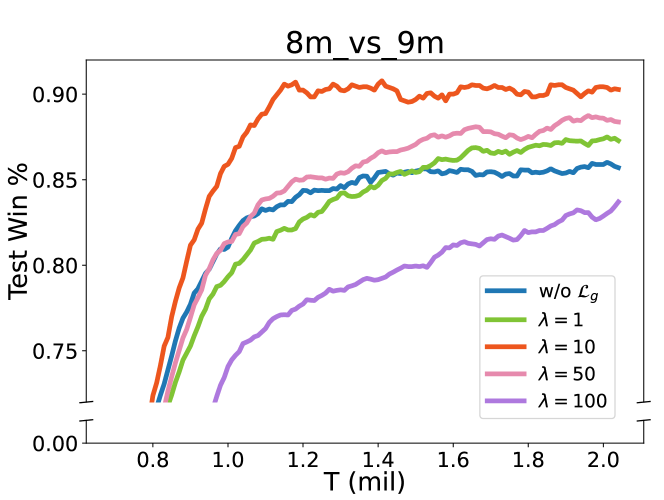
Figure 7: Evaluate the effect of the different weights of graph loss.

V-B2 Latent Temporal Sparse Graph Learning strategies

We conducted an evaluation to assess the effectiveness of different strategies and examine the importance of the Predict-Future and Infer-Present characteristics in graph learning. Our investigation focused on the following settings:

• LTS-CG$(w/o\mathcal{L}_{g})$ excludes both Predict-Future and Infer-Present characteristics. This setting implies that we do not further refine the learned graph structure after sampling.

• LTS-CG$(\mathcal{L}_{pre})$ only incorporates the Predict-Future characteristic into the learning process.

• LTS-CG$(\mathcal{L}_{inf})$ only incorporates the Infer-Present characteristic into the learning process.

• LTS-CG with both Predict-Future and Infer-Present characteristics, where we consider both aspects simultaneously.

The final performance is assessed on the 8m_vs_9m, and 3s5z maps and the results are presented in Fig. 6. The ablation study revealed several important findings. Firstly, regardless of whether we include the Predict-Future, the Infer-Present, or both characteristics, the performance was consistently better than not having anyone. This highlights the importance of having these characteristics in enhancing the learning of the inter-agent graph and improving cooperative behaviour. Moreover, on the 8m_vs_9m map, with the Predict-Future characteristic outperformed the other settings. One possible reason for this observation is that the agents in this map are homogeneous, sharing similar characteristics. Knowing the next time observation benefits the overall cooperation among the agents. In contrast, in the 3s5z map agents are heterogeneous. Utilizing observations from different agents to infer the current state proves beneficial for learning in this scenario. Although using both characteristics simultaneously introduces more parameters and slightly slower convergence, promising results are obtained after approximately 2 million time steps, showcasing the effectiveness of leveraging both characteristics for improved cooperative multi-agent learning. This ablation study confirms the significance of two characteristics in LTS-CG for learning meaningful graphs to help agents cooperate.

V-B3 Weight of graph loss

We tested the different weight of graph loss $\mathcal{L}_{g}$ on two maps, as shown in Fig. 7. $(w/o\text{ }\mathcal{L}_{g})$ represents the scenario where the MARL training does not include the graph loss term, i.e., $\lambda=0$. The results demonstrate the positive impact of incorporating $\mathcal{L}_{g}$ in MARL, as compared to the case without it. Specifically, when $\mathcal{L}_{g}=1,10,50$, the addition of $\mathcal{L}_{g}$ Consistently improves the performance of MARL on both maps. As the value of $\lambda$ increases, the final results during training on both maps first improve and then start to decline, which indicates that the weight $\lambda$ of the graph loss function has a noticeable influence on the final results. We present empirical evidence related to the parameter $\lambda$ here.

Identifying the most appropriate $\lambda$ value for specific scenarios is a labour-intensive task that requires additional experimentation. It involves balancing leveraging the benefits of graph-based learning and avoiding potential overfitting or performance degradation due to excessive emphasis on the graph loss term. This process underscores the nuanced nature of parameter tuning in MARL and highlights the need for careful consideration when designing and optimizing such systems.

V-C Discussion

In this discussion, we underscore the contrasts between our proposed approach and CG-based methods (e.g., DCG [10], SOP-CG [13], and CASEC [14]), as well as with the method where the graph serves for information exchange (e.g., DICG [12], G2ANet [21]).

	$1m$ steps time $(h)$	Time Complexity
DCG	$11.63\pm 0.64$	$O(A^{2}N^{2})$
SOP-CG	$19.46\pm 0.80$	$O(A^{2}N^{2})$
CASEC	$10.12\pm 0.51$	$O(A^{2}N^{2})$
LTS-CG	$8.84\pm 0.49$	$O(TN^{2})$

TABLE IV: Time consumption on map 10m_vs_11m and complexity analysis with CG-based methods.

V-C1 Coordination graphs (CG) methods

The CG is denoted as $\mathcal{G}=\{\mathcal{V},\mathcal{E}\}$ where $\mathcal{V}$ is agent/node set and $\mathcal{E}$ is the edge set between agents [8, 41]. These CG-based methods factorize the Q-function into utility functions $q^{i}$ and payoff functions $q^{ij}$ as follows:

$$Q_{tot}\!\left(s_{t},\boldsymbol{a}\right)\!=\!\frac{1}{|\mathcal{V}|}\sum_{i\in\mathcal{V}}q^{i}\left(a^{i}\!\mid\!s_{t}\right)\!+\!\frac{1}{|\mathcal{E}|}\!\sum_{\{i,j\}\in\mathcal{E}}\!\!\!q^{ij}\!\left(a^{i},a^{j}\!\mid\!s_{t}\right).$$ (18)

However, due to the large number of action pairs represented by the payoff functions $q^{ij}$, these methods face challenges of high computational complexity. To alleviate this concern, various approaches have been employed, such as low-rank approximation in DCG [10], construction of polynomial-time CG in SOP-CG [13], and dropping edges using variance payoff functions in CASEC [14]. Despite these efforts, the inherent high complexity of CG-based methods, as high as $O(A^{2}N^{2})$, limits their applicability in large-scale scenarios.

By contrast, the complexities of LTS-CG is $O(TN^{2})$, where $N$ is the number of agents, and $T$ is the length of trajectories. For instance, consider experiments conducted on the map 10m_vs_11m, involving 10 agents and 17 actions, resulting in 289 potential action-pair within $q^{ij}$. Table IV illustrates the time requirements of various methods, revealing that CG-based approaches demand more time to complete $1m$ time steps than our method. Particularly noteworthy is the significantly higher time consumption of SOP-CG and the remarkably elevated GPU usage of CASEC (25.85 GB), contrasted with DCG (2.29 GB), SOP-CG (4.00 GB), and our approach (4.13 GB). Moreover, it’s important to highlight that all CG-based methods failed to conclude the experiment on the 27_vs_30m map, involving the calculation of $36^{2}=1296$ action-pair for every two agents (the complexity now is $O(1296\times N^{2})$). In contrast, for our proposed LTS-CG method, even though we set the length of trajectory for graph learning to the episode limit, the computational complexity remains a modest $O(180\times N^{2})$. In the actual experiment, this trajectory length typically falls below the episode limit. Thus, LTS-CG delivers competitive performance while maintaining a reasonable level of computational efficiency.

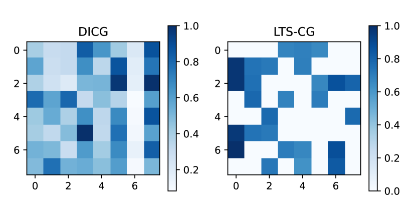
Figure 8: Visualization of latent agent-pair matrices learned by DICG and LTS-CG on map 8m_vs_9m.

V-C2 Graphs for information exchange

Current methods using graphs for information exchange rely on attention mechanisms to calculate edge weight. Like DICG [12], these methods learn a weighted fully-connected graph, which inevitably transfers redundant or even detrimental information between agents, as illustrated in Fig.8. This drawback impedes individual agents’ capacity to acquire effective policies. In contrast, our method generates a sparser graph focusing on the most relevant relationships among agents, leading to more efficient and effective cooperation.

Another existing method is G2ANet [21], which uses both hard and soft attention to generate a sparse graph for MARL. However, our method offers two distinct advantages over G2ANet: (1) G2ANet focuses solely on ongoing information, while we leverage the complete observation trajectories to capture the latent relationships between agents, shown in Sec.V-B1. (2) Unlike G2ANet’s arbitrary edge reduction using the attention mechanism, our approach harnesses agents’ experience and current information to acquire a meaningful graph. This graph exhibits two critical attributes, the efficacy of which has been demonstrated through Sec.V-B2.

VI Conclusions and Future directions

This paper introduces LTS-CG, a novel approach for MARL that infers a latent temporal sparse graph to enable effective information exchange among agents. To efficiently infer the graph from past experiences, LTS-CG uses the agents’ observation trajectories to generate the agent-pair probability matrix. Motivated by the idea that the meaningful graph should enrich agents’ comprehension of their peers and the environment, we further learn the graph to encode two essential characteristics: Predict-Future and Infer-Present. The former is a local-level characteristic that gives agents valuable insights into the future environment, enhancing their decision-making capabilities in the current time step. The latter is a global-level one that enables partially observed agents to deduce the current state, promoting overall cooperation among agents. By having them, LTS-CG learns temporal graphs from historical and real-time information, facilitating knowledge exchange during policy learning and effective collaboration. Graph learning and agent training occur simultaneously in an end-to-end manner. Experimental evaluations on the StarCraft II benchmark demonstrate the superior performance of our method over existing ones.

For future directions, it is imperative to extend the scope of graph learning beyond agent-pair relationships. Investigating higher-order relationships, such as group dynamics, while inferring cooperation graphs can deepen our understanding of cooperative behaviours among agents. Additionally, addressing the challenges posed by asynchronous scenarios is crucial. Developing techniques to effectively learn cooperation graphs in such scenarios will enhance the applicability and robustness of methods in real-world environments.

References

- Wang et al. [2022a] M. Wang, L. Wu, J. Li, and L. He, “Traffic signal control with reinforcement learning based on region-aware cooperative strategy,” IEEE Trans. Intell. Transp. Syst., vol. 23, no. 7, pp. 6774–6785, 2022.
- Rizk et al. [2019] Y. Rizk, M. Awad, and E. W. Tunstel, “Cooperative heterogeneous multi-robot systems: A survey,” ACM Comput. Surv., vol. 52, no. 2, pp. 29:1–29:31, 2019.
- Cui et al. [2020] J. Cui, Y. Liu, and A. Nallanathan, “Multi-agent reinforcement learning-based resource allocation for UAV networks,” IEEE Trans. Wirel. Commun., vol. 19, no. 2, pp. 729–743, 2020.
- Sunehag et al. [2018] P. Sunehag, G. Lever, A. Gruslys, W. M. Czarnecki, V. F. Zambaldi, M. Jaderberg, M. Lanctot, N. Sonnerat, J. Z. Leibo, K. Tuyls, and T. Graepel, “Value-decomposition networks for cooperative multi-agent learning based on team reward,” in the 17th International Conference on Autonomous Agents and MultiAgent Systems (AAMAS 2018), Stockholm, Sweden, 2018, pp. 2085–2087.
- Rashid et al. [2018] T. Rashid, M. Samvelyan, C. S. de Witt, G. Farquhar, J. N. Foerster, and S. Whiteson, “QMIX: monotonic value function factorisation for deep multi-agent reinforcement learning,” in the 35th International Conference on Machine Learning (ICML 2018), Stockholmsmässan, Stockholm, Sweden, vol. 80, 2018, pp. 4292–4301.
- Son et al. [2019] K. Son, D. Kim, W. J. Kang, D. Hostallero, and Y. Yi, “QTRAN: learning to factorize with transformation for cooperative multi-agent reinforcement learning,” in the 36th International Conference on Machine Learning (ICML 2019), Long Beach, California, USA, vol. 97, 2019, pp. 5887–5896.
- Hong et al. [2022] Y. Hong, Y. Jin, and Y. Tang, “Rethinking individual global max in cooperative multi-agent reinforcement learning,” in the 36th Annual Conference on Neural Information Processing Systems (NIPS 2022), vol. 35, 2022, pp. 32 438–32 449.
- Guestrin et al. [2002a] C. Guestrin, M. G. Lagoudakis, and R. Parr, “Coordinated reinforcement learning,” in the 19th International Conference (ICML 2002), University of New South Wales, Sydney, Australia, 2002, pp. 227–234.
- Liu et al. [2020a] I.-J. Liu, R. A. Yeh, and A. G. Schwing, “Pic: Permutation invariant critic for multi-agent deep reinforcement learning,” in the 3rd Conference on Robot Learning (CoRL 2019), Osaka, Japan, vol. 100, 2020, pp. 590–602.
- Boehmer et al. [2020] W. Boehmer, V. Kurin, and S. Whiteson, “Deep coordination graphs,” in the 37th International Conference on Machine Learning (ICML 2020), Virtual Event, vol. 119, 2020, pp. 980–991.
- Naderializadeh et al. [2020] N. Naderializadeh, F. H. Hung, S. Soleyman, and D. Khosla, “Graph convolutional value decomposition in multi-agent reinforcement learning,” CoRR, vol. abs/2010.04740, 2020.
- Li et al. [2021] S. Li, J. K. Gupta, P. Morales, R. E. Allen, and M. J. Kochenderfer, “Deep implicit coordination graphs for multi-agent reinforcement learning,” in the 20th International Conference on Autonomous Agents and Multiagent Systems (AAMAS 2021), Virtual Event, United Kingdom, 2021, pp. 764–772.
- Yang et al. [2022] Q. Yang, W. Dong, Z. Ren, J. Wang, T. Wang, and C. Zhang, “Self-organized polynomial-time coordination graphs,” in International Conference on Machine Learning (ICML 2022), Baltimore, Maryland, USA, vol. 162, 2022, pp. 24 963–24 979.
- Wang et al. [2022b] T. Wang, L. Zeng, W. Dong, Q. Yang, Y. Yu, and C. Zhang, “Context-aware sparse deep coordination graphs,” in the 10th International Conference on Learning Representations (ICLR 2022), Virtual Event, 2022.
- Pacchiano et al. [2020] A. Pacchiano, J. Parker-Holder, Y. Tang, K. Choromanski, A. Choromanska, and M. Jordan, “Learning to score behaviors for guided policy optimization,” in the 37th International Conference on Machine Learning, (ICML 2020), vol. 119, 13–18 Jul 2020, pp. 7445–7454.
- Oliehoek and Amato [2016] F. A. Oliehoek and C. Amato, A Concise Introduction to Decentralized POMDPs, ser. Springer Briefs in Intelligent Systems. Springer, 2016.
- Oroojlooy and Hajinezhad [2023] A. Oroojlooy and D. Hajinezhad, “A review of cooperative multi-agent deep reinforcement learning,” Appl. Intell., vol. 53, no. 11, pp. 13 677–13 722, 2023.
- Lowe et al. [2017] R. Lowe, Y. Wu, A. Tamar, J. Harb, P. Abbeel, and I. Mordatch, “Multi-agent actor-critic for mixed cooperative-competitive environments,” in the 30th Annual Conference on Neural Information Processing Systems (NIPS 2017), Long Beach, CA, USA, 2017, pp. 6379–6390.
- Foerster et al. [2018] J. N. Foerster, G. Farquhar, T. Afouras, N. Nardelli, and S. Whiteson, “Counterfactual multi-agent policy gradients,” in the 32nd AAAI Conference on Artificial Intelligence (AAAI 2018), New Orleans, Louisiana, USA, 2018, pp. 2974–2982.
- Wu et al. [2021] Z. Wu, S. Pan, F. Chen, G. Long, C. Zhang, and P. S. Yu, “A comprehensive survey on graph neural networks,” IEEE Trans. Neural Networks Learn. Syst., vol. 32, no. 1, pp. 4–24, 2021.
- Liu et al. [2020b] Y. Liu, W. Wang, Y. Hu, J. Hao, X. Chen, and Y. Gao, “Multi-agent game abstraction via graph attention neural network,” in the 34th AAAI Conference on Artificial Intelligence (AAAI 2020), New York, NY, USA,, 2020, pp. 7211–7218.
- Wang et al. [2020a] T. Wang, J. Wang, C. Zheng, and C. Zhang, “Learning nearly decomposable value functions via communication minimization,” in the 8th International Conference on Learning Representations (ICLR 2020), Addis Ababa, Ethiopia, 2020.
- Duan et al. [2022] W. Duan, J. Xuan, M. Qiao, and J. Lu, “Learning from the dark: Boosting graph convolutional neural networks with diverse negative samples,” in the 36th AAAI Conference on Artificial Intelligence (AAAI 2022), Virtual Event. AAAI Press, 2022, pp. 6550–6558.
- Jiang et al. [2020] J. Jiang, C. Dun, T. Huang, and Z. Lu, “Graph convolutional reinforcement learning,” in 8th International Conference on Learning Representations (ICLR 2020), Addis Ababa, Ethiopia, 2020.
- Iqbal and Sha [2019] S. Iqbal and F. Sha, “Actor-attention-critic for multi-agent reinforcement learning,” in the 36th International Conference on Machine Learning (ICML 2019), Long Beach, California, USA, vol. 97, 2019, pp. 2961–2970.
- Wang et al. [2020b] T. Wang, H. Dong, V. R. Lesser, and C. Zhang, “ROMA: multi-agent reinforcement learning with emergent roles,” in the 37th International Conference on Machine Learning (ICML 2020), Virtual Event, vol. 119, 2020, pp. 9876–9886.
- Yu et al. [2018] B. Yu, H. Yin, and Z. Zhu, “Spatio-temporal graph convolutional networks: A deep learning framework for traffic forecasting,” in the 27th International Joint Conference on Artificial Intelligence (IJCAI 2018), Stockholm, Sweden, 2018, pp. 3634–3640.
- Wu et al. [2020] Z. Wu, S. Pan, G. Long, J. Jiang, X. Chang, and C. Zhang, “Connecting the dots: Multivariate time series forecasting with graph neural networks,” in The 26th ACM SIGKDD Conference on Knowledge Discovery and Data Mining (KDD 2020), Virtual Event, CA, USA, 2020, pp. 753–763.
- Satorras et al. [2022] V. G. Satorras, S. S. Rangapuram, and T. Januschowski, “Multivariate time series forecasting with latent graph inference,” CoRR, vol. abs/2203.03423, 2022.
- Kipf et al. [2018] T. N. Kipf, E. Fetaya, K. Wang, M. Welling, and R. S. Zemel, “Neural relational inference for interacting systems,” in the 35th International Conference on Machine Learning (ICML 2018), Stockholmsmässan, Stockholm, Sweden, vol. 80. PMLR, 2018, pp. 2693–2702.
- Franceschi et al. [2019] L. Franceschi, M. Niepert, M. Pontil, and X. He, “Learning discrete structures for graph neural networks,” in the 36th International Conference on Machine Learning (ICML 2019), Long Beach, California, USA, vol. 97, 2019, pp. 1972–1982.
- Shang et al. [2021] C. Shang, J. Chen, and J. Bi, “Discrete graph structure learning for forecasting multiple time series,” in the 9th International Conference on Learning Representations (ICLR 2021), Virtual Event, Austria, 2021.
- Li et al. [2022] J. Li, C. Hua, J. Park, H. Ma, V. M. Dax, and M. J. Kochenderfer, “Evolvehypergraph: Group-aware dynamic relational reasoning for trajectory prediction,” CoRR, vol. abs/2208.05470, 2022.
- Hornik [1991] K. Hornik, “Approximation capabilities of multilayer feedforward networks,” Neural Networks, vol. 4, no. 2, pp. 251–257, 1991.
- Jang et al. [2017] E. Jang, S. Gu, and B. Poole, “Categorical reparameterization with gumbel-softmax,” in the 5th International Conference on Learning Representations (ICLR 2017), Toulon, France, 2017.
- Maddison et al. [2017] C. J. Maddison, A. Mnih, and Y. W. Teh, “The concrete distribution: A continuous relaxation of discrete random variables,” in the 5th International Conference on Learning Representations (ICLR 2017),Toulon, France, 2017.
- Li et al. [2018] Y. Li, R. Yu, C. Shahabi, and Y. Liu, “Diffusion convolutional recurrent neural network: Data-driven traffic forecasting,” in the 6th International Conference on Learning Representations (ICLR 2018), Vancouver, BC, Canada, 2018.
- Duan et al. [2024] W. Duan, J. Lu, Y. G. Wang, and J. Xuan, “Layer-diverse negative sampling for graph neural networks,” Transactions on Machine Learning Research, 2024.
- Kipf and Welling [2017] T. N. Kipf and M. Welling, “Semi-supervised classification with graph convolutional networks,” in the 5th International Conference on Learning Representations (ICLR 2017), Toulon, France, April 24-26, 2017.
- Samvelyan et al. [2019] M. Samvelyan, T. Rashid, C. S. de Witt, G. Farquhar, N. Nardelli, T. G. J. Rudner, C. Hung, P. H. S. Torr, J. N. Foerster, and S. Whiteson, “The starcraft multi-agent challenge,” in the 18th International Conference on Autonomous Agents and MultiAgent Systems (AAMAS 2019), Montreal, QC, Canada,, 2019, pp. 2186–2188.
- Guestrin et al. [2002b] C. Guestrin, S. Venkataraman, and D. Koller, “Context-specific multiagent coordination and planning with factored mdps,” in the 18th National Conference on Artificial Intelligence, (AAAI 2002), 2002, pp. 253–259.