Sine Activated Low-Rank Matrices for Parameter Efficient Learning

Abstract

Low-rank decomposition has emerged as a vital tool for enhancing parameter efficiency in neural network architectures, gaining traction across diverse applications in machine learning. These techniques significantly lower the number of parameters, striking a balance between compactness and performance. However, a common challenge has been the compromise between parameter efficiency and the accuracy of the model, where reduced parameters often lead to diminished accuracy compared to their full-rank counterparts. In this work, we propose a novel theoretical framework that integrates a sinusoidal function within the low-rank decomposition process. This approach not only preserves the benefits of the parameter efficiency characteristic of low-rank methods but also increases the decomposition’s rank, thereby enhancing model accuracy. Our method proves to be an adaptable enhancement for existing low-rank models, as evidenced by its successful application in Vision Transformers (ViT), Large Language Models (LLMs), Neural Radiance Fields (NeRF), and 3D shape modeling. This demonstrates the wide-ranging potential and efficiency of our proposed technique.

1 Introduction

In the last few years, large-scale machine learning models have shown remarkable capabilities across various domains, achieving groundbreaking results in tasks related to vision and natural language processing. However, these models come with a significant drawback: their training necessitates an extensive memory footprint. This challenge has spurred the demand for more compact, parameter-efficient architectures. A prominent solution that has emerged is the use of low-rank techniques, which involve substituting the large, dense matrices in large-scale models with smaller, low-rank matrices. This substitution not only simplifies the models but also shifts the computational complexity from quadratic to linear, making a significant impact on efficiency. In the context of high-capacity models like Vision Transformers (ViTs) and Large Language Models (LLMs) that utilize millions to billions of parameters, transitioning from dense to low-rank matrices can result in considerable cost savings. Nonetheless, adopting low-rank architectures does introduce a trade-off, as they typically do not achieve the same level of accuracy as their full-rank counterparts, presenting a balance between parameter efficiency and model performance.

Addressing this challenge, our work unveils a novel technique that retains the parameter efficiency intrinsic to low-rank methods while achieving superior accuracy. Our method hinges on the realization that augmenting a low-rank matrix with a high-frequency sinusoidal function can elevate its rank without inflating its parameter count. We lay out a theoretical framework elucidating why and how such sinusoidal modulation crucially enhances the matrix’s rank. By utilizing this non-linearity into low-rank decompositions, we design compact architectures that not only maintain their streamlined nature but also deliver improved accuracy across various machine learning tasks.

An example of this insight is depicted in the left image of Fig. 1, revealing the singular value spectra of low-rank versus full-rank matrices in comparison to our sinusoidally enhanced matrix. This enhancement allows our matrix to more closely resemble the spectrum of a full-rank matrix, without an increase in parameters, laying the foundation for our model’s improved accuracy. Further validation of our architecture’s performance is demonstrated in the right image of Fig. 1, which compares three ViT architectures on the ImageNet-1K dataset. Here, our model maintains the same parameter efficiency as the low-rank version yet achieves a performance boost of 3-4% underscoring its superior efficacy.

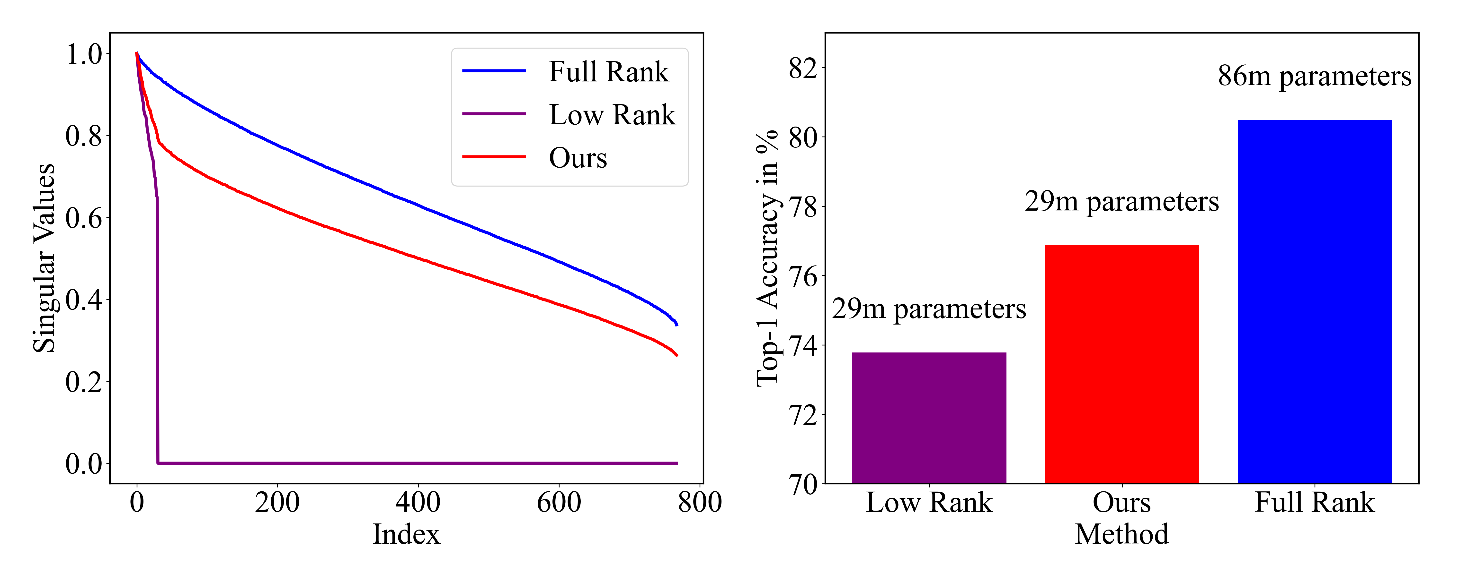
Figure 1: In this figure, we illustrate the impact of low-rank approximation and our sine activated low-rank method on the weight matrix spectrum and performance in the ViT-Base model’s Feed-Forward Network. All singular values are normalized to 1. The left part shows the SVD spectrum for matrices initialized with the Kaiming uniform method: full-rank, low-rank, and sine activated low-rank matrices. On the right, we note that while low-rank approximation reduces parameter count, it also lowers performance. Our sine activated low-rank approach can improve the accuracy by approximately 4% without increasing the parameter count.

Our approach’s inherited advantages are further corroborated across a range of machine learning applications, including variations of ViT, Low-Rank Adaptation (LoRA) methods for LLMs, Neural Radiance Fields (NeRF) for novel view synthesis, and 3D shape modeling via binary occupancy fields. Across the board, our approach not only matches the parameter savings offered by low-rank methods but also secures an improvement in accuracy, attesting to its broad applicability and superior performance. The main contributions of our paper are:

• A parameter-efficient matrix decomposition that rivals traditional low-rank decompositions in terms of parameter economy while delivering enhanced accuracy.

• A comprehensive theoretical framework that substantiates our approach, providing a solid underpinning for our methodology.

• Extensive empirical validation has been conducted across a diverse set of applications, each demonstrating our model’s superior accuracy and effectiveness.

2 Related Work

2.0.1 Low-rank decomposition:

stands as a crucial method across disciplines like information theory, optimization, and machine learning, providing a strategic approach to reduce memory costs [32, 38]. Notably, [3] uncovered that matrices can precisely separate low-rank and sparse components through convex programming, linking to matrix completion and recovery. Expanding its application, [40] devised a low-rank learning framework for Convolutional Neural Networks, enhancing compression while maintaining accuracy. [30] further found that performance improvements in Large Language Models could be achieved by eliminating higher-order weight matrix components without extra parameters or data. In the realm of neural radiance fields, [34] introduced a rank-residual learning strategy for optimal low-rank approximations, facilitating model size adjustments. Additional contributions include [31] with rank-constrained distillation, [5] applying vector-matrix decomposition, and [29] using soft-gated low-rank decompositions for compression. More recently, [41] implemented a vector-matrix decomposition strategy that allows for test-time compression adjustments.

2.0.2 Parameter efficient learning:

is an important research area in deep learning, merging various techniques to enhance model adaptability with minimal resource demands [22]. Techniques like parameter-efficient fine-tuning (PEFT) allow pre-trained models to adjust to new tasks efficiently, addressing the challenges of fine-tuning large models due to high hardware and storage costs. Among these, Visual Prompt Tuning (VPT) stands out for its minimal parameter alteration—less than 1%—in the input space, effectively refining large Transformer models while keeping the core architecture unchanged [18]. Similarly, BitFit offers a sparse-finetuning approach, tweaking only the model’s bias terms for cost-effective adaptations [42]. Moreover, LoRA introduces a low-rank adaptation that maintains model quality without additional inference latency or altering input sequence lengths, by embedding trainable rank matrices within the Transformer layers [17]. Recent studies also combine LoRA with other efficiency strategies like quantization, pruning, and random projections for further model compression [8, 21, 43, 19]

3 Methodology

In this section, we introduce our technique which we term a sine activated low-rank matrix. The main purpose of this technique is to increase the rank of an initial low-rank matrix without adding parameters.

3.1 Notation

3.1.1 Feed-Forward Layer

Our technique is defined for feed-forward layers of a neural architecture. In this section, we fix the notation for such layers. We will express a feed-forward layer as

$$\mathbf{y}=\mathbf{W}\mathbf{x}+\mathbf{b}$$ (1)

where $\mathbf{W}\,{\in}\,\mathbb{R}^{m{\times}n}$ is a dense weight matrix, $\mathbf{b}\,{\in}\,\mathbb{R}^{m{\times}1}$ is the bias of the layer, and $\mathbf{x}$ is the input from the previous layer. The output $\mathbf{y}$ is then often activated by a non-linearity $\sigma$ producing $\sigma(\mathbf{y})$. The weight matrix $\mathbf{W}$ and bias $\mathbf{b}$ are trainable parameters of the layer. In contemporary deep learning models, the feed-forward layers’ weight matrices, $\mathbf{W}$, are often large and dense yielding a high rank matrix. While the high-rank property of the weight matrix helps in representing complex signals, it significantly adds to the overall parameter count within the network yielding the need for a trade-off between the rank of the weight matrix and overall architecture capacity.

3.1.2 Low-rank decomposition

A full-rank weight matrix $\mathbf{W}$ can be replaced by low-rank matrices $\mathbf{U}\mathbf{V}^{T}$, such that $\mathbf{W}\,{=}\,\mathbf{U}\mathbf{V}^{T}$, where $\mathbf{U}\in\mathbb{R}^{m{\times}k},\mathbf{V}\,{\in}\,\mathbb{R}^{n{\times}k}$ and $k\,{\ll}\,min(m,n)$.

$$\mathbf{y}=\mathbf{W}\mathbf{x}+\mathbf{b}=(\mathbf{U}\mathbf{V}^{T})\mathbf{x}+\mathbf{b}\\$$ (2)

This is the most common way to reduce the parameter count in the feed-forward layer. During the training process, this method performs optimization on $\mathbf{U}$ and $\mathbf{V}$ alternatively. Low-rank multiplication then reduces the learnable parameter count and memory footprint rom $O(mn)$ to $O(k\cdot(m{+}n))$. Although $\mathbf{U}\mathbf{V}^{T}$ has the same matrix shape as the full-rank matrix $\mathbf{W}$, the rank of $\mathbf{U}\mathbf{V}^{T}$ is constrained and $rank(\mathbf{U}\mathbf{V}^{T})\,{\leq}\,r$. Thus while we have significantly decreased the number of trainable weights in such a layer, we have paid the price by obtaining a matrix of much smaller rank. In the next section, we address this trade-off by developing a technique that can raise back the rank of a low-rank decomposition while keeping its low parameter count.

3.2 Theoretical Framework

In this subsection, we formally describe the simple design of the naive low-rank method and our proposed Sine Activated Low-Rank method. The principles outlined here apply to any dense layers in deep learning models.

3.2.1 Non-linearity low-rank decomposition

We introduce non-linearity transformation into low-rank matrices.

$$\mathbf{y}=\frac{\phi(\omega\cdot\mathbf{U}\mathbf{V}^{T})}{g}\mathbf{x}+\mathbf{b}$$ (3)

where $\phi(\cdot)$ is the non-linearity function, $\omega$ is a non-learnable frequency parameter, and $g$ is a non-learnable parameter to adjust the gain of the transformation.

3.2.2 Main theorem:

In this section, we provide a theoretical framework that clearly shows how to increase the rank of a low-rank decomposition without adding any parameters. We will show that if we choose the non-linearity, in the decomposition defined in Sec. 3.2.1, to be a sine function then provided the frequency $\omega$ is chosen high enough, the rank of the matrix $\phi(\omega\,{\cdot}\,\mathbf{U}\mathbf{V}^{T})$ will be larger than that of $\mathbf{UV}^{T}$. The proofs of the theorems are given in the supp. material. To begin with, we fix $\omega\,{>}\,0$ and let $\sin(\omega\,{\cdot}\,\mathbf{A})$ denote the matrix obtained from a fixed $m{\times}n$ matrix $\mathbf{A}$ by applying the function $\sin(\omega\,{\cdot}\,\mathbf{x})$ component-wise to $\mathbf{A}$. Assuming $\mathbf{A}\,{\neq}\,0$ we define $A_{\min}^{0}$ as:

$$A_{\min}^{0}=\min_{i,js.t.A_{ij\neq 0}}|A_{ij}|.$$ (4)

Note that such a quantity is well defined precisely because $\mathbf{A}$ has a finite number of entries and all such entries cannot be zero from the assumption that $\mathbf{A}\,{\neq}\,0$.

The following theorem relates the rank of $\sin(\omega\,{\cdot}\,\mathbf{A})$ to the frequency parameters $\omega$ and the quantity $A_{\min}^{0}$.

Proposition 1

Fix an $m{\times}n$ matrix $\mathbf{A}$ s.t. $\mathbf{A}\,{\neq}\,0$. Then

$$Rank(\sin(\omega\cdot\mathbf{A}))\geq\omega\bigg{(}\frac{A_{\min}^{0}}{||\sqrt{|\mathbf{A}|}||_{op}}\bigg{)}^{2}\text{ if }0\leq\omega\leq\frac{\pi}{3A^{0}_{\min}}$$ (5)

Prop. 1 shows that if we modulate the matrix $\sin(\omega\,{\cdot}\,\mathbf{A})$ by increasing $\omega\,{>}\,0$ then the rank of the matrix $\sin(\omega\,{\cdot}\,\mathbf{A})$ can be increased provided $\omega\,{<}\,\frac{\pi}{3A^{0}_{\min}}$. We can apply Prop. 1 to the context of a low-rank decomposition as defined in Sec. 3.1.2. Given a low-rank decomposition $\mathbf{UV}^{T}$ with $\mathbf{U}\,{\in}\,\mathbb{R}^{m{\times}k}$ and $\mathbf{V}\,{\in}\,\mathbb{R}^{n{\times}k}$ with $k\,{\ll}\,\min\{m,n\}$ the following theorem shows how we can increase the rank of the decomposition by applying a $\sin(\omega\cdot)$ function.

Theorem 3.1

Let $\mathbf{U}\,{\in}\,\mathbb{R}^{m{\times}k}$ and $\mathbf{V}\,{\in}\,\mathbb{R}^{n{\times}k}$ with $k\,{\ll}\,\min\{m,n\}$. Assume both $\mathbf{U}$ and $\mathbf{V}$ are initialized according to a uniform distribution $\mathcal{U}(-1/N,1/N)$ where $N\,{>}\,k$. Then there exists an $\omega_{0}$ such that the matrix $\sin(\omega\,{\cdot}\,\mathbf{A})$ will satisfy the inequality

$$Rank(\sin(\omega\,{\cdot}\,\mathbf{UV}^{T}))\,{>}\,Rank(\mathbf{UV}^{T})$$ (6)

provided $\omega\,{\geq}\,\omega_{0}$.

We mention that Thm. 3.1 also holds for the case where we initialize $\mathbf{U}$ and $\mathbf{V}$ by a normal distribution of variance $N$.

Weight matrices within feed-forward layers are typically initialized using a distribution that is contingent upon the layer’s neuron count. When considering low-rank decompositions characterized by matrices $\mathbf{U}\,{\in}\,\mathbb{R}^{m{\times}k}$ and $\mathbf{V}^{T}\,{\in}\,\mathbb{R}^{k{\times}n}$, where $k\,{\ll}\,\min\{m,n\}$, the variance of this initialization distribution is influenced by $m$ and $n$. These dimensions are significantly larger than $k$, ensuring that the condition specified in Thm. 3.1—that $N\,{>}\,k$—is nearly always met, making this theorem especially relevant for low-rank decompositions in feedforward layers. For example the most common initialization schemes such as Kaiming [15] and Xavier [12] satisfy the requirements of our theorem.

Thm. 3.1 offers a viable strategy for maintaining a high-rank characteristic in feed-forward layers while simultaneously minimizing the parameter count. By introducing a sinusoidal non-linearity with a sufficiently high frequency $\omega$ into a low-rank decomposition, it is possible to elevate the rank without altering the quantity of trainable parameters. This key insight from our theoretical analysis aims to highlight a novel approach to optimizing network structure for enhanced computational efficiency and model performance.

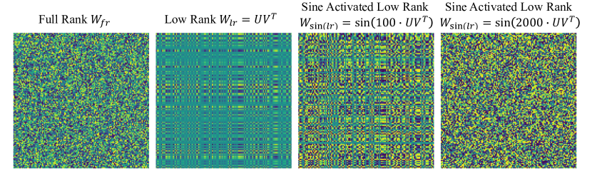
Figure 2: These figures display weight magnitudes for matrices with dimension $128{\times}128$. The first figure showcases a heatmap of a full-rank matrix initialized by the Kaiming uniform, highlighting linear independence among rows. The second shows a low-rank matrix $\mathbf{W_{\text{lr}}}\,{=}\,\mathbf{UV}^{T}\,{\in}\,\mathbb{R}^{128{\times}128}$, with $\mathbf{U},\mathbf{V}\,{\in}\,\mathbb{R}^{128{\times}1}$ initialized by Kaiming uniform illustrating minimal linear independence. The final pair of figures reveal how applying a sine function element-wise, $\sin(\omega\,{\cdot}\,\mathbf{UV}^{T})$, with varying $\omega$, affects linear independence in low-rank matrices; specifically, $\omega\,{=}\,100$ and $\omega\,{=}\,2000$ progressively increase linear independence and thus visually showing such a strategy increases the rank.

In Fig. 2, we give a visualization of our method in action. We consider a full-rank matrix, a low-rank matrix, and two sine activated low-rank matrices with different frequencies. By visualizing the weight magnitudes in each matrix via a heat map, we can clearly see how the sine activated low-rank matrix increases rank and furthermore how increasing the frequency of the sine function increases the rank in accord with Thm. 3.1.

Building upon Eq. 3, we explore the application of various non-linear functions to a low-rank decomposition, with a particular focus on the sine function. This choice is inspired by Thm. 3.1, which theoretically demonstrates that applying a sine function effectively increases the matrix rank. In Fig. 3 (left), we present a comparative analysis of the sine function against other common non-linear functions in machine learning, such as the sigmoid and ReLU. The results clearly illustrate that the sine function increases the rank, making it an optimal non-linearity to apply to a low-rank decomposition.

Further, Thm. 3.1 suggests that augmenting the frequency of the sine function applied to a low-rank decomposition contributes to a further increase in rank. To empirically validate this, we conducted experiments applying sine functions of various frequencies to a constant low-rank matrix. The outcomes, depicted in Fig. 3 (right), corroborate the theorem’s prediction, showcasing a positive correlation between the frequency of the sine function and the resultant rank increase.

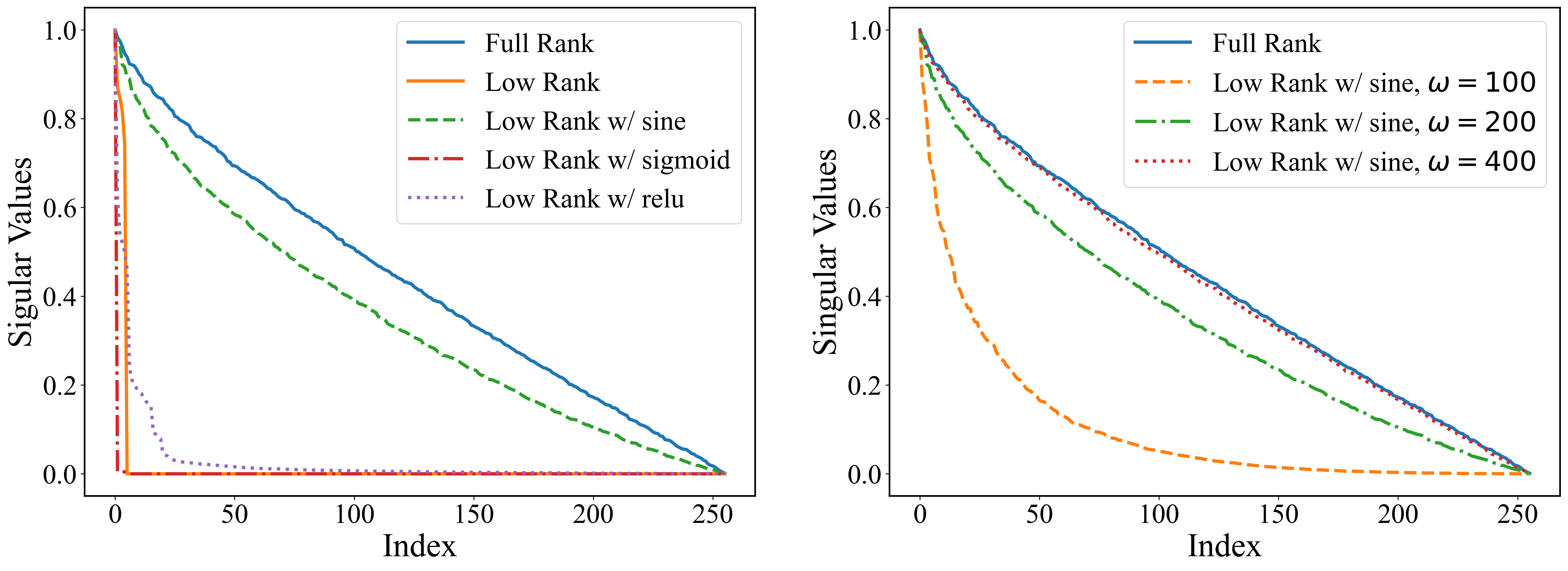
Figure 3: In this figure we depict the SVD spectrum of a Kaiming uniform initialized matrix $\mathbf{W_{\text{fr}}}\in\mathbb{R}^{256\times 256}$ and a low-rank $k=5$ approximation matrix $\mathbf{W_{\text{lr}}}=\mathbf{U}\mathbf{V}^{T}$, where $\mathbf{U},\mathbf{V}\in\mathbb{R}^{256\times 5}$ are initialized using Kaiming uniform [15]. All singular values are normalized to 1. On the left we depict the spectral advantages of applying a non-linear function $\phi(\omega\cdot\mathbf{U}\mathbf{V}^{T})$ where $\omega$ is a hyper-parameter. Here we see the natural advantages of the sine function such that $\phi(\mathbf{x})=\sin(\omega\cdot\mathbf{x})$. On the right, we demonstrate empirically how manipulating $\omega$ within the sine function can change these spectral properties.

4 Experiments

This section is dedicated to validating and analyzing the efficacy of our proposed low-rank methods across a spectrum of neural network architectures. To demonstrate the broad applicability and versatility of our approach, we examine its performance in three distinct contemporary applications. Specifically, we explore its integration into the pretraining of Vision Transformers (ViT)[10], the reconstruction of scenes using neural radiance fields (NeRF)[25], the fine-tuning of large language models through low-rank adaptation (LoRA) [17], and the 3D shape modeling. This collectively underscores our model’s adaptability to a diverse array of low-rank frameworks, highlighting its potential to significantly impact various domains within the field of computer vision.

4.1 Pretraining Vision Transformers (ViTs)

Vision Transformers (ViTs) have risen to prominence as powerful models in the field of computer vision, demonstrating remarkable performance across a variety of tasks. When pretrained on large-scale datasets such as ImageNet-21K and JFT-300M, ViTs serve as robust foundational architectures, particularly excelling in feature extraction tasks [7, 33]. A critical observation regarding the architecture of ViTs is that the two feedforward layers dedicated to channel mixing contribute to nearly 66% of the total model parameter count. In light of this, focused experiments on these specific layers have been conducted to rigorously assess the impact and effectiveness of our proposed method, facilitating a direct comparison with the baseline model.

Table 1: Top-1 Accuracy and training loss of ViT-Base and sine-ViT-Base training from scratch on the ImageNet-1k dataset with different rank levels $k$. The Compression Rate represents the percentage of parameters used in comparison to the original model’s total number of parameters.

	Top-1	Change	Training	Change	Compression
	Accuracy		Loss		Rate
Baseline	80.49	-	2.41	-	100%
ViT-Bk=1	72.70	$\mathbf{1.05}$ ↑	3.51	$\mathbf{0.03}$ ↑	33.9%
sine-ViT-Bk=1	73.75		3.54
ViT-Bk=5	73.57	$\mathbf{2.41}$ ↑	3.51	$\mathbf{0.28}$ ↓	34.5%
sine-ViT-Bk=5	75.98		3.23
ViT-Bk=10	73.78	$\mathbf{3.09}$ ↑	3.43	$\mathbf{0.31}$ ↓	35.1%
sine-ViT-Br=10	76.87		3.14
ViT-Bk=30	75.54	$\mathbf{2.74}$ ↑	3.13	$\mathbf{0.04}$ ↓	37.3%
sine-ViT-Bk=30	78.28		3.09
ViT-Bk=60	78.26	$\mathbf{0.94}$ ↑	3.12	$\mathbf{0.23}$ ↓	40.3%
sine-ViT-Bk=60	79.20		2.89
ViT-Bk=100	79.37	$\mathbf{0.56}$ ↑	2.81	$\mathbf{0.03}$ ↓	44.5%
sine-ViT-Bk=100	79.93		2.78
ViT-Bk=150	80.31	$\mathbf{0.94}$ ↑	2.70	$\mathbf{0.05}$ ↓	49.8%
sine-ViT-Bk=150	80.71		2.65
ViT-Bk=250	80.48	$\mathbf{0.57}$ ↑	2.63	$\mathbf{0.01}$ ↑	60.3%
sine-ViT-Bk=250	81.05		2.64

Table 2: This figure illustrates the Top-1 Accuracy and training loss for the ViT-Small and sine-ViT-Small models, both trained from scratch on the CIFAR-100 dataset across varying rank levels ($k$). It also includes the compression rate, indicating the proportion of parameters utilized relative to the total parameter count of the baseline model, thereby detailing the parameter usage versus model performance at different levels of model complexity.

	Top-1	Change	Training	Change	Compression
	Accuracy		Loss		Rate
Baseline	65.99	-	1.22	-	100%
ViT-Sk=1	54.50	$\mathbf{3.64}$ ↑	2.66	$\mathbf{0.08}$ ↓	33.9%
sine-ViT-Sk=1	$\mathbf{58.14}$		2.58
ViT-Sk=5	56.04	$\mathbf{3.48}$ ↑	2.63	$\mathbf{0.14}$ ↓	34.8%
sine-ViT-Sk=5	$\mathbf{59.52}$		2.49
ViT-Sk=10	56.98	$\mathbf{4.23}$ ↑	2.60	$\mathbf{0.23}$ ↓	35.8%
sine-ViT-Sk=10	$\mathbf{61.19}$		2.37
ViT-Sk=30	58.69	$\mathbf{8.46}$ ↑	2.52	$\mathbf{0.79}$ ↓	40.0%
sine-ViT-Sk=30	$\mathbf{67.15}$		1.73
ViT-Sk=60	62.07	$\mathbf{5.64}$ ↑	2.33	$\mathbf{0.63}$ ↓	46.6%
sine-ViT-Sk=60	$\mathbf{67.71}$		1.70

Experimental setup. We trained the ViT-Small and ViT-Base models from scratch, utilizing the CIFAR-100 and ImageNet-1k datasets, respectively, to establish our baseline performance metrics [7, 20]. The ViT-Small model, characterized by its two MLP layers with input/output dimensions of 384 and hidden dimensions of 1536, was modified by replacing the full-rank weight matrices with low-rank matrices across a range of ranks ($k$). Similarly, the ViT-Base model, which features two MLP layers with input/output dimensions of 768 and hidden dimensions of 3072, underwent a parallel modification, where its full-rank weight matrices were substituted with low-rank matrices for a range of ranks ($k$). For the training of the ViT-Base model, we adhered to the training methodology described in the Masked Autoencoder (MAE) methodology[14], implementing a batch size of 1024. This structured approach allows us to rigorously evaluate the impact of introducing low-rank matrices to these model architectures.

Results. Tab. 1 and Tab. 2 showcase the outcomes of training Vision Transformer (ViT) models from scratch on the ImageNet-1k and CIFAR100 datasets, respectively. These findings are juxtaposed with those of conventional baseline training of ViT models, which demonstrate that employing aggressive low-rank levels ($k$) notably compromises accuracy. Remarkably, the ViT-Base model, even when operating at a rank of $250$ with only 50% of its parameters in comparison to the baseline, attains the performance metrics of the baseline on the ImageNet-1k dataset, albeit at the cost of increased training loss. Additionally, the incorporation of sine-activated low-rank matrices consistently yields substantial improvements in test accuracy across all examined rank levels for both datasets. This suggests that the sine function significantly bolsters the representational capacity of low-rank weight matrices, as suggested by our theory in Sec. 3.2.

Analysis. Large models, such as ViT-Base, with an excessively large number of parameters, are prone to overfitting, where they perform well on training data but poorly on unseen data, especially when trained on relatively "small" datasets like ImageNet-1k[44][39]. Low-rank learning techniques can help in designing models that generalize better to new data by encouraging the model to learn more compact and generalizable representations to reduce overfitting. Additionally, while ViT architectures often underperform on smaller datasets, this method introduces a novel approach for efficiently training ViT models using small data collections.

4.2 Large Language Model

Low-Rank Adaptation (LoRA) emerges as a highly effective strategy for finetuning large pre-trained models, as elucidated in [17]. LoRA specifically targets the adaptation of pre-trained weight matrices $\mathbf{W_{0}}\in\mathbb{R}^{m\times n}$ by limiting updates to a low-rank representation, expressed as $\mathbf{W_{0}}\mathbf{x}+\Delta\mathbf{Wx}=\mathbf{W_{0}x}+\mathbf{UV}^{T}\mathbf{x}$, where $\mathbf{U}\in\mathbb{R}^{m\times k}$ and $\mathbf{V}\in\mathbb{R}^{n\times k}$ with the rank $k\ll min\{m,n\}$. This method does not introduce additional inference latency or necessitate reducing the input sequence length, thus preserving the model quality. We conduct thorough experiments to evaluate the performance of our novel approach, termed sine-LoRA, against the standard LoRA framework, demonstrating the enhanced effectiveness of our method.

Dataset. We evaluate the natural language understanding(NLU) task performance on the RoBERTa V3 base model [27]. Specifically, we adopt the widely recognized GLUE benchmark [35], including CoLA [36], MRPC [9], QQP, STS-B[4], MNLI [37], QNLI [26], and RTE [6, 13, 11, 1].

Setting. In the Transformer architecture, there are four weight matrices in the self-attention module ($\mathbf{W_{\text{q}}},\mathbf{W_{\text{k}}},\mathbf{W_{\text{v}}},\mathbf{W_{\text{o}}}$) and two in the MLP module. We follow up the LoRA architecture and implement low-rank adaptation only on $\mathbf{W_{\text{q}}}$ and $\mathbf{W_{\text{v}}}$. We study the performance of LoRA and sine-LoRA in terms of different rank $k={1,2,4,8}$.

Table 3: This figure compares the performance and parameter count of LoRA and sine-LoRA models across varying $k_{\text{max}}$ settings on the GLUE benchmark. In every metric, higher scores signify superior performance. Notably, sine-LoRA models consistently outperform their counterparts, demonstrating enhancements in numerous specific metrics and delivering an overall average improvement across all evaluated ranks.

Method	#Params	COLA	MRPC	STSB	SST2	RTE	QNLI	MNLI	QQP	Avg.	Change
LoRAk=1	36.9K	66.31	90.15	90.15	94.70	78.80	93.06	88.18	87.61	85.63	$\mathbf{0.32}$ ↑
sine-LoRAk=1		67.99	90.44	90.85	94.79	78.05	92.76	88.35	87.90	85.95
LoRAk=2	73.7K	68.38	89.42	89.19	95.02	78.27	93.32	89.15	88.57	85.99	$\mathbf{0.45}$ ↑
sine-LoRAk=2		68.93	90.79	90.94	94.81	79.10	93.29	88.26	88.70	86.44
LoRAk=4	147.5K	68.56	89.69	88.79	95.23	80.39	93.34	89.78	88.70	86.41	$\mathbf{0.73}$ ↑
sine-LoRAk=4		68.93	90.86	90.87	95.25	82.00	93.53	89.68	89.18	87.14
LoRAk=8	294.9K	68.62	89.82	89.50	95.25	80.37	93.56	89.86	88.83	86.57	$\mathbf{0.42}$ ↑
sine-LoRAk=8		68.54	90.22	90.85	95.11	81.82	93.58	89.69	89.38	86.99

Results. We replicated the experimental framework of naive LoRA to establish a baseline, and then evaluated our sine-LoRA, as detailed in Tab. 3, using averages from five random seeds to ensure statistical robustness. Our results reveal that sine-LoRA surpasses the performance of the standard LoRA at different rank levels ($k$), highlighting the effectiveness of the sine function in enhancing the representation capabilities of low-rank matrices. Notably, sine-LoRA at $k=4$ not only exceeds LoRA’s performance at $k=8$ by 0.57 but also halves the parameter count, illustrating significant efficiency and parameter savings.

Analysis. Within the LoRA framework, featuring a low-rank multiplication component $\Delta\mathbf{W}=\mathbf{UV}$, we enhance this low-rank component with a sine function and assess the efficacy of our method. This adaptation amplifies the update significance due to the "intrinsic rank" increase, facilitated by the sine activation. Consequently, our approach attains superior performance at reduced rank levels $k$, compared to LoRA, effectively decreasing the count of learnable parameters.

4.3 NeRF

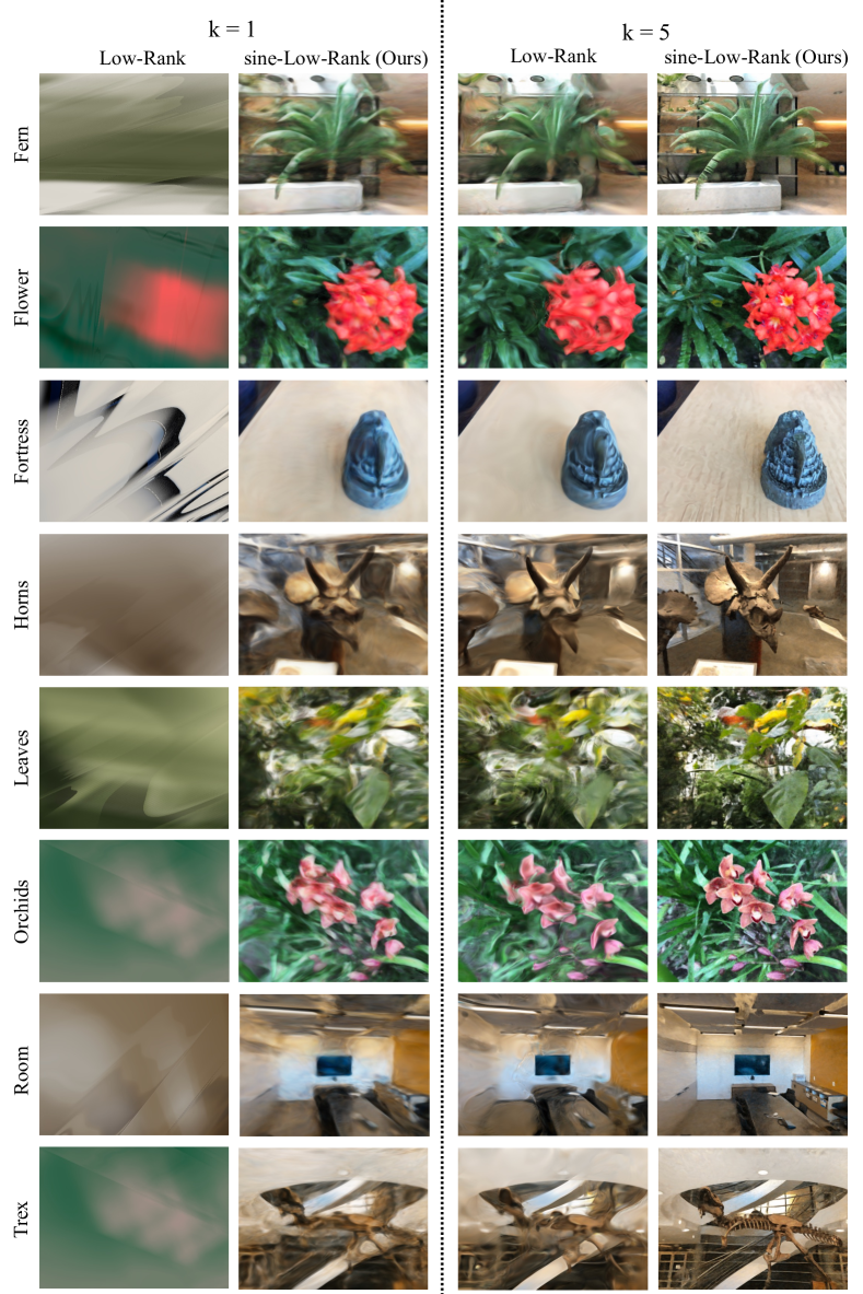
Figure 4: Qualitative NeRF results for the LLFF dataset [24, 25] using rank $k=1$ and $k=5$. Using a Low-Rank model leads to a complete loss of signal for $k=1$, however, applying sine is able to reconstruct details even at the extreme low-rank case. At $k=5$ the sine-Low-Rank model is noticeably sharper and clearer than using the Low-Rank.

Table 4: Quantitative results for NeRF evaluated on the LLFF dataset [24, 25]. Our sine-Low-Rank method outperforms the naive low-rank method across all levels $k$. For multiple instances (Fern, Flower, Leaves, Orchids, Room), the $k$=1 sine-Low-Rank model is able to outperform the $k$=5 model. We report the peak signal-to-noise ratio (PSNR) with the compression rate representing the percentage of parameters used in comparison to the parameter count of the Full-Rank NeRF model.

	PSNR$\uparrow$
	Fern	Flower	Fortress	Horn	Leaves	Orchids	Room	Trex	Average	Change	Compression Rate
Full-Rank	$26.38$	$27.54$	$30.93$	$28.20$	$21.79$	$21.33$	$30.96$	$27.68$	$26.85$	-	$100\%$
Low-Rankk=1	$15.03$	$14.60$	$14.74$	$13.66$	$12.89$	$12.50$	$15.04$	$13.54$	$14.00$	$\mathbf{5.77}$ ↑	1.3%
sine-Low-Rankk=1	20.77	20.14	24.13	19.00	15.92	16.25	25.53	16.42	19.77
Low-Rankk=5	$20.64$	$19.81$	$24.90$	$20.40$	$15.74$	$16.07$	$22.74$	$19.79$	$20.01$	$\mathbf{3.12}$ ↑	4.7%
sine-Low-Rankk=5	23.50	23.27	26.78	23.99	18.49	18.90	27.05	22.96	23.11
Low-Rankk=10	$22.83$	$22.18$	$25.96$	$22.76$	$17.36$	$18.12$	$26.12$	$21.69$	$22.12$	$\mathbf{2.27}$ ↑	8.7%
sine-Low-Rankk=10	24.56	24.61	28.01	25.39	19.62	20.02	28.70	24.21	24.39
Low-Rankk=30	$24.48$	$24.68$	$28.10$	$25.54$	$19.36$	$20.04$	$38.92$	$24.24$	$24.42$	$\mathbf{1.45}$ ↑	24.6%
sine-Low-Rankk=30	25.71	26.01	29.46	27.16	20.95	21.17	30.18	26.27	25.86
Low-Rankk=60	$25.26$	$26.16$	$29.50$	$26.74$	$20.39$	$20.85$	$30.00$	$25.81$	$25.59$	$\mathbf{0.74}$ ↑	48.6%
sine-Low-Rankk=60	26.09	26.70	29.75	27.78	21.56	21.37	30.54	27.16	26.36

Neural Radiance Field (NeRF) represents 3D scene signals by utilizing a set of 2D sparse images[25]. The 3D reconstruction is obtained by a forward pass $f_{\theta}(x,y,z,\theta,\phi)$, involving position ($x,y,z$) and viewing direction $(\theta,\phi)$. We evaluate our methods by training a NeRF model on the standard benchmarks LLFF dataset, which consists of 8 real-world scenes captured by hand-held cameras [24]. To evaluate our method on NeRF we substitute each fully dense layer with low-rank decomposition and use a range of rank levels ($k$).

Results. Tab. 4 demonstrates that employing low-rank matrices in NeRF learning reduces parameter count while significantly enhancing compression. However, performance dips with very low rank levels ($k$), where models capture minimal information. Our methods, nevertheless, substantially elevate performance. For instance, with $k=1$, our sine-Low-Rank approach yields an average PSNR of 19.77, outperforming the naive low-rank by 5.77 and achieving a compression rate of merely $1.3\%$. Even at a $48\%$ compression rate, it surpasses the basic low-rank model by 0.8 PSNR, narrowly trailing the baseline by just 0.45 PSNR, as shown in Figs. 4 and 5. Our rate-distortion analysis, applying Akima interpolation for Bjøntegaard Delta calculation, reveals a BD-Rate of $-64.72\%$ and BD-PSNR of 2.72dB, signifying marked improvements in compression efficiency[2, 16].

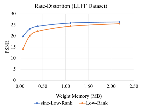
Figure 5: Rate-Distortion curve for NeRF results (average over the LLFF dataset). The sine-Low-Rank NeRF models show significant rate-distortion improvement relative to the naive low-rank NeRF. Evaluating the Bjøntegaard Delta between the models using Akima interpolation shows BD-Rate: -64.72% and BD-PSNR: 2.72dB, indicating substantial improvement in compression quality from using the sine-Low-Rank model.

Analysis. NeRF models, to a certain degree, tend to overfit entire 3D scenes, and a high training PSNR usually leads to a high testing PSNR. Employing structured weight matrices could result in a drop in performance due to the inherent constraints imposed by their structural design. Increasing the matrices’ rank enhances their memorization abilities significantly, especially when using a very low rank level $k$. Starting from a low frequency, there is a rapid and consistent increase in PSNR. Consequently, as we elevate the rank level $k$, our results gradually align with the baseline NeRFs, which serve as the upper bound.

4.4 3D shape modeling

For this experiment, we evaluate the binary occupancy task, which involves determining whether a given space or environment is occupied [23]. Following [28], we sampled over a 512 $\times$ 512 $\times$ 512 grid with each voxel within the volume assigned a 1, and voxels outside the volume assigned a 0. We evaluate intersection over union (IoU) for the occupancy volumes. We used a coordinate-based MLP that includes two hidden layers, each with a width of 256 neurons, and employed the Gaussian activation function. The full-rank model achieves an accuracy of 97 (IoU) and further details are presented in supplementary materials. Fig. 6 shows the 3D mesh representation of the Thai Statue, visualized using the low-rank method and the sine-Low-Rank method for $k=1,2,5$. Applying the sine function to the low-rank matrix resulted in a significant enhancement and more precise shape delineation.

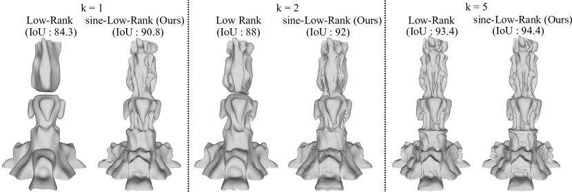
Figure 6: Binary occupancy field reconstruction on the Thai Statue instance from the Stanford Scanning Repository. Note that without a sine function, the Low-Rank model is unable reconstruct any finer details for the $k=1$ case; however, even at that level the sine-Low-Rank model is able to reconstruct fine structural details of the statue, including the trunks of the elephants. The $k=1$, $k=2$ and $k=5$ model utilizes only 2.1%, 2.9% and 5.2%, respectively, of the parameters of the full-rank model.

5 Limitations

Our exploration into sine-activated low-rank matrices illuminates their promising capabilities, yet it also has a limitation: notably, while these matrices can reach rank levels comparable to their full-rank counterparts upon the application of a sine function, their accuracy falls short. This highlights an ongoing challenge in finding the optimal balance between the need for sufficient parameterization to ensure high accuracy and the preferable rank of matrices. Overparameterization is widely recognized in the literature as vital for deep learning models to achieve strong generalization and optimization outcomes. However, our approach, despite increasing the rank, does not provide a clear pathway to achieving an efficient representation that can equal the accuracy of a full-rank model. Moving forward, developing strategies that not only enhance the rank but also clearly define the necessary degree of overparameterization will be crucial for creating cost-effective deep learning architectures, presenting an intriguing avenue for future research.

6 Conclusion

In this work, we developed a strategy that elevates the efficacy of general machine learning models, that employ feedforward layers, through parameter-efficient learning without additional parameter costs. Employing low-rank matrices reduces parameter cost, yet overly aggressive reductions, such as to rank=1, can detrimentally impact performance. Our method integrates a sine function within low-rank matrix decompositions to increase the rank of the decomposition leading to yielding an effective method to surmount their constrained representational capacity, thereby boosting model performance while maintaining the parameter cost. We gave a theoretical argument detailing why this method works and went on to validate the theory empirically on a variety of large-scale deep learning models over a broad set of applications. Furthermore, our findings reveal that learning with low-rank matrices contributes to mitigating overfitting, thereby facilitating the effective training of models even on limited datasets.

7 Acknowledgement

The authors thank Xueqian Li, Jianqiao Zheng, Shin-Fang Chng, and Daisy Bai for helpful discussion.

Appendix 0.A Theoretical Framework

In this section we give the proof of Prop. 1 and Thm. 3.1 from Sec. 3.2 of the paper.

We recall from Sec. 3.2 the following notation: For fixed fixed $\omega\,{>}\,0$, let $\sin(\omega\,{\cdot}\,\mathbf{A})$ denote the matrix obtained from a fixed $m{\times}n$ matrix $\mathbf{A}$ by applying the function $\sin(\omega\,{\cdot}\,\mathbf{x})$ component-wise to $\mathbf{A}$. Assuming $\mathbf{A}\,{\neq}\,0$ we define $A_{\min}^{0}$ as:

$$A_{\min}^{0}=\min_{i,js.t.A_{ij\neq 0}}|A_{ij}|.$$ (7)

Note that such a quantity is well defined precisely because $\mathbf{A}$ has a finite number of entries and all such entries cannot be zero from the assumption that $\mathbf{A}\,{\neq}\,0$.

Before we give the proof of Prop. 1, we will prove two lemmas.

Lemma 1

For a fixed $m{\times}n$ matrix $\mathbf{A}$. We have

$$||sin(\omega\mathbf{A})||^{2}_{F}\geq\omega^{2}(A_{\min}^{0})\text{ if }0<\omega<\frac{\pi}{3A_{\min}^{0}}$$ (8)

where $A_{\min}^{0}$ is defined as follows:

$$A_{\min}^{0}=\min_{i,js.t.A_{ij\neq 0}}|A_{ij}|$$ (9)

for $1\,{\leq}\,i\,{\leq}\,m$ and $1\,{\leq}\,j\,{\leq}\,n$.

Proof

Observer by definition of the Frobenius norm that

$$||sin(\omega\mathbf{A})||_{F}^{2}=\sum_{i=1}^{m}\sum_{j=1}^{n}sin(\omega\mathbf{A}_{ij})^{2}.$$ (10)

Now observe that if $\mathbf{A}_{ij}\,{=}\,0$ then the term $sin(\omega\mathbf{A}_{ij})^{2}\,{=}\,0$ and hence does not contribute to the above sum. Therefore, we find that

$$||sin(\omega\mathbf{A})||_{F}^{2}\geq sin(\omega A_{\min}^{0})^{2}.$$ (11)

The goal is to now find a lower bound on $sin(\omega A_{\min}^{0})^{2}$. In order to do this consider the function $f(\omega)\,{=}\,sin(\omega x)\,{-}\,\frac{\omega x}{2}$, where $x\,{\in}\,\mathbb{R}$ is fixed and positive.

Differentiating this function we have

$$f^{\prime}(\boldsymbol{\omega})=xcos(\boldsymbol{\omega}x)-\frac{x}{2}.$$ (12)

To find a critical point we solve the equation $f^{\prime}(\boldsymbol{\omega})\,{=}\,0$ to find

$$cos(\boldsymbol{\omega}x)=\frac{1}{2}.$$ (13)

Eq. 13 has the solution $\omega x\,{=}\,\frac{\pi}{3}$. In order to check what type of critical point $\boldsymbol{\omega}x\,{=}\,\frac{\pi}{3}$ we need to look at $f^{\prime\prime}(\boldsymbol{\omega})$

$$f^{\prime\prime}(\boldsymbol{\omega})=-x^{2}sin(\boldsymbol{\omega}x)<0$$ (14)

when $\omega\,{=}\,\frac{\pi}{3x}$ implying that the critical point $\omega\,{=}\,\frac{\pi}{3x}$ is a maximum point.

Observe that $f(0)\,{=}\,0$ it thus follows that $f(\boldsymbol{\omega})\,{\geq}\,0$ on the interval $[0,\frac{\pi}{3x}]$.

Applying this to the function $sin(\boldsymbol{\omega}A_{\min}^{0})$ we obtain that

$$sin(\boldsymbol{\omega}A_{\min}^{0})\geq\frac{\boldsymbol{\omega}A_{\min}^{0}}{2}\text{ if }0\leq\boldsymbol{\omega}\leq\frac{\pi}{3A_{\min}^{0}}.$$ (15)

Substituting the lower bound in Eq. 15 into Eq. 11, we obtain the proposition.

The next lemma establishes an upper bound on the operator norm of $sin(\omega A)$. We remind the reader that the operator norm of $A$

Lemma 2

Let $A$ be a fixed $m{\times}n$ matrix. Then

$$||sin(\omega\mathbf{A})||_{op}^{2}\leq||\sqrt{\omega}\sqrt{|\mathbf{A}|}||_{op}^{2}$$ (16)

where $\sqrt{|\mathbf{A}|}$ denotes the matrix obtained from $A$ by taking the absolute value and then square root component wise.

Proof

By definition we have

$$||sin(\omega\mathbf{A})||_{op}^{2}=\sup_{||x||_{2}=1}||sin(\omega\mathbf{A})x||_{2}^{2}$$ (17)

where $||\cdot||_{2}$ denotes the $2$-norm of a vector.

For any fixed unit vector $x$ we will show how to upper bound the quantity $||sin(\omega\mathbf{A})x||_{2}^{2}$. In order to do this we will use the fact that for $x\,{\geq}\,0$, we have the bound $sin(x)\,{\leq}\,\sqrt{|x|}$.

$$||sin(\omega\mathbf{A})x||_{2}^{2} =\sum_{i=1}^{m}\bigg{(}\sum_{j=1}^{n}sin(\omega A_{ij})x_{j}\bigg{)}^{2}$$ (18)

$$\leq\sum_{i=1}^{m}\bigg{(}\sum_{j=1}^{n}\sqrt{\omega}\sqrt{|\mathbf{A}_{ij}|}x_{j}\bigg{)}^{2}$$ (19)

$$=||(\sqrt{\omega})\bigg{(}\sqrt{|\mathbf{A}|}\bigg{)}x||^{2}_{2}.$$ (20)

It follows that

$$\sup_{||x||=1}||sin(\omega\mathbf{A})x||_{2}^{2}\leq\sup_{||x||=1}||\sqrt{\omega}\sqrt{|\mathbf{A}|}x||^{2}_{2}$$ (21)

which implies

$$||sin(\omega\mathbf{A})||_{op}^{2}\leq||\sqrt{\omega}\sqrt{|\mathbf{A}|}||^{2}_{op}.$$ (22)

We can now give the proof of Prop. 1 of the main paper. In order to do so we will need the definition of the stable rank of a matrix. Assume $\mathbf{A}$ is a non-zero $m{\times}n$ matrix. We define the stable rank of $\mathbf{A}$ by

$$SR(A):=\frac{||\mathbf{A}||_{F}^{2}}{||\mathbf{A}||_{op}^{2}}.$$ (23)

It is easy to see from the definition that the stable rank is continuous, unlike the rank, and is bounded above by the rank

$$SR(\mathbf{A})\leq Rank(\mathbf{A}).$$ (24)

Proof (of Prop. 3.1 from Sec. 3.2 of main paper)

Observe that from Eq. 24 it suffices to prove the lower bound on $SR(\mathbf{A})$. This is immediate from lemma 1 and lemma 2.

We can also give the proof of Thm. 1.

Proof (of Thm. 3.1 from Sec. 3.2 of main paper)

From the assumption of the Thm. 3.1, we have that $N\,{\gg}\,k$. Further, we are assuming that both $\mathbf{U}$ and $\mathbf{V}$ have entries sampled from $\mathcal{U}(-1/N,1/N)$. This means if we let $\mathbf{A}\,{=}\,\mathbf{U}\mathbf{V}^{T}$, then there exists a $C>0$ such that

$$A^{0}_{\min}=\frac{C}{N^{2}}.$$ (25)

Furthermore, observe that

$$||\sqrt{|\mathbf{A}|}||_{op}\leq||\sqrt{|\mathbf{A}|}||_{F}\leq||\mathbf{A}||_{F}$$ (26)

which implies

$$\omega\bigg{(}\frac{A^{0}_{\min}}{||\sqrt{|\mathbf{A}|}||_{op}}\bigg{)}^{2}\geq\omega\bigg{(}\frac{C}{N^{4}}\bigg{)}\bigg{(}\frac{N^{4}}{mn}\bigg{)}=\omega(\frac{C}{mn}).$$ (27)

Now observe that from Prop. 1 we have that

$$Rank(sin(\omega\mathbf{A}))\geq\omega\frac{A^{0}_{\min}}{||\sqrt{|\mathbf{A}|}||_{op}}$$ (28)

if $0\,{\leq}\,\omega\,{\leq}\,\frac{\pi}{3A^{0}_{\min}}$. We can rewrite this last condition to say that Eq. 28 holds if $0\,{\leq}\,\omega\,{\leq}\,\frac{\pi N^{2}}{3}$. In particular, by using Eq. 27 we find that there exists $\omega_{0}$ within the interval $0\,{\leq}\,\omega_{0}\,{\leq}\,\frac{\pi N^{2}}{3}$

$$Rank(sin(\omega_{0}\mathbf{A}))\,{\geq}\,\omega_{0}\frac{A^{0}_{\min}}{||\sqrt{|\mathbf{A}|}||_{op}}\,{\geq}\,k\,{\geq}\,Rank(\mathbf{A}).$$ (29)

This completes the proof.

Appendix 0.B Ablation study

In this section, we present additional results from ViT-Small, NeRF, and 3D shape modeling to demonstrate the superiority of our methods.

Table 5: This table illustrates the Top-1 Accuracy in pretraining the ViT-Small model with rank=1 on the CIFAR100 dataset using different frequencies, $\omega$, of sin($\omega\cdot$)

	PSNR
Low-Rankk=1	54.5
sine-Low-Rankk=1,ω=100	55.0
sine-Low-Rankk=1,ω=200	55.8
sine-Low-Rankk=1,ω=300	56.8
sine-Low-Rankk=1,ω=400	58.0
sine-Low-Rankk=1,ω=500	$\mathbf{58.1}$
sine-Low-Rankk=1,ω=600	57.6
sine-Low-Rankk=1,ω=700	57.5

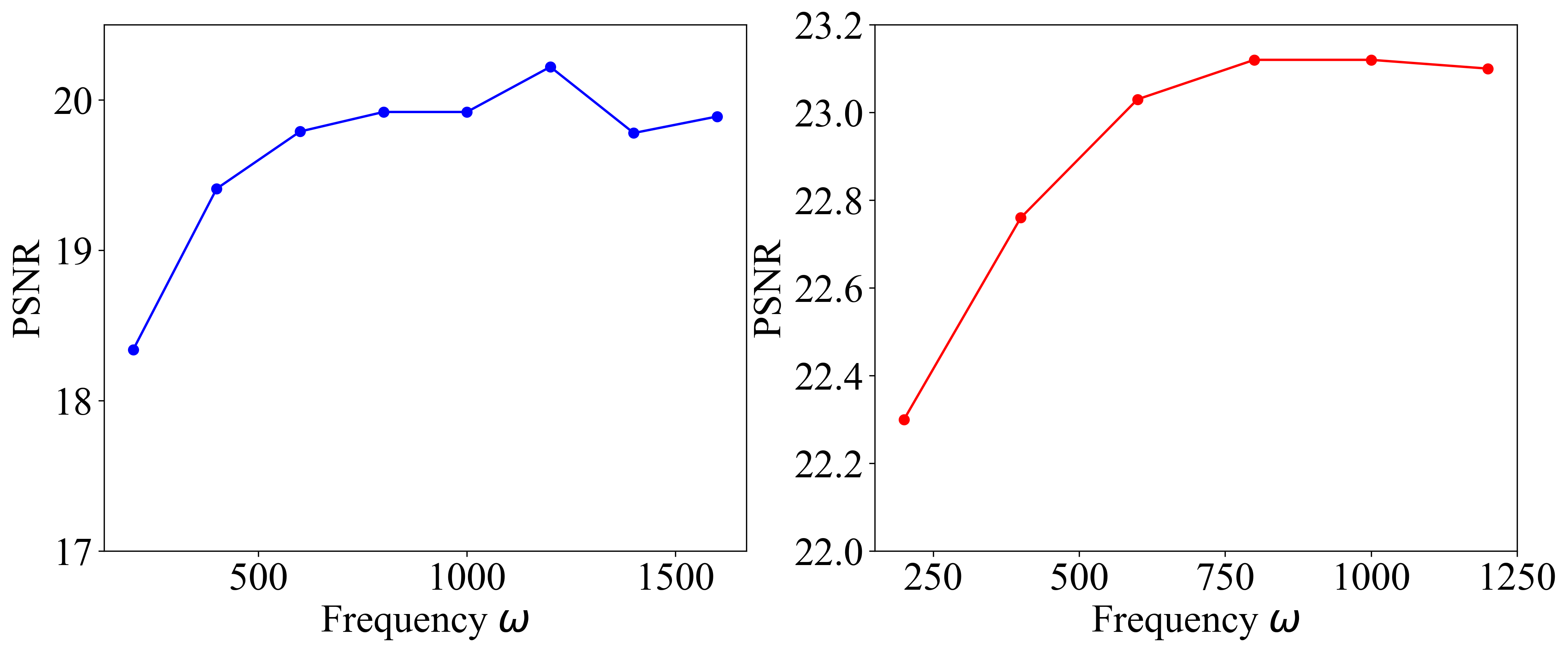
Figure 7: Ablation NeRF results for the LLFF dataset. These two figures show PSNR of NeRF using different frequencies when k=1 (on the left) and k=5 (on the right)

0.B.1 ViT-Small on CIFAR100

In Tab. 5, we examine the performance of our method on training the ViT-Small model from scratch on the CIFAR100 dataset using different frequencies, when rank=1.

Table 6: This table illustrates Intersection over Union (IoU) for 3D shape modeling across different rank levels ($k$). It also includes the compression rate, indicating the proportion of parameters utilized relative to the total parameter count of the baseline model, thereby detailing the parameter usage versus model performance at different levels of model complexity.

	Intersection	Compression
	over Union	Rate
Full-Rank	97.2	100%
Low-Rankk=1	84.3	2.1%
Sine-Low-Rankk=1	90.8
Low-Rankk=2	88.0	2.9%
Sine-Low-Rankk=2	92.0
Low-Rankk=5	93.4	5.2%
Sine-Low-Rankk=5	94.3
Low-Rankk=20	95.4	16.8%
Sine-Low-Rankk=20	95.4

Figure 8: Ablation binary occupancy results for Thai Statue. This figure shows IoU accuracy of 3D shape modeling using different frequencies, when k=1.

0.B.2 NeRF

In Fig. 7, we illustrate the impact of varying frequency on PSNR for cases where k=1 (shown on the left) and k=5 (shown on the right).

0.B.3 3D shape modelling

Tab. 6 reports the Itersection over Union (IoU) and Compression Rate of the binary occupancy task using different rank levels (k). Fig. 8 illustrates IoU using different frequencies when k=1.

References

- [1] Bentivogli, L., Clark, P., Dagan, I., Giampiccolo, D.: The fifth pascal recognizing textual entailment challenge. TAC 7(8), 1 (2009)
- [2] Bjøntegaard, G.: Calculation of average psnr differences between rd-curves. Tech. rep., VCEG-M33, Austin, TX, USA (April 2001)
- [3] Candès, E.J., Li, X., Ma, Y., Wright, J.: Robust principal component analysis? Journal of the ACM (JACM) 58(3), 1–37 (2011)
- [4] Cer, D., Diab, M., Agirre, E., Lopez-Gazpio, I., Specia, L.: SemEval-2017 task 1: Semantic textual similarity multilingual and crosslingual focused evaluation. In: Bethard, S., Carpuat, M., Apidianaki, M., Mohammad, S.M., Cer, D., Jurgens, D. (eds.) Proceedings of the 11th International Workshop on Semantic Evaluation (SemEval-2017). pp. 1–14. Association for Computational Linguistics, Vancouver, Canada (Aug 2017). https://doi.org/10.18653/v1/S17-2001, https://aclanthology.org/S17-2001
- [5] Chen, A., Xu, Z., Geiger, A., Yu, J., Su, H.: Tensorf: Tensorial radiance fields. In: Computer Vision – ECCV 2022: 17th European Conference, Tel Aviv, Israel, October 23–27, 2022, Proceedings, Part XXXII. p. 333–350. Springer-Verlag, Berlin, Heidelberg (2022). https://doi.org/10.1007/978-3-031-19824-3_20, https://doi.org/10.1007/978-3-031-19824-3_20
- [6] Dagan, I., Glickman, O., Magnini, B.: The PASCAL recognising textual entailment challenge. In: Machine learning challenges. evaluating predictive uncertainty, visual object classification, and recognising tectual entailment, pp. 177–190. Springer (2006)
- [7] Deng, J., Dong, W., Socher, R., Li, L.J., Li, K., Fei-Fei, L.: Imagenet: A large-scale hierarchical image database. In: 2009 IEEE Conference on Computer Vision and Pattern Recognition. pp. 248–255 (2009). https://doi.org/10.1109/CVPR.2009.5206848
- [8] Dettmers, T., Pagnoni, A., Holtzman, A., Zettlemoyer, L.: Qlora: Efficient finetuning of quantized llms. Advances in Neural Information Processing Systems 36 (2024)
- [9] Dolan, W.B., Brockett, C.: Automatically constructing a corpus of sentential paraphrases. In: Proceedings of the International Workshop on Paraphrasing (2005)
- [10] Dosovitskiy, A., Beyer, L., Kolesnikov, A., Weissenborn, D., Zhai, X., Unterthiner, T., Dehghani, M., Minderer, M., Heigold, G., Gelly, S., Uszkoreit, J., Houlsby, N.: An image is worth 16x16 words: Transformers for image recognition at scale. ICLR (2021)
- [11] Giampiccolo, D., Magnini, B., Dagan, I., Dolan, B.: The third PASCAL recognizing textual entailment challenge. In: Proceedings of the ACL-PASCAL workshop on textual entailment and paraphrasing. pp. 1–9. Association for Computational Linguistics (2007)
- [12] Glorot, X., Bengio, Y.: Understanding the difficulty of training deep feedforward neural networks. In: Proceedings of the thirteenth international conference on artificial intelligence and statistics. pp. 249–256. JMLR Workshop and Conference Proceedings (2010)
- [13] Haim, R.B., Dagan, I., Dolan, B., Ferro, L., Giampiccolo, D., Magnini, B., Szpektor, I.: The second pascal recognising textual entailment challenge. In: Proceedings of the Second PASCAL Challenges Workshop on Recognising Textual Entailment. vol. 7, pp. 785–794 (2006)
- [14] He, K., Chen, X., Xie, S., Li, Y., Dollár, P., Girshick, R.: Masked autoencoders are scalable vision learners. In: Proceedings of the IEEE/CVF conference on computer vision and pattern recognition. pp. 16000–16009 (2022)
- [15] He, K., Zhang, X., Ren, S., Sun, J.: Delving deep into rectifiers: Surpassing human-level performance on imagenet classification. In: 2015 IEEE International Conference on Computer Vision (ICCV). pp. 1026–1034 (2015). https://doi.org/10.1109/ICCV.2015.123
- [16] Herglotz, C., Kränzler, M., Mons, R., Kaup, A.: Beyond bjøntegaard: Limits of video compression performance comparisons. In: International Conference on Image Processing (ICIP) (2022). https://doi.org/10.1109/icip46576.2022.9897912
- [17] Hu, E.J., Shen, Y., Wallis, P., Allen-Zhu, Z., Li, Y., Wang, S., Wang, L., Chen, W.: LoRA: Low-rank adaptation of large language models. In: International Conference on Learning Representations (2022), https://openreview.net/forum?id=nZeVKeeFYf9
- [18] Jia, M., Tang, L., Chen, B.C., Cardie, C., Belongie, S., Hariharan, B., Lim, S.N.: Visual prompt tuning. In: European Conference on Computer Vision. pp. 709–727. Springer (2022)
- [19] Kopiczko, D.J., Blankevoort, T., Asano, Y.M.: Vera: Vector-based random matrix adaptation. In: International Conference on Learning Representations (2024)
- [20] Krizhevsky, A.: Learning multiple layers of features from tiny images. University of Toronto (05 2012)
- [21] Li, Y., Yu, Y., Liang, C., Karampatziakis, N., He, P., Chen, W., Zhao, T.: Loftq: LoRA-fine-tuning-aware quantization for large language models. In: The Twelfth International Conference on Learning Representations (2024), https://openreview.net/forum?id=LzPWWPAdY4
- [22] Menghani, G.: Efficient deep learning: A survey on making deep learning models smaller, faster, and better. ACM Comput. Surv. 55(12) (mar 2023). https://doi.org/10.1145/3578938, https://doi.org/10.1145/3578938
- [23] Mescheder, L., Oechsle, M., Niemeyer, M., Nowozin, S., Geiger, A.: Occupancy networks: Learning 3d reconstruction in function space. In: Proceedings IEEE Conf. on Computer Vision and Pattern Recognition (CVPR) (2019)
- [24] Mildenhall, B., Srinivasan, P.P., Ortiz-Cayon, R., Kalantari, N.K., Ramamoorthi, R., Ng, R., Kar, A.: Local light field fusion: Practical view synthesis with prescriptive sampling guidelines. ACM Transactions on Graphics (TOG) (2019)
- [25] Mildenhall, B., Srinivasan, P.P., Tancik, M., Barron, J.T., Ramamoorthi, R., Ng, R.: Nerf: Representing scenes as neural radiance fields for view synthesis. In: ECCV (2020)
- [26] Rajpurkar, P., Zhang, J., Lopyrev, K., Liang, P.: SQuAD: 100,000+ questions for machine comprehension of text. In: Proceedings of EMNLP. pp. 2383–2392. Association for Computational Linguistics (2016)
- [27] Reimers, N., Gurevych, I.: Sentence-bert: Sentence embeddings using siamese bert-networks. In: Proceedings of the 2019 Conference on Empirical Methods in Natural Language Processing. Association for Computational Linguistics (11 2019), http://arxiv.org/abs/1908.10084
- [28] Saragadam, V., LeJeune, D., Tan, J., Balakrishnan, G., Veeraraghavan, A., Baraniuk, R.G.: Wire: Wavelet implicit neural representations. In: Proceedings of the IEEE/CVF Conference on Computer Vision and Pattern Recognition (CVPR). pp. 18507–18516 (June 2023)
- [29] Schwarz, J.R., Tack, J., Teh, Y.W., Lee, J., Shin, J.: Modality-agnostic variational compression of implicit neural representations. In: Krause, A., Brunskill, E., Cho, K., Engelhardt, B., Sabato, S., Scarlett, J. (eds.) Proceedings of the 40th International Conference on Machine Learning. Proceedings of Machine Learning Research, vol. 202, pp. 30342–30364. PMLR (23–29 Jul 2023), https://proceedings.mlr.press/v202/schwarz23a.html
- [30] Sharma, P., Ash, J.T., Misra, D.: The truth is in there: Improving reasoning in language models with layer-selective rank reduction. arXiv preprint arXiv:2312.13558 (2023)
- [31] Shi, J., Guillemot, C.: Light field compression via compact neural scene representation. In: ICASSP 2023 - 2023 IEEE International Conference on Acoustics, Speech and Signal Processing (ICASSP). pp. 1–5 (2023). https://doi.org/10.1109/ICASSP49357.2023.10095668
- [32] Strang, G.: Linear Algebra and Learning from Data. Wellesley-Cambridge Press (2019)
- [33] Sun, C., Shrivastava, A., Singh, S., Gupta, A.: Revisiting unreasonable effectiveness of data in deep learning era. In: Proceedings of the IEEE International Conference on Computer Vision (ICCV) (Oct 2017)
- [34] Tang, J., Chen, X., Wang, J., Zeng, G.: Compressible-composable nerf via rank-residual decomposition. arXiv preprint arXiv:2205.14870 (2022)
- [35] Wang, A., Singh, A., Michael, J., Hill, F., Levy, O., Bowman, S.R.: Glue: A multi-task benchmark and analysis platform for natural language understanding. arXiv preprint arXiv:1804.07461 (2018)
- [36] Warstadt, A., Singh, A., Bowman, S.R.: Neural network acceptability judgments. arXiv preprint arXiv:1805.12471 (2018)
- [37] Williams, A., Nangia, N., Bowman, S.R.: A broad-coverage challenge corpus for sentence understanding through inference. In: Proceedings of NAACL-HLT (2018)
- [38] Xinwei, O., Zhangxin, C., Ce, Z., Yipeng, L.: Low rank optimization for efficient deep learning: Making a balance between compact architecture and fast training. Journal of Systems Engineering and Electronics PP, 1–23 (01 2023). https://doi.org/10.23919/JSEE.2023.000159
- [39] Xu, Z., Chen, Y., Vishniakov, K., Yin, Y., Shen, Z., Darrell, T., Liu, L., Liu, Z.: Initializing models with larger ones. In: International Conference on Learning Representations (ICLR) (2024)
- [40] Yu, X., Liu, T., Wang, X., Tao, D.: On compressing deep models by low rank and sparse decomposition. In: Proceedings of the IEEE conference on computer vision and pattern recognition. pp. 7370–7379 (2017)
- [41] Yuan, S., Zhao, H.: Slimmerf: Slimmable radiance fields (2023)
- [42] Zaken, E.B., Ravfogel, S., Goldberg, Y.: Bitfit: Simple parameter-efficient fine-tuning for transformer-based masked language-models. arXiv preprint arXiv:2106.10199 (2021)
- [43] Zhang, M., Chen, H., Shen, C., Yang, Z., Ou, L., Yu, X., Zhuang, B.: LoRAPrune: Pruning meets low-rank parameter-efficient fine-tuning (2024), https://openreview.net/forum?id=9KVT1e1qf7
- [44] Zheng, J., Li, X., Lucey, S.: Convolutional initialization for data-efficient vision transformers. arXiv preprint arXiv:2401.12511 (2024)