Regularized dynamical parametric approximation

Abstract

This paper studies the numerical approximation of evolution equations by nonlinear parametrizations $u(t)=\Phi(q(t))$ with time-dependent parameters $q(t)$, which are to be determined in the computation. The motivation comes from approximations in quantum dynamics by multiple Gaussians and approximations of various dynamical problems by tensor networks and neural networks. In all these cases, the parametrization is typically irregular: the derivative $\Phi^{\prime}(q)$ can have arbitrarily small singular values and may have varying rank. We derive approximation results for a regularized approach in the time-continuous case as well as in time-discretized cases. With a suitable choice of the regularization parameter and the time stepsize, the approach can be successfully applied in irregular situations, even though it runs counter to the basic principle in numerical analysis to avoid solving ill-posed subproblems when aiming for a stable algorithm. Numerical experiments with sums of Gaussians for approximating quantum dynamics and with neural networks for approximating the flow map of a system of ordinary differential equations illustrate and complement the theoretical results.

Keywords.  Time-dependent nonlinear parametric approximation, regularization, high-dimensional differential equation, Schrödinger equation, time integration, deep neural network, multi-Gaussian approximation.

1 Introduction

1.1 Nonlinear parametric approximation of evolution problems

We consider the numerical approximation of a possibly high-dimensional initial-value problem of ordinary or partial differential equations

$$\dot{y}=f(y),\qquad y(0)=y_{0}$$ (1)

via a nonlinear parametrization

$$y(t)\approx u(t)=\Phi(q(t)),\qquad 0\leq t\leq\overline{t},$$ (2)

with time-dependent parameters $q(t)$. Here, $\Phi$ is a smooth map from a parameter space into the solution space. We are interested in the situation of irregular parametrizations: the derivative matrix $\Phi^{\prime}(q)$ may have arbitrarily small singular values and possibly also varying rank. This is a typical situation of over-approximation that frequently arises in applications and causes severe numerical difficulties. Our motivation for studying such problems originated from the following areas, for which references are given and discussed in Subsection 1.3.

• Multi-Gaussian approximations in quantum dynamics: Here the parameters are the evolving complex width matrices, positions, momenta, and phases in a sum of complex Gaussians.

• Tensor network approximations in quantum dynamics: Here the parameters are the evolving connection tensors and bases.

• Deep neural network approximations of dynamical problems: Here the parameters are the evolving weight matrices and biases of the various layers of the neural network.

In all these cases, the derivative matrix $\Phi^{\prime}(q)$ typically has numerous very small singular values.

1.2 Regularized dynamical parametric approximation

In the numerical approach considered in this paper, we determine the time derivatives $\dot{q}(t)$ and $\dot{u}(t)=\Phi^{\prime}(q(t))\dot{q}(t)$ by solving the regularized linear least squares problem (we omit the argument $t$)

$$\|\dot{u}-f(u)\|^{2}+\varepsilon^{2}\|\dot{q}\|^{2}=\min!$$ (3)

with a possibly time-dependent regularization parameter $\varepsilon(t)>0$. This yields a differential equation for the parameters $q$, and then $u=\Phi(q)$. We refer to this approximation as a regularized dynamical parametric approximation. The resulting differential equation for $q$ is solved numerically by a standard time-stepping method, where each function evaluation solves a linear least squares problem (3).

This algorithmic approach is studied here even though the differential equation for the parameters $q$ is severely ill-conditioned for small $\varepsilon$. Errors in the initial value $q(0)$ can increase by a factor $e^{ct/\varepsilon}$ (with a constant $c>0$ independent of $\varepsilon$) to errors in $q(t)$ at times $t>0$. The approach thus appears to run counter to a basic principle of numerical analysis: to avoid solving ill-posed subproblems when aiming for a stable algorithm.

As a consequence of the ill-posedness in the parameters, also the error propagation in the solution approximation $u(t)=\Phi(q(t))$ is ill-behaved, but nevertheless the problem turns out to be what might be called well-posed up to the order of the defect size $O(\delta)$, where $\delta=\max_{0\leq t\leq\bar{t}}\delta(t)$ and $\delta(t)^{2}$ is the minimum value attained in (3) at time $t$. This beneficial behaviour is found both in the differential equation that results from (3) and in its numerical time discretization, and this makes the regularization (3) a viable computational approach. Its analysis adds new aspects to that of the underlying differential equation (1) and the time discretization.

One possibly obvious finding from our analysis is that good pointwise approximability of the solution $y(t)$ by parametrized functions is not sufficient. It is important that the time derivative $\dot{y}(t)$ can be well approximated in the tangent spaces at parametrized functions $u=\Phi(q)$ near $y(t)$. This suffices when $f$ is Lipschitz-continuous. In the case of a dominant term $Ay$ in $f(y)=Ay+g(y)$ with an unbounded operator $A$ that maps parametrized functions into their tangent space (a situation encountered for the Schrödinger equation), we need that $\dot{y}(t)-Ay(t)$ can be well approximated in the tangent space, and the regularized least-squares problem (3) should be slightly modified.

Remark 1 (Truncation vs. regularization)

As an alternative to regularizing the least-squares problem as in (3), small singular values of the matrix $A=\Phi^{\prime}(q)$ below a threshold $\varepsilon>0$ are set to zero, yielding a truncated matrix $A_{\varepsilon}$ with smallest nonzero singular value at least $\varepsilon$. Instead of (3), the time derivative $\dot{q}$ is then determined to be of minimal norm such that

$$\|A_{\varepsilon}(q)\dot{q}-f(\Phi(q))\|^{2}=\min!$$ (4)

Because of discontinuities in $A_{\varepsilon}(\cdot)$ when singular values cross the threshold, the resulting differential equation $\dot{q}=A_{\varepsilon}(q)^{+}f(\Phi(q))$ with the Moore–Penrose pseudo-inverse $A_{\varepsilon}^{+}$ has a discontinuous right-hand side and is problematic to analyse. After time discretization, however, this approach can be analysed by arguments that are entirely analogous to the regularized approach (3) and it is found to behave in a very similar way, since $A_{\varepsilon}^{+}$ behaves similarly to the matrix $(A^{\top}A+\varepsilon^{2}I)^{-1}A^{\top}$ that appears in the normal equations for (3). Both matrices have the same singular vectors and the singular values are $\sigma_{i}^{-1}$ if $\sigma_{i}\geq\varepsilon$ and zero else, and $(\sigma_{i}^{2}+\varepsilon^{2})^{-1}\sigma_{i}$, respectively, where $\sigma_{i}$ are the singular values of $A$.

1.3 Related work

In quantum dynamics, the non-regularized approach (3) with $\varepsilon=0$ is known as the Dirac–Frenkel time-dependent variational principle and has been widely used in computational chemistry and quantum physics over the past decades; see the books kramer1981 ; Lub08 for dynamic, geometric and approximation aspects and among countless papers see e.g. Joubert24 ; worth2004novel ; richings2015quantum with Gaussian wavepackets, meyer1990multi ; wang2003multilayer and shi2006classical ; haegeman2016unifying with tensor networks and carleo2017solving ; hartmann2019neural ; schmitt2020quantum with artificial neural networks. This approach usually leads to ill-conditioned least squares problems which cause numerical difficulties. Ad hoc regularization is often used in computations in such cases, but a systematic foundation and analysis appear to be missing in the literature. The regularization chosen in richings2015quantum corresponds precisely to (3) but is not further investigated there. The work KO2001 analyzes and proposes several regularization schemes in the context of Krylov-subspace projections of the original problem. This is of interest if one additionally wants to analyze the solution process of the arising linear systems, which we do not study here.

In recent years, an extensive amount of research has been invested in nonlinear approximations of differential equations, in particular in the context of neural networks. The majority of the literature relies on minimizing the residual in space-time, which yields a nonlinear optimization problem for the parameters globally in time. Prominent examples of such a strategy include the “deep Ritz method” BW18 as well as “weak generative adversarial networks” ZBYZ20 and both were successfully applied to a wide range of partial differential equations (see e.g. ZZKP19 ; BUMM21 ; BBGJJ21 ; KZBKKAA23 ). The nonlinear optimization process is, however, difficult to analyse and the existing theory consequently focuses on the expressivity properties of neural networks, i.e., what approximation is theoretically possible (see e.g. OPS20 ; MM23 ; KPRS2022 ). This of course excludes the much harder task of training the network and explaining the success of these methods remains evasive.

An alternative approach in the literature is to use Galerkin based methods to obtain differential equations for the parameters, see e.g. ZBYZ20 . The Dirac–Frenkel time-dependent variational principle has been used outside the realm of quantum dynamics in the context of deep neural networks, for example in DZ21 (referred to as “evolutional deep neural network”) and in BPV24 (referred to as “neural Galerkin schemes”).

1.4 Outline

After establishing notation and framework in Section 2, we derive a posteriori and a priori error bounds for the time-continuous regularized approach (3) in Section 3, where we also study the sensitivity of approximations to initial values.

In Section 4 we study the error behaviour of the time discretization by the explicit and implicit Euler methods, where we observe in particular the interplay between the time stepsize and the regularization parameter. In Section 5 the result is extended to Runge-Kutta discretizations, for which we prove an optimal-order error bound up to the defect size $\delta$. In Section 6 we propose an adaptive selection of the regularization parameter and the stepsize that is based on the previous error analysis.

In Section 7 we study the effect of enforcing conserved quantities, which are typically not preserved by the regularized parametric approach.

In Section 8 we study the regularization approach for the time-dependent Schrödinger equation as an important exemplary case of an evolutionary partial differential equation.

Finally, in Section 9 we present two numerical examples that illustrate the behaviour of the regularized parametric approximation: first by a neural network to approximate the flow map of a system of ordinary differential equations, and second by a linear combination of complex Gaussians to approximate quantum dynamics.

In an appendix we collect some useful results on regularized least-square problems.

2 Regularized dynamical parametric approximation

We start with the formulation of the framework. Let the state space ${\cal H}$ be a Hilbert space (finite- or infinite-dimensional) with the inner product $\langle\cdot,\cdot\rangle_{\cal H}$ and corresponding norm $\|\cdot\|_{\cal H}$ and let the parameter space ${\cal Q}$ be a finite-dimensional vector space equipped with the inner product $\langle\cdot,\cdot\rangle_{\cal Q}$ and corresponding norm $\|\cdot\|_{\cal Q}$. The parametrization map $\Phi:{\cal Q}\to{\cal H}$ is assumed to be twice continuously differentiable. It need not be one-to-one, not even locally. The derivative $\Phi^{\prime}(q)$ may have arbitrarily small singular values and a nontrivial nullspace of varying dimension.

The initial value in (1) is assumed to be in parametrized form: $y(0)=\Phi(q(0))$ for some $q(0)\in{\cal Q}$. We take $u(0)=y(0)=\Phi(q(0))$.

For $t\geq 0$, let $\varepsilon(t)>0$ be the regularization parameter. For $u(t)\in{\cal H}$ and $q(t)\in{\cal Q}$ with $u(t)=\Phi(q(t))$, the time derivatives $\dot{u}(t)=\Phi^{\prime}(q(t))\dot{q}(t)\in{\cal H}$ and $\dot{q}(t)\in{\cal Q}$ are determined by requiring that

$$\delta(t)^{2}:=\|\dot{u}(t)-f(u(t))\|_{\cal H}^{2}+\varepsilon(t)^{2}\|\dot{q}(t)\|_{\cal Q}^{2}\quad\text{is minimal.}$$ (5)

In this regularized linear least squares problem, $\dot{q}(t)$ is uniquely determined, which it would not necessarily be without the regularization.

The graph

$${\cal M}=\{(u,q)\,:\,u=\Phi(q)\}\subset{\cal H}\times{\cal Q}$$

need not be a manifold, but at $(u,q)\in{\cal M}$ it has the tangent space

$$T_{(u,q)}{\cal M}=\{(\dot{u},\dot{q})\,:\,\dot{u}=\Phi^{\prime}(q)\dot{q}\}\subset{\cal H}\times{\cal Q}.$$

Remark 2

With respect to the $\varepsilon$-weighted inner product on ${\cal H}\times{\cal Q}$ that is defined by $\langle\cdot,\cdot\rangle_{\cal H}+\varepsilon^{2}\langle\cdot,\cdot\rangle_{\cal Q}$, we consider the orthogonal projection onto $T_{(u,q)}{\cal M}$, denoted

$$P_{(u,q)}^{\varepsilon}:{\cal H}\times{\cal Q}\to T_{(u,q)}{\cal M}.$$

Then, (5) is equivalent to (omitting the argument $t$)

$$(\dot{u},\dot{q})=P_{(u,q)}^{\varepsilon}\bigl{(}f(u),0\bigr{)}.$$ (6)

While this reformulation is reminiscent of the useful interpretation of the Dirac–Frenkel time-dependent variational principle as a projection, see (Lub08, , Section II.1), the difficulty here is that $P_{(u,q)}^{\varepsilon}$ has no moderate Lipschitz constant with respect to $(u,q)$ under our assumptions, as is quantified in Proposition 4 below. The Lipschitz-continuity of the projection onto the tangent space was an essential condition in the proof of quasi-optimality of the approximation obtained from the Dirac–Frenkel time-dependent variational principle in (Lub08, , Section II.6). This is not available here, and so the question arises as to what alternative kind of error analysis can still be done.

3 Error bounds

In this section we assume that the vector field $f:{\cal H}\to{\cal H}$ in the differential equation (1) is a Lipschitz-continuous map, with the one-sided Lipschitz constant $\ell$ and the Lipschitz constant $L$ : for all $v,w\in{\cal H}$,

$${\mathrm{Re}\,}\langle v-w,f(v)-f(w)\rangle_{\cal H} \leq\ell\,\|v-w\|_{\cal H}^{2},$$ (7)

$$\|f(v)-f(w)\|_{\cal H} \leq L\,\|v-w\|_{\cal H}.$$

The real part is taken in the case of a complex-linear space ${\cal H}$.

3.1 A posteriori error bound

For the defect $d(t)$ of the approximation $u=\Phi(q)$ we have

$$\dot{u}(t)=f(u(t))+d(t)\qquad\text{with}\quad\|d(t)\|_{\cal H}\leq\delta(t)$$ (8)

for $\delta(t)$ of (5). There is the following error bound in terms of $\delta$.

Proposition 1

In the situation of Section 2 and with the one-sided Lipschitz condition (7), the error is bounded by

$$\|u(t)-y(t)\|_{\cal H}\leq\int_{0}^{t}e^{\ell(t-s)}\,\delta(s)\,ds.$$

Proof

The proof is standard and is included for the convenience of the reader. We subtract (1) from (8) and take the inner product with $u-y$ and its real part (if ${\cal H}$ is a complex space). On the left-hand side this yields, omitting the omnipresent argument $t$,

$${\mathrm{Re}\,}\langle u-y,\dot{u}-\dot{y}\rangle=\frac{1}{2}\frac{d}{dt}\|u-y\|^{2}=\|u-y\|\cdot\frac{d}{dt}\|u-y\|$$

and on the right-hand side

$${\mathrm{Re}\,}\langle u-y,f(u)-f(y)+d\rangle\leq\|u-y\|\bigl{(}\ell\,\|u-y\|+\delta\bigr{)}.$$

Dividing both sides by $\|u-y\|$ and using Gronwall’s inequality yields the result. ∎

While $\delta(t)$ can be monitored during the computation and is thus available a posteriori, we have not bounded it a priori from known or assumed approximability properties of the exact solution. This is done next.

3.2 A priori error bound

We will bound the defect size $\delta(t)$ by a quantity that measures the approximability of the solution derivative $\dot{y}(t)$ in the tangent spaces $T_{(u,q)}{\cal M}$ for all $u=\Phi(q)$ in a neighbourhood of $y(t)$. We fix a radius $\rho>0$ such that there exist parametrized functions $u=\Phi(q)$ with $\|u-y(t)\|_{\cal H}\leq\rho$, and define

$$\bar{\delta}_{\rho}(t)^{2}:=\sup_{q\in{\cal Q}:\|\Phi(q)-y(t)\|_{\cal H}\leq\rho}\ \min_{\dot{q}\in{\cal Q}}\Bigl{(}\|\Phi^{\prime}(q)\dot{q}-\dot{y}(t)\|^{2}+\varepsilon^{2}\|\dot{q}\|^{2}\Bigr{)}.$$ (9)

We can bound $\delta(t)$ of (5) in terms of $\bar{\delta}_{\rho}(t)$.

Lemma 1

Provided that $\|u(t)-y(t)\|\leq\rho$, we have

$$\ \delta(t)\leq\bar{\delta}_{\rho}(t)+\|f(u(t))-f(y(t))\|_{\cal H}.$$

Proof

We omit the argument $t$ in the following. We have $u=\Phi(q)$ and $\dot{u}=\Phi^{\prime}(q)\dot{q}$. Let $\dot{q}_{+}\in{\cal Q}$ be such that

$$\|\Phi^{\prime}(q)\dot{q}_{+}-\dot{y}\|_{\cal H}^{2}+\varepsilon^{2}\|\dot{q}_{+}\|_{\cal Q}^{2}\quad\text{is minimal.}$$

We obtain from (5), (9) and $\dot{y}=f(y)$

$$\delta^{2} =\|\Phi^{\prime}(q)\dot{q}-f(u)\|_{\cal H}^{2}+\varepsilon^{2}\|\dot{q}\|_{\cal Q}^{2}$$

$$\leq\|\Phi^{\prime}(q)\dot{q}_{+}-f(u)\|_{\cal H}^{2}+\varepsilon^{2}\|\dot{q}_{+}\|_{\cal Q}^{2}$$

$$\leq\Bigl{(}\|\Phi^{\prime}(q)\dot{q}_{+}-\dot{y}\|_{\cal H}+\|f(y)-f(u)\|_{\cal H}\Bigr{)}^{2}+\varepsilon^{2}\|\dot{q}_{+}\|_{\cal Q}^{2}$$

$$\leq{\bar{\delta}_{\rho}}^{\,2}+2\bar{\delta}_{\rho}\,\|f(y)-f(u)\|_{\cal H}+\|f(y)-f(u)\|_{\cal H}^{2}$$

$$=\Bigl{(}\bar{\delta}_{\rho}+\|f(y)-f(u)\|_{\cal H}\Bigr{)}^{2}.$$

Taking square roots yields the result. ∎

We construct a reference approximation $u_{*}(t)=\Phi(q_{*}(t))$ with $q_{*}(t)\in{\cal Q}$ from the exact solution such that its derivative is a regularized best approximation in the tangent space at $(u_{*}(t),q_{*}(t))$ to the solution derivative $\dot{y}(t)$. The derivatives $\dot{u}_{*}(t)=\Phi^{\prime}(q_{*}(t))\dot{q}_{*}(t)$ and $\dot{q}_{*}(t)$ are determined such that

$$\delta_{*}(t)^{2}:=\|\dot{u}_{*}(t)-\dot{y}(t)\|_{\cal H}^{2}+\varepsilon^{2}\|\dot{q}_{*}(t)\|_{\cal Q}^{2}\quad\text{is minimal}.$$ (10)

Here we have the immediate error bound

$$\|u_{*}(t)-y(t)\|_{\cal H}\leq\int_{0}^{t}\|\dot{u}_{*}(s)-\dot{y}(s)\|_{\cal H}\,ds\leq\int_{0}^{t}\delta_{*}(s)\,ds\leq\int_{0}^{t}\bar{\delta}_{\rho}(s)\,ds$$ (11)

as long as this bound does not exceed $\rho$. The following result bounds the error of the numerical approximation $u(t)$ by a multiple of the bound in (11).

Proposition 2

In the situation of Section 2 and under the Lipschitz condition (7), the error is bounded by

$$\|u(t)-y(t)\|_{\cal H}\leq e^{(\ell+L)t}\int_{0}^{t}\bar{\delta}_{\rho}(s)\,ds$$

as long as this does not exceed $\rho$.

Proof

The bound follows from Lemma 1 inserted into the proof of Proposition 1 and using the Lipschitz condition on $f$ and the Gronwall lemma. ∎

3.3 Sensitivity to initial values

Given two initial values $y_{0},\widetilde{y}_{0}\in{\cal H}$, the difference of the correponding solutions $y(t)$ and $\widetilde{y}(t)$ of the differential equation (1) are bounded, under the one-sided Lipschitz condition (7), by

$$\|y(t)-\widetilde{y}(t)\|_{\cal H}\leq e^{\ell t}\,\|y_{0}-\widetilde{y}_{0}\|_{\cal H},\qquad t\geq 0;$$

see e.g. (HW, , IV.12). There is no analogous result for the regularized approximations $u(t)=\Phi(q(t))$ and $\widetilde{u}(t)=\Phi(\widetilde{q}(t))$ with initial values $u_{0}=\Phi(q_{0})$ and $\widetilde{u}_{0}=\Phi(\widetilde{q}_{0})$, not even with the Lipschitz constant $L$ instead of $\ell$. We only obtain the following bound.

Proposition 3

Under the one-sided Lipschitz condition (7) we have

$$\|u(t)-\widetilde{u}(t)\|_{\cal H}\leq e^{\ell t}\,\|u_{0}-\widetilde{u}_{0}\|_{\cal H}+\int_{0}^{t}e^{\ell(t-s)}\bigl{(}\delta(s)+\widetilde{\delta}(s)\bigr{)}ds,\quad\ t\geq 0,$$ (12)

with the defect size $\delta(t)$ of (5) and analogously $\widetilde{\delta}(t)$ corresponding to $\widetilde{u}(t)$.

Proof

This bound is obtained by the argument of Proposition 1 and estimating the difference of the defects $d(t)=\dot{u}(t)-f(u(t))$ of (8) and analogously $\widetilde{d}(t)$ in a rough way by $\|d(t)-\widetilde{d}(t)\|_{\cal H}\leq\delta(t)+\widetilde{\delta}(t)$. ∎

Note that the right-hand side of (12) does not tend to zero as $u_{0}-\widetilde{u}_{0}\to 0$. The difference of the defects is bounded in this rough way because there does not seem to be a better way that does not introduce negative powers of $\varepsilon$ into the bound. The difficulty becomes apparent in the following bound for $\dot{u}(t)-\dot{\widetilde{u}}(t)$, where the second term on the right-hand side is a multiple of $\|q(t)-\widetilde{q}(t)\|_{\cal Q}$, which cannot be avoided and cannot be estimated by an $\varepsilon$-independent multiple of $\|u(t)-\widetilde{u}(t)\|_{\cal H}$, as we would like.

Proposition 4

As a function of $q$, we denote by $\dot{q}(q)$ the solution of the regularized least squares problem

$$\delta(q)^{2}=\|\Phi^{\prime}(q)\dot{q}(q)-f(\Phi(q))\|_{\cal H}^{2}+\varepsilon^{2}\|\dot{q}(q)\|_{\cal Q}^{2}\quad\text{is minimal}.$$ (13)

Then, for all $q,\widetilde{q}\in{\cal Q}$ and associated $u=\Phi(q)$, $\widetilde{u}=\Phi(\widetilde{q})$ and $\dot{u}=\Phi^{\prime}(q)\dot{q}(q)$, $\dot{\widetilde{u}}=\Phi^{\prime}(\widetilde{q})\dot{q}(\widetilde{q})$,

$$\|\dot{u}-\dot{\widetilde{u}}\|_{\cal H} \leq L\|u-\widetilde{u}\|_{\cal H}+\tfrac{5}{2}\beta\,\frac{\bar{\delta}}{\varepsilon}\,\|q-\widetilde{q}\|_{\cal Q},$$

$$\|\varepsilon\dot{q}(q)-\varepsilon\dot{q}(\widetilde{q})\|_{\cal Q} \leq L\|u-\widetilde{u}\|_{\cal H}+\tfrac{5}{2}\beta\,\frac{\bar{\delta}}{\varepsilon}\,\|q-\widetilde{q}\|_{\cal Q},$$

$$and\qquad|\delta(q)-\delta(\widetilde{q})| \leq 3L\|u-\widetilde{u}\|_{\cal H}+5\beta\frac{\bar{\delta}}{\varepsilon}\,\|q-\widetilde{q}\|_{\cal Q},$$

where $\beta$ is an upper bound on second order derivatives of $\Phi$ and $\bar{\delta}$ an upper bound on $\delta$ on the line segment between $q$ and $\widetilde{q}$, and $L$ is the Lipschitz constant of $f$ in (7).

Proof

We use the adjoint $\Phi^{\prime}(q)^{*}\in L({\cal H},{\cal Q})$ of the linear map $\Phi^{\prime}(q)\in L({\cal Q},{\cal H})$ and the normal equations $M_{\varepsilon}(q)\dot{q}(q)=\Phi^{\prime}(q)^{*}f(\Phi(q))$ with Gramian matrix $M_{\varepsilon}(q)=\Phi^{\prime}(q)^{*}\Phi^{\prime}(q)+\varepsilon^{2}I_{\cal Q}$. We denote

$$\Phi^{\prime}(q)\dot{q}(q) =\Phi^{\prime}(q)M_{\varepsilon}(q)^{-1}\Phi^{\prime}(q)^{*}f(\Phi(q))$$

$$=:P_{\varepsilon}(q)f(\Phi(q)).$$

By Lemma 8, we have $\|P_{\varepsilon}(q)\|_{L({\cal H})}\leq 1$ and therefore

$$\|P_{\varepsilon}({\widetilde{q}})(f(\Phi(q))-f(\Phi({\widetilde{q}})))\|_{\cal H}\leq L\|\Phi(q)-\Phi({\widetilde{q}})\|_{\cal H}.$$ (14)

As for the sensitivity of $P_{\varepsilon}(q)$ with respect to $q$, we consider the regularized least squares problem with fixed right hand side $b\in{\cal H}$ and its normal equation

$$M_{\varepsilon}(q)\dot{q}_{b}(q)=\Phi^{\prime}(q)^{*}b.$$

We differentiate

$$\partial_{q}M_{\varepsilon}(q)\dot{q}_{b}(q)+M_{\varepsilon}(q)\partial_{q}\dot{q}_{b}(q)=\partial_{q}\Phi^{\prime}(q)^{*}b$$

and obtain

$$\Phi^{\prime}(q)\partial_{q}\dot{q}_{b}(q)=\Phi^{\prime}(q)M_{\varepsilon}(q)^{-1}\left(\partial_{q}\Phi^{\prime}(q)^{*}b-\partial_{q}M_{\varepsilon}(q)\dot{q}_{b}(q)\right)$$

$$=\Phi^{\prime}(q)M_{\varepsilon}(q)^{-1}\left(\partial_{q}\Phi^{\prime}(q)^{*}\left(b-\Phi^{\prime}(q)\dot{q}_{b}(q)\right)-\Phi^{\prime}(q)^{*}\partial_{q}\Phi^{\prime}(q)\dot{q}_{b}(q)\right).$$

By Lemma 8, we have $\|\Phi^{\prime}(q)M_{\varepsilon}(q)^{-1}\|_{L({\cal Q},{\cal H})}\leq\frac{1}{2\varepsilon}$ and consequently

$$\|\Phi^{\prime}(q)\partial_{q}\dot{q}_{b}(q)\|_{\cal H} \leq\frac{\beta}{2\varepsilon}\|b-\Phi^{\prime}(q)\dot{q}_{\beta}(q)\|_{\cal H}+\beta\|\dot{q}_{b}(q)\|_{\cal Q}\leq\frac{3\beta}{2\varepsilon}\,\delta_{b}(q)$$

with

$$\delta_{b}(q)^{2}=\|\Phi^{\prime}(q)\dot{q}_{b}(q)-b\|_{\cal H}^{2}+\varepsilon^{2}\|\dot{q}_{b}(q)\|_{\cal Q}^{2}.$$

This implies, for

$$\partial_{q}(P_{\varepsilon}(q)b)=\partial_{q}(\Phi^{\prime}(q)\dot{q}_{b}(q))=\partial_{q}\Phi^{\prime}(q)\dot{q}_{b}(q)+\Phi^{\prime}(q)\partial_{q}\dot{q}_{b}(q),$$

the bound

$$\|\partial_{q}(P_{\varepsilon}(q)b)\|_{{\cal H}}\leq\frac{5\beta}{2\varepsilon}\,\delta_{b}(q).$$

Using this bound for the right-hand side $b=f(\Phi(q))$ and combining it with the Lipschitz estimate (14), we obtain

$$\|\Phi^{\prime}(q)\dot{q}(q)-\Phi^{\prime}({\widetilde{q}})\dot{q}({\widetilde{q}})\|_{\cal H}$$

$$\leq\|(P_{\varepsilon}(q)-P_{\varepsilon}({\widetilde{q}}))f(\Phi(q))\|_{\cal H}+\|P_{\varepsilon}({\widetilde{q}})(f(\Phi(q))-f(\Phi({\widetilde{q}})))\|_{\cal H}$$

$$\leq\frac{5\beta\bar{\delta}}{2\varepsilon}\|q-{\widetilde{q}}\|_{\cal Q}+L\|\Phi(q)-\Phi({\widetilde{q}})\|_{\cal H},$$

which is the first of the stated bounds. The second one follows in the same way. Finally, with $u=\Phi(q)$ and $\dot{u}=\Phi^{\prime}(q)\dot{q}$ and analogously $\widetilde{u}$ and $\dot{\widetilde{u}}$ we have by the Cauchy–Schwarz inequality and (13)

$$|\delta(q)^{2}-\delta(\widetilde{q})^{2}|=\big{|}\bigl{\langle}(\dot{u}-f(u))+(\dot{\widetilde{u}}-f(\widetilde{u})),(\dot{u}-\dot{\widetilde{u}})-(f(u)-f(\widetilde{u}))\bigr{\rangle}_{\cal H}$$

$$\qquad\qquad\qquad\qquad+\varepsilon^{2}\bigl{\langle}\dot{q}+\dot{\widetilde{q}},\dot{q}-\dot{\widetilde{q}}\bigr{\rangle}_{\cal Q}\big{|}$$

$$\leq\bigl{(}\delta(q)+\delta(\widetilde{q})\bigr{)}\,\bigl{(}\|\dot{u}-\dot{\widetilde{u}}\|_{\cal H}+\|f(u)-f(\widetilde{u})\|_{\cal H}\bigr{)}+\bigl{(}\delta(q)+\delta(\widetilde{q})\bigr{)}\,\varepsilon\|\dot{q}-\dot{\widetilde{q}}\|_{\cal Q},$$

which yields

$$|\delta(q)-\delta(\widetilde{q})|\leq\|\dot{u}-\dot{\widetilde{u}}\|_{\cal H}+L\|u-\widetilde{u}\|_{\cal H}+\varepsilon\|\dot{q}-\dot{\widetilde{q}}\|_{\cal Q},$$

and the stated bound follows from the first two bounds. ∎

Remark 3

As far as the inverse powers with respect to $\varepsilon$ are concerned, the previous estimates are sharp, as the following one-dimensional example with $\cal H={\cal Q}={\mathbb{R}}$, $\Phi(q)=\frac{1}{2}q^{2}$, and $f(u)=1$ illustrates. In this case we have

$$\dot{q}(q)=\frac{q}{q^{2}+\varepsilon^{2}},\quad d(q)=\Phi^{\prime}(q)\dot{q}(q)-f(u)=-\frac{\varepsilon^{2}}{q^{2}+\varepsilon^{2}}$$

and

$$\partial_{q}\dot{q}(q)=-\frac{q^{2}}{q^{2}+\varepsilon^{2}}+\frac{\varepsilon^{2}}{(q^{2}+\varepsilon^{2})^{2}}=-\frac{d(q)}{q^{2}+\varepsilon^{2}}-\frac{q^{2}}{q^{2}+\varepsilon^{2}}.$$

Moreover,

$$|\dot{u}-\dot{\widetilde{u}}| =\left|\frac{q}{q^{2}+\varepsilon^{2}}d(\widetilde{q})+\frac{\widetilde{q}}{\widetilde{q}^{2}+\varepsilon^{2}}d(q)\right|\left|q-\widetilde{q}\right|$$

$$=|\delta(q)-\delta(\widetilde{q})|$$

which implies

$$|\dot{u}-\dot{\widetilde{u}}|=|\delta(q)-\delta(\widetilde{q})|\leq\frac{\bar{\delta}}{\varepsilon}|q-\widetilde{q}|$$

$$|\varepsilon\dot{q}(q)-\varepsilon\dot{q}(\widetilde{q})|\leq\left(\varepsilon+\frac{\bar{\delta}}{\varepsilon}\right)|q-\widetilde{q}|.$$

These tight estimates exhibit the factor $\bar{\delta}/\varepsilon$ in the same way as the general bounds of Proposition 4.

Remark 4

Using Proposition 4 and Gronwall’s lemma, we obtain the bound

$$\|u(t)-\widetilde{u}(t)\|_{\cal H}+\varepsilon\|q(t)-\widetilde{q}(t)\|_{\cal Q}\leq e^{\omega t}\left(\|u_{0}-\widetilde{u}_{0}\|_{\cal H}+\varepsilon\|q_{0}-\widetilde{q}_{0}\|_{\cal Q}\right)$$

with the exponent $\omega=\max\bigl{(}\beta\bar{\delta}/\varepsilon^{2},L\bigr{)}$. For nonlinear parametrizations (where $\beta\neq 0$), which is our main interest in this paper, this is not a useful estimate for small $\varepsilon$. For linear parametrizations ($\beta=0$), however, we even obtain

$$\|u(t)-\widetilde{u}(t)\|_{\cal H}\leq e^{Lt}\|u_{0}-\widetilde{u}_{0}\|_{\cal H}$$

without any dependence on $\|q_{0}-\widetilde{q}_{0}\|_{\cal Q}$. Hence, with respect to error propagation, linear and nonlinear near-singular parametrizations behave very differently.

4 Time discretization by the regularized Euler method

We study time-stepping methods in the framework of Sections 2 and 3, first based on the Euler method and in the next section on general Runge–Kutta methods. The unusual feature is that the differential equation for the parameters $q$, which is the equation that is actually discretized, is ill-behaved, but nevertheless we find better behaviour of $u=\Phi(q)$. We only assume that the vector field $f$ in the original differential equation (1) for $y$ is sufficiently differentiable, and that the parametrization map $\Phi$ has bounded second derivatives (but a regular parametrization is not assumed). These properties will be used to derive error bounds for the discrete approximations $u_{n}=\Phi(q_{n})$ at $t_{n}=t_{0}+nh$, for stepsizes $h>0$ that need to be suitably restricted in terms of the defect in the regularized least squares problem and the regularization parameter. No error bounds are derived for the parameters $q_{n}$.

4.1 The regularized explicit Euler method

A step of the explicit Euler method applied to the differential equation for the parameters $q$, starting from $q_{n}$ at time $t_{n}$ with the regularization parameter $\varepsilon_{n}$, reads

$$q_{n+1}=q_{n}+h\dot{q}_{n},\qquad u_{n+1}=\Phi(q_{n+1}),$$ (15)

where $\dot{q}_{n}$ is the solution of the regularized linear least squares problem

$$\delta_{n}^{2}:=\|\Phi^{\prime}(q_{n})\dot{q}_{n}-f(u_{n})\|_{\cal H}^{2}+\varepsilon_{n}^{2}\|\dot{q}_{n}\|_{\cal Q}^{2}\quad\text{is minimal.}$$ (16)

4.2 Local error bound

We first consider the local error, that is the error after one step $u_{1}-y(t_{1})$, where $y(t)$ is the solution of (1) starting from $y(t_{0})=u_{0}=\Phi(q_{0})$.

Lemma 2

Under the stepsize restriction

$$h\delta_{0}\leq c\,\varepsilon_{0}^{2},$$ (17)

the local error of the regularized Euler method starting from $y(t_{0})=u_{0}$ is bounded by

$$\|u_{1}-y(t_{1})\|_{\cal H}\leq c_{1}h\delta_{0}+c_{2}h^{2}$$ (18)

with $c_{1}=1+c\beta$, where $\beta$ is a bound of the second derivative of $\Phi$ in a neighbourhood of $q_{0}$, and $c_{2}=\frac{1}{2}\max_{t_{0}\leq t\leq t_{1}}\|\ddot{y}(t)\|_{\cal H}$.

Proof

We have by Taylor expansion

$$y(t_{1})-y(t_{0}) =h\dot{y}(t_{0})+\int_{t_{0}}^{t_{1}}(t_{1}-t)\,\ddot{y}(t)\,dt$$

$$=hf(u_{0})+O(h^{2})$$

and we have

$$u_{1}-u_{0} =\Phi(q_{1})-\Phi(q_{0})$$

$$=\Phi^{\prime}(q_{0})(q_{1}\!-\!q_{0})+\!\!\int_{0}^{1}\!(1\!-\!\theta)\Phi^{\prime\prime}(q_{0}\!+\!\theta(q_{1}\!-\!q_{0}))[q_{1}\!-\!q_{0},q_{1}\!-\!q_{0}]\,d\theta$$

$$=\Phi^{\prime}(q_{0})h\dot{q}_{0}+O(\|h\dot{q}_{0}\|_{\cal Q}^{2})$$

$$=hf(u_{0})+O(h\delta_{0})+O\biggl{(}\Bigl{(}\frac{h\delta_{0}}{\varepsilon_{0}}\Bigr{)}^{2}\biggr{)},$$

where the last line results from the definition of $\delta_{0}$, which is an upper bound of both $\|\Phi^{\prime}(q_{0})\dot{q}_{0}-f(u_{0})\|_{\cal H}$ and $\varepsilon_{0}\|\dot{q}_{0}\|_{\cal Q}$. This implies $\|h\dot{q}_{0}\|_{\cal Q}\leq h\delta_{0}/\varepsilon_{0}$. Under the stepsize restriction $h\delta_{0}\leq c\varepsilon_{0}^{2}$, the last term is also $O(h\delta_{0})$. Subtracting the two formulas and tracing the constants in the $O(\cdot)$ terms yields the stated result. ∎

Remark 5

The result of Lemma 2 holds without any fixed bound on $\dot{q}_{0}$. If, however, $\|\dot{q}_{0}\|_{\cal Q}\leq\gamma$ with a moderate constant $\gamma$, which is satisfied if $\delta_{0}\leq\gamma\varepsilon_{0}$, then the above proof shows that the error bound (18) is satisfied with $c_{1}=1$ and $c_{2}=\frac{1}{2}\max_{t_{0}\leq t\leq t_{1}}\|\ddot{y}(t)\|_{\cal H}+\beta\gamma^{2}$ with the same $\beta$ as in the lemma. This clearly indicates that while the stepsize restriction (17) is sufficient for the stated error bound, it is not always necessary.

Remark 6

A local error estimate of a similar structure, without any restriction on the step size $h$ or the defect $\delta_{0}$, is readily available by keeping an additional a posteriori error term. Comparing the explicit Euler approximation $y_{1}=y_{0}+hf(y_{0})$ as an intermediate term with $u_{1}=\Phi(q_{1})$ yields

$$\|u_{1}-y(t_{1})\|_{\cal H}\leq\|u_{1}-y_{1}\|_{\cal H}+\|y_{1}-y(t_{1})\|_{\cal H}$$

$$\leq\|u_{1}-y_{0}-h\Phi^{\prime}(q_{0})\dot{q}_{0}\|_{\cal H}+h\|\Phi^{\prime}(q_{0})\dot{q}_{0}-f(u_{0})\|_{\cal H}+\|y_{1}-y(t_{1})\|_{\cal H}$$

$$\leq\|u_{1}-y_{0}-h\Phi^{\prime}(q_{0})\dot{q}_{0}\|_{\cal H}+h\delta_{0}+O(h^{2}).$$ (19)

The first term in the last line is computable with the quantities derived during the time integration of the scheme and comes at the cost of evaluating an additional $\mathcal{H}$-norm. Under the step size restriction of Lemma 2, or in the case of Remark 5, the term is of the optimal order $O(h\delta_{0}+h^{2})$.

4.3 Global error bound (using stable error propagation by the exact flow)

Using the standard argument of Lady Windermere’s fan with error propagation by the exact flow, see the book by Hairer, Nørsett & Wanner (HNW, , II.3), we obtain the following global error bound from Lemma 2 and condition (7).

Proposition 5

Under condition (7) and the stepsize restriction

$$h\delta_{n}\leq c\,\varepsilon_{n}^{2},\qquad 0\leq n\leq N,$$

the error of the regularized Euler method (15)–(16) with initial value $y_{0}=u_{0}=\Phi(q_{0})$ is bounded, for $t_{n}=nh\leq t_{N}\leq\bar{t}$, by

$$\|u_{n}-y(t_{n})\|_{\cal H}=O(\delta+h)\quad\text{with}\quad\delta=\max_{n}\delta_{n},$$

or more precisely (compare with Proposition 1),

$$\|u_{n}-y(t_{n})\|_{\cal H}\leq h\sum_{j=0}^{n-1}e^{\ell(t_{n-1}-t_{j})}\,\bigl{(}c_{1}\delta_{j}+c_{2}h),$$

where $c_{1}=1+c\beta$ with $\beta$ a bound of the second derivative of $\Phi$ in a neighbourhood of the solution, and $c_{2}$ is a bound of $f^{\prime}f$ in a neighbourhood of the solution $y(t)$, i.e. a bound of second derivatives of solutions $\widetilde{y}$ of the differential equation $\dot{\widetilde{y}}=f(\widetilde{y})$ with initial values in a neighbourhood of the solution trajectory $\{y(t):0\leq t\leq\bar{t}\}$.

4.4 Error propagation by the numerical method

The Euler method applied to (1) is stable in the sense that the numerical results $y_{1}$ and $\widetilde{y}_{1}$ obtained from starting values $y_{0}$ and $\widetilde{y}_{0}$, respectively, differ by

$$\|y_{1}-\widetilde{y}_{1}\|_{\cal H}\leq(1+hL)\|y_{0}-\widetilde{y}_{0}\|_{\cal H},$$

where $L$ is again the Lipschitz constant of $f$. For the regularized Euler method we only obtain, similarly to the proof of Lemma 2, a discrete analogue of (12):

$$\|u_{1}-\widetilde{u}_{1}\|_{\cal H}\leq(1+hL)\|u_{0}-\widetilde{u}_{0}\|_{\cal H}+h\delta_{0}+h\widetilde{\delta}_{0}.$$ (20)

This is not good enough to be used in Lady Windermere’s fan with error propagation by the numerical method, which is the most common way to prove error bounds for numerical methods for nonstiff differential equations; see HNW .

4.5 A priori error bound for the regularized explicit Euler method

The bound in Proposition 5 is partly a priori (in its dependence on $\ell$, $c_{1}$ and $c_{2}$) and partly a posteriori (in its dependence on the defect sizes $\delta_{j}$). In terms of the method-independent defect sizes $\bar{\delta}_{\rho}(t)$ $\rho$-near to the exact solution as defined in (9), we have the following discrete analogue of Proposition 2.

Proposition 6

In the situation of Proposition 5 we have the a priori error bound, for $0\leq t_{n}=nh\leq\bar{t}$,

$$\|u_{n}-y(t_{n})\|_{\cal H}\leq C_{1}h\sum_{j=1}^{n}\bar{\delta}_{\rho}(t_{j})+C_{2}h,$$

where $C_{1}$ and $C_{2}$ depend on $L\bar{t}$ but are independent of $h$ and $\varepsilon$. This bound is valid as long as the right-hand side does not exceed $\rho$.

Proof

We still have the bound of Lemma 1,

$$\delta_{n}\leq\bar{\delta}_{\rho}(t_{n})+\|f(u_{n})-f(y(t_{n}))\|_{\cal H}.$$

Inserting this bound in the local error bound of Proposition 5 and using the Lipschitz condition on $f$ yields

$$\|u_{n}-y(t_{n})\|_{\cal H}\leq c_{1}h\sum_{j=1}^{n}\bar{\delta}_{\rho}(t_{j})+c_{1}h\sum_{j=1}^{n}L\,\|u_{j}-y(t_{j})\|_{\cal H}+c_{2}h,$$

and the discrete Gronwall inequality yields the result. ∎

4.6 Regularized implicit Euler method

A step of the implicit Euler method, starting from $q_{n}$ at time $t_{n}$ reads

$$q_{n+1}=q_{n}+h\dot{q}_{n+1},\qquad u_{n+1}=\Phi(q_{n+1}),$$

where $\dot{q}_{n+1}$ is the solution of the regularized linear least squares problem

$$\delta_{n+1}^{2}=\|\Phi^{\prime}(q_{n+1})\dot{q}_{n+1}-f(u_{n+1})\|_{\cal H}^{2}+\varepsilon_{n+1}^{2}\|\dot{q}_{n+1}\|_{\cal Q}^{2}\quad\text{is minimal.}$$

The defining equation for $q_{n+1}$ is a fixed point equation $q_{n+1}=\varphi_{n}(q_{n+1})$ for the function

$$\varphi_{n}(q):=q_{n}+h\ \mathrm{argmin}_{\dot{q}\in{\cal Q}}\left(\|\Phi^{\prime}(q)\dot{q}-f(\Phi(q))\|_{\cal H}^{2}+\varepsilon_{n+1}^{2}\|\dot{q}\|_{\cal Q}^{2}\right).$$

This is a contraction for $h$ sufficiently small due to the bound of Proposition 4, which implies

$$\|\varphi_{n}(q)-\varphi_{n}(\widetilde{q})\|_{\cal Q}\leq h\left(\frac{\beta_{2}\bar{\delta}}{\varepsilon_{n+1}^{2}}+\frac{\beta_{1}L}{\varepsilon_{n+1}}\right)\|q-\widetilde{q}\|_{\cal Q}$$

for $\bar{\delta}>0$ an upper bound on the residual size in a neighbourhood of $q,\widetilde{q}$. The constants $\beta_{1},\beta_{2}>0$ depend on first order and second order derivatives of $\Phi$, respectively. Hence, with a step-size restriction of the form

$$h\left(\frac{\beta_{2}\bar{\delta}}{\varepsilon_{n+1}^{2}}+\frac{\beta_{1}L}{\varepsilon_{n+1}}\right)<1,$$

where $\bar{\delta}>0$ is an upper bound on the residual size in the vicinity of the numerical solution, the fixed point iteration is contractive and thus converging.

The local error satisfies

$$\|u_{1}-y(t_{1})\|_{\cal H}\leq\beta h^{2}\|\dot{q}_{1}\|^{2}_{\cal H}+h\delta_{1}+c_{2}h^{2},$$

as is seen by repeating the proof of Lemma 2 with obvious adaptations. This leads to global error bounds as in Propositions 5 and 6.

5 Regularized explicit Runge–Kutta methods

A step of an explicit Runge–Kutta method of order $p$ with coefficients $a_{ij}$ and $b_{j}$ applied to the differential equation for the parameters $q$ reads as follows. Starting from $q_{n}$ at time $t_{n}$ with the regularization parameter $\varepsilon_{n}$, we first compute consecutively the internal stages (for $i=1,\dots,s$)

$$q_{n,i}=q_{n}+h\sum_{j=1}^{i-1}a_{ij}\dot{q}_{n,j},\qquad u_{n,i}=\Phi(q_{n,i}),$$ (21)

and $\dot{q}_{n,i}$ as the solution of the regularized linear least squares problem

$$\delta_{n,i}^{2}:=\|\Phi^{\prime}(q_{n,i})\dot{q}_{n,i}-f(u_{n,i})\|_{\cal H}^{2}+\varepsilon_{n}^{2}\|\dot{q}_{n,i}\|_{\cal Q}^{2}\quad\text{is minimal.}$$ (22)

Finally, the new value is computed as

$$q_{n+1}=q_{n}+h\sum_{j=1}^{s}b_{j}\dot{q}_{n,j},\qquad u_{n+1}=\Phi(q_{n+1}).$$ (23)

We first bound the local error.

Lemma 3

Let $\delta_{0}=\max_{i}\delta_{0,i}$. Under the stepsize restriction

$$h\delta_{0}\leq c\,\varepsilon_{0}^{2},$$ (24)

the local error of the regularized $p$-th order Runge–Kutta method starting from $y(t_{0})=u_{0}=\Phi(q_{0})$ is bounded by

$$\|u_{1}-y(t_{1})\|_{\cal H}\leq c_{1}h\delta_{0}+c_{2}h^{p+1},$$ (25)

where $c_{1}$ is a constant times $1+c\beta$ with the bound $\beta$ of the second derivative of $\Phi$ in a neighbourhood of $q_{0}$, and $c_{2}h^{p+1}$ is the bound for the local error of the $p$-th order Runge–Kutta method applied to (1).

Proof

We note that (22) implies $\|\varepsilon_{0}\dot{q}_{0,j}\|_{\cal Q}\leq\delta_{0}$ and hence $\|h\dot{q}_{0,j}\|_{\cal Q}\leq h\delta_{0}/\varepsilon_{0}$. Moreover, (22) also implies $\|\Phi^{\prime}(q_{0,j})\dot{q}_{0,j}-f(u_{0,j})\|_{\cal H}\leq\delta_{0}$. This yields

$$u_{0,i}-u_{0}=\Phi(q_{0,i})-\Phi(q_{0})=\Phi^{\prime}(q_{0})h\sum_{j=1}^{i-1}a_{ij}\dot{q}_{0,j}+O\biggl{(}\Bigl{(}\frac{h\delta_{0}}{\varepsilon_{0}}\Bigr{)}^{2}\biggr{)}$$

$$=h\sum_{j=1}^{i-1}a_{ij}\Phi^{\prime}(q_{0,j})\dot{q}_{0,j}-\sum_{j=1}^{i-1}a_{ij}\bigl{(}\Phi^{\prime}(q_{0,j})-\Phi^{\prime}(q_{0})\bigr{)}h\dot{q}_{0,j}+O\biggl{(}\Bigl{(}\frac{h\delta_{0}}{\varepsilon_{0}}\Bigr{)}^{2}\biggr{)}$$

$$=h\sum_{j=1}^{i-1}a_{ij}f(u_{0,j})+O(h\delta_{0})+O\biggl{(}\Bigl{(}\frac{h\delta_{0}}{\varepsilon_{0}}\Bigr{)}^{2}\biggr{)}+O\biggl{(}\Bigl{(}\frac{h\delta_{0}}{\varepsilon_{0}}\Bigr{)}^{2}\biggr{)}$$

and in the same way

$$u_{1}-u_{0}=h\sum_{j=1}^{s}b_{j}f(u_{0,j})+O(h\delta_{0})+O\biggl{(}\Bigl{(}\frac{h\delta_{0}}{\varepsilon_{0}}\Bigr{)}^{2}\biggr{)}.$$

Apart from the $O(\cdot)$ terms, these formulae are those that define the result $y_{1}$ of one step of the Runge–Kutta method applied to (1). So we obtain, using also the Lipschitz continuity of $f$,

$$u_{1}-y_{1}=O(h\delta_{0})+O\biggl{(}\Bigl{(}\frac{h\delta_{0}}{\varepsilon_{0}}\Bigr{)}^{2}\biggr{)}.$$

Since the method is of order $p$ and $f$ is sufficiently differentiable, we have

$$y_{1}-y(t_{1})=O(h^{p+1}).$$

Noting that under the stepsize restriction (24) we have $({h\delta_{0}}/{\varepsilon_{0}})^{2}\leq ch\delta_{0}$, the error bound (25) follows. ∎

As before, using the local error bound in Lady Windermere’s fan with error propagation by the exact solutions, we obtain the following global error bound for the $p$-th order Runge method. We formulate the result for variable stepsizes $h_{n}$, so that $t_{n+1}=t_{n}+h_{n}$ and $t_{N}=\bar{t}$.

Proposition 7

Under condition (7) and the stepsize restriction

$$h_{n}\delta_{n,i}\leq c\,\varepsilon_{n}^{2},\qquad 0\leq n\leq N,\ \ i=1,\dots,s,$$

the error of the regularized $p$-th order Runge–Kutta method (21)–(23) with initial value $y_{0}=u_{0}=\Phi(q_{0})$ is bounded, for $t_{n}\leq\bar{t}$, by

$$\|u_{n}-y(t_{n})\|_{\cal H}=O(\delta+h^{p})$$

with $\delta=\max_{n,i}\delta_{n,i}$ and $h=\max_{n}h_{n}$. The constants symbolized by the O-notation are independent of $\,\delta$ and the regularization parameters $\varepsilon_{n}$ (under the given stepsize restriction), and of the stepsize sequence $(h_{k})$ and $n$ with $t_{n}\leq\bar{t}$.

6 Choice of the regularization parameter and the stepsize

The algorithm below chooses the regularization parameter $\varepsilon_{n}$ in the $n$th time step as large as possible such that the defect $\delta_{n}$ is within a given factor of the defect attained for tiny $\varepsilon$ or within a prescribed tolerance. The stepsize $h_{n}$ is chosen such that the critical quadratic error terms are of size $h_{n}\delta_{n}$.

For arbitrary $\varepsilon>0$, in the $n$th time step we let $\dot{q}_{n}(\varepsilon)$ be the solution of the regularized linear lest squares problem with regularization parameter $\varepsilon$ such that

$$\delta_{n}(\varepsilon)^{2}:=\|\Phi^{\prime}(q_{n})\dot{q}_{n}(\varepsilon)-f(u_{n})\|_{\cal H}^{2}+\varepsilon^{2}\|\dot{q}_{n}(\varepsilon)\|_{\cal Q}^{2}\quad\text{is minimal.}$$

Let $\varepsilon_{n}^{0}$ and $h_{n}^{0}$ be initializations of the regularization parameter and the stepsize, respectively. These might be the values from the previous time step. Let $\varepsilon_{\star}$ be a tiny reference parameter such that $\delta_{n}(\varepsilon_{\star})$ can still be computed reliably (just so). Let $\delta_{\min}>0$ be a given threshold.

6.1 Choice of the regularization parameter $\varepsilon_{n}$

Compute $\delta_{n}(\varepsilon_{\star})$ and set $\delta_{n}^{\rm tol}=\max(17\,\delta_{n}(\varepsilon_{\star}),\delta_{\min})$ as the target defect size. We aim at having $\delta_{n}(\varepsilon_{n})\approx\delta_{n}^{\rm tol}$. We use 1 or 2 Newton iterations for the equation $\delta_{n}(\varepsilon_{n})^{2}-(\delta_{n}^{\rm tol})^{2}=0$ (except in the very first step where a good starting value is not available and more iterations might be needed). In view of Lemma 7, which shows that this is a monotonically increasing concave smooth function with the derivative $d\delta_{n}^{2}/d\varepsilon^{2}=\|\dot{q}_{n}(\varepsilon)\|^{2}_{\cal Q}$, we have the Newton iteration

$$\left(\varepsilon_{n}^{k+1}\right)^{2}=\left(\varepsilon_{n}^{k}\right)^{2}-\frac{\delta_{n}(\varepsilon_{n}^{k})^{2}-\left(\delta_{n}^{\text{tol}}\right)^{2}}{\|\dot{q}_{n}(\varepsilon_{n}^{k})\|_{\cal Q}^{2}}.$$

Alternatively, we can proceed in a Levenberg–Marquardt style, cf. more2006levenberg :
Initialize $\varepsilon_{n}=\varepsilon_{n}^{0}$.
If $\delta_{n}(\varepsilon_{n})\leq\delta_{n}^{\rm tol}$
     then while $\delta_{n}(3\varepsilon_{n})\leq\delta_{n}^{\rm tol}$ set $\varepsilon_{n}:=3\varepsilon_{n}$
     else while $\delta_{n}(\varepsilon_{n})>\delta_{n}^{\rm tol}$ set $\varepsilon_{n}:=\varepsilon_{n}/3$.

In the following we set $\dot{q}_{n}=\dot{q}_{n}(\varepsilon_{n})$ and $\delta_{n}=\delta_{n}(\varepsilon_{n})$.

6.2 Choice of the stepsize $h_{n}$

The stepsize $h_{n}$ is chosen such that $\|\Phi^{\prime\prime}(q_{n})[h_{n}\dot{q}_{n},h_{n}\dot{q}_{n}]\|_{\cal H}\approx h_{n}\delta_{n}$. This is satisfied for the choice

$$h_{n}=\frac{h_{n}^{0}\delta_{n}}{\|(\Phi^{\prime}(q_{n}+h_{n}^{0}\dot{q}_{n})-\Phi^{\prime}(q_{n}))\dot{q}_{n}\|_{\cal H}}.$$

6.3 Regularized Runge–Kutta step with $\varepsilon_{n}$ and $h_{n}$

We compute $q_{n+1}$ and $u_{n+1}=\Phi(q_{n+1})$ by a regularized Runge–Kutta step (see Section 5) with the proposed regularization parameter $\varepsilon_{n}$ and the proposed stepsize $h_{n}$. We can use an embedded pair of Runge–Kutta methods that gives a local error estimate that should not substantially exceed $h_{n}\delta_{n}$ (else the step is rejected and repeated with a reduced stepsize).

7 Conserved quantities

7.1 Conserved quantities and regularized dynamical approximation

Let $g=(g_{1},\dots,g_{m})^{\top}:{\cal H}\to{\mathbb{R}}^{m}$ be an $m$-vector of real-valued functions that are conserved along the flow of the differential equation (1):

$$g(y(t))=g(y(0))\qquad\text{for all $t$}$$

for every choice of initial value $y(0)\in{\cal H}$. Differentiating this equation w.r.t. $t$, this is seen to be equivalent to

$$G(y(t))\dot{y}(t)=0,$$

where $G=g^{\prime}=\partial g/\partial y$, and hence to

$$G(y)f(y)=0\qquad\text{for all $y$}.$$

However, $g$ is no longer a conserved quantity for the regularized dynamical approximation (5), not even for linear $g$. We use the notation

$$A=\Phi^{\prime},\quad M_{\varepsilon}=A^{\top}\!A+\varepsilon^{2}I,\quad P_{\varepsilon}=AM_{\varepsilon}^{-1}\!A^{\top}$$

where we omitted the argument $q$ for all appearing matrices. For the regularized least squares problem (5) we have the normal equations (now omitting the argument $t$)

$$M_{\varepsilon}(q)\dot{q}=A(q)^{\top}f(\Phi(q))$$ (26)

and for $u=\Phi(q)$, the time derivative $\dot{u}=\Phi^{\prime}(q)\dot{q}$ becomes

$$\dot{u}=P_{\varepsilon}(q)f(u)=f(u)+d\quad\text{ with }\quad d=-(I-P_{\varepsilon}(q))f(u),$$ (27)

where the defect $d$ is bounded by $\|d\|_{\cal H}\leq\delta$ in view of (5). As $G(u)f(u)=0$, we obtain

$$\frac{d}{dt}\,g(u)=G(u)\dot{u}=G(u)d,$$

which in general is different from zero, so that $g(u(t))$ is not conserved. We note, however, the bound

$$|g(u(t))-g(u(0))|\leq K\int_{0}^{t}\delta(t)\,dt,$$

where $K$ is an upper bound of the norm of $G(u)$ along the trajectory $u(\cdot)$.

7.2 Enforcing conservation

We can enforce conservation of $g$ along the approximation $u(t)=\Phi(q(t))$ by adding the condition $G(u(t))\dot{u}(t)=0$ as a constraint, i.e. (omitting the argument $t$)

$$G(\Phi(q))A(q)\dot{q}=0,$$

and we minimize in (5) under this constraint. With the notation

$$C(q):=G(\Phi(q))A(q)=g^{\prime}(u)\Phi^{\prime}(q),$$

we obtain instead of (26) the constrained system with a Lagrange multiplier $\lambda(t)\in{\mathbb{R}}^{m}$,

$$M_{\varepsilon}(q) \dot{q}+C(q)^{\top}\lambda=A(q)^{\top}f(\Phi(q))$$ (28)

$$C(q) \dot{q}\hskip 45.5244pt=0.$$

Inserting $\dot{q}$ from the first equation into the second equation, we find $\lambda$ from the equation (omitting the argument $q$ or $u$ of the matrices)

$$CM_{\varepsilon}^{-1}C^{\top}\lambda=CM_{\varepsilon}^{-1}A^{\top}f(u)$$

or equivalently, since $C=GA$ and $P_{\varepsilon}=AM_{\varepsilon}^{-1}A^{\top}$ imply $CM_{\varepsilon}^{-1}C^{\top}=GP_{\varepsilon}G^{\top}$ and $CM_{\varepsilon}^{-1}A^{\top}=GP_{\varepsilon}$, and since $(P_{\varepsilon}-I)f(u)=d$ and $G(u)f(u)=0$, we find

$$\bigl{(}G(u)P_{\varepsilon}(q)G(u)^{\top}\bigr{)}\lambda=G(u)d.$$ (29)

The symmetric positive semi-definite matrix $P_{\varepsilon}=AM_{\varepsilon}^{-1}A^{\top}$ has the eigenvalues $\lambda_{i}=\sigma_{i}^{2}/(\sigma_{i}^{2}+\varepsilon^{2})$ and 0, where $\sigma_{i}$ are the singular values of $A$. Eigenvalues are very small if they correspond to very small singular values $\sigma_{i}\ll\varepsilon$ of $A$, but are larger than $\tfrac{1}{2}$ for $\sigma_{i}\geq\varepsilon$. To understand under which condition the symmetric positive semi-definite matrix $GP_{\varepsilon}G^{\top}$ has a moderately bounded inverse, let $\Lambda$ be the diagonal matrix of eigenvalues of $P_{\varepsilon}$ and $U$ the orthogonal matrix of eigenvectors, and for $\theta>0$ let $U_{\theta}$ be the matrix composed of those eigenvectors of $P_{\varepsilon}$ that correspond to the eigenvalues $\lambda_{i}\geq\theta$. If the smallest singular value of $GU_{\theta}$ equals $\rho>0$, then

$$\|(GP_{\varepsilon}G^{\top})^{-1}\|_{2}\leq\frac{1}{\theta\rho^{2}},$$ (30)

because $v^{\top}GU\Lambda(GU)^{\top}v\geq v^{\top}GU_{\theta}\Lambda_{\theta}(GU_{\theta})^{\top}v\geq\theta\|(GU_{\theta})^{\top}v\|_{2}^{2}\geq\theta\rho^{2}\|v\|_{2}^{2}$ for all $v\in{\mathbb{R}}^{m}$. Here, $\Lambda_{\theta}$ is the diagonal matrix of those eigenvalues of $P_{\varepsilon}$ that are larger than $\theta$. We remark that in the case of just one conserved quantity ($m=1$), the inverse of $GP_{\varepsilon}G^{\top}\in{\mathbb{R}}$ is moderately bounded if $\nabla g$ is not near-orthogonal to all those singular vectors of $A$ that correspond to singular values $\sigma_{i}\geq\varepsilon$. This appears to be a very mild requirement.

Inserting $\lambda$ from (29) into the first equation of (28) and using the definition of the defect $d$ yields $\dot{u}=A\dot{q}$ as

$$\dot{u}+P_{\varepsilon}G^{\top}(GP_{\varepsilon}G^{\top})^{-1}Gd=f(u)+d.$$

With the projection onto the null-space of $G(u)$ for $u=\Phi(q)$ that is given by

$$\Pi(q)=I-P_{\varepsilon}(q)G(u)^{\top}(G(u)P_{\varepsilon}(q)G(u)^{\top})^{-1}G(u),$$

we thus obtain for $u(t)=\Phi(q(t))$, instead of (27), the differential equation with the projected defect,

$$\dot{u}=f(u)+\Pi(q)d.$$ (31)

7.3 Constrained regularized Euler method

We now ensure the condition $g(u_{n+1})=g(u_{n})$ by adding it as a constraint to the regularized least squares problem (16). A step of the constrained regularized Euler method, starting from $q_{n}$ at time $t_{n}$ with the regularization parameter $\varepsilon_{n}$, reads

$$q_{n+1}=q_{n}+h\dot{q}_{n},\qquad u_{n+1}=\Phi(q_{n+1}),$$ (32)

where $\dot{q}_{n}$ is the solution of the constrained regularized linear least squares problem

$$\widehat{\delta}_{n}^{\,2}:=\|\Phi^{\prime}(q_{n})\dot{q}_{n}-f(u_{n})\|_{\cal H}^{2}+\varepsilon_{n}^{2}\|\dot{q}_{n}\|_{\cal Q}^{2}\quad\text{is minimal}$$ (33)

$$\text{subject to }\ g(u_{n+1})=g(u_{n}).$$

Note that while $\delta_{n}$ of (16) depends only on $q_{n}$, the defect size $\widehat{\delta}_{n}\geq\delta_{n}$ depends also on the stepsize $h$. With the notation of the previous subsections, a step of the unconstrained regularized Euler method of Section 4 reads (with $\varepsilon=\varepsilon_{n}$)

$$M_{\varepsilon}(q_{n})\dot{q}_{n}=A(q_{n})^{\top}f(u_{n})$$

together with $\widetilde{q}_{n+1}=q_{n}+h\dot{q}_{n}$ and $\widetilde{u}_{n+1}=\Phi(q_{n+1})$. The minimality condition for the constrained problem (33) now determines (a different) $\dot{q}_{n}$ together with the Lagrange multiplier $\lambda_{n+1}$ from the nonlinear system of equations

$$M_{\varepsilon}(q_{n})\dot{q}_{n}+C(q_{n})^{\top}\lambda_{n+1}=A(q_{n})^{\top}f(u_{n})$$ (34)

$$g\bigl{(}\Phi(q_{n}+h\dot{q}_{n})\bigr{)}=g(u_{n}).$$

We then set $q_{n+1}=q_{n}+h\dot{q}_{n}$ and $u_{n+1}=\Phi(q_{n+1})$. Inserting $\dot{q}_{n}$ from the first equation into the second equation, we get a nonlinear equation for $\lambda_{n+1}$: with $\widetilde{q}_{n+1}=q_{n}+hM_{\varepsilon}(q_{n})^{-1}A(q_{n})^{\top}f(u_{n})$ (which is the result of the unconstrained Euler method) we have

$$g\bigl{(}\Phi(\widetilde{q}_{n+1}-hM_{\varepsilon}(q_{n})^{-1}C(q_{n})^{\top}\lambda_{n+1})\bigr{)}-g(u_{n})=0.$$

A modified Newton method applied to this equation determines the $(k+1)$st iterate $\lambda_{n+1}^{(k+1)}=\lambda_{n+1}^{(k)}+\Delta\lambda_{n+1}^{(k)}$ by solving the linear system

$$-hC(q_{n})M_{\varepsilon}(q_{n})^{-1}C(q_{n})^{\top}\Delta\lambda_{n+1}^{(k)}$$ (35)

$$\qquad\qquad=-g\bigl{(}\Phi(\widetilde{q}_{n+1}-hM_{\varepsilon}(q_{n})^{-1}C(q_{n})^{\top}\lambda_{n+1}^{(k)})\bigr{)}+g(u_{n}).$$

The starting value is chosen as $\lambda_{n+1}^{(0)}=0$. The matrix $CM_{\varepsilon}^{-1}C^{\top}=GP_{\varepsilon}G^{\top}$ is the same as in (29). It is assumed to be invertible, see the bound (30) of the inverse.

Lemma 4

If the matrix $G(u_{n})P_{\varepsilon}(q_{n})G(u_{n})^{\top}$ has a moderately bounded inverse, then the modified Newton iteration (35) with starting value ${\lambda_{n+1}^{(0)}=0}$ converges under the stepsize restriction

$$h(\delta_{n}+h)\leq c\varepsilon$$

with a sufficiently small $c$ that is independent of $h$, $\varepsilon$ and $\delta$. Moreover,

$$\lambda_{n+1}=O(\delta_{n}+h).$$

Proof

The modified Newton iteration is a fixed-point iteration for the map (omitting the argument $u_{n}$ of $G$ and $q_{n}$ of $A,M_{\varepsilon},P_{\varepsilon}$ and letting $z=h\lambda$)

$$\varphi(z)=z-(GP_{\varepsilon}G^{\top})^{-1}\Bigl{(}g\bigl{(}\Phi(\widetilde{q}_{n+1}-M_{\varepsilon}^{-1}A^{\top}G^{\top}z\bigr{)}-g(u_{n})\Bigr{)}.$$

Using the $O(h(\delta_{n}+h))$ local error bound of the regularized Euler method as given in Lemma 2 and the conservation of $g$ by the exact flow from $t_{n}$ to $t_{n+1}$, we obtain for $\widetilde{u}_{n+1}=\Phi(\widetilde{q}_{n+1})$ that $g(\widetilde{u}_{n+1})-g(u_{n})=O(h(\delta_{n}+h))$ and hence $z^{(1)}=O(h(\delta_{n}+h))$ for the starting value $z^{(0)}=0$. Using that $\|M_{\varepsilon}^{-1}A^{\top}\|\leq 1/(2\varepsilon)$, we find that in a ball of radius $O(h(\delta_{n}+h))$ centered at $0$ we have

$$\varphi^{\prime}(z)=O\bigl{(}h(\delta_{n}+h)/\varepsilon\bigr{)},$$

which is strictly smaller than 1 under the given stepsize restriction. The stated result then follows with the Banach fixed-point theorem. ∎

7.4 Error analysis

The local error has a bound similar to Lemma 2 with the only difference that the constants now also depend on a bound of the inverse of the matrix in (29) and on bounds of derivatives of $g$. Note that the following local error bound is in terms of the defect size $\delta_{0}$ of the unconstrained regularized Euler method, as in Section 4, not just of the larger $\widehat{\delta}_{0}$ of the constrained method (33).

Lemma 5

Assume that the matrix $G(u_{0})P_{\varepsilon}(q_{0})G(u_{0})^{\top}$ (with $\varepsilon=\varepsilon_{0}$) has an inverse bounded by $\bigl{\|}\bigl{(}G(u_{0})P_{\varepsilon}(q_{0})G(u_{0})^{\top}\bigr{)}^{-1}\bigr{\|}\cdot\|G(u_{0})\|^{2}\leq\gamma.$ Under the stepsize restriction (cf. (17))

$$h\widehat{\delta}_{0}\leq c\varepsilon_{0}^{2}$$ (36)

with a sufficiently small $c$ (inversely proportional to $\gamma$), we have

$$\widehat{\delta}_{0}\leq\widehat{c}\,\delta_{0},$$

where $\widehat{c}$ is proportional to $\gamma$ but independent of $h$ and $\varepsilon_{0}$. The local error of the regularized Euler method starting from $y(t_{0})=u_{0}=\Phi(q_{0})$ is then bounded by

$$\|u_{1}-y(t_{1})\|_{\cal H}\leq\widehat{c}_{1}h\delta_{0}+\widehat{c}_{2}h^{2},$$ (37)

where $\widehat{c}_{2}$ equals $c_{2}$ of Lemma 2 and $\widehat{c}_{1}$ is proportional to $\gamma$, depends on a bound of the second derivative of $\Phi$ in a neighbourhood of $q_{0}$ and on a bound of the second derivative of $g$ in a neighbourhood of $u_{0}$.

Proof

As in the proof of Lemma 2, we write $y(t_{1})-y(t_{0})=hf(u_{0})+O(h^{2})$, and we have again

$$u_{1}-u_{0}=A(q_{0})h\dot{q}_{0}+O(h^{2}\|\dot{q}_{0}\|_{\cal Q}^{2}),$$

and further

$$0=g(u_{1})-g(u_{0})=G(u_{0})(u_{1}-u_{0})+O(h^{2}\|\dot{q}_{0}\|_{\cal Q}^{2}).$$

From the first equation of (34) we have

$$A(q_{0})\dot{q}_{0}+P_{\varepsilon}(q_{0})G(u_{0})^{\top}\lambda_{1}=f(u_{0})+d_{0},$$

where $d_{0}=-(I-P_{\varepsilon}(q_{0}))f(u_{0})$ is the defect of the unconstrained regularized Euler method, which is bounded by $\delta_{0}$. From the constraint, using $G(u_{0})f(u_{0})=0$, we thus find

$$0 =g(u_{1})-g(u_{0})=G(u_{0})A(q_{0})h\dot{q}_{0}+O(h^{2}\|\dot{q}_{0}\|_{\cal Q}^{2})$$

$$=-hG(u_{0})P_{\varepsilon}(q_{0})G(u_{0})^{\top}\lambda_{1}+hG(u_{0})d_{0}+O(h^{2}\|\dot{q}_{0}\|_{\cal Q}^{2}),$$

which yields $\lambda_{1}=O(\delta_{0})+O(h\|\dot{q}_{0}\|_{\cal Q}^{2})$ and, with the projection $\Pi(q)$ appearing in (31),

$$u_{1}-u_{0}=hf(u_{0})+h\Pi(q_{0})d_{0}+O(h^{2}\|\dot{q}_{0}\|_{\cal Q}^{2}).$$

Hence we obtain the error bound

$$u_{1}-y(t_{1})=O(h\delta_{0})+O(h^{2}\|\dot{q}_{0}\|_{\cal Q}^{2})+O(h^{2}).$$ (38)

It remains to show that the second term on the right-hand side is also $O(h\delta_{0})$ under the stepsize restriction (36). So far we only know from (33) that $\varepsilon\|\dot{q}_{0}\|_{\cal Q}\leq\widehat{\delta}_{0}$ and $\delta_{0}\leq\widehat{\delta}_{0}$. From the first equation of (34) we obtain

$$\varepsilon\dot{q}_{0}+\varepsilon M_{\varepsilon}(q_{0})^{-1}A(q_{0})^{\top}G(u_{0})^{\top}\lambda_{1}=\varepsilon M_{\varepsilon}(q_{0})^{-1}A(q_{0})^{\top}f(u_{0}).$$

We estimate

$$\|\varepsilon M_{\varepsilon}(q_{0})^{-1}A(q_{0})^{\top}G(u_{0})^{\top}\lambda_{1}\|_{\cal Q}\leq\|G(u_{0})^{\top}\lambda_{1}\|_{\cal H}=O(\delta_{0})+O(h\|\dot{q}_{0}\|_{\cal Q}^{2}).$$

We write $f(u_{0})=A(q_{0})\dot{q}_{0}^{\rm uncon}-d_{0}$, where $\dot{q}_{0}^{\rm uncon}$ is the derivative approximation in the unconstrained regularized Euler method, which is bounded by $\varepsilon\|\dot{q}_{0}^{\rm uncon}\|_{\cal Q}\leq\delta_{0}$. Using further that $\|M_{\varepsilon}(q_{0})^{-1}A(q_{0})^{\top}A(q_{0})\|\leq 1$, this yields the bound

$$\varepsilon\|\dot{q}_{0}\|_{\cal Q}\leq\|G(u_{0})^{\top}\lambda_{1}\|_{\cal H}+\varepsilon\|\dot{q}_{0}^{\rm uncon}\|_{\cal Q}+\|d_{0}\|_{\cal H}=O(\delta_{0})+O(h\|\dot{q}_{0}\|_{\cal Q}^{2}).$$

Under the stepsize restriction (36) we have

$$h\|\dot{q}_{0}\|_{\cal Q}^{2}\leq h(\widehat{\delta}_{0}/\varepsilon)^{2}\leq c\widehat{\delta}_{0}\quad\text{with a small factor $c$,}$$

so that

$$\varepsilon\|\dot{q}_{0}\|_{\cal Q}\leq C\delta_{0}+\tfrac{1}{4}\widehat{\delta}_{0}.$$

We further note that the obtained bound on $\lambda_{1}$ implies

$$A(q_{0})\dot{q}_{0}-f(u_{0})=-P_{\varepsilon}(q_{0})G(u_{0})^{\top}\lambda_{1}+d_{0}=O(\delta_{0})+O(h\|\dot{q}_{0}\|_{\cal Q}^{2}),$$

so that also

$$\|A(q_{0})\dot{q}_{0}-f(u_{0})\|_{\cal H}\leq C\delta_{0}+\tfrac{1}{4}\widehat{\delta}_{0}.$$

Together with the estimate for $\varepsilon\dot{q}_{0}$ this shows that

$${\widehat{\delta}_{0}}^{\,2}=\|A(q_{0})\dot{q}_{0}-f(u_{0})\|_{\cal H}^{2}+\varepsilon^{2}\|\dot{q}_{0}\|_{\cal Q}^{2}\leq C^{\prime}\delta_{0}^{2}+\tfrac{1}{2}\widehat{\delta}_{0}^{\,2},$$

so that

$$\widehat{\delta}_{0}=O(\delta_{0}).$$

Tracing the constants in the $O$-notation yields the stated result. ∎

From this local error bound we again obtain a global $O(h+\delta)$ error bound as in Proposition 5, using Lady Windermere’s fan with error propagation by the exact flow.

8 Case study: the Schrödinger equation

The time-dependent Schrödinger equation is arguably the evolution equation for which nonlinear approximations have been first and most often used, ever since Dirac’s paper of 1930 Dir30 . Gaussians and tensor networks are nowadays the most prominent examples of nonlinear approximations in quantum dynamics. As a partial differential equation with an unbounded operator, the Schrödinger equation does not fall into the Lipschitz framework considered so far. In this section we study what remains and what needs to be changed in the regularized approach.

8.1 Preparation

The Schrödinger equation determines the complex-valued wave function $\psi(x,t)$ that depends on spatial variables $x\in{\mathbb{R}}^{d}$ and time $t$:

$$\mathrm{i}\dot{\psi}=-\Delta\psi+V\psi,$$ (39)

where $\mathrm{i}$ is the imaginary unit, $\dot{\psi}=\partial_{t}\psi$ is the time derivative, $\Delta$ is the Laplacian on ${\mathbb{R}}^{d}$ and $V=V(x)$ is a real-valued potential that multiplies the wave function. The Schrödinger equation is considered as an evolution equation on the Hilbert space ${\cal H}=L^{2}({\mathbb{R}}^{d})$ for the wave function $\psi(t)=\psi(\cdot,t)\in{\cal H}$.

Consider a continuously differentiable map $\Phi$ from a parameter space ${\cal Q}$ into ${\cal H}$. We aim to approximate

$$\psi(t)\approx u(t)=\Phi(q(t))\in{\cal H}\quad\text{ for some }\ q(t)\in{\cal Q}$$

by the regularized dynamical nonlinear approximation (5) with the linear operator $f(u)=\mathrm{i}\Delta u-\mathrm{i}Vu$. Since the Laplacian is an unbounded operator, the Lipschitz framework of the previous section does not apply here. However, we still have the one-sided Lipschitz condition with $\ell=0$ and from this we obtain the a posteriori error bound of Proposition 1, with the same proof.

To obtain an a priori error bound, we need to modify the construction of the regularized approximation $u=\Phi(q)$. We will use the property that the Laplacian maps into the tangent space:

If $$u=\Phi(q) \Delta u=\Phi^{\prime}(q)q^{\Delta} q^{\Delta}\in{\cal Q}$$, then for some . (40)

This holds true for Gaussians and tensor networks but not for neural networks. We assume (40) throughout this section.

8.2 A modified regularized dynamical approximation

Instead of (5), we now choose (omitting the argument $t$) $\dot{u}=\Phi^{\prime}(q)\dot{q}$ and $\dot{q}\in{\cal Q}$ such that

$$\dot{u}-\mathrm{i}\Delta u=v\quad\text{and}\quad\dot{q}-\mathrm{i}q^{\Delta}=p,$$ (41)

where $v=\Phi^{\prime}(q)p$ with $p\in{\cal Q}$ is chosen such that

$$\delta^{2}:=\|v+\mathrm{i}Vu\|_{\cal H}^{2}+\varepsilon^{2}\|p\|_{\cal Q}^{2}\quad\text{is minimal.}$$ (42)

Inserting (41) into (42) and comparing with (5), we find that the term $\varepsilon^{2}\|\dot{q}\|^{2}$ in (5) is now replaced by $\varepsilon^{2}\|\dot{q}-\mathrm{i}q^{\Delta}\|^{2}$, everything else being equal. In contrast to (5), the free Schrödinger equation (i.e., with $V=0$) is solved exactly with (41)–(42) for every $\varepsilon>0$. Indeed, $p=0$ provides $\dot{q}=iq^{\Delta}$ and $\dot{u}=i\Delta u$. We have

$$\partial_{t}(u-\psi)=\mathrm{i}\Delta(u-\psi)-\mathrm{i}V(u-\psi)+d\quad\text{ with }\quad\|d\|_{\cal H}\leq\delta,$$

and as in the proof of Proposition 1 (with $\ell=0$), we obtain the a posteriori error bound

$$\|u(t)-\psi(t)\|_{\cal H}\leq\int_{0}^{t}\delta(s)\,ds.$$ (43)

Remark 7

Multiplying a sum of complex Gaussians $u=\Phi(q)=\sum_{j}\varphi(z_{j})$ by a subquadratic potential $V$, we have

$$Vu=\sum_{j}V\varphi(z_{j})=\sum_{j}(U_{j}+W_{j})\varphi(z_{j}),$$

where $U_{j}$ denotes the second order Taylor polynomial of $V$ centered around the position center of the $j$th Gaussian and $W_{j}$ the cubic remainder. Therefore,

$$Vu=\Phi^{\prime}(q)q^{U}+\chi(q) q^{U}\in{\cal Q}$$ for some

and $\chi(q)=\sum_{j}W_{j}\varphi(z_{j})$ with $\|\chi(q)\|_{\cal H}\leq\beta_{3}\|(1+|x|^{2})u\|_{\cal H}$ for some constant $\beta_{3}>0$ depending on third order derivative bounds of $V$. Working with $q^{\Delta}+q^{U}$ instead of $q^{\Delta}$ extends the above approximation and makes it exact for harmonic oscillators.

8.3 A priori error bound

We can bound the defect size $\delta(t)$ by a quantity that measures the uniform approximability of $\dot{\psi}-\mathrm{i}\Delta\psi$ in the tangent spaces $T_{(u,q)}{\cal M}$ for all $u=\Phi(q)$ in a neighbourhood of $\psi(t)$. We fix a radius $\rho>0$ and define

$$\bar{\delta}_{\rho}(t)^{2}:=\sup_{q\in{\cal Q}:\|\Phi(q)-\psi(t)\|_{\cal H}\leq\rho}\ \min_{\dot{q}\in{\cal Q}}\Bigl{(}\|\Phi^{\prime}(q)\dot{q}-(\dot{\psi}-\mathrm{i}\Delta\psi)\|_{\cal H}^{2}+\varepsilon^{2}\|\dot{q}\|_{\cal Q}^{2}\Bigr{)}.$$ (44)

We can bound the defect size $\delta(t)$ of (42) in terms of $\bar{\delta}_{\rho}(t)$.

Lemma 6

Provided that $\|u(t)-\psi(t)\|_{\cal H}\leq\rho$, we have

$$\ \delta(t)\leq\bar{\delta}_{\rho}(t)+\|Vu(t)-V\psi(t))\|_{\cal H}.$$

Proof

The proof is similar to that of Lemma 1. We omit the argument $t$ in the following. We have $u=\Phi(q)$ and $\dot{u}=\Phi^{\prime}(q)\dot{q}$. Let $p_{+}\in{\cal Q}$ be such that

$$\|\Phi^{\prime}(q)p_{+}-(\dot{\psi}-\mathrm{i}\Delta\psi)\|_{\cal H}^{2}+\varepsilon^{2}\|p_{+}\|_{\cal Q}^{2}\quad\text{is minimal.}$$

By (39)–(42),

$$\delta^{2} =\|\Phi^{\prime}(q)p+\mathrm{i}Vu\|_{\cal H}^{2}+\varepsilon^{2}\|p\|_{\cal Q}^{2}$$

$$\leq\|\Phi^{\prime}(q)p_{+}+\mathrm{i}Vu\|_{\cal H}^{2}+\varepsilon^{2}\|p_{+}\|_{\cal Q}^{2}$$

$$\leq\Bigl{(}\|\Phi^{\prime}(q)p_{+}-(\dot{\psi}-\mathrm{i}\Delta\psi)\|_{\cal H}+\|-\mathrm{i}V\psi+\mathrm{i}Vu\|_{\cal H}\Bigr{)}^{2}+\varepsilon^{2}\|p_{+}\|_{\cal Q}^{2}$$

$$\leq\Bigl{(}\bar{\delta}_{\rho}+\|Vu-V\psi\|_{\cal H}\Bigr{)}^{2}.$$

Taking square roots yields the result. ∎

We construct a reference approximation $u_{*}=\Phi(q_{*})$ from the exact wave function $\psi$ by choosing $\dot{u}_{*}=\Phi^{\prime}(q_{*})\dot{q}_{*}$ and $\dot{q}_{*}\in{\cal Q}$ such that

$$\dot{u}_{*}-\mathrm{i}\Delta u_{*}=v_{*}\quad\text{and}\quad\dot{q}_{*}-\mathrm{i}q_{*}^{\Delta}=p_{*},$$ (45)

where $v_{*}=\Phi^{\prime}(q_{*})p_{*}$ with $p_{*}\in{\cal Q}$ is chosen as a regularized best approximation to $\dot{\psi}-\mathrm{i}\Delta\psi$ in the tangent space:

$$\delta_{*}^{2}:=\|v_{*}-(\dot{\psi}-\mathrm{i}\Delta\psi)\|_{\cal H}^{2}+\varepsilon^{2}\|p_{*}\|_{\cal Q}^{2}\quad\text{is minimal.}$$ (46)

With (46) we have

$$\partial_{t}(u_{*}-\psi)=\mathrm{i}\Delta(u_{*}-\psi)+d_{*}\quad\text{ with }\quad\|d_{*}\|_{\cal H}\leq\delta_{*},$$

and as before it follows that

$$\|u_{*}(t)-\psi(t)\|_{\cal H}\leq\int_{0}^{t}\delta_{*}(s)\,ds\leq\int_{0}^{t}\bar{\delta}_{\rho}(s)\,ds$$ (47)

as long as this is bounded by $\rho$. The error of the numerical approximation $u(t)=\Phi(q(t))$ is bounded by a multiple of the bound in (47).

Proposition 8

If condition (40) is satisfied and $\ \sup_{x}|V(x)|\leq\nu$, then the error of $u(t)$ defined by (41)–(42) is bounded by

$$\|u(t)-\psi(t)\|_{\cal H}\leq e^{\nu t}\int_{0}^{t}\bar{\delta}_{\rho}(s)\,ds$$

as long as this is bounded by $\rho$.

Proof

The bound follows from Lemma 6 inserted into (43) and using the Gronwall lemma. ∎

8.4 Energy conservation

With the Hamiltonian $H=-\Delta+V$, which is a self-adjoint linear operator on ${\cal H}=L^{2}({\mathbb{R}}^{d})$ with domain $D(H)=H^{2}({\mathbb{R}}^{d})$, the total energy is defined as $\langle u,Hu\rangle_{\cal H}$ for $u\in D(H)$. The energy is conserved along the exact wave function $\psi(t)\in D(H)$ of (39), since (omitting in the following the argument $t$ and the subscript ${\cal H}$ in the inner product)

$$\frac{d}{dt}\langle\psi,H\psi\rangle=2\,{\mathrm{Re}\,}\langle H\psi,\dot{\psi}\rangle=2\,{\mathrm{Re}\,}\langle H\psi,-\mathrm{i}H\psi\rangle=0.$$

We show that the energy is also conserved along the regularized approximation (5). We adapt the notation of Section (7) to the complex setting and let $P_{\varepsilon}(q)=A(q)M_{\varepsilon}(q)^{-1}A(q)^{*}$ with $A=\Phi^{\prime}$ and $M_{\varepsilon}=A^{*}A+\varepsilon^{2}I$. We note that (5) yields $\mathrm{i}\dot{u}=P_{\varepsilon}(q)Hu$. Since both $H$ and $P_{\varepsilon}(q)$ are self-adjoint, we have (omitting the arguments $q(t)$ or $t$)

$$\frac{d}{dt}\langle u,Hu\rangle=2\,{\mathrm{Re}\,}\langle Hu,\dot{u}\rangle=2\,{\mathrm{Re}\,}\langle Hu,-\mathrm{i}P_{\varepsilon}Hu\rangle=0.$$

However, the modified approximation $u$ defined by (41)–(42) satisfies the differential equation $\mathrm{i}\dot{u}=-\Delta u+P_{\varepsilon}Vu$ and thus

$$\frac{d}{dt}\langle u,Hu\rangle =2\,{\mathrm{Re}\,}\langle Hu,\dot{u}\rangle=2\,{\mathrm{Re}\,}\langle-\Delta u+Vu,\mathrm{i}\Delta u-\mathrm{i}P_{\varepsilon}Vu\rangle$$

$$=2\,{\mathrm{Re}\,}\langle\Delta u,\mathrm{i}P_{\varepsilon}Vu\rangle+2\,{\mathrm{Re}\,}\langle Vu,\mathrm{i}\Delta u\rangle$$

$$=2\,{\mathrm{Re}\,}\langle\Delta u,\mathrm{i}(I-P_{\varepsilon})Vu\rangle,$$

which in general is nonzero. Moreover, the norm $\|u(t)\|_{\cal H}$ is not preserved by either regularized approximation. Norm and energy conservation can be enforced simultaneously as described in Section 7.

9 Numerical experiments

We close the paper with a collection of numerical experiments, both for the approximation of flow maps for ODEs and the Schrödinger equation.

9.1 Approximating the flow map of a Lotka–Volterra model

As a simple nonlinear initial value problem, we consider the classical predator–prey model

$$\dot{x} =\alpha x-\beta xy.$$ (48)

$$\dot{y} =\delta xy-\gamma y,$$

where $\alpha,\beta,\gamma,\delta$ are positive constants, which are all set to 1 in our experiments. The region of interest in our experiments is the square $D=\left[\frac{1}{2},\frac{5}{2}\right]^{2}$.

The flow map $\varphi_{t}:D\to{\mathbb{R}}^{2}$ at time $t$, which to every initial value $(x_{0},y_{0})\in D$ associates the corresponding solution value $(x(t),y(t))$ of (48), is considered as an element of the Hilbert space ${\cal H}=L^{2}(D)^{2}$. It satisfies the differential equation on ${\cal H}$

$$\frac{d}{dt}\varphi_{t}=f(\varphi_{t}),\qquad\varphi_{0}=\text{Id},$$

where $f$ is given by the right-hand side of (48) and Id is the identity on ${\cal H}$.

We use the Tensorflow library to approximate the flow map $\varphi_{t}$ by a small feedforward neural network with three fully connected hidden layers, each with a depth of four neurons. Overall, the network architecture requires only $62$ parameters. As the activation function on each layer, we use the sigmoid function

$$\sigma(x)=\frac{e^{x}}{1+e^{x}}.$$

The metric installed on the weight space $\mathcal{Q}$ is the standard euclidian norm.

As the initial nonlinear parametrization at $t=0$, we require a network that approximates the identity on $D$ with a high accuracy. For our experiments, this was realized by pretraining an initial approximation $u_{0}\colon D\rightarrow\mathbb{R}^{2}$ with a standard optimizer and then applying the regularized procedure (5) to the initial value-problem

$$\dot{u}(\cdot,t)=\text{Id}-u_{0}$$

with time-independent right-hand side. At $t=1$, we then obtain an approximation $u(\cdot,1)\approx\text{Id}$. For the presented experiments, we used the classical Runge–Kutta method of order $4$ with the regularization parameter $\varepsilon=10^{-6}$ and $N=2000$ time steps.

Remark 8 (Connection to the Gauß–Newton method)

We note that the approach above can be used to construct neural networks (or any nonlinear parameterization) approximating any given arbitrary function $g$, instead of the identity Id. The implementation of such methods generalizes the Gauß–Newton method applied to $\|\Phi(q)-g\|=\min$, which would be obtained by applying the Euler method (with $\varepsilon=0$ and $h=1$) to the differential equation that results from the (non-regularized) least squares problem $\|\Phi^{\prime}(q)\dot{q}-(g-\Phi(q))\|=\min$.

The assembly of the Jacobian $\Phi^{\prime}(q_{n,i})$, for the given parameters at the internal stages $q_{n,i}$ of the Runge–Kutta method, is efficiently realized by the automatic differentiation routines provided by the Tensorflow framework. For the numerical quadrature, we choose a composite Gaussian quadrature with $4$ nodes on each subinterval and $10$ subintervals in each direction.

We now apply the classical Runge–Kutta method of order $4$ and observe the error behaviour for varying step size $h$ and regularization parameter $\varepsilon$.

In Figure 1, we fix several values of the regularization parameter $\varepsilon$ and vary the time step size to observe the time convergence behaviour. The $\mathcal{H}$-norm (i.e. the $L^{2}$-norm) on $D$ is the natural error measure, which is taken at the fixed time $t=1$. As predicted by the theory, we observe a step size restriction depending on the parameter $\varepsilon$. For smaller values of $\varepsilon$, we require a smaller time step size $h$ in order to achieve convergence. The observed time step restriction is, however, milder than the restriction in Proposition 7. On the right-hand side, we visualize the a posteriori bounds for the projections. As expected, these bounds are quite stable with respect to the time step size and estimate the possible accuracy for a fixed parameter $\varepsilon$ and the underlying nonlinear approximation.

In Figure 2, we conversely fix the number of time steps and observe the error and the projection errors for a varying regularization parameter $\varepsilon$. Overall, we observe a convergence of the order of $\mathcal{O}(\varepsilon)$, when the number of time steps is sufficiently large. When the number of time steps is not sufficiently large, we again observe the effect of the time step restriction. The a posteriori terms of the error bound capture the effects of the regularization parameter $\varepsilon$, but are by construction almost invariant with respect to the time discretization.

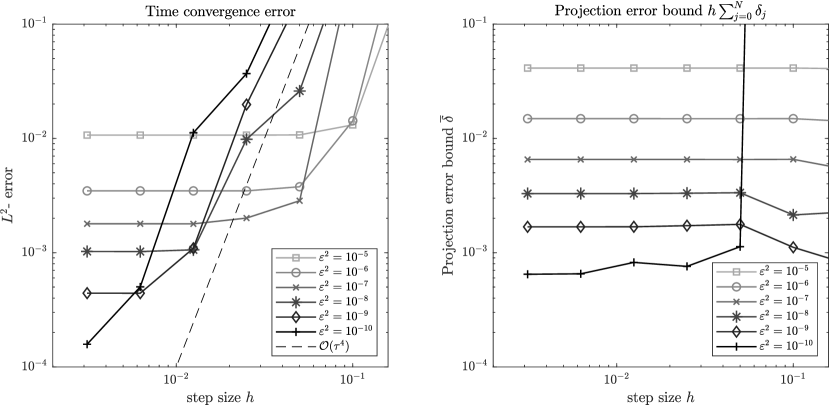
Figure 1: Time convergence plot for the Lotka–Volterra system, computed with a fixed neural network architecture with three hidden layers and four neurons each, which is fully described by $q\in\mathbb{R}^{62}$. We fix the regularization parameter $\varepsilon$ and observe the error behaviour of the classical Runge–Kutta approximation to the regularized flow (5). On the right-hand side, we plot the projection error term of the error bound described in Proposition 7.

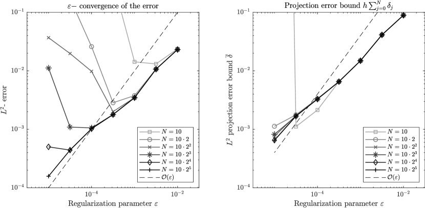
Figure 2: The $\varepsilon-$ convergence of the same network architecture, with the same time discretization. We fix the number of time steps and vary the regularization parameter.

9.2 Approximating double-well quantum dynamics

We consider a one-dimensional Schrödinger equation $\mathrm{i}\dot{\psi}=H\psi$ formulated within the setting of the complex Hilbert space ${\cal H}=L^{2}({\mathbb{R}},{\mathbb{C}})$. The equation serves as a model for tunneling dynamics. The Schrödinger operator

$$H=-\frac{1}{2}\partial_{x}^{2}+\alpha_{2}x^{2}+\alpha_{4}x^{4},\quad\psi_{0}(x)=\pi^{-1/4}{\mathrm{e}}^{-(x-q_{\ell})^{2}/2},$$

contains a quartic double-well potential with polynomial parameters $\alpha_{2}=-\frac{1}{8}$ and $\alpha_{4}=\alpha_{2}^{2}$. The initial condition $\psi_{0}$ is a single normalized Gaussian, whose width stems from the standard harmonic oscillator $H_{0}=-\frac{1}{2}\partial_{x}^{2}+\frac{1}{2}x^{2}$, placed at the left minimum $q_{\ell}=-2$ of the double well potential. During the time interval $[0,T]=[0,12]$ the wave packet travels from the left to the right well, see also Joubert24 . The approximation ansatz is a frozen sum of $M=36$ Gaussians,

$$u(t,x)=\sum_{m=1}^{M}c_{m}(t){\mathrm{e}}^{-x^{2}/2-\kappa_{m}(t)x},$$

with $2M$ complex parameters $\left(c_{m}(t),\kappa_{m}(t)\right)\in{\cal Q}={\mathbb{C}}^{2}$. For the initialization $u_{0}\in{\cal M}$, we put a non-uniform grid of Gauß–Hermite quadrature nodes $(x_{i},\xi_{j})$ with origin at $(q_{\ell},0)$ on ${\mathbb{R}}^{2}$, reformulate the corresponding Gaussian wave packets ${\mathrm{e}}^{-(x-x_{i})^{2}/2+\mathrm{i}\xi_{j}(x-x_{i})}$ in the complex algebraic format ${\mathrm{e}}^{-x^{2}/2-\kappa_{m}(0)x}$, and determine the optimal linear expansion coefficients $c_{m}(0)$ by solving the linear least squares problem

$$\left\|u(0)-\psi_{0}\right\|_{\cal H}=\min!$$

The matrices for the initial minimization and the ones involving the parameter Jacobian $\Phi^{\prime}(q)$ are evaluated via analytical formulas for Gaussian integrals of the type

$$\int_{\mathbb{R}}x^{k}{\mathrm{e}}^{-\beta x^{2}-\lambda x},\quad\beta>0,\quad\lambda\in{\mathbb{C}}.$$

The time integrator is the classical Runge–Kutta scheme of order four. As before, we observe the error behaviour for varying step size $h$ and regularization parameter $\varepsilon$.

In Figure 3, we fix several values of the regularization parameter $\varepsilon$ and vary the time step size $h$ to observe the time convergence behaviour. Since energy $\mathcal{E}(\psi(t))=\langle\psi(t),H\psi(t)\rangle_{\cal H}$, $t\in{\mathbb{R}}$, is a conserved quantity of the Schrödinger evolution, we evaluate the approximate energy $\mathcal{E}(u(t))$ at the final time $t=T$ and compare with the value at initial time $t=0$, see the left-hand side. We observe, that the simulations with the smallest regularization parameter $\varepsilon=10^{-5}$ have large errors and even prematurely terminate for the particular step size $h=4\cdot 10^{-3}$. For the other choices of the regularization parameter, the errors follow the order of the time integrator without the predicted step size restriction. On the right-hand side, we show the a posteriori error bounds for the projections. As before for the Lotka–Volterra model, these bounds are stable with respect to the time step size and estimate the accuracy of the underlying approximation.

In Figure 4, we conversely fix the size of the time step $h$ and present errors for a varying regularization parameter $\varepsilon$. The Schrödinger dynamics are unitary, and thus conserve the norm $\|\psi(t)\|_{\cal H}$, $t\in{\mathbb{R}}$, of the solution (mass conservation). On the left hand-side we compare the approximate norm $\|u(T)\|_{\cal H}$ at the final time $T$ with the exact unit value. We observe decay of the mass error only for relatively large values of the regularization parameter. Depending on the time step size, less regularization results in larger errors. The right-hand side shows the a posteriori terms of the error bound. Again, they capture the effects of the regularization parameter $\varepsilon$, but are by construction insensitive with respect to the time discretization.

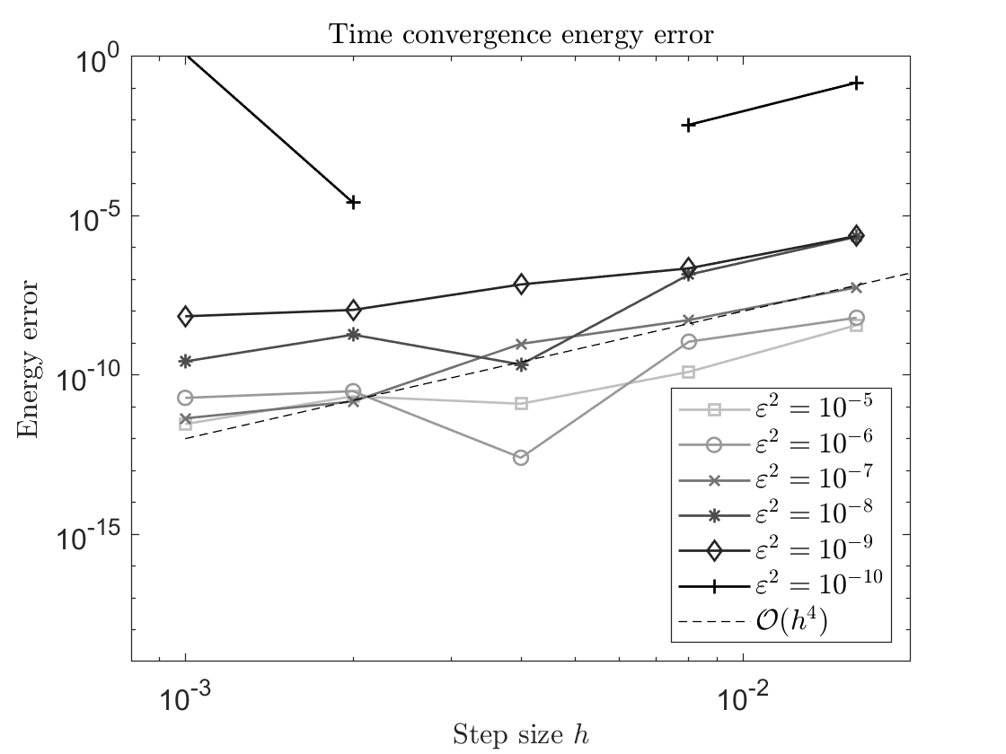
Figure 3: Time convergence plot for the double-well system, computed with a sum of $M=36$ complex Gaussians, which is fully described by $q\in\mathbb{C}^{72}$. We fix the regularization parameter $\varepsilon$ and observe the error behaviour of the classical Runge–Kutta approximation to the regularized flow (5). On the left-hand side, we plot the energy error $\left|\mathcal{E}(u(T))-\mathcal{E}(u(0))\right|$, on the right-hand side the projection error term of the error bound described in Proposition 7.

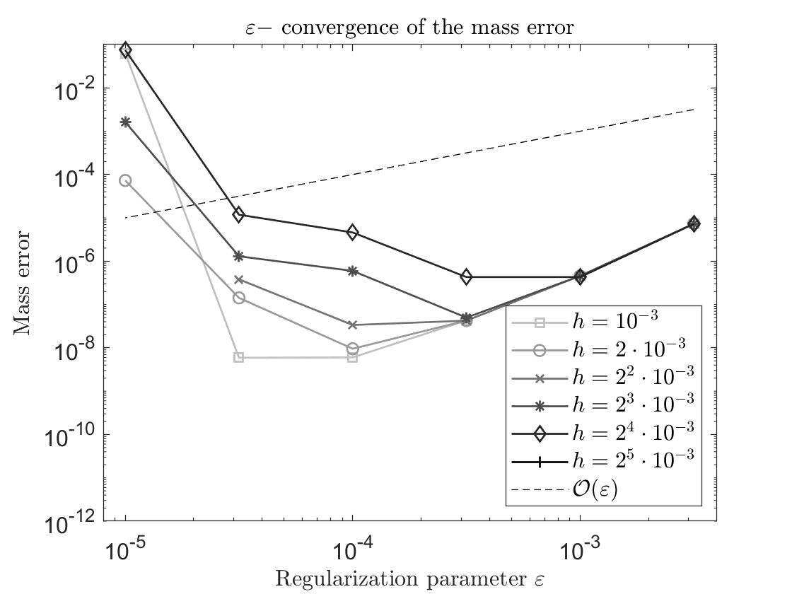
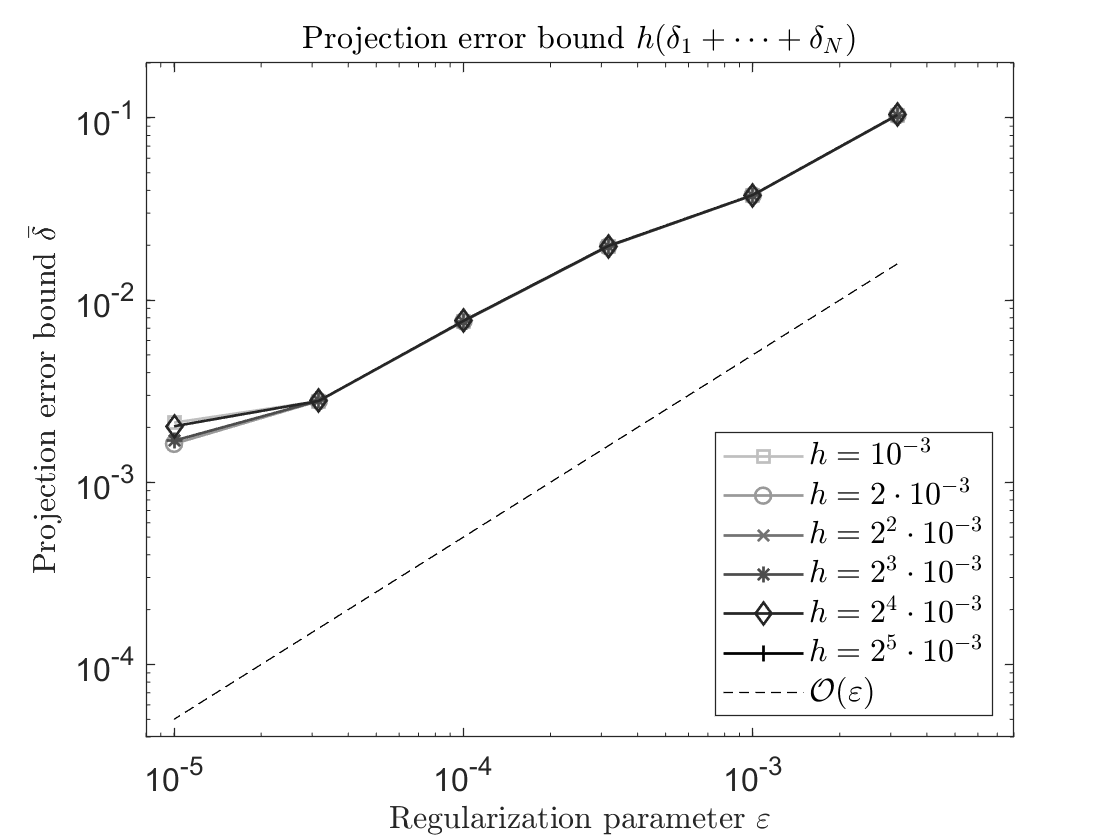
Figure 4: The $\varepsilon-$convergence of the same sum of Gaussians, with the same time discretization. We fix the number of time steps and vary the regularization parameter. On the left-hand side, we plot the norm error $|\|u(T)\|^{2}_{\cal H}-1|$, on the right-hand side the projection error.

Appendix A Appendix: Note on the regularized least squares problem

To study the sensitivity with respect to the regularization parameter, we consider the linear least squares problem to find $x=x(\alpha)$ such that

$$\vartheta(\alpha):=\|Ax-b\|^{2}+\alpha\|x\|^{2}\quad\text{ is minimal},$$

where we take the Euclidean norms. Note that $\vartheta=\delta^{2}$ and $\alpha=\varepsilon^{2}$ in the setting of the paper. The dependence of $\vartheta$ on $\alpha$ is remarkably simple.

Lemma 7

We have

$$\vartheta^{\prime}(\alpha)=\|x(\alpha)\|^{2}.$$

Moreover,

$$\vartheta^{\prime\prime}(\alpha)=\frac{d}{d\alpha}\|x(\alpha)\|^{2}\leq 0\quad\text{ and }\quad\frac{d}{d\alpha}\,\frac{\vartheta(\alpha)}{\alpha}\leq 0.$$

Proof

With $M=M(\alpha)=(A^{\top}A+\alpha I)$ we have the normal equations $Mx=A^{\top}b$ and hence

$$x=M^{-1}A^{\top}b.$$

Since $M^{\prime}=I$, we have $Mx^{\prime}+x=0$ and hence

$$x^{\prime}=-M^{-1}x.$$

We have

$$\vartheta^{\prime}=2\langle Ax-b,Ax^{\prime}\rangle+2\alpha\langle x,x^{\prime}\rangle+\|x\|^{2},$$

which becomes

$$\langle Ax-b,Ax^{\prime}\rangle=\langle Ax-b,-AM^{-1}x\rangle=-\langle x,A^{\top}AM^{-1}x\rangle+\langle M^{-1}A^{\top}b,x\rangle$$

$$=-\langle x,A^{\top}AM^{-1}x\rangle+\langle x,x\rangle=\langle x,(I-A^{\top}AM^{-1})x\rangle=\langle x,\alpha M^{-1}x\rangle,$$

and

$$\alpha\langle x,x^{\prime}\rangle=\langle x,-\alpha M^{-1}x\rangle,$$

so that

$$\vartheta^{\prime}=2\langle x,\alpha M^{-1}x\rangle+2\langle x,-\alpha M^{-1}x\rangle+\|x\|^{2}=\|x\|^{2},$$

which is the stated result for the first derivative. The second derivative is

$$\vartheta^{\prime\prime}=\frac{d}{d\alpha}\,\|x(\alpha)\|^{2}=2\langle x,x^{\prime}\rangle=-2\langle x,M^{-1}x\rangle,$$

which is negative (unless $x=0$), since $M$ is positive definite. Finally,

$$\left(\frac{\vartheta}{\alpha}\right)^{\prime}=\frac{\alpha\vartheta^{\prime}-\vartheta}{\alpha^{2}}=\frac{\alpha\|x\|^{2}-\vartheta}{\alpha^{2}}=-\frac{\|Ax-b\|^{2}}{\alpha^{2}},$$

which is non-positive. ∎

The following matrix estimates are often used in the paper.

Lemma 8

Denote $M_{\varepsilon}=A^{\top}A+\varepsilon^{2}I$. We have in the matrix 2-norm

$$\|AM_{\varepsilon}^{-1}A^{\top}\|\leq 1,\qquad\|AM_{\varepsilon}^{-1}\|\leq\frac{1}{2\varepsilon},\qquad\|M_{\varepsilon}^{-1}\|\leq\frac{1}{\varepsilon^{2}}.$$

Proof

The bounds follow from the singular value decomposition $A=U\Sigma V^{\top}$ with $U$ a linear isometry, $V$ unitary and $\Sigma$ diagonal. Then,

$$AM^{-1}A^{\top}=U\Sigma\left(\Sigma^{2}+\varepsilon^{2}I\right)^{-1}\Sigma U^{\top}.$$

Since $U$ is a linear isometry, we have

$$\|AM_{\varepsilon}^{-1}A^{\top}\| \leq\|\Sigma\left(\Sigma^{2}+\varepsilon^{2}I\right)^{-1}\Sigma\|\leq\ \sup_{\sigma\geq 0}\frac{\sigma^{2}}{\sigma^{2}+\varepsilon^{2}}=1.$$

Similarly, $AM^{-1}=U\Sigma(\Sigma^{2}+\varepsilon^{2}I)^{-1}U^{\top}$, so that

$$\|AM_{\varepsilon}^{-1}\| =\|\Sigma(\Sigma^{2}+\varepsilon^{2})^{-1}\|\leq\sup_{\sigma\geq 0}\frac{\sigma}{\sigma^{2}+\varepsilon^{2}}=\frac{1}{2\varepsilon},$$

and further

$$\|M_{\varepsilon}^{-1}\|=\|(\Sigma^{2}+\varepsilon^{2})^{-1}\|\leq\sup_{\sigma\geq 0}\frac{1}{\sigma^{2}+\varepsilon^{2}}=\frac{1}{\varepsilon^{2}},$$

as stated. ∎