Optimization hardness constrains ecological transients

Abstract

Living systems operate far from equilibrium, yet few general frameworks provide global bounds on biological transients. Here, we frame equilibration in complex ecosystems as the process of solving an analogue optimization problem. We show that functional redundancies among species in a complex foodweb lead to harder, ill-conditioned problems, manifesting as slow modes on a nearly-degenerate solution landscape. Common dimensionality reduction methods precondition ecological dynamics, by isolating fast relaxation from slow “solving” timescales that exhibit transient chaos for harder problem instances. In evolutionary simulations, we show that selection for steady-state diversity produces ill-conditioning, an effect quantifiable using complexity bounds for constrained optimization. Our results demonstrate the physical toll of computational constraints on biological dynamics.

Half a century ago, Robert May used random matrix theory to show that large, random ecosystems are typically unstable—defying conventional understanding of biodiversity, and suggesting that structural and evolutionary factors tune biological networks towards stable equilibria [1]. But how relevant is stability to real-world biological systems? In general, high-dimensional dynamical systems undergo extended excursions away from stable fixed points. For example, while fluid flow through a pipe possesses a globally-stable laminar state, small disturbances trigger transient turbulent excursions with expected lifetimes that increase rapidly with the flow speed [2].

Transient effects dominate many real-world foodwebs over experimentally-relevant timescales; examples include cyclic succession among rival vegetation species [3], turnover in patchy phytoplankton communities [4], and establishment of gut microbiota [5]. Theoretical works confirm that long-lived transients robustly appear in model foodwebs as the number of interacting species increases [6, 7, 8]. Transients may thus influence how many real-world ecosystems respond to exogenous perturbations [9], with implications for management and biodiversity [3]. However, analytical techniques primarily consider the effects of small perturbations from equilibrium points, leading to local characterization of transients in terms of quantities like reactivity or finite-time Lyapunov exponents [10, 11, 9, 12, 13]. Such approaches successfully predict experimental phenomena such as critical slowdown near tipping points in microbial ecosystems [14, 12], but they provide less insight into community assembly or large changes (e.g., crises) [15]. Recently, statistical approaches extend local measures by characterizing the distribution of fixed points in random ecosystems; these methods calculate the frequency and stability of local minima and marginally-stable equilibria, which act as kinetic traps that impede equilibration [16, 6, 17, 18, 19]. Statistical approaches also bound the set of valid solutions for a given ecosystem, thus providing null models against which to assess experimentally-observed communities [20, 21, 22]. However, few analytical approaches directly characterize the global dynamics of ecological transients, and it remains unknown whether universal, statistical bounds—analogous to the flow speed in turbulence—govern the onset of transients in ecological networks.

Here, we show that computational complexity measures from optimization theory govern the equilibration of ecological networks. We introduce a class of ill-conditioned ecosystems, for which functional redundancies control the rate of approach to equilibrium. The resulting optimization problem is difficult in a computational sense, and we show that this “excess computation” manifests as transient chaos associated with slow dynamical modes. Dimensionality reduction optimally preconditions the problem by separating fast relaxation from slow “solving” dynamics associated with redundant species. Using genetic algorithms, we evolve ecosystems to support higher steady-state diversity, which we find increases ill-conditioning and thus optimization hardness. Our results frame ecological dynamics through analogue optimization hardness, and show how computational constraints on biological systems produce physical effects.

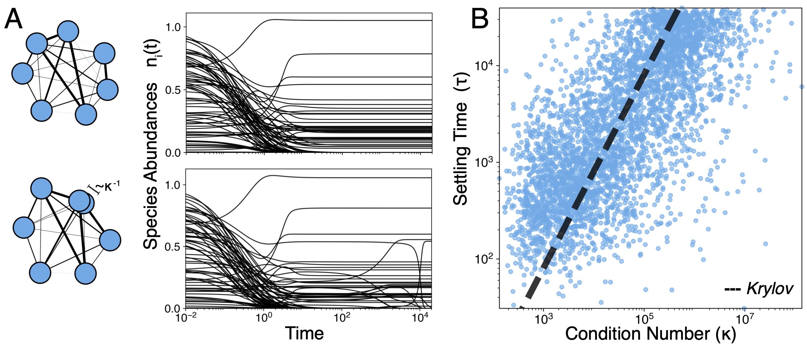
Figure 1: Long-lived transients in ill-conditioned ecosystems. (A) Equilibration of a biological network with random connectivity (top), and in a network perturbed to have functional near-redundancy (bottom). (B) Settling time $\tau$ versus condition number $\kappa$ for $10^{4}$ random communities; dashed line shows the scaling expected for an iterative linear program solver.

We introduce a class of random rank-deficient ecological networks based on the generalized Lotka-Volterra model,

$$\dot{n}_{i}(t)=n_{i}(t)\left(r_{i}+\sum_{j=1}^{N}A_{ij}n_{j}(t)\right)$$ (1)

where $n_{i}(t)$ refers to the abundance of species $i$ with intrinsic growth rate $r_{i}$. This species interacts with $N$ other species in the community through the matrix $A\in\mathbb{R}^{N\times N}$ encoding mutualistic ($A_{ij}>0$), neutral ($A_{ij}=0$), and competitive ($A_{ij}<0$) interactions.

We randomly sample $A$ from the family of matrices,

$$A=P^{T}(Q-d\,I)P+\epsilon\,E$$ (2)

where $Q_{ij},E_{ij},r_{i}\sim\mathcal{N}(0,1)$, $d$ is a density limitation constant, $\epsilon\ll 1$ is a small perturbation, and $I$ is the identity matrix. When $\epsilon=0$ and $P=I$, our formulation matches prior studies [23]. In this scenario, there exists a finite density limitation $d>0$ such that $A+A^{\top}$ is negative definite and thus Eq. 3 has a stable, non-invasible global equilibrium due to Lyapunov diagonal stability [24]. In this regime, Eq. 3 exhibits a relationship between stability and steady-state diversity as $N$ increases: the global fixed point $n_{i}(t)\rightarrow n_{i}^{*}$ has $n_{i}^{*}>0$ for $N_{\text{coex}}\leq N$ species, where across replicate random ecosystems $N_{\text{coex}}$ satisfies a binomial distribution with $\langle N_{\text{coex}}\rangle_{A}=N/2$ [23]. When sampling $A$ we additionally set $95\%$ of all interactions to zero, in order to mimic the low connectance ($C=0.05$) of real-world communities [25]; as in prior works, we find this condition does not affect our observed results as long as the connectance exceeds the percolation threshold ($C>1/N$)[23].

When $P\neq I$ and $\text{rank}(P)=M<N$, the rank-deficient matrix $P$ encodes functional redundancy between species in the population (Fig. 1A). Our approach reduces to a scenario considered in previous work when $P$ represents the identity matrix with the $j^{th}$ column duplicated at position $k$, implying that species $j$ and $k$ are functionally equivalent [17]. More generally, $P$ may encode arbitrary linear combinations of species that collectively substitute for others within the population. When $\epsilon=0$, a rank-deficient $P$ imposes multistability in Eq. 3, and each steady-state solution inhabits a continuous hyperplane of equivalent solutions containing varying mixtures of substitutable species. However, the singular perturbation $\epsilon>0$, $\epsilon\ll 1$ breaks symmetry among exact solutions and restores $\text{rank}(A)=N$, causing the system to regain a single global equilibrium $\mathbf{n}^{*}$. The resulting dynamics exhibit a slow timescale $\sim\!\epsilon^{-1}$ associated with final approach to equilibrium (Fig. 1A).

Functional redundancy in Eq. 3 differs from niche overlap because it arises from interspecific interchangability, rather than competition. Interaction-level redundancy leads to neutral community structure in experimental microbial ecosystems, where genetically-distinct groups can take on equivalent functional roles across replicates [26, 27]. Prior theoretical studies find that steady-state degeneracy due to functional redundancy can be broken by spatial effects, introducing slow dynamical modes associated with characteristic diffusion time (analogous to $\epsilon^{-1}$ in our model) [28]. In relation to other biological networks, we note that the perfectly-substitutable case $\epsilon\rightarrow 0$ implies that $A$ has $N-M$ repeated eigenvalues, equivalent to zero modes that arise in elastic models of allostery in biomolecules [29], as well as epistasis in genetic models [30]. In statistical learning theory, high-dimensional optimization landscapes have been found to exhibit linear mode connectivity, in which networks of zero-barrier connections bridge between optima [31], a concept extending earlier works describing symmetry-induced submanifolds that influence the dynamics of learning [32].

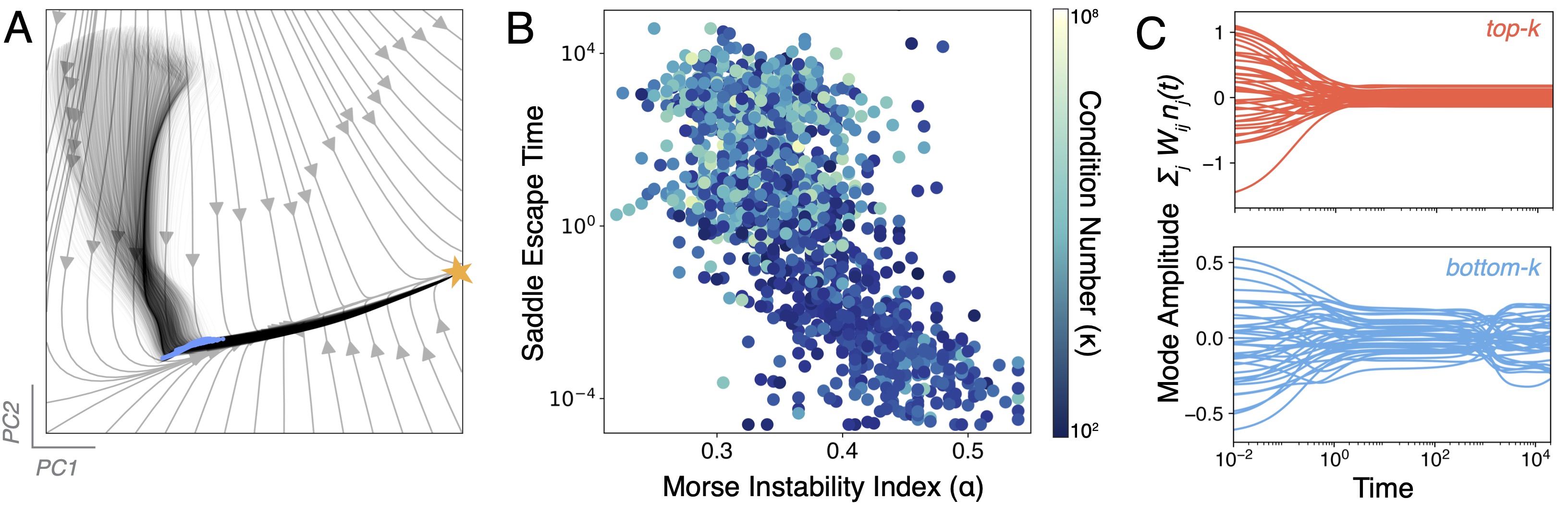
Figure 2: Slow manifolds create a complex optimization landscape. (A) An embedding of $10^{3}$ trajectories with different initial conditions in an ill-conditioned ecosystem ($\epsilon>0$). The global equilibrium is marked with a star, and the corresponding solutions of the degenerate ($\epsilon=0$) case are overlaid (blue). (B) Time that ill-conditioned trajectories for different random ecosystems (colored by condition number) spend near the former ($\epsilon=0$) solutions, versus the solution’s Morse instability index. (C) Projection of a single trajectory onto the right singular vectors associated with the largest (red) and smallest (blue) singular values.

To understand this effect, we note that the steady-state solution $\mathbf{n}^{*}$ solves the constrained linear regression $-A\mathbf{n}^{*}=\mathbf{r}$, $n_{i}^{*}\geq 0$. The Lotka-Volterra ecosystem model therefore solves an analogue linear programming problem; without density-dependence (the outermost $n_{i}(t)$ term), Eq. 3 would represent a linear time-invariant system. We thus hypothesize that the lifetime of transients relates to the difficulty of the underlying linear optimization problem, which is traditionally quantified by the condition number, $\kappa(A)\equiv\|A\|\|A^{-1}\|$. $\kappa\sim 10^{0}$ implies that $A$ may easily be inverted to solve for $\mathbf{n}^{*}$. As $\kappa\rightarrow\infty$, solving the system becomes more sensitive to small errors; the expected number of digits of required precision increases as $\sim\log_{10}\kappa$ [33].

We expect that ecosystems become ill-conditioned as species become harder to distinguish. We simulate the dynamics of $10^{4}$ random ecosystems with varying values of $\epsilon$, and find that ill-conditioned ecosystems generally take longer to equilibrate, as measured by the settling time $\tau$ that it takes a trajectory to first fall within a fixed radius $\xi\ll 1$ of $\mathbf{n}^{*}$ (Fig. 1B). In numerical analysis, iterative solution of linear programs exhibits a known bound on convergence time $\tau=\log{\xi}/\log[(\kappa-1)/(\kappa+1)]$ (Fig 1B, dashed line) [33]. We find that this bound coincides with the scaling of settling in random ecosystems, underscoring the physical effects of ill-conditioning in our system. Rather than a purely numerical consideration, $\kappa$ is a physical quantity that can be interpreted as a measure of computational complexity or inverse distance to an ill-conditioned (here, degenerate) problem [34]. As a result, despite the heterogeneity of the various random ecosystems in Fig. 1B, the quantity $\kappa$ imposes a global constraint on equilibration time.

We analyze the physical origin of ill-conditioning by embedding the $N=10^{3}$-dimensional dynamics in two dimensions using principal components analysis (Fig. 2A, black traces). We find that trajectories emanating from diverse initial conditions become trapped along a low-dimensional manifold. Reintegrating each trajectory at $\epsilon=0$ confirms that this manifold represents the degenerate solution space, which becomes a trapping region when $\epsilon>0$ (Fig. 2A, blue points). After escaping these slow regions, trajectories approach the global fixed point. Slow transients due to unstable solutions have previously been characterized in complex foodwebs [3], and they particularly arise in systems with cyclic dominance and succession [4]. In statistical learning theory, optimization of random high-dimensional landscapes is often dominated by saddle points, which become exponentially more likely than local minima as problem dimensionality grows [35]. Recent theoretical results confirm this effect for Eq. 3 in the well-conditioned ($P=I$) limit: as the number of species grows, the system spends more time trapped near saddles [7, 36, 37, 18].

Because our formulation Eq. 3 contains manifolds of unstable solutions induced by the symmetry-breaking perturbation $\epsilon$, we consider the role to which these pseudosolution manifolds globally shape the dynamics. Recent work on low-rank structure in large datasets ties low effective dimensionality to the structure of underlying interaction networks [38]. We note that any interaction matrix $A$ has a real-valued singular value decomposition of the form $A=U\Sigma V^{\top}$, where the diagonal matrix $\Sigma\in\mathbb{R}^{N\times N}$ contains the singular values $\sigma_{i}$ of $A$ in decreasing order along its main diagonal [33]. For our interaction matrix Eq. 4, Weyl’s inequality $|\sigma(A)_{i}-\sigma(A-\epsilon E)_{i}|\leq\epsilon\sqrt{C\,N}$ entails that $A$ is nearly low-rank, with $N-M$ singular values $\sim\epsilon$ [38]. Globally, this means that the $N$-dimensional dynamics are dominated by $M$ dimensional slow manifolds. These slow modes (formerly stable solutions in the $\epsilon=0$ case) are misaligned across phase space, leading to a separation between gradual dynamics on slow modes, and fast high-dimensional transitions among them. On a given mode $\mathbf{n}^{*}$, we perform a matched expansion of Eq. 3 in terms of $\epsilon$ and a small perturbation off the slow manifold $\mathbf{n}(t)=\mathbf{n}^{*}+\delta\mathbf{n}(t)$, producing the linearized dynamics $\dot{\delta}\mathbf{n}(t)=\mathbf{n}^{*}\odot(A\delta\mathbf{n}(t)+\epsilon E\mathbf{n}^{*})$. The first term constitutes the Jacobian of the unperturbed case ($J_{ij}\equiv n_{i}^{*}A_{ij}$), commonly known as the community matrix [15]. The second term prevents equilibration by inducing slow $\sim\!\epsilon$ drift along the manifold. To quantify kinetic trapping, we numerically identify slow manifolds for each of the random ecosystems shown in Fig. 1B, and compute its scaled Morse instability index, $\alpha\equiv N^{-}/N$, the relative number of unstable “escape” directions $N^{-}\leq N$ emanating from a given saddle region $\mathbf{n}^{*}$ based on the eigenvalue spectrum of $J$. Saddles with relatively few downwards directions ($0<\alpha\ll 1$) generally take longer to escape. We confirm this effect by directly measuring the escape time for each pseudosolution (Fig. 2B). The escape time linearly decreases with $\alpha$ across different ecosystems, consistent with theoretical expectations for hyperbolic systems [39].

Recent works coarse-grain large ecosystems through collective “ecomodes,” or groups of species that act in concert [40, 17]. We thus consider linearly projected dynamics $W\mathbf{n}(t)$, where $\dim(W\mathbf{n})<\dim(\mathbf{n})$. The projected dynamics are governed by $W\circ\mathbf{F}(\mathbf{n})$, with $\mathbf{F}$ given by Eq. 3, and we presume the existence of a dynamical system in the projected coordinates $\mathbf{f}(W\circ\mathbf{n})$. Recent results for low-rank systems show that the choice of operator $W=\hat{V}^{\top}$ minimizes the least-squares alignment error between $W\circ\mathbf{F}$ and $\mathbf{f}\circ W$ in a $K$-dimensional projection, where the columns of $\hat{V}$ contain the $K$ leading right singular vectors $V$ in the singular value decomposition of $A$. We thus define two projections $W_{\text{fast}}=V_{:,1:K}$ and $W_{\text{slow}}=V_{:,(N-K+1):N}$, and map an example ill-conditioned ecosystem’s trajectory onto them in Fig 2C. $W_{\text{fast}}\mathbf{n}(t)$, $W_{\text{slow}}\mathbf{n}(t)$ reveal separate fast timescales for relaxation onto to the slow manifold network, and slow ($\sim\kappa$) timescales associated with navigating these modes (Fig. 2C).

In large-scale optimization, ill-conditioning may be mitigated if a transformation $-WA\mathbf{n}=W\mathbf{r}$ satisfies $\kappa(WA)\ll\kappa(A)$. For our system, we observe that both $W_{\text{fast}}$ and $W_{\text{slow}}$ effectively precondition the dynamics, with $\kappa(W_{\text{fast}}A)/\kappa(A)<10^{-4}$ and $\kappa(W_{\text{slow}}A)/\kappa(A)<10^{-5}$. In general, $\kappa(A)=\sigma_{\text{max}}(A)/\sigma_{\text{min}}(A)$, and so projections precondition primarily by reducing the number of singular values, and thus range of timescales. Preconditioning is known to isolate fast and slow subspaces in iterative linear solvers [33], and our findings connect this phenomenon to the empirical success of dimensionality reduction in describing high-dimensional foodwebs, especially microbial ecosystems [40, 17, 26]. When $A$ is symmetric, our preconditioning argument supports prior works that construct ecomodes using eigenvectors of the interaction matrix [17]. These works also find soft modes associated with degenerate eigenvalues, which identify substitutable species and thus the rank (effective size) of an ecosystem [17]. However, because the eigenvectors of a non-symmetric matrix have no general relationship with the right singular vectors, the projection $V^{\top}$ should be preferred for systems with non-reciprocal (e.g. predator-prey or consumer-resource) interaction.

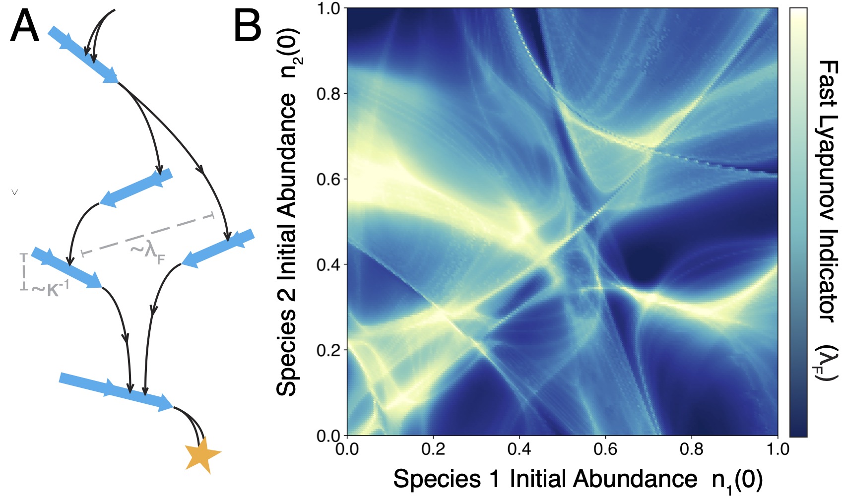
Figure 3: Transient chaos due to slow manifold scattering. (A) The “pachinko” mechanism for ill-conditioned dynamics, in which slow manifolds temporarily disperse neighboring trajectories that later reunite at the global equilibrium. (B) Caustics in the Fast Lyapunov Indicator ($\lambda_{F}$) versus initial conditions on a two-dimensional slice through the $N$-dimensional space of initial species densities.

Random ill-conditioned ecosystems prove harder to solve due to the need to navigate the slow manifold network, suggesting that such systems pose more computationally-demanding optimization problems. But where is this excess computation allocated? A variant of the Church-Turing thesis for analogue computing asserts that continuous simulation of a hard combinatorial optimization problem likely incurs exponential cost [41]. Recent continuous formulations of discrete constraint satisfiability problems show that hard problem instances exhibit transient chaos, which manifests as exponentially-increasing sensitivity (and thus required precision) and fractal basin boundaries across initial conditions [42]. For our system, we surmise that the slow manifolds act analogously to constraints, producing an irregular landscape of slow barriers that temporarily scatter trajectories as they approach the global fixed point, a mechanism reminiscent of a pachinko game (Fig. 3A). To formalize this intuition, we compute the fast Lyapunov indicator ($\lambda_{F}$), a quantity originally developed by astrophysicists to quantify the stability of planetary orbits in high dimensions [43]. For each trajectory $\mathbf{x}(t)$ of Eq. 3, we integrate the variational equation $\dot{\mathbf{w}}(t)=\mathbf{J}[\mathbf{x}(t)]\mathbf{w}(t)$, where $\mathbf{w}(0)=I\in\mathbb{R}^{N\times N}$. The quantity $\lambda_{F}=\max_{t}\log\|\mathbf{w}(t)\|_{2}$ captures the maximum chaoticity encountered on a trajectory, a quantity more informative than the true Lyapunov exponents for transient dynamics where $\lim_{t\rightarrow\infty}\log\|\mathbf{w}(t)\|_{2}/t=0$. We note that $\lambda_{F}$ represents a nonlinear generalization of the power method, a standard iterative technique for finding the largest eigenvalues of square matrices [33]. We therefore interpret $\lambda_{F}$ as a spatially-resolved probe of the local conditioning of $A$ for a given initialization $\mathbf{n}(0)$. A random two-dimensional slice through the space of initial species densities reveals intricate pseudobasins, indicating abrupt changes in the route by which the ecosystem approaches to equilibrium when initial species densities change by small amounts (Fig. 3B). These patterns resemble optical caustics, which arise when density fluctuations in a transparent medium distort the pathlengths of light rays. Here, the slow manifolds play a similar role by intermittently trapping and scattering trajectories arising from different initial conditions. We note that this slow-mode mechanism differs from the scrambling induced by chaotic saddles in high-dimensional open chaotic systems like planetary orbits [43, 44]; rather, our system resembles doubly-transient chaos, a recently-characterized phenomenon in dissipative systems that approach global fixed points by differing routes [45].

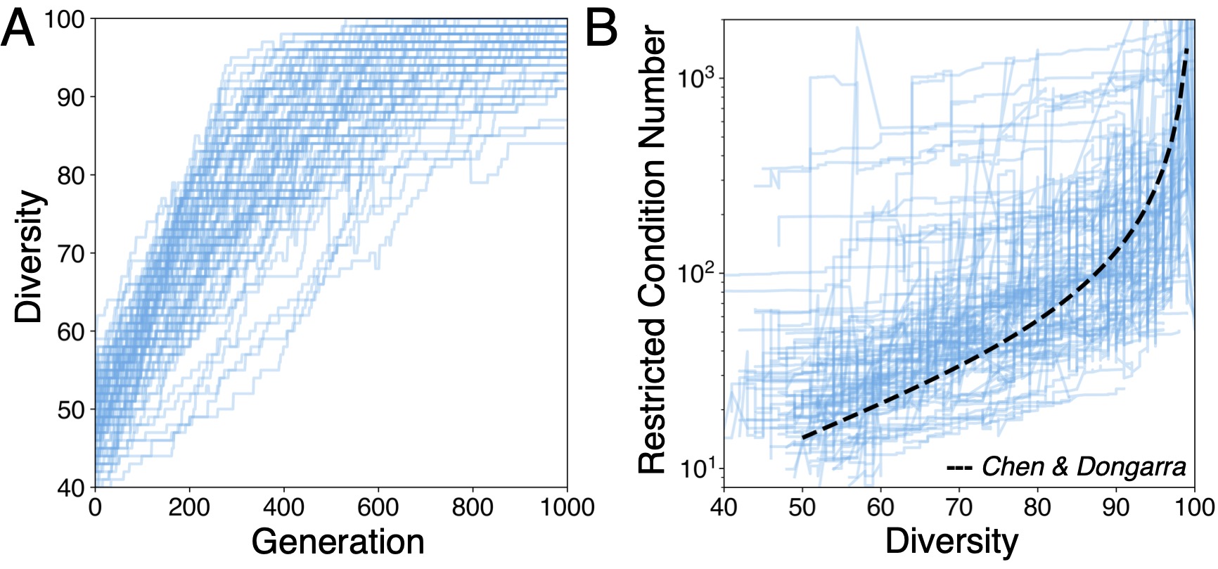
Figure 4: Selection for diversity produces ill-conditioning. (A) Condition number versus generation for $10^{3}$ replicate random communities of $N=10^{3}$ species evolved to have high steady-state diversity. (B) The condition number of the minor matrix associated with species that survive at steady-state, versus the overall steady-state diversity. Dashed line indicates expected condition number for a random $N\times N_{\text{coex}}$ Gaussian matrix.

We conclude by considering whether ill-conditioning can influence non-random interaction networks encountered in real ecosystems. We use a genetic algorithm to evolve random foodwebs by selecting for increased steady-state diversity $N_{\text{coex}}$. In our procedure, we randomly sample $10^{3}$ distinct well-conditioned random foodwebs ($P=I$), and simulate their dynamics until they reach steady state $\mathbf{n}^{*}$. We select the 10% of foodwebs with highest $N_{\text{coex}}\equiv\|\mathbf{n}^{*}\|_{0}$ to propagate to the next generation, and we cull the remaining $90\%$ and replace them with new foodwebs assembled from random blocks of row-column pairs sampled from the top $10\%$. We repeat this procedure for $10^{3}$ generations.

We find that evolving foodwebs towards higher $N_{\text{coex}}$ robustly produces higher-$\kappa$ states, independently of foodweb scale, crossover rates, or inclusion of mutation in the genetic algorithm (Fig. 4A). The robust emergence of ill-conditioning implies that an intrinsic physical tradeoff, rather than a dynamical effect, produces the observed scaling. Intuitively, as $N_{\text{coex}}$ increases, fewer positivity constraints in Eq. 3 remain active at equilibrium, and so the system becomes less constrained. We thus consider the condition number $\hat{\kappa}$ of the minor matrix comprising only the columns of $A$ associated with nonzero entries in $\mathbf{n}^{*}$. Principal minors of a positive definite matrix remain positive definite, and so the reduced system retains a global fixed point. Computing $\hat{\kappa}$ for varying $N_{\text{coex}}$ confirms a general relationship (Fig. 4B), which closely follows a known scaling law for the condition number of a random rectangular matrix, $\hat{\kappa}=9.563\,N/(N-N_{\text{coex}}+1)$ (dashed line) [46]. This suggests that ill-conditioning arises primarily from diversity, and not fine-tuned interaction values. Physically, this effect represents species packing: adding new species to an ecosystem increases the probability of duplicating an existing function. From an optimization standpoint, there are two competing effects: as $N_{\text{coex}}$ increases, fewer non-negativity constraints remain active, but the probability that two species are redundant increases. This interplay is known complementary slackness in constrained optimization contexts [33]. Consistent with this interpretation, recent works map consumer-resource models (which generalize Eq. 3) onto quadratic optimization programs [16] and constraint satisfaction problems [21], and find that niche overlap may be understood as redundancy emerging at high constraint loads.

Drawing on recent work in transient chaos and optimization theory, we have shown that equilibration of random food webs is globally constrained by ill-conditioning. While our analysis largely relies on the particular form of Eq. 3 as an analogue constrained linear regression, we emphasize that $\kappa$ physically represents the inverse distance to a singular problem (here, functional redundancy), and thus the computational cost to solve a linear system. In optimization theory, a generalized condition number exists, in principle, for any constraint problem in terms of the distance to singularity within the feasible solution set [47]. For example, in random Boolean satisfiability problems, the effective conditioning is governed by the ratio of constraints to variables [42]. While direct calculation of generalized condition number is prohibitive for many problem classes, it suggests that global computational constraints on equilibration exist for more complicated foodweb models, or other types of biological networks. Our work thus provides a tractable example of how intrinsic computational complexity may influence the organization of a biological system.

I Acknowledgements

W.G. thanks Annette Ostling and Yuanzhao Zhang for informative discussions. Computational resources for this study were provided by the Texas Advanced Computing Center (TACC) at The University of Texas at Austin. This project has been made possible in part by grant number DAF2023-329596 from the Chan Zuckerberg Initiative DAF, an advised fund of Silicon Valley Community Foundation.

II Code Availability

Code for this study is available at https://github.com/williamgilpin/illotka

III Slow modes in the Generalized Lotka-Volterra model.

The generalized Lotka-Volterra model has the form,

$$\dot{n}_{i}(t)=n_{i}(t)\left(r_{i}+\sum_{j=1}^{N}A_{ij}n_{j}(t)\right),$$ (3)

The growth rates $r_{i}\sim\mathcal{N}(0,1)$ include species capable of growing in isolation ($r_{i}>0$, such as autotrophs) and those that require other species to survive $r_{i}<0$. The matrix $A$ is sampled from the family of matrices,

$$A=P^{T}(Q-d\,I)P+\epsilon\,E.$$ (4)

$Q_{ij},E_{ij}\sim\mathcal{N}(0,1)$, $\epsilon\ll 1$, $d$ is a density-limitation constant, and $I$ is the identity matrix. We introduce the notation $A=A^{(0)}+\epsilon\,E$, where $A^{(0)}\equiv P^{T}(Q-d\,I)P$. We linearize Eq. 3 around a slow manifold $\mathbf{n}^{*}$, such that $\mathbf{n}(t)=\mathbf{n}^{*}+\delta\mathbf{n}(t)$ and $-A^{(0)}\mathbf{n}^{*}=\mathbf{r}$. Matching terms of equivalent order results in linearized dynamics

$$\dot{\delta n}_{i}(t)=n_{i}^{*}\sum_{j=1}^{N}A^{(0)}_{ij}\,\delta n_{j}(t)+\epsilon\,n_{i}^{*}\sum_{j=1}^{N}E_{ij}\,n_{j}^{*}$$ (5)

where we have discarded terms $\sim\!\mathcal{O}(\delta n_{i}\delta n_{j})$ and $\sim\!\mathcal{O}(\epsilon\delta n_{i})$. We note that retaining the latter terms would lead to perturbations $\sim\!\mathcal{O}(\epsilon)$ to the eigenvalues of the unperturbed Jacobian; however, in the globally-stable regime, the dynamics near the equilibrium point are dominated by the density-dependent term $d$, and so these cross-terms have minor effects on the global fixed point.

The first term in Eq. 5 creates linearized dynamics described by the unperturbed Jacobian matrix (community matrix) [48]. The unperturbed Jacobian matrix may be alternatively written as the matrix product $A\;\text{diag}(\mathbf{n}^{*})$, and it is independent of $\epsilon$. The second term biases the dynamics away from the unperturbed fixed point $\mathbf{n}^{*}$, creating a flow with speed $\sim\!\epsilon$ along the slow manifolds.

IV Numerical Integration.

All numerical results are generated with an implicit embedded Runge-Kutta solver (Radau) that inverts the analytic Jacobian at each timestep. Relative and absolute tolerances of the solver are set to $<10^{-12}$, ensuring accuracy comparable to recent studies of transient chaos [49, 45].

For calculation of the settling time, we numerically integrate until $\dot{\mathbf{n}}(t)<10^{-14}$, and we then use the eigenvalues of analytical Jacobian of Eq. 3 to confirm that the asymptotic value is a local minimum, which we consider an estimate of the global solution $\mathbf{n}^{*}$. We then use a nonnegative least-squares solver (the Lawson-Hanson algorithm implemented in scipy.optimize.nnls) to directly verify that $-A\mathbf{n}^{*}=\mathbf{r}$. We then retroactively find the settling time $\tau$ by choosing the fixed convergence floor $\xi=10^{-7}$ and find $\tau\equiv\inf_{t}(\|\mathbf{n}(t)-\mathbf{n}^{*}\|_{2}\leq\xi)$. The precision floors are chosen so that, in all cases, $\tau$ occurs before the termination of integration.

V Calculation of the Fast Lyapunov Indicator.

For calculation of the Fast Lyapunov Indicator (FLI), the variational equation $\dot{\mathbf{w}}(t)=J[\mathbf{n}(t)]\mathbf{w}(t)$, $\mathbf{w}(0)=I$ is introduced based on the analytic Jacobian of Eq. 3. The variational equation is integrated concurrently with the original trajectory, with all timesteps controlled by the implicit integration of $\mathbf{n}(t)$. During integration, whenever $\|\mathbf{w}(t)\|_{2}$ grows too large for numerical stability, we rescale all matrix elements and then store the scale factor, allowing the exact value of $\|w(t)\|_{2}$ to be reconstructed post hoc. For a given initial condition $\mathbf{n}(0)$, the Fast Lyapunov Indicator is given by

$$\lambda_{F}=\max_{t}\log\|\mathbf{w}(t)\|_{2}$$

where the $\mathbf{w}(t)\in\mathbb{R}^{N\times N}$ and $\mathbf{w}(0)=I$ [50]. The variational equation may be interpreted as evolving each column of $\mathbf{w}(t)$ separately. Because each column points in a different initial direction, the columns stretch at different rates depending on whether they happen to align with the initial stretching directions of $J(\mathbf{n}(t))$. At long times, the fastest-growing column dominates the matrix norm. $\lambda_{F}$ may thus be interpreted as the fastest exponential divergence observed at any time, and along any initial direction, for a given point $\mathbf{n}(0)$ in the domain of a dynamical system. This property contrasts $\lambda_{F}$ with the true Lyapunov exponent $\lim_{t\rightarrow\infty}\log\|\mathbf{w}(t^{\prime})\|/t$, which vanishes for most initial conditions for systems dominated by scattering or transient events. Prior works have shown that $\lambda_{F}$ can robustly detect transient events unfolding over a range of timescales, including short-period scrambling events in the restricted three-body problem [51], long-timescale resonances in the solar system [52, 53], and gradual diffusion in quasi-integrable Hamiltonian systems [43].

VI Embedding the slow manifold dynamics.

We fix the parameters of an ecosystem Eq. 3, with $\mathbf{F}(\mathbf{n};A,\mathbf{r})$ denoting the right hand side of the differential equation. We compute a set of $N_{\text{traj}}$ simulations originating from different initial conditions and sampled at $T$ discrete timepoints, $\mathbf{X}_{\text{traj}}\equiv\{\mathbf{n}^{(k)}(t)\}\in\mathbb{R}^{N_{\text{traj}}\times T\times N}$. On this set of trajectories, we perform principal components analysis (PCA) and transform the data into the full principal components space $\mathbf{Y}_{\text{pca}}\in\mathbb{R}^{N_{\text{traj}}\times T\times N}$. For visualization purposes, we truncate this matrix in order to visualize the trajectories along only the top two principal components, $\hat{\mathbf{Y}}_{\text{pca}}\in\mathbb{R}^{N_{\text{traj}}\times T\times 2}$. For each initial condition, we perform a replicate integration with $\epsilon=0$ in order to identify the set of fixed points for the degenerate case, $\mathbf{X}_{\text{traj}}^{(0)*}\in\mathbb{R}^{N_{\text{traj}}\times N}$. We project these unperturbed solutions into the PCA coordinates, in order to visualize in low dimensions the locations of formerly-stable solutions, $\hat{\mathbf{Y}}_{\text{pca}}^{(0)*}\in\mathbb{R}^{N_{\text{traj}}\times 2}$.

To obtain a vector field and streamlines, we define a uniform mesh over the first two PCA embedding coordinates $\hat{\mathbf{Y}}_{\text{mesh}}\in\mathbb{R}^{N_{\text{mesh}}\times 2}$, which we then promote to a full-dimensional mesh by appending the mean of the remaining $(N-2)$ PCA coordinates, producing the coordinates $\mathbf{Y}_{\text{mesh}}\in\mathbb{R}^{N_{\text{mesh}}\times N}$. We then invert the PCA transformation (a linear transformation and a shift by the featurewise mean vector) in order to pull $\mathbf{Y}_{\text{mesh}}$ back into the ambient coordinates $\mathbf{X}_{\text{mesh}}\in\mathbb{R}^{N_{\text{mesh}}\times N}$. In the inverted mesh coordinates, we evaluate Eq. 3 to produce a velocity vector field $\mathbf{U}=\mathbf{F}(\mathbf{X}_{\text{mesh}};A,\mathbf{r})\in\mathbb{R}^{N_{\text{mesh}}\times N\times N}$ in the ambient coordinates, which we then project back into the reduced-order PCA basis $\hat{\mathbf{V}}\in\mathbb{R}^{N_{\text{mesh}}\times 2\times 2}$ in order to visualize the vector field and streamlines along the slow manifold. We note that trajectories in the embedded coordinates may appear to cross streamlines, because the observed dynamics are a projection of higher-dimensional trajectories from a velocity field $\mathbf{V}\in\mathbb{R}^{N_{\text{mesh}}\times N\times N}$, where streamlines do not cross.

VII Evolutionary simulations

We randomly sample $10^{3}$ random interaction matrices with $P=I$, $\epsilon=0$ in Eq. 4. We integrate their dynamics under Eq. 3, using the same integration precision and termination conditions described in IV. Consistent with prior results [23], we observe that the initial steady-state diversity, $N_{\text{coex}}\equiv\|\mathbf{n}^{*}\|_{0}$, exhibits a binomial distribution across replicates, with $\langle N_{\text{coex}}\rangle_{A}\approx N/2$.

We next select the top $10\%$ of foodwebs ($A$ matrices) to survive to the next generation, and we delete the remaining $90\%$. We replace these culled foodwebs with new foodwebs with interactions randomly sampled from the surviving foodwebs. However, we hold constant the vector $\mathbf{r}$ of growth rates for each species. This is because the individual growth rates are the only distinguishing characteristic that would allow for distinct niches among the different species; if growth rates also evolve during the simulation, the system will trivially collapse onto a degenerate space of identical species in equal proportions. This case would be consistent with our observation that functional redundancy (and thus ill-conditioning) emerges at high diversity, but it otherwise provides little mechanistic insight.

We have also considered variants of our evolutionary procedure, including the addition of random mutations, constraints on crossover due to clamped values of the sparsity and norm of each $A$, and a more gradual recombination procedure, in which low-fitness ecosystems are not culled, but rather only partially updated based on interactions found in high-diversity ecosystems. While these hyperparameters affect evolution rate and convergence time, they have no effect on the scalings and tradeoffs we observe, suggesting that the phenomenon represents an intrinsic property of the space of ecosystems and $A$ matrices, rather than an artifact of our particular matrix sampling procedure.

From a biological perspective, we note that our approach represents a limiting case of eco-evolutionary dynamics, in which population dynamics proceed rapidly compared to evolutionary dynamics. Interestingly, while the population dynamics represent an optimization in the sense of solving a non-negative least-squares problem, the process of evolving the $A$ matrices with genetic algorithms represent a higher-level meta-optimization,

$$\underset{A}{\text{maximize}} \|\mathbf{n}^{*}\|_{0}$$

subject to $$-A\mathbf{n}^{*}=\mathbf{r},$$

$$n_{i}^{*}\geq 0,\;\forall i.$$

where the population dynamics are now encoded within an equality constraint.

References

- May [1972] Robert M May. Will a large complex system be stable? Nature, 238(5364):413–414, 1972.
- Avila et al. [2023] Marc Avila, Dwight Barkley, and Björn Hof. Transition to turbulence in pipe flow. Annual Review of Fluid Mechanics, 55:575–602, 2023.
- Hastings et al. [2018] Alan Hastings, Karen C Abbott, Kim Cuddington, Tessa Francis, Gabriel Gellner, Ying-Cheng Lai, Andrew Morozov, Sergei Petrovskii, Katherine Scranton, and Mary Lou Zeeman. Transient phenomena in ecology. Science, 361(6406):eaat6412, 2018.
- Morozov et al. [2020] Andrew Morozov, Karen Abbott, Kim Cuddington, Tessa Francis, Gabriel Gellner, Alan Hastings, Ying-Cheng Lai, Sergei Petrovskii, Katherine Scranton, and Mary Lou Zeeman. Long transients in ecology: Theory and applications. Physics of Life Reviews, 32:1–40, 2020.
- Schlomann and Parthasarathy [2019] Brandon H Schlomann and Raghuveer Parthasarathy. Timescales of gut microbiome dynamics. Current opinion in microbiology, 50:56–63, 2019.
- de Pirey and Bunin [2024] Thibaut Arnoulx de Pirey and Guy Bunin. Many-species ecological fluctuations as a jump process from the brink of extinction. Physical Review X, 14(1):011037, 2024.
- Ben Arous et al. [2021] Gérard Ben Arous, Yan V Fyodorov, and Boris A Khoruzhenko. Counting equilibria of large complex systems by instability index. Proceedings of the National Academy of Sciences, 118(34):e2023719118, 2021.
- Chen and Cohen [2001] Xin Chen and Joel E Cohen. Transient dynamics and food–web complexity in the lotka–volterra cascade model. Proceedings of the Royal Society of London. Series B: Biological Sciences, 268(1469):869–877, 2001.
- Neubert and Caswell [1997] Michael G Neubert and Hal Caswell. Alternatives to resilience for measuring the responses of ecological systems to perturbations. Ecology, 78(3):653–665, 1997.
- Snyder [2010] Robin E Snyder. What makes ecological systems reactive? Theoretical population biology, 77(4):243–249, 2010.
- Townley et al. [2007] Stuart Townley, David Carslake, Owen Kellie-Smith, Dominic McCarthy, and David Hodgson. Predicting transient amplification in perturbed ecological systems. Journal of Applied Ecology, pages 1243–1251, 2007.
- Tang and Allesina [2014] Si Tang and Stefano Allesina. Reactivity and stability of large ecosystems. Frontiers in Ecology and Evolution, 2:21, 2014.
- Suweis et al. [2015] Samir Suweis, Jacopo Grilli, Jayanth R Banavar, Stefano Allesina, and Amos Maritan. Effect of localization on the stability of mutualistic ecological networks. Nature communications, 6(1):10179, 2015.
- Dai et al. [2012] Lei Dai, Daan Vorselen, Kirill S Korolev, and Jeff Gore. Generic indicators for loss of resilience before a tipping point leading to population collapse. Science, 336(6085):1175–1177, 2012.
- Hastings and Wysham [2010] Alan Hastings and Derin B Wysham. Regime shifts in ecological systems can occur with no warning. Ecology letters, 13(4):464–472, 2010.
- Mehta et al. [2019] Pankaj Mehta, Wenping Cui, Ching-Hao Wang, and Robert Marsland III. Constrained optimization as ecological dynamics with applications to random quadratic programming in high dimensions. Physical Review E, 99(5):052111, 2019.
- Tikhonov [2017] Mikhail Tikhonov. Theoretical microbial ecology without species. Physical Review E, 96(3):032410, 2017.
- Biroli et al. [2018] Giulio Biroli, Guy Bunin, and Chiara Cammarota. Marginally stable equilibria in critical ecosystems. New Journal of Physics, 20(8):083051, 2018.
- Blumenthal et al. [2024] Emmy Blumenthal, Jason W Rocks, and Pankaj Mehta. Phase transition to chaos in complex ecosystems with nonreciprocal species-resource interactions. Physical Review Letters, 132(12):127401, 2024.
- Tikhonov and Monasson [2017] Mikhail Tikhonov and Remi Monasson. Collective phase in resource competition in a highly diverse ecosystem. Physical review letters, 118(4):048103, 2017.
- Altieri and Franz [2019] Ada Altieri and Silvio Franz. Constraint satisfaction mechanisms for marginal stability and criticality in large ecosystems. Physical Review E, 99(1):010401, 2019.
- Goyal et al. [2024] Akshit Goyal, Jason W Rocks, and Pankaj Mehta. A universal niche geometry governs the response of ecosystems to environmental perturbations. bioRxiv, pages 2024–03, 2024.
- Serván et al. [2018] Carlos A Serván, José A Capitán, Jacopo Grilli, Kent E Morrison, and Stefano Allesina. Coexistence of many species in random ecosystems. Nature ecology & evolution, 2(8):1237–1242, 2018.
- MacArthur [1970] Robert MacArthur. Species packing and competitive equilibrium for many species. Theoretical population biology, 1(1):1–11, 1970.
- Dunne et al. [2002] Jennifer A Dunne, Richard J Williams, and Neo D Martinez. Food-web structure and network theory: the role of connectance and size. Proceedings of the National Academy of Sciences, 99(20):12917–12922, 2002.
- Louca et al. [2016] Stilianos Louca, Saulo MS Jacques, Aliny PF Pires, Juliana S Leal, Diane S Srivastava, Laura Wegener Parfrey, Vinicius F Farjalla, and Michael Doebeli. High taxonomic variability despite stable functional structure across microbial communities. Nature ecology & evolution, 1(1):0015, 2016.
- Lee et al. [2023] Kiseok Keith Lee, Yeonwoo Park, and Seppe Kuehn. Robustness of microbiome function. Current Opinion in Systems Biology, page 100479, 2023.
- Weiner et al. [2019] Benjamin G Weiner, Anna Posfai, and Ned S Wingreen. Spatial ecology of territorial populations. Proceedings of the National Academy of Sciences, 116(36):17874–17879, 2019.
- Rocks et al. [2019] Jason W Rocks, Henrik Ronellenfitsch, Andrea J Liu, Sidney R Nagel, and Eleni Katifori. Limits of multifunctionality in tunable networks. Proceedings of the National Academy of Sciences, 116(7):2506–2511, 2019.
- Husain and Murugan [2020] Kabir Husain and Arvind Murugan. Physical constraints on epistasis. Molecular Biology and Evolution, 37(10):2865–2874, 2020.
- Ainsworth et al. [2022] Samuel Ainsworth, Jonathan Hayase, and Siddhartha Srinivasa. Git re-basin: Merging models modulo permutation symmetries. In The Eleventh International Conference on Learning Representations, 2022.
- Saad and Solla [1995] David Saad and Sara A Solla. On-line learning in soft committee machines. Physical Review E, 52(4):4225, 1995.
- Trefethen and Bau [2022] Lloyd N Trefethen and David Bau. Numerical linear algebra. SIAM, 2022.
- Demmel [1988] James W Demmel. The probability that a numerical analysis problem is difficult. Mathematics of Computation, 50(182):449–480, 1988.
- Dauphin et al. [2014] Yann N Dauphin, Razvan Pascanu, Caglar Gulcehre, Kyunghyun Cho, Surya Ganguli, and Yoshua Bengio. Identifying and attacking the saddle point problem in high-dimensional non-convex optimization. Advances in Neural Information Processing Systems, 27, 2014.
- Altieri et al. [2021] Ada Altieri, Felix Roy, Chiara Cammarota, and Giulio Biroli. Properties of equilibria and glassy phases of the random lotka-volterra model with demographic noise. Physical Review Letters, 126(25):258301, 2021.
- Bunin [2017] Guy Bunin. Ecological communities with lotka-volterra dynamics. Physical Review E, 95(4):042414, 2017.
- Thibeault et al. [2024] Vincent Thibeault, Antoine Allard, and Patrick Desrosiers. The low-rank hypothesis of complex systems. Nature Physics, pages 1–9, 2024.
- Kantz and Grassberger [1985] Holger Kantz and Peter Grassberger. Repellers, semi-attractors, and long-lived chaotic transients. Physica D: Nonlinear Phenomena, 17(1):75–86, 1985.
- Frentz et al. [2015] Zak Frentz, Seppe Kuehn, and Stanislas Leibler. Strongly deterministic population dynamics in closed microbial communities. Physical Review X, 5(4):041014, 2015.
- Vergis et al. [1986] Anastasios Vergis, Kenneth Steiglitz, and Bradley Dickinson. The complexity of analog computation. Mathematics and computers in simulation, 28(2):91–113, 1986.
- Ercsey-Ravasz and Toroczkai [2011] Mária Ercsey-Ravasz and Zoltán Toroczkai. Optimization hardness as transient chaos in an analog approach to constraint satisfaction. Nature Physics, 7(12):966–970, 2011.
- Froeschlé et al. [2000] Claude Froeschlé, Massimiliano Guzzo, and Elena Lega. Graphical evolution of the arnold web: from order to chaos. Science, 289(5487):2108–2110, 2000.
- Lai and Tél [2011] Ying-Cheng Lai and Tamás Tél. Transient chaos: complex dynamics on finite time scales, volume 173. Springer Science & Business Media, 2011.
- Motter et al. [2013] Adilson E Motter, Márton Gruiz, György Károlyi, and Tamás Tél. Doubly transient chaos: Generic form of chaos in autonomous dissipative systems. Physical review letters, 111(19):194101, 2013.
- Chen and Dongarra [2005] Zizhong Chen and Jack J Dongarra. Condition numbers of gaussian random matrices. SIAM Journal on Matrix Analysis and Applications, 27(3):603–620, 2005.
- Renegar [1995] James Renegar. Incorporating condition measures into the complexity theory of linear programming. SIAM Journal on Optimization, 5(3):506–524, 1995.
- Novak et al. [2016] Mark Novak, Justin D Yeakel, Andrew E Noble, Daniel F Doak, Mark Emmerson, James A Estes, Ute Jacob, M Timothy Tinker, and J Timothy Wootton. Characterizing species interactions to understand press perturbations: what is the community matrix? Annual Review of Ecology, Evolution, and Systematics, 47:409–432, 2016.
- Zhang and Cornelius [2023] Yuanzhao Zhang and Sean P Cornelius. Catch-22s of reservoir computing. Physical Review Research, 5(3):033213, 2023.
- Froeschlé et al. [1997] Claude Froeschlé, Elena Lega, and Robert Gonczi. Fast lyapunov indicators. application to asteroidal motion. Celestial Mechanics and Dynamical Astronomy, 67(1):41–62, 1997.
- Lega et al. [2011] E Lega, Massimiliano Guzzo, and Cl Froeschlé. Detection of close encounters and resonances in three-body problems through levi-civita regularization. Monthly Notices of the Royal Astronomical Society, 418(1):107–113, 2011.
- Todorović et al. [2020] Nataa Todorović, Di Wu, and Aaron J Rosengren. The arches of chaos in the solar system. Science advances, 6(48):eabd1313, 2020.
- Fouchard et al. [2002] Marc Fouchard, Elena Lega, Christiane Froeschlé, and Claude Froeschlé. On the relationship between fast lyapunov indicator and periodic orbits for continuous flows. In Modern Celestial Mechanics: From Theory to Applications: Proceedings of the Third Meeting on Celestical Mechanics—CELMEC III, held in Rome, Italy, 18–22 June, 2001, pages 205–222. Springer, 2002.