Empirical Analysis for Unsupervised Universal Dependency Parse Tree Aggregation

Abstract

Dependency parsing is an essential task in NLP, and the quality of dependency parsers is crucial for many downstream tasks. Parsers’ quality often varies depending on the domain and the language involved. Therefore, it is essential to combat the issue of varying quality to achieve stable performance. In various NLP tasks, aggregation methods are used for post-processing aggregation and have been shown to combat the issue of varying quality. However, aggregation methods for post-processing aggregation have not been sufficiently studied in dependency parsing tasks. In an extensive empirical study, we compare different unsupervised post-processing aggregation methods to identify the most suitable dependency tree structure aggregation method.

1 Introduction

Dependency parsers analyze the grammatical structure of a given sentence and establish the relationship between the tokens of the sentence. They are crucial for many downstream tasks, such as relation extraction Tian et al. (2021) and aspect extraction Chakraborty et al. (2022). Dependency parsers based on large language models (LLM) Üstün et al. (2020); Xu et al. (2022) achieve state-of-the-art performance for several languages. However, the performance of these models on low-resource languages is limited due to their dependency on labeled data and language-specific pre-trained models. Ensemble or non-ensemble models that do not use LLMs may be suitable for low-resource languages. Therefore, it is essential to have a language and domain-agnostic framework that can estimate the quality of these input parsers and use the estimation to correct mistakes of the input parsers.

As a pioneer study, we consider the post-processing aggregation of the tree structure outputs of dependency parsers, which we call Dependency Tree Structure (DTS). To improve the appeal of the aggregation in practice, we adopt the unsupervised setting, where little or no ground truth annotations are available to evaluate the qualities of the base parsers before aggregation. We compare different post-processing aggregation frameworks to address the following questions: (i) Which aggregation framework is suitable for DTS aggregation, and (ii) Can aggregation methods outperform individual state-of-the-art base parsers?

The aggregation frameworks compared in this study include MST Gavril (1987), Conflict Resolution on Heterogeneous Data (CRH) framework Li et al. (2014), and Customized Ising Model (CIM), an extension of the classic Ising model Ravikumar et al. (2010). MST is a naïve tree aggregation method that assumes that all the parsers are of the same quality and aggregates using the maximum spanning tree (MST) algorithm. CRH framework is an optimization-based method that estimates parser quality, and CIM models the joint distribution of the aggregated result and the input by estimating the quality of the input. It is designed for binary label aggregation and requires some extension for trees. For the experiments, we consider $71$ Universal Dependency (UD) test treebanks of the CONLL 2018 shared task that covers $49$ languages across different domains. As base parsers, we consider state-of-the-art ensemble, non-ensemble, and LLM-based parsers.

2 Related Works

The related works are summarized into the following categories:

Label Aggregation: These studies aggregate multiple labels obtained using labeling functions or crowd workers to quickly and cheaply annotate for large-scale unlabeled data. These works can be broadly categorized as programmatic weak supervision approaches Ratner et al. (2016, 2017, 2019); Chen et al. (2021); Kuang et al. (2022); Ravikumar et al. (2010), constraint-based weak supervision approaches Mazzetto et al. (2021a, b) and optimization based approaches Li et al. (2014); Sabetpour et al. (2021). In this work, we compare CRH framework Li et al. (2014), an optimization-based approach, and the Ising model Ravikumar et al. (2010), one of the weak supervision label aggregation approaches, to the aggregation of DTS.

Tree Aggregation: The methods in this category aggregate multiple tree structures into one representative tree. The problem of tree aggregation has been extensively studied in the phylogenetic domain Bryant (2003); Bininda-Emonds (2004), where trees are branching diagrams showing the evolutionary relationships among biological species. Since these mentioned methods are introduced in the phylogenetic domain, they do not consider the characteristics of parse trees. Characteristics of parse trees are considered by Kulkarni et al. (2022), where the constituency parse trees are aggregated by adopting the CRH framework Li et al. (2014).

Tree Ensemble: This category contains studies that ensemble multiple input trees to obtain a representative tree. Prior studies such as random forest Probst et al. (2019) or boosted trees De’Ath (2007) perform ensembling on the classification decisions where they depend on ground truth to learn the aggregated tree. Another line of studies Sagae and Lavie (2006); Nivre and McDonald (2008); Surdeanu and Manning (2010); Kuncoro et al. (2016) uses the maximum spanning tree to obtain aggregated trees from the weighted directed graph, where ground truth is used for weight computation.

The challenge of estimating dependency parser quality without ground truth has yet to be considered by previous studies.

3 Comparing Aggregation Frameworks

For aggregating parse trees, MST can be adopted. However, the aggregated results may be sub-optimal since low-quality parsers are given equal weights to high-quality parsers. Previous studies Sabetpour et al. (2021); Kuang et al. (2022) have shown that quality estimation plays a key role in aggregating the results of multiple models. Both CRH framework and CIM estimate parser quality.

The basic idea of the CRH framework is that the inferred aggregation results are likely to be correct if supported by reliable sources. Therefore, the objective is to minimize the overall weighted distance of the aggregated results to individual sources where reliable sources have higher weights Li et al. (2014). The aggregation problem is modeled as an optimization problem and is solved by applying a block coordinate descent algorithm to estimate source quality and aggregation results iteratively. CRH framework only models the supporting votes for estimating the parser quality. Detailed discussion is provided in Appendix A.1.

The classic Ising model Ravikumar et al. (2010) is a probabilistic model that aims to estimate the joint distribution of the labels provided by input sources and the unknown ground truth labels. CIM also models the label correlation between the input sources; if two are correlated, their outputs are considered as a single output instead of two different outputs. This re-weighting of sources helps reduce error propagation and accurately estimate source reliability. Since it is a probabilistic model, CIM considers both supporting and opposing votes to estimate source reliability. Furthermore, it does not utilize any distance measurement, and parameter estimation is solely based on the labels provided by the input sources. Detailed discussion is provided in Appendix A.2.

4 Methodology

Except for MST, the other two aggregation frameworks considered in this study are not designed for DTS aggregation. Both the CRH framework and CIM are designed for label aggregation. Therefore, we model the DTS aggregation problem as an edge-level binary label aggregation problem, where the binary label indicates the existence of an edge. We further propose post-processing steps to ensure aggregated results follow proper DTS constraints.

4.1 Problem Formulation

Let $\mathcal{D}=\{s_{i}\}_{i=1}^{n}$ be a dataset with $n$ sentences. Let $T_{i}=\{t_{1i},t_{2i},\ldots,t_{qi}\}$ be the set of tokens in the sentence $s_{i}\in\mathcal{D}$. Let $\mathbf{P}=[P_{1},P_{2},P_{3},\ldots,P_{m}]^{T}$ be $m$ dependency parsers and $\tau_{j}=\{\tau_{1j},\tau_{2j},\ldots,\tau_{nj}\}$ be the DTSs obtained for the dataset $\mathcal{D}$ using dependency parser $P_{j}$. Therefore, for a sentence $s_{i}$, $S_{i}=\{\tau_{i1},\tau_{i2},\ldots,\tau_{im}\}$ is the set of all DTSs obtained using dependency parsers $\mathbf{P}$. Each DTS, $\tau_{ij}=(T_{i},E_{ij})\in S_{i}$ is a dependency tree structure with the tokens of the sentence $s_{i}$ as vertices and edges connect the dependent tokens. For each $s_{i}\in\mathcal{D}$, DTS aggregation aims to aggregate $S_{i}$ into one representative DTS.

4.2 Edge-level Binary Label Aggregation Problem

To convert the DTS aggregation problem into an edge-level binary label aggregation problem, we consider the $m$ dependency parsers $\mathbf{P}=[P_{1},P_{2},\ldots,P_{m}]^{T}$ as the labeling functions $\mathbf{L}=[L_{1},L_{2},\ldots,L_{m}]^{T}$. For each sentence $s_{i}\in\mathcal{D}$, the DTSs $\tau_{ij}\in S_{i}$ differ only concerning the edges. We utilize this observation to define the DTS aggregation problem as an edge-level binary label aggregation problem. Specifically, let $\mathcal{E}_{i}=\cup_{j=1}^{m}E_{ij}$ be the union of edge sets $E_{ij}$ from each DTS $\tau_{ij}\in S_{i}$ and $\mathbf{E}=\cup_{i=1}^{n}\mathcal{E}_{i}$ be the union of all $\mathcal{E}_{i}$ for the dataset $\mathcal{D}$. For aggregation, we consider each $e\in\mathbf{E}$ as an instance of $\mathcal{D}$. On the sentence level, the binary labels for each $e\in\mathcal{E}_{i}$ using the LF $L_{j}\in\mathbf{L}$ is obtained as follows:

$$L_{j}(e)=\begin{cases}1,&\text{if $e\in E_{ij}$}\\ -1,&\text{$Otherwise$}\end{cases}.$$ (1)

Thus, the DTS aggregation problem is converted into a binary labeling task, and both the CRH framework and CIM can be applied to aggregate labels. Since CIM considers label correlation between input parsers, below we discuss how CIM is used for DTS aggregation.

4.3 CIM for Dependency Tree Structure Aggregation

CIM models the label correlation between the input parsers. Due to the absence of ground truth labels, we estimate the label correlation using the majority voting results of the labels from the input parsers. Then, the label correlation between the input parsers is estimated using an $\mathrm{l}_{1}$-regularized logistic regression, in which the pairwise correlation between input parsers is estimated by performing logistic regression subject to an $\mathrm{l}_{1}$-constraint. For more details, refer to Ravikumar et al. (2010).

Let $\mathbf{Y}$ be the random variable denoting the unknown ground truth labels for $\mathcal{D}$. With the estimated label correlation between input parsers, the joint distribution $P_{\mu}(\mathbf{Y},\mathbf{L})$ is estimated by learning the mean $\mu=\{\mu_{00},\mu_{+},\mu_{0+},\mu_{++}\}$ and canonical $\theta=\{\theta_{00},\theta_{+},\theta_{0+},\theta_{++}\}$ parameters of the model. Once the distribution $P_{\mu}(\mathbf{Y},\mathbf{L})$ is learned, the probabilistic scores for each $x_{i}\in\mathcal{D}$ are inferred as:

$$P(\hat{y}_{i}=1|\mathbf{L}(x_{i});\hat{\theta}_{00},\hat{\theta}_{0+})=\sigma(2\hat{\theta}_{00}+2\hat{\theta}_{0+}\mathbf{L}(x_{i})),$$ (2)

where $\mathbf{L}(x_{i})$ is the $i-th$ row in $\mathbf{L}$ representing the set of $m$ labels obtained for $x_{i}$ using LFs, $\hat{y}_{i}$ is the aggregated label for $x_{i}$, and $\sigma(z)=\frac{1}{1+\exp(-z)}$. The probabilistic scores encompass parser quality. Then, for each $S_{i}$, we obtain a weighted token graph ${\omega}_{i}=(T_{i},\mathcal{E}_{i})$. We update the edge weights of the token graph $\omega_{i}$ with the inferred probability scores and apply the MST on the updated $\omega_{i}$ to ensure the final aggregation results follow tree structure constraints.

5 Experiments

For the experiments, we aim to have sufficient diversity concerning the treebanks and the base parsers. Therefore, we empirically test MST, CRH framework, and CIM on $71$ UD test treebanks of CONLL 2018 shared task Zeman et al. (2018). These treebanks cover $49$ languages across different domains. The shared task also provides outputs of the participating teams on these test treebanks. The participating teams include various ensemble and non-ensemble methods. We directly utilize these outputs as parser predictions. In addition to these methods, we consider two state-of-the-art LLM-based methods Üstün et al. (2020); Xu et al. (2022). We re-train these models on the train set of the shared task and obtain outputs for the test treebanks. We pre-process the outputs to ensure all parser outputs have the same token segmentation; the detailed steps are provided in Appendix A.3. We highlight the summary of the results in this section.

5.1 Experimental Setup

In real-life scenarios, it is common practice to estimate the quality of dependency parsers by evaluating their outputs on small annotated samples and then using high-quality parsers to save computation costs. To align with the real-life applications, for each of the $71$ pre-processed test treebanks, we sample $10$ sentences and rank all the input parsers, including ensemble methods, depending on the performance of their output DTSs on these sentences. Then, we choose the top 9 dependency parsers to include diverse methods (ensemble, non-ensemble, and LLM-based) in the aggregation.

5.2 Evaluation Metrics

We use the Unlabeled Attachment Score (UAS) for evaluation, which considers the percentage of nodes with correctly assigned references to the parent node. We compute the Mean ($\mu$), Median (M), and standard deviation ($\sigma$) of UAS scores on $71$ test treebanks.

5.3 Baseline Methods

The three aggregation frameworks are compared with top two ensemble methods, including HIT-SCIR Che et al. (2018) and LATTICE Lim et al. (2018), top two non-ensemble methods, including TurkuNLP Kanerva et al. (2018) and UDPipe Future Straka (2018) from CoNLL 2018 shared task, and two LLM-based methods, UDapter Üstün et al. (2020) and MLPSBM Xu et al. (2022). Following their respective papers’ settings, we use the BERT-multilingual-cased encoder for both UDapter and MLPSBM. MLPSBM is tested only for high-resource languages such as Bulgarian, Catalan, Czech, German, English, Spanish, Italian, Dutch, Norwegian, Romanian, and Russian. For reference, we also present the performance of the best parser among these top 9 chosen parsers (BEST) and the average performance of the top 9 chosen parsers (Average) for each test treebank evaluated using ground truth annotations.

5.4 Results and Discussion

Table 1 and 2 compare three aggregation frameworks with the baselines for high-resource and low-resource language treebanks, respectively. Comparing the aggregation methods and ensemble methods, we can observe that aggregation methods, in general, achieve better performance than ensemble methods, with higher mean UAS scores and lower standard deviation across different test treebanks. The better performance is thanks to the flexibility for aggregation methods to choose different base models. Similar observations can be made when comparing aggregation methods with non-ensemble methods. Comparing the aggregation methods with LLM-based methods, we can observe that only CIM outperforms the LLM-based methods, suggesting that it is the most suitable DTS aggregation framework. Using the updated UAS score as distance measurement for the CRH model may be a sub-optimal choice for DTS aggregation since it only considers the supporting votes for each edge. Thus, the CRH model cannot estimate the parser quality properly and perform similarly to MST, which does not consider parser quality. We can observe that CIM can outperform all baseline methods in terms of mean and median in both Tables 1 and 2 and standard deviation in Table 2, even comparing with the best parser among the chosen top 9 for each test treebank.

Table 1: Results of MST, CRH, and CIM compared with the baselines for high-resource language treebanks. The best performance is highlighted in bold, and the runner-up is highlighted with underline.

Method	$\mu$(UAS)	M (UAS)	$\sigma$ (UAS)
HIT-SCIR	87.37	88.83	5.27
LATTICE	83.01	87.84	15.10
TurkuNLP	80.95	86.43	15.77
UDPipe Future	80.21	84.99	14.04
UDapter	89.43	90.1	4.45
MLPSBM	93.04	93.92	3.13
Average	82.5	85.11	8.74
BEST	93.04	93.92	3.13
MST	88.42	90.12	5.37
CRH	87.23	88.97	4.91
CIM	93.18	94.02	3.2

Table 2: Results of MST, CRH, and CIM compared with the baselines for low-resource language treebanks. The best performance is highlighted in bold, and the runner-up is highlighted with underline.

Method	$\mu$(UAS)	M (UAS)	$\sigma$ (UAS)
HIT-SCIR	78.15	85.64	17.71
LATTICE	74.55	82.93	16.64
TurkuNLP	73.48	82.42	17.96
UDPipe Future	74.59	81.63	16.28
UDapter	83.14	86.25	11.43
Average	74.45	81.19	14.79
BEST	84.08	87.78	10.13
MST	81.71	85.16	10.84
CRH	81.39	85.14	9.98
CIM	85.93	89.33	9.68

6 Conclusion

This empirical study compares three aggregation frameworks, MST, CRH, and CIM, for the task of DTS aggregation. We model the DTS aggregation problem as an edge-level binary label aggregation problem to employ CRH and CIM, which are specifically designed for label aggregation. Extensive empirical studies on $71$ UD test treebanks of CONLL 2018 shared task demonstrate that CIM is the most suitable DTS aggregation method that can properly estimate parser quality and outperform state-of-the-art base parsers. We will consider the aggregation of relation labels in future work.

7 Limitations

In this work, we only consider the tree structure of the dependency parse tree under the assumption that each sentence has the same token segmentation across the input dependency parse trees. If the token segmentation differs across the input dependency parse trees, our proposed approach is not applicable. Furthermore, our proposed approach is not tested to aggregate different relation labels of dependency parse trees.

8 Ethics Statement

We comply with the ACL Code of Ethics.

Appendix A Appendix

A.1 CRH Framework

The CRH framework is an optimization framework to minimize the overall distance of the aggregated result to a reliable source Li et al. (2014). The optimization framework is defined as:

$$\min_{\mathcal{Y}^{*},\mathcal{W}}f(\mathcal{Y}^{*},\mathcal{W})=\sum_{k=1}^{m}{w_{k}}\sum_{i=1}^{n}\sum_{j=1}^{q}d_{j}(l_{ij}^{*},l_{ij}^{k})$$

$$s.t.\ {\delta(\mathcal{W})=1}$$ (3)

where $\mathcal{Y}^{*}$ and $\mathcal{W}$ represent the set of aggregated truths and the source weight, respectively, $w_{k}$ refers to the reliability degree of the $k$-th source. The distance measurement function $d_{j}(\cdot,\cdot)$ measures the distance between the labels provided by the sources $l_{ij}^{k}$ and the aggregated labels $l_{ij}^{*}$. The regularization function $\delta(\mathcal{W})$ is defined to ensure that the weights are always non-zero and positive.

The block coordinate descent algorithm is applied to optimize the objective function in Eq. (3) by iteratively updating the source weights and aggregated truths by following the two steps below.

Step 1: Source Weight Update.

The source weights are updated considering the values for the aggregated truths as fixed. The updated source weights are computed following Eq. (4) that jointly minimize the objective function.

$$\mathcal{W}\leftarrow\operatorname*{argmin}_{\mathcal{W}}f(\mathcal{Y}^{*},\mathcal{W})\ s.t.\ {\delta(\mathcal{W})=\sum_{k=1}^{m}exp(-w_{k})}.$$ (4)

Eq. (4) regularizes the value of $w_{k}$ by constraining the sum of $exp({-w_{k}})$.

Step 2: Aggregated Truth Update.

To update the aggregated truths, the weight of each source $w_{k}$ is considered fixed. The aggregated truths are updated following Eq. (5) that minimizes the difference between the truth and the sources’ labels, where sources are weighted by their estimated reliabilities.

$${l_{im}^{(*)}}\leftarrow\operatorname*{argmin}_{l}{\sum_{k=1}^{m}w_{k}\cdot d_{m}(l,l_{ij}^{k})}.$$ (5)

Eq. (5) provides the collection of aggregated truths $\mathcal{Y}^{*}$ that minimize $f(\mathcal{Y}^{*},\mathcal{W})$ with fixed $\mathcal{W}$.

A.2 Ising Model

The Ising model Ravikumar et al. (2010) is proposed to obtain aggregated labels for a binary labeling task. Let $\mathcal{D}=\{x_{i}\}_{i=1}^{n}$ be a dataset with $n$ instances. Let $\mathbf{L}=[L_{1},L_{2},...,L_{m}]^{T}$ be an $n\times m$ matrix containing the labels provided by $m$ binary labeling functions (LFs) for the instances in dataset $\mathcal{D}$. Let the unobserved ground truth label for each $x_{i}$ be $y_{i}\in\{-1,1\}$. We use $\mathbf{Y}$ to denote the random variable for the ground truth labels for the dataset $\mathcal{D}$. The Ising model aims to estimate the joint distribution $P_{\mu}(\mathbf{Y},\mathbf{L})$ and learn the parameters $\mu$.

To consider the correlations between the LFs, the Ising model can take an undirected correlation graph $G=(V,E)$ as an additional input. In this correlation graph, vertices are the LFs and the ground truth random variable $\mathbf{Y}$, $V=\{L_{1},L_{2},L_{3},...,L_{m},\mathbf{Y}\}$, and an edge $e\in E$ indicates that the connected vertices are correlated. Each LF has an edge to $\mathbf{Y}$ since each LF contributes to estimating the random variable $\mathbf{Y}$ and is thus correlated to $\mathbf{Y}$. With this correlation graph $G$, the joint distribution between $\mathbf{Y}$ and LFs $\mathbf{L}$ is estimated by the Ising model as: $\displaystyle P_{\mu}(\mathbf{Y},\mathbf{L})=\frac{1}{Z}\exp($ $\displaystyle\theta_{00}\mathbf{Y}+\sum_{j=1}^{m}\theta_{jj}L_{j}+\sum_{j=1}^{m}\theta_{0j}L_{j}\mathbf{Y}$ $\displaystyle+$ $\displaystyle\sum_{(L_{j},L_{k})=1}\theta_{jk}L_{j}L_{k}),$ (6) where $Z$ is a partition function ensuring that the distribution sums to one and $\theta=\{\theta_{00},\theta_{+},\theta_{0+},\theta_{++}\}$ are the canonical parameters. For each canonical parameter there is an associated mean parameter $\mu=\{\mu_{00},\mu_{+},\mu_{0+},\mu_{++}\}$. Together, the canonical and mean parameters reflect the quality of the LFs. To compute $P_{\mu}(\mathbf{Y},\mathbf{L})$, the mean parameters are learned first, and then they are used to learn the canonical parameters by solving the following logistic regression problem:

$$\hat{\theta}_{00},\hat{\theta}_{0+}= \arg\min_{\theta_{00},\theta_{0+}}-\theta_{00}\mu_{00}-\theta_{0+}^{T}\mu_{0+}$$

$$+\frac{1}{n}\sum_{i=1}^{n}\log[\exp(\theta_{00}+\theta_{0+}^{T}\mathbf{L}(x_{i}))$$

$$+\exp(-\theta_{00}-\theta_{0+}^{T}\mathbf{L}(x_{i}))].$$ (7)

Once the distribution $P_{\mu}(\mathbf{Y},\mathbf{L})$ is learned, the probabilistic scores for each $x_{i}\in\mathcal{D}$ are inferred as:

$$P(\hat{y}_{i}=1|\mathbf{L}(x_{i});\hat{\theta}_{00},\hat{\theta}_{0+})=\sigma(2\hat{\theta}_{00}+2\hat{\theta}_{0+}\mathbf{L}(x_{i})),$$ (8)

where $\mathbf{L}(x_{i})$ is the i-th row in $\mathbf{L}$ representing the set of $m$ labels obtained for $x_{i}$ using LFs, $\hat{y}_{i}$ is the aggregated label for $x_{i}$, and $\sigma(z)=\frac{1}{1+\exp(-z)}$. For further details, refer to Kuang et al. (2022).

A.3 Data Pre-processing

We obtain the existing outputs of the $26$ participating teams on $82$ UD test treebanks from the CoNLL 2018 shared task organizers, plus the outputs of two LLM-based parsers. We discard sentences from the test treebanks where input parsers provide different token segmentation. To better illustrate the performance of CIM, sentences with total agreement on the DTS from all the input dependency parsers are regarded as easy sentences and also discarded. To obtain a statistically meaningful evaluation, we discard treebanks with less than $50$ sentences or less than $9$ participating parsers. Eventually, we obtain $71$ UD test treebanks used in our experiments.

A.4 Full Results

Full results for $19$ high-resource language treebanks are shown in Table 3 and the full results for $52$ low-resource language treebanks are shown in Tables 4 and 5. The table is ordered alphabetically concerning the name of the treebank. From the results in Table 3, taking treebank $bg\_btb$ as an example, we can observe that MLPSBM, the LLM-based parser, achieved the best results among the baselines and CIM outperformed all the baselines for this treebank. Similar observation can be made for results in Table 4 for $af\_afribooms$ treebank where UDapter, another LLM-based parser, achieved the best results among the baselines and CIM outperformed all the baselines for this treebank too. The examples confirm that CIM is the most suitable DTS aggregation framework that can properly estimate parser quality and outperform state-of-the-art baselines.

A.5 Comparison Study

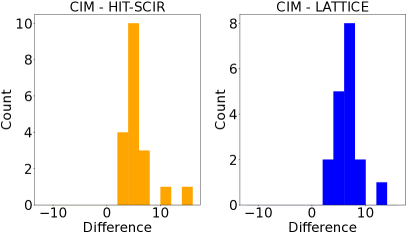
Figure 1: Difference between CIM and ensemble baselines

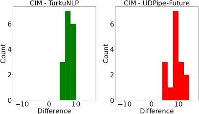
Figure 2: Difference between CIM and non-ensemble baselines

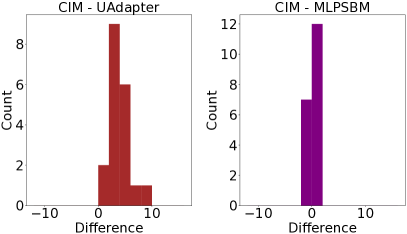
Figure 3: Difference between CIM and LLM-based baselines

Figures 1, 2, and 3 depict the histograms of comparisons between CIM with ensemble, non-ensemble, and LLM-based baselines for high-resource language treebanks. A positive difference means that CIM outperforms. From figure 1, we can observe that CIM outperforms ensemble methods, including HIT-SCIR and LATTICE. From figure 2, we can observe that CIM outperforms non-ensemble methods, including TurkuNLP and UDPipe Future. From figure 3, we can observe that CIM outperforms LLM-based baselines UDapter and MLPSBM. These results support our claim that CIM can correct the mistakes of individual parsers — even the best ones — and outperform them. These results support our claim that CIM is the most suitable DTS aggregation framework among the compared aggregation frameworks in this study.

Table 3: Full results of MST, CRH, CIM compared with the baselines for $19$ high-resource language treebanks. The table is ordered in alphabetical order with respect to the name of the treebank. The columns E1 and E2 refer to ensemble baselines HIT-SCIR Che et al. (2018), and LATTICE Lim et al. (2018), respectively. The columns NE1, NE2 refer to non-ensemble baselines TurkuNLP Kanerva et al. (2018) and UDPipe Future Straka (2018), respectively. The columns L1 and L2 refer to LLM-based parsers UDapter Üstün et al. (2020) and MLPSBM Xu et al. (2022), respectively. The column Avg. refers to the baseline Average.

TB	Sent.	E1	E2	NE1	NE2	L1	L2	Avg.	BEST	MST	CRH	CIM
bg_btb	226	91.4	88.3	89.2	87.1	90.1	95.7	89.6	95.7	92.1	91.0	96.1
ca_ancora	364	91.4	90.0	89.6	90.0	92.6	95.7	83.3	95.7	92.5	91.2	94.6
cs_cac	156	88.5	87.8	88.1	87.3	89.8	95.2	88.8	95.2	90.1	88.9	95.
de_gsd	212	83.6	81.2	81.1	78.3	86.2	89.3	82.2	89.3	83.3	80.2	89.9
en_ewt	340	89.3	88.6	87.1	81.1	90.2	93.4	86.3	93.4	88.6	87.3	93.6
en_gum	199	86.9	90.8	84.1	85.0	91.3	92.8	80.6	92.8	88.4	86.9	93.4
en_lines	286	84.6	85.1	82.6	79.0	87.2	89.4	83.3	89.4	83.3	81.9	90.4
en_pud	264	86.7	88.7	84.0	80.5	88.4	91.3	84.9	91.3	87.2	86.9	92.5
es_ancora	387	89.8	88.7	88.2	88.3	88.9	93.9	88.9	93.9	91.3	89.5	93.6
it_isdt	83	92.7	91.3	90.3	90.9	93.9	96.4	85.1	96.4	93.1	92.6	95.5
it_postwita	136	91.3	21.8	20.5	27.2	92.7	95.2	57.5	95.2	92.6	86.6	95.0
nl_alpino	152	88.6	86.5	85.4	85.6	89.2	92.9	87.2	92.9	89.3	89.5	93.6
nl_lassysmall	116	88.2	86.2	84.5	85.0	89.8	93.9	80.0	93.9	89.7	89.0	94.1
no_bokmaal	466	90.6	88.2	87.7	86.7	91.2	94.5	89.1	94.5	91.3	90.1	94.9
no_nynorsk	378	90.1	87.3	86.4	84.7	91.8	94.6	88.3	94.6	90.9	90.3	95.2
no_nynorsklia	374	70.6	71.7	61.3	62.9	72.4	82.6	64.2	82.6	70.5	72.6	81.3
ro_rrt	199	88.8	87.3	87.7	85.9	89.2	93.2	88.3	93.2	91.7	90.4	94.0
ru_syntagrus	1150	89.9	88.0	88.5	86.0	92.4	95.3	89.3	95.3	92.7	91.8	94.6
ru_taiga	295	77.0	79.7	71.7	72.7	91.9	92.6	70.5	92.6	81.5	80.7	92.8

Table 4: Full results of MST, CRH, CIM compared with the baselines for $52$ low-resource language treebanks. The table is ordered in alphabetical order with respect to the name of the treebank. The columns E1 and E2 refer to ensemble baselines HIT-SCIR Che et al. (2018), and LATTICE Lim et al. (2018), respectively. The columns NE1, NE2 refer to non-ensemble baselines TurkuNLP Kanerva et al. (2018) and UDPipe Future Straka (2018), respectively. The column L1 refers to LLM-based parser UDapter Üstün et al. (2020). The column Avg. refers to the baseline Average.

TB	Sent.	E1	E2	NE1	NE2	L1	Avg.	BEST	MST	CRH	CIM
af_afribooms	158	86.0	86.1	85.9	86.0	87.2	77.4	87.2	87.2	86.3	90.9
ar_padt	55	70.1	70.4	68.8	68.9	85.6	73.3	88.8	90.1	88.4	92.1
br_keb	249	17.4	49.8	48.8	38.5	60.8	43.1	65.6	47.7	64.7	70.2
bxr_bdt	763	35.2	40.4	31.7	32.8	35.8	36.1	46.8	48.4	44.5	51.4
cs_fictree	235	89.3	88.9	88.3	86.5	90.2	87.8	90.2	88.6	89.4	92.2
cs_pdt	1708	90.2	88.5	87.6	85.5	89.4	87.0	90.2	88.3	88.1	91.4
cs_pud	166	88.4	86.4	85.0	85.7	89.1	85.8	89.1	89.2	87.5	91.7
cu_proiel	109	74.2	46.1	44.3	87.9	82.4	61.0	87.9	87.4	85.2	92.6
da_ddt	195	86.4	77.7	77.4	81.5	88.5	81.0	88.5	85.1	83.5	88.9
el_gdt	131	90.1	86.8	88.1	89.2	90.6	87.3	90.7	90.5	90.5	92.4
et_edt	803	85.6	83.7	83.9	81.9	86.3	83.8	86.3	84.8	83.6	88.2
eu_bdt	688	82.9	81.2	81.9	82.0	83.8	81.8	83.8	82.3	81.2	86.2
fa_seraji	204	89.8	88.0	87.6	87.6	89.1	86.3	89.8	88.2	88.4	92.3
fi_ftb	455	85.7	86.1	86.0	80.8	90.4	83.6	90.4	84.9	86.6	90.9
fi_pud	203	87.6	86.1	83.6	81.6	91.3	85.4	91.3	86.8	87.1	91.6
fi_tdt	386	84.9	80.0	78.9	80.6	88.5	81.2	88.5	85.0	85.6	90.2
fo_oft	859	51.3	47.1	37.3	51.6	69.6	53.3	69.6	59.1	67.0	69.4
fr_gsd	89	88.9	88.6	87.9	85.9	90.6	85.1	90.6	89.9	88.6	91.4
fr_sequoia	51	88.9	91.0	87.3	82.7	92.1	78.5	92.1	87.8	88.5	91.7
fro_srcmf	362	79.9	82.9	79.9	82.6	80.3	81.2	82.9	84.0	83.8	87.2
gl_treegal	143	82.8	82.9	82.7	83.2	82.3	82.4	83.2	82.8	83.0	88.7
grc_perseus	544	80.6	74.4	74.2	72.7	82.5	74.9	82.5	75.5	75.8	82.7
grc_proiel	110	81.6	66.6	66.4	61.2	81.7	64.0	81.7	80.3	78.2	86.1
he_htb	55	34.5	32.0	33.0	32.8	88.6	49.4	91.5	91.6	88.1	94.2
hi_hdtb	346	92.0	90.7	91.0	90.1	92.8	91.0	92.8	91.7	90.8	93.5
hr_set	304	88.6	87.5	88.1	83.5	89.4	87.3	89.4	88.7	88.0	91.8

Table 5: Full results of MST, CRH, CIM compared with the baselines for $52$ low-resource language treebanks (Contd.). The table is ordered in alphabetical order with respect to the name of the treebank. The columns E1 and E2 refer to ensemble baselines HIT-SCIR Che et al. (2018), and LATTICE Lim et al. (2018), respectively. The columns NE1, NE2 refer to non-ensemble baselines TurkuNLP Kanerva et al. (2018) and UDPipe Future Straka (2018), respectively. The column L1 refers to LLM-based parser UDapter Üstün et al. (2020). The column Avg. refers to the baseline Average.

TB	Sent.	E1	E2	NE1	NE2	L1	Avg.	BEST	MST	CRH	CIM
hsb_ufal	391	55.0	60.7	44.8	35.7	56.2	44.4	60.7	56.2	64.1	60.8
hu_szeged	212	86.5	77.4	81.3	79.2	85.4	80.2	86.5	82.3	82.2	86.6
kk_ktb	461	42.7	39.9	39.5	38.4	62.3	43.9	62.3	59.5	55.3	65.7
kmr_mg	416	45.1	45.5	40.0	44.5	48.2	41.5	51.6	58.3	54.1	56.2
ko_gsd	255	85.0	84.7	83.8	81.7	86.2	82.9	86.2	84.4	84.3	87.9
ko_kaist	843	86.1	86.1	85.4	85.7	87.3	85.8	87.3	86.7	85.1	89.2
la_ittb	133	85.1	86.0	85.0	83.3	86.2	83.9	86.2	85.5	84.6	87.0
la_perseus	487	77.8	70.1	68.7	65.2	82.4	63.4	82.4	68.4	73.4	83.0
la_proiel	114	86.2	53.2	51.9	78.4	84.8	58.8	86.2	84.2	80.0	84.9
lv_lvtb	414	83.8	77.7	79.7	77.4	81.8	79.1	83.8	81.1	81.1	86.6
pl_lfg	256	89.0	88.3	89.2	89.0	90.6	89.2	90.6	89.8	91.5	93.4
pl_sz	235	88.8	87.2	86.9	86.8	90.1	87.0	90.1	88.4	89.0	91.7
pt_bosque	94	89.9	85.8	84.9	85.5	91.2	82.8	91.2	90.1	87.7	92.4
sk_snk	249	88.3	81.9	82.1	78.0	86.2	82.3	88.3	85.2	87.0	90.4
sl_ssj	181	90.4	69.9	70.1	69.3	82.4	76.9	90.4	89.3	89.0	91.5
sme_giella	507	69.2	70.7	69.9	69.9	71.2	61.6	71.2	71.3	74.4	72.6
sr_set	121	88.3	88.0	87.9	86.2	90.5	87.7	90.5	88.8	90.1	93.2
sv_lines	305	87.2	84.0	83.6	83.2	89.2	76.4	89.2	84.3	83.0	89.5
sv_pud	433	84.6	83.3	83.4	77.4	90.6	82.1	90.6	84.3	85.2	91.3
sv_talbanken	387	88.2	85.0	85.5	82.9	91.6	85.3	91.6	85.9	86.6	91.9
tr_imst	412	75.5	71.8	73.1	72.4	76.7	72.8	76.1	76.1	72.2	80.4
ug_udt	346	82.2	78.7	78.5	78.2	84.3	73.3	82.2	81.3	77.0	82.2
uk_iu	287	90.8	83.9	85.7	83.7	92.8	85.4	90.8	86.3	86.2	88.6
ur_udtb	233	87.7	86.1	85.7	84.6	89.2	86.2	87.7	87.7	85.5	90.9
vi_vtb	87	34.5	37.1	38.2	78.0	82.6	53.8	81.3	81.3	70.3	82.4
zh_gsd	69	83.9	44.0	41.2	41.3	84.7	56.3	86.5	86.5	81.2	88.6

References

- Bininda-Emonds (2004) Olaf RP Bininda-Emonds. 2004. Phylogenetic supertrees: combining information to reveal the tree of life, volume 4. Springer Science & Business Media.
- Bryant (2003) David Bryant. 2003. A classifica of co sensus methods for phylogenetics. In Bioconsensus: DIMACS Working Group Meetings on Bioconsensus: October 25-26, 2000 and October 2-5, 2001, DIMACS Center, volume 61, page 163. American Mathematical Soc.
- Chakraborty et al. (2022) Mohna Chakraborty, Adithya Kulkarni, and Qi Li. 2022. Open-domain aspect-opinion co-mining with double-layer span extraction. In Proceedings of the 28th ACM SIGKDD Conference on Knowledge Discovery and Data Mining, pages 66–75.
- Che et al. (2018) Wanxiang Che, Yijia Liu, Yuxuan Wang, Bo Zheng, and Ting Liu. 2018. Towards better ud parsing: Deep contextualized word embeddings, ensemble, and treebank concatenation. CoNLL 2018, page 55.
- Chen et al. (2021) Mayee Chen, Benjamin Cohen-Wang, Stephen Mussmann, Frederic Sala, and Christopher Ré. 2021. Comparing the value of labeled and unlabeled data in method-of-moments latent variable estimation. In International Conference on Artificial Intelligence and Statistics, pages 3286–3294. PMLR.
- De’Ath (2007) Glenn De’Ath. 2007. Boosted trees for ecological modeling and prediction. Ecology, 88(1):243–251.
- Gavril (1987) Fǎnicǎ Gavril. 1987. Generating the maximum spanning trees of a weighted graph. Journal of Algorithms, 8(4):592–597.
- Kanerva et al. (2018) Jenna Kanerva, Filip Ginter, Niko Miekka, Akseli Leino, and Tapio Salakoski. 2018. Turku neural parser pipeline: An end-to-end system for the conll 2018 shared task. CoNLL 2018, page 133.
- Kuang et al. (2022) Zhaobin Kuang, Chidubem G Arachie, Bangyong Liang, Pradyumna Narayana, Giulia DeSalvo, Michael S Quinn, Bert Huang, Geoffrey Downs, and Yang Yang. 2022. Firebolt: Weak supervision under weaker assumptions. In International Conference on Artificial Intelligence and Statistics, pages 8214–8259. PMLR.
- Kulkarni et al. (2022) Adithya Kulkarni, Nasim Sabetpour, Alexey Markin, Oliver Eulenstein, and Qi Li. 2022. Cptam: Constituency parse tree aggregation method. In Proceedings of the 2022 SIAM International Conference on Data Mining (SDM), pages 630–638. SIAM.
- Kuncoro et al. (2016) Adhiguna Kuncoro, Miguel Ballesteros, Lingpeng Kong, Chris Dyer, and Noah A Smith. 2016. Distilling an ensemble of greedy dependency parsers into one mst parser. In EMNLP.
- Li et al. (2014) Qi Li, Yaliang Li, Jing Gao, Bo Zhao, Wei Fan, and Jiawei Han. 2014. Resolving conflicts in heterogeneous data by truth discovery and source reliability estimation. In Proceedings of the 2014 ACM SIGMOD international conference on Management of data, pages 1187–1198.
- Lim et al. (2018) KyungTae Lim, Cheoneum Park, Changki Lee, and Thierry Poibeau. 2018. Sex bist: A multi-source trainable parser with deep contextualized lexical representations. CoNLL 2018, page 143.
- Mazzetto et al. (2021a) Alessio Mazzetto, Cyrus Cousins, Dylan Sam, Stephen H Bach, and Eli Upfal. 2021a. Adversarial multi class learning under weak supervision with performance guarantees. In International Conference on Machine Learning, pages 7534–7543. PMLR.
- Mazzetto et al. (2021b) Alessio Mazzetto, Dylan Sam, Andrew Park, Eli Upfal, and Stephen Bach. 2021b. Semi-supervised aggregation of dependent weak supervision sources with performance guarantees. In International Conference on Artificial Intelligence and Statistics, pages 3196–3204. PMLR.
- Nivre and McDonald (2008) Joakim Nivre and Ryan McDonald. 2008. Integrating graph-based and transition-based dependency parsers. In Proceedings of ACL-08: HLT, pages 950–958.
- Probst et al. (2019) Philipp Probst, Marvin N Wright, and Anne-Laure Boulesteix. 2019. Hyperparameters and tuning strategies for random forest. Wiley Interdisciplinary Reviews: data mining and knowledge discovery, 9(3):e1301.
- Ratner et al. (2019) Alexander Ratner, Braden Hancock, Jared Dunnmon, Frederic Sala, Shreyash Pandey, and Christopher Ré. 2019. Training complex models with multi-task weak supervision. In Proceedings of the Thirty-Third AAAI Conference on Artificial Intelligence and Thirty-First Innovative Applications of Artificial Intelligence Conference and Ninth AAAI Symposium on Educational Advances in Artificial Intelligence, pages 4763–4771.
- Ratner et al. (2017) Alexander J Ratner, Stephen H Bach, Henry R Ehrenberg, and Chris Ré. 2017. Snorkel: Fast training set generation for information extraction. In Proceedings of the 2017 ACM international conference on management of data, pages 1683–1686.
- Ratner et al. (2016) Alexander J Ratner, Christopher M De Sa, Sen Wu, Daniel Selsam, and Christopher Ré. 2016. Data programming: Creating large training sets, quickly. Advances in neural information processing systems, 29.
- Ravikumar et al. (2010) Pradeep Ravikumar, Martin J Wainwright, and John D Lafferty. 2010. High-dimensional ising model selection using l1-regularized logistic regression. The Annals of Statistics, 38(3):1287–1319.
- Sabetpour et al. (2021) Nasim Sabetpour, Adithya Kulkarni, Sihong Xie, and Qi Li. 2021. Truth discovery in sequence labels from crowds. In 2021 IEEE International Conference on Data Mining (ICDM), pages 539–548. IEEE Computer Society.
- Sagae and Lavie (2006) Kenji Sagae and Alon Lavie. 2006. Parser combination by reparsing. In Proceedings of the Human Language Technology Conference of the NAACL, Companion Volume: Short Papers, pages 129–132.
- Straka (2018) Milan Straka. 2018. Udpipe 2.0 prototype at conll 2018 ud shared task. CoNLL 2018, page 197.
- Surdeanu and Manning (2010) Mihai Surdeanu and Christopher D Manning. 2010. Ensemble models for dependency parsing: cheap and good? In Human Language Technologies: The 2010 Annual Conference of the North American Chapter of the Association for Computational Linguistics, pages 649–652.
- Tian et al. (2021) Yuanhe Tian, Guimin Chen, Yan Song, and Xiang Wan. 2021. Dependency-driven relation extraction with attentive graph convolutional networks. In Proceedings of the 59th Annual Meeting of the Association for Computational Linguistics and the 11th International Joint Conference on Natural Language Processing (Volume 1: Long Papers), pages 4458–4471.
- Üstün et al. (2020) Ahmet Üstün, Arianna Bisazza, Gosse Bouma, and Gertjan van Noord. 2020. UDapter: Language adaptation for truly Universal Dependency parsing. In Proceedings of the 2020 Conference on Empirical Methods in Natural Language Processing (EMNLP), pages 2302–2315, Online. Association for Computational Linguistics.
- Xu et al. (2022) Ziyao Xu, Houfeng Wang, and Bingdong Wang. 2022. Multi-layer pseudo-Siamese biaffine model for dependency parsing. In Proceedings of the 29th International Conference on Computational Linguistics, pages 5476–5487, Gyeongju, Republic of Korea. International Committee on Computational Linguistics.
- Zeman et al. (2018) Daniel Zeman, Jan Hajic, Martin Popel, Martin Potthast, Milan Straka, Filip Ginter, Joakim Nivre, and Slav Petrov. 2018. Conll 2018 shared task: Multilingual parsing from raw text to universal dependencies. In Proceedings of the CoNLL 2018 Shared Task: Multilingual parsing from raw text to universal dependencies, pages 1–21.