Toward Practical Benchmarks of Ising Machines:
A Case Study on the Quadratic Knapsack Problem

Abstract

Combinatorial optimization has wide applications from industry to natural science. Ising machines bring an emerging computing paradigm for efficiently solving a combinatorial optimization problem by searching a ground state of a given Ising model. Current cutting-edge Ising machines achieve fast sampling of near-optimal solutions of the max-cut problem. However, for problems with additional constraint conditions, their advantages have been hardly shown due to difficulties in handling the constraints. The performance of Ising machines on such problems heavily depends on encoding methods of constraints into penalties, but the optimal choice is non-trivial. In this work, we focus on benchmarks of Ising machines on the quadratic knapsack problem (QKP). To bring out their practical performance, we propose to exploit the problem structure upon using Ising machines. Specifically, we apply fast two-stage post-processing to the outputs of Ising machines, which makes handling the constraint easier. Simulation on medium-sized test instances shows that the proposed method substantially improves the solving performance of Ising machines and the improvement is robust to a choice of the encoding methods. We evaluate an Ising machine called Amplify Annealing Engine with the proposed method and found that it achieves comparable results with existing heuristics.

=-21pt

I Introduction

Combinatorial optimization is an important research area with applications in various fields such as artificial intelligence and operations research. For example, the knapsack problem and its variants are famous and well-studied combinatorial optimization problems with numerous applications including production planning, resource allocation, and portfolio selection [1]. Theoretically, combinatorial optimization problems are often hard to solve exactly within a reasonable amount of time due to their NP-hardness. Therefore, various heuristics and meta-heuristics have been developed for dealing with large-scale combinatorial optimization problems.

Ising machines offer a new computing paradigm for tackling hard combinatorial optimization problems [2]. Ising machines search a ground state of a given Ising model, a model in statistical mechanics involving binary variables (called spins) and their interactions, and thus can be used for optimization over binary variables. For problems with additional constraint conditions on binary variables, the penalty method is typically used [3]. Namely, a constraint on binary variables $x=(x_{1},\cdots,x_{n})$ is translated into a penalty term $H_{\mathrm{con}}(x)$ added to the objective function $H_{\mathrm{obj}}(x)$ with a positive coefficient $\lambda>0$ to construct an unconstrained binary optimization problem

$$\operatorname{minimize}\ H_{\mathrm{obj}}(x)+\lambda H_{\mathrm{con}}(x)$$ (1)

$$\operatorname{subject\ to}\ x\in\{0,1\}^{n},$$

to which an Ising machine is applied. There exist several types of Ising machines depending on the way of physical implementation: examples are quantum annealers [4, 5], coherent Ising machines [6, 7], and specialized-circuit-based digital machines [8, 9, 10, 11, 12]. These machines enable fast sampling of near-optimal solutions on the max cut problem, which is naturally formulated with an Ising model.

However, for problems with additional constraint conditions on binary variables, the superiority of Ising machines to other methods has not been observed. For example, previous benchmark results [13, 14, 15, 16] on the quadratic knapsack problem (QKP) and quadratic assignment problem (QAP) show that Ising machines are not competitive with previous (meta-)heuristic solvers. A critical performance issue is that Ising machines do not necessarily output feasible solutions, i.e., solutions satisfying constraints. The penalty coefficient $\lambda$ in (1) is required to be large for outputs to be feasible, but large $\lambda$ typically degrades the objective value. For practical use, it is strongly required to show examples where Ising machines can achieve high performance by overcoming this dilemma and leveraging their strengths.

In this study, we focus on the benchmark of Ising machines on the QKP [17]. The QKP is a well-studied practical problem involving one inequality constraint over binary variables and thus is presumably suitable for solving with Ising machines.

Several methods to encode an inequality constraint into penalties have been proposed and validated [18, 19, 20, 21] to apply Ising machines to the QKP, since the choice of encoding methods has impacts on controlling the trade-off between the feasibility and objective value. Nevertheless, none of them have achieved better results than other heuristic solvers or even a simple greedy method. Moreover, each encoding method has different advantages and disadvantages, making it difficult to select the appropriate method for a given problem instance.

We take another approach to enhance the solving performance of Ising machines by exploiting the problem structure. Specifically, we propose to incorporate efficient two-stage post-processing into the solving process using an Ising machine. The post-processing consists of repair and improvement procedures. First, if the output of the Ising machine is not feasible, the repair procedure is applied to convert it into a feasible solution. The repair procedure resolves the biggest problem of Ising machines that they might output infeasible solutions. This enables us to tune the penalty coefficient according to the objective value, not to the rate of feasible solutions (Fig. 1). Then, the obtained feasible solution is improved by a local improvement procedure. Since Ising machines are suited for global search, the improvement procedure takes a complementary role to achieve further improvement via local search. Both procedures are based on a well-known greedy algorithm that runs sufficiently fast compared to the execution of Ising machines.

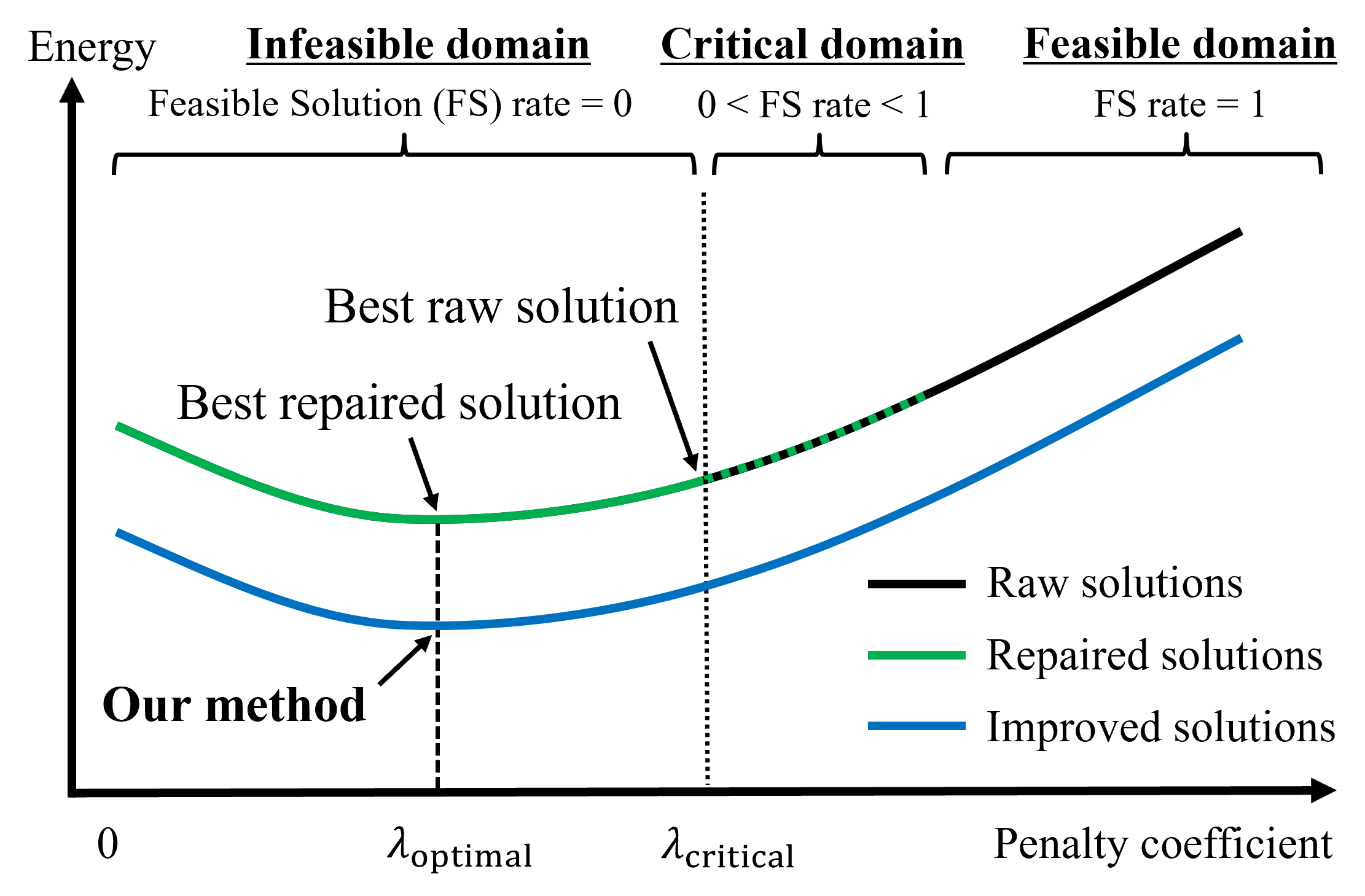
Figure 1: Conceptual figure of effect of proposed method using two-stage post-processing. “Raw solutions” denote outputs of Ising machines, which are often infeasible when penalty coefficient $\lambda$ is small (dashed line on “Critical domain”). Tuning of $\lambda$ typically involves finding $\lambda_{\mathrm{critical}}$ which achieves best trade-off between feasibility and objective. Repair procedure for infeasible solutions enables us to obtain feasible solutions even for smaller $\lambda$. Improvement procedure further enhances feasible solutions with local operations. Optimal penalty coefficient $\lambda_{\mathrm{optimal}}$ is found to be much robust to choice of encoding methods for inequality constraint, in contrast to $\lambda_{\mathrm{critical}}$ which heavily depends on encoding methods (see Section IV).

We conduct simulation experiments on medium-sized QKP instances using simulated annealing. The results show that the combined use of the repair and improvement procedures provides the synergistic effect on gaining the solving performance, achieving optimal solutions on more than 80% of the test instances within a reasonable time. Besides, we find that the post-processing greatly reduces the dependency of the Ising machine performance on the choice of encoding methods of the inequality constraint to penalties, which might make practical use of Ising machines much easier.

Lastly, we evaluate the performance of Amplify Annealing Engine (AE) [22], one of the state-of-the-art Ising machines, with our method on a data set of large QKP instances of size ranging from 1000 to 2000. AE combined with the post-processing achieves best-known solutions on 77.5% of test instances and a small optimality gap on the rest instances. This result significantly exceeds the previous benchmark using Ising machines on QKP and is comparable to the results of previous (meta-)heuristic methods [23, 24, 25, 26].

Our contribution is summarized as follows:

• We propose a method to solve the QKP with Ising machines combined with the post-processing consisting of the repair and improvement procedures.

• Through simulation experiments on medium-sized instances, we show that the post-processing is effective in obtaining optimal solutions and making the performance robust to a choice of encoding methods.

• We benchmark AE, a state-of-the-art Ising machine, on large QKP instances and show that it achieves best-known solutions on 77.5% of them. This is the first result that an Ising-machine-based solver achieves a performance comparable to previous heuristics on the QKP.

The rest of the paper is organized as follows. Backgrounds on Ising machines and the QKP are explained in Section II. We introduce the proposed method in Section III. The simulation experiment is conducted in Section IV. We benchmark the Ising machine in Section V. Related work and future direction is discussed in Section VI. Section VII concludes this paper.

II Ising Machines and Quadratic Knapsack Problem

II-A Ising machines

We briefly review backgrounds on Ising machines. An Ising model is a model in statistical mechanics consisting of a number of binary variables $s_{i}\in\{\pm 1\},i=1,\cdots,n$ called spins and their interactions. The energy of a state $s=(s_{1},\cdots,s_{n})\in\{\pm 1\}^{n}$ is defined as

$$H=\sum_{i,j}J_{ij}s_{i}s_{j}+\sum_{i}h_{i}s_{i},$$ (2)

where $J_{ij}\in\mathbb{R}$ represents the pairwise interaction between spin $s_{i}$ and $s_{j}$ and $h_{i}\in\mathbb{R},i=1,\cdots,n$ is called external field. A ground state of the Ising model is a state $s$ that minimizes the energy $H$. Ising machines implement fast heuristics to search a ground state of the Ising model by analog computation using quantum annealing [27] or degenerate optical parametric oscillators [6], or by digital algorithms such as simulated annealing and simulated bifurcation [12] with massive parallelization.

The problem of finding a ground state of an Ising model can be also formulated as a quadratic unconstrained binary optimization (QUBO) problem [3], which is a class of optimization problems over binary variables $x_{i}\in\{0,1\},i=1,\cdots,n$ defined by a square matrix $Q\in\mathbb{R}^{n\times n}$ as follows:

$$\operatorname{minimize}\ x^{\top}Qx$$ (3)

$$\operatorname{subject\ to}\ x\in\{0,1\}^{n}.$$ (4)

The objective value $x^{\top}Qx$ is also called the energy of $x$.

II-B Quadratic Knapsack Problem

The quadratic knapsack problem (QKP) [17] is a generalization of the well-known knapsack problem and defined by data of $n$ items and the knapsack capacity $C$. Each item $i$ is associated with a weight $w_{i}>0$ and a profit $p_{i}\geq 0$. In addition, for each pair $i,j\ (i<j)$ of items, a pairwise profit $p_{ij}\geq 0$ is defined and it is added to the total profit when both items are put into the knapsack. The QKP asks to maximize the total profit maintaining the total weight within the knapsack capacity. Namely, it is formulated as

$$\operatorname{maximize}\ H(x)\coloneqq\sum_{i=1}^{n}p_{i}x_{i}+\sum_{i=1}^{n-1}\sum_{j=i+1}^{n}p_{ij}x_{i}x_{j}$$

$$\operatorname{subject\ to}\ \sum_{i=1}^{n}w_{i}x_{i}\leq C,$$

$$x_{i}\in\{0,1\},i=1,\cdots,n.$$ (5)

We define $p_{ij}\coloneqq p_{ji}$ for $i>j$ to ease notation. We assume $w_{i}$ and $C$ are integers and satisfy $\min_{i}w_{i}\leq C<\sum_{i=1}^{n}w_{i}$ to avoid triviality. For theory and application of the QKP, we refer to survey papers [28, 1].

As a particular problem structure, it is well-known that an optimum of the QKP is attained on the edge of the space of feasible solutions. Precisely, the following holds. For a proof, we refer to Appendix A.

Proposition 1 (cf. [29]).

For a QKP instance defined as (II-B), an optimum is attained by a solution $x\in\{0,1\}^{n}$ satisfying $C-\max_{i}w_{i}<\sum_{i=1}^{n}w_{i}x_{i}\leq C$.

The QKP can be reformulated as QUBO in the following way [30]. First, an integer slack variable $z\geq 0$ is introduced to represent the inequality constraint $\sum_{i=1}^{n}w_{i}x_{i}\leq C$ as an equality constraint $\sum_{i=1}^{n}w_{i}x_{i}+z=C$. By transforming the equality constraint into a penalty term in the standard way, we get a quadratic optimization problem:

$$\operatorname{minimize}\ -H(x)+\lambda H_{\mathrm{ineq}}(x,z),$$ (6)

$$H_{\mathrm{ineq}}(x,z)=\left(\sum_{i=1}^{n}w_{i}x_{i}+z-C\right)^{2},$$ (7)

where $\lambda>0$ is a sufficiently large positive number. To further translate it into a QUBO problem, the integer variable $z$ is represented by binary variables typically with binary expansion [30]. That is, taking sufficiently large integer $D>0$ which is an upper bound of $z$, $z$ is represented by

$$k \coloneqq\lfloor\log D\rfloor+1,\ R\coloneqq D+1-2^{k-1},$$

$$z =\sum_{i=1}^{k-1}2^{i-1}y_{i}+Ry_{k}$$ (8)

using additional binary variables $y_{1},\cdots,y_{k}\in\{0,1\}$. Other encoding methods of the integer variable is proposed and evaluated for the use of Ising machine (without post-processing) [18, 19, 20]. Their performance will be compared in Section IV under the existence of post-processing.

We remark that a local optimum of the QUBO problem (6) does not necessarily correspond to that of the QKP (II-B). Recall that a local optimum of an optimization problem over binary variables is defined as the objective value of a feasible solution for which any flip (i.e. changing value from 0 to 1 or 1 to 0) of a variable cannot improve the objective value maintaining feasibility. For example, we consider a trivial feasible solution $x=(0,\cdots,0)$ which clearly does not attain a local optimum of the QKP. In the QUBO setting, a solution with $x=(0,\cdots,0)$ and $y$ which gives $z=C$ corresponds to the solution. In fact, it attains a local minimum of the QUBO problem (II-B) for large $\lambda$ since flipping $x_{i}$ for any $i\in\{1,\cdots,n\}$ leads to a change of the objective value by $-p_{i}+\lambda w_{i}^{2}>0$ and similarly flipping $y_{i}$ for any $i\in\{1,\cdots,k\}$ increases the objective value. In other words, a flip of $x_{i}$ in the QKP is realized by multiple flips involving auxiliary variables $y_{i}$ in the QUBO form. Hereafter, unless otherwise noted, we use the word “local” in the sense of the QKP and not of QUBO.

II-C Challenges in Ising Machines Solving QKP

Since the QKP can be naturally formulated with a quadratic objective function of binary variables as above, it is presumably suited for benchmarks of Ising machines. However, in contrast to the max-cut problem on which Ising machines have achieved successful results [7, 12], even medium-sized QKP instances that can be handled by exact methods are not adequately optimally solved by Ising machines or simulation in the previous studies [15, 19, 20]. The biggest challenge is that Ising machines might output solutions violating the inequality constraint since the constraint is imposed only implicitly with the penalty term.

There is a trade-off that a large penalty is required to obtain feasible solutions with high probability whereas it also degrades the objective value. As shown in Section IV below, the recently proposed encoding methods of the inequality constraint [18, 19, 20] have a role to control this trade-off. Nevertheless, their improvement in Ising machine performance is not satisfactory, since they are still outperformed by a simple greedy method (see simulation results in Section IV). Our approach is to directly resolve the trade-off by incorporating local post-processing into Ising machines, instead of exploring the optimal encoding method.

III Proposed Method

We propose to incorporate post-processing utilizing the problem structure into the solving process with Ising machines. The post-processing consists of two steps: repair and improvement. The repair procedure converts an infeasible solution into a feasible solution. It is commonly used for other meta-heuristics such as evolutionary algorithms [25, 31]. The improvement procedure takes a feasible solution as an input and improves the objective value by locally modifying the solution. Both procedures are building blocks of most heuristic combinatorial optimization algorithms, often combined with randomized operations to enable global search [26, 32]. In our case, they are used deterministically (i.e., without randomness) following a greedy strategy, since Ising machines have a role in the global search. We expect that Ising machines and the local post-processing work complementarily to efficiently enhance the solving performance. One important advantage of the proposed method is that the repair procedure enables us to set the penalty coefficient $\lambda$ in (6) to small values and to tune $\lambda$ according to the objective value, not to the rate of feasible solutions, since obtained solutions are always feasible. This effect, coupled with the local improvement, helps us to obtain the optimal solution more easily with Ising machines, as we will see in Sections IV and V. We explain the details of the method below.

III-A Post-processing Algorithm on QKP

Algorithm 1 Post-processing on QKP

1:Solution $x=(x_{1},\cdots,x_{n})\in\{0,1\}^{n}$ (possibly infeasible), Profits $(p_{i})_{i},(p_{ij})_{ij}$, Weights $(w_{i})_{i}$, Capacity $C$

2:Feasible solution $x$

3:for $i=1,\cdots,n$ do

4:    $e_{i}\leftarrow(p_{i}+\sum_{j=1}^{i-1}p_{ji}x_{j}+\sum_{j=i+1}^{n}p_{ij}x_{j})/w_{i}$

5:while $\sum_{k}w_{k}x_{k}>C$ do

6:    Take $j\in{\operatorname{argmin}}\{e_{i}\mid x_{i}=1\}$

7:    $x_{j}\leftarrow 0$ $\triangleright$ Remove an item

8:    Update $(e_{i})_{i}$

9:for $j$ s.t. $x_{j}=0$ in decreasing order of $e_{j}$ do

10:    if $\sum_{k}w_{k}x_{k}+w_{j}\leq C$ then

11:         $x_{j}\leftarrow 1$ $\triangleright$ Add an item

12:         Update $(e_{i})_{i}$     

13:for $i$ s.t. $x_{i}=1$ in increasing order of $e_{i}$ do

14:    for $j$ s.t. $x_{j}=0$ in decreasing order of $e_{j}$ do

15:         if $\sum_{k}w_{k}x_{k}-w_{i}+w_{j}\leq C$ and $e_{i}w_{i}<e_{j}w_{j}-p_{ij}$ then

16:             $x_{i}\leftarrow 0$, $x_{j}\leftarrow 1$ $\triangleright$ Swap items

17:             Update $(e_{i})_{i}$              

18:return $x$

Both the repair and improvement procedures are built upon well-known greedy heuristics used in the previous studies [17, 33, 29]. We review the ideas of both procedures briefly to make the argument self-contained.

For the repair procedure, we note that an infeasible solution can be made into a feasible solution by removing several items from the knapsack since the weights are positive and there is a trivial feasible solution $x=(0,\cdots,0)$. To reduce the loss of the objective value, items to be removed are selected one by one greedily. On the simple knapsack problem with the linear objective, a greedy strategy is typically based on a metric called efficiency defined by a ratio of the profit and weight of the item. In the QKP, the efficiency $e_{i}(x)$ of item $i$ with respect to an incumbent solution $x$ is defined as

$$e_{i}(x)\coloneqq\frac{p_{i}+\sum_{j=1}^{i-1}p_{ji}x_{j}+\sum_{j=i+1}^{n}p_{ij}x_{j}}{w_{i}}.$$ (9)

Consequently, item $i$ with $x_{i}=1$ achieving minimum $e_{i}(x)$ is removed iteratively until the constraint is satisfied. Note that this greedy removal operation is previously used for a constructive heuristic with an input $x=(1,\cdots,1)$ [33, 29].

The improvement procedure consists of so-called fill-up and exchange (FE) operation [17], which is widely used in heuristic methods on the QKP [23, 25]. The fill-up operation puts items into the knapsack unless it violates the capacity constraint. Then, the exchange operation replaces an item in the knapsack with another item that is not in the knapsack, so that it improves the objective value maintaining feasibility. In other words, the fill-up operation modifies a feasible solution to a local optimum, and the exchange operation searches neighborhood local optima. In our method, the order of item selection for FE operation is again based on the greedy strategy with the efficiency $e_{i}(x)$. An item to be included in the knapsack is chosen following the descending order of $e_{i}(x)$ and an item to be removed from the knapsack is chosen following the ascending order of $e_{i}(x)$.

The overall process is summarized in Algorithm 1. Every time the solution $x$ is changed, the efficiency $e_{i}$ is updated with computational cost of order $O(n)$. The total complexity of the algorithm is $O(n^{3})$ in the worst case, but the number of the exchange operation (which is the bottleneck) is typically much less than $n^{2}$, and so the algorithm runs practically fast.

The post-processing above is closely related to a greedy heuristic proposed by Billionnet and Calmels [29]. Their method is to first obtain a feasible solution with the greedy removal operation for $x=(1,\cdots,1)$ and then apply the FE operation. In particular, when the penalty coefficient $\lambda$ in (6) is set to $0$, then the optimal solution is obviously $x=(1,\cdots,1)$. Thus, for sufficiently small $\lambda$, an Ising machine with the post-processing outputs the same solution as the one obtained by the greedy method.

The ideas of the repair and improvement procedures are not new as mentioned above. Besides, more elaboration on the post-processing possibly improves the solving performance further with additional computational costs. In this study, the specific implementation is not of much interest. Rather, we aim to show that combining simple operations based on well-known ideas to form post-processing effectively overcomes the critical performance issue of Ising machines.

(a) $n=100$

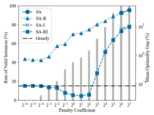
(b) $n=200$

(c) $n=300$

Figure 2: Optimality gap (line graph) and number of instances on which feasible solutions are obtained with SA (bar chart) for each problem size $n$ of QKP instances. Optimality gap for SA and SA-I is plotted only for $\lambda$ producing feasible solutions on all instances. By combining repair and improvement procedures, SA-RI achieves smaller optimality gap than greedy method.

IV Simulation Experiments

We validate the proposed method via simulation of Ising machines on the basis of simulated annealing (SA) that takes a QUBO problem as an input. Note that most digital Ising machines are based on SA [8, 9], and also SA is treated as a classical counterpart of quantum annealing [34, 35]. Therefore, controlled experiments with SA provide informative insights on the use of Ising machines. For a test bed, we use a data set of 100 medium-sized QKP instances generated in the previous study [36]. There are 10 generated instances for each combination of the problem size $n\in\{100,200,300\}$ and density $d\%$ of the objective function for $d\in\{25,50,75,100\}$ except for $(n,d)=(300,75)$ and $(300,100)$. Specifically, the pairwise profit $p_{ij}\ (i<j)$ is non-zero with probability $d/100$ in the generation procedure. The exact optimal solutions of these instances are known and the data set has been used in the existing benchmark of Ising machines [15, 19, 20]. Things to be verified are as follows: (i) better solutions (in particular, the optimal solutions) are obtained by utilizing the post-processing and (ii) the computational cost for the post-processing is sufficiently small compared to the rest of the whole process. Furthermore, we re-evaluate various encoding methods of the inequality constraints [18, 19, 20] under the existence of the post-processing to verify the robustness of the proposed method.

IV-A Computational Set-up

Each QKP instance is translated into a QUBO problem (6) with binary encoding (II-B) of the integer variable $z$ where the upper bound $D$ of $z$ is set to the capacity $C$. The penalty coefficient $\lambda$ is varied for $\lambda=2^{i},i=-6,-5,\cdots,6,7$. For each $\lambda$, SA is executed 10 times to obtain 10 solutions. The setting of SA is as follows. We use the public implementation of SA on D-Wave Ocean SDK of version 6.4.1. In the algorithm, the temperature is successively decreased from the initial value to the end value, iterating an inner loop consisting of Monte-Carlo (MC) steps for all variables. Following the previous studies [18, 19], the number of inner loops is set to $10^{6}$ and the initial and end temperatures are set to $n\max_{i,j}|Q_{i,j}|$ and $0.1$, respectively. Here, $Q_{i,j}$ is the QUBO matrix for (6), i.e.,

$$\sum_{i,j:i\leq j}Q_{i,j}\hat{x}_{i}\hat{x}_{j}=-H(x)+\lambda H_{\mathrm{ineq}}(x,z),$$ (10)

where $\hat{x}=(x_{1},\cdots,x_{n},y_{1},\cdots,y_{k})$ is a vector of the whole variables including $y_{1},\cdots,y_{k}$ in (II-B). The experiment program is coded with python 3.11.4 and run on a CentOS (version 7.6.1810) server with Intel Xeon Gold 6130 chip.

We set SA without post-processing (which we simply call SA) and the greedy algorithm described in Section III as baselines, and compare them to SA with the repair and/or improvement procedure (which we call SA-R, SA-I, and SA-RI, respectively). We summarize the compared methods in Table I. The quality of a solution is evaluated via the optimality gap

$$\mathrm{Optimality\ Gap}={\frac{S_{\mathrm{best}}-S}{S_{\mathrm{best}}}}\times 100\ (\%),$$ (11)

where $S_{\mathrm{best}}$ is the optimal value for the QKP instance and $S$ is the objective value of the solution. For methods other than the (deterministic) greedy method, the optimality gap is taken as the minimum over all feasible solutions obtained for each $\lambda$. For SA, we also count the number of instances on which a feasible solution is obtained, for each $\lambda$. The optimality gap for SA and SA-I is reported only for instances on which they obtain at least one feasible solution.

TABLE I: Description of Compared Methods.

Name	Description
Greedy	Equivalent to post-processing on $x=(1,\cdots,1)$
SA	SA without post-processing (may output infeasible solutions)
SA-R	SA with repair procedure
SA-I	SA with improvement procedure (only for feasible solutions)
SA-RI	SA with both repair and improvement procedures

IV-B Results

IV-B1 Observations from Tuning of Penalty Coefficients

The optimality gap of each method aligned with the penalty coefficient $\lambda$ averaged over instances of the same size are shown in Fig. 2. We also show the rate of the number of instances where SA outputs at least one feasible solution (which we call valid instances) as bar charts. For SA and SA-I, the optimality gap is plotted only when feasible solutions are obtained on all instances for each $\lambda$ and not shown otherwise. The first thing to observe from the results of SA is that the rate of valid instances increases for large $\lambda$, whereas large $\lambda$ degrades the optimality gap. Therefore, SA achieves its smallest optimality gap on the minimum $\lambda_{\mathrm{SA}}$ among those giving feasible solutions on all instances, i.e., $\lambda_{\mathrm{SA}}=32$ for $n=100$ and $\lambda_{\mathrm{SA}}=64$ otherwise. Note that the best optimality gap of SA is much worse than that of the greedy method. Since the greedy method runs several orders of magnitude faster than SA, we conclude that SA without post-processing is completely inferior to the greedy method on the QKP. When the repair method is applied, the optimality gap of SA-R roughly extrapolates that of SA, as expected. Accordingly, the optimality gap of SA-R achieves smaller values than that of SA for $\lambda<\lambda_{\mathrm{SA}}$. This result indicates the effectiveness of tuning $\lambda$ based on the objective value instead of the rate of feasible solutions, which is realized thanks to the repair procedure. A similar phenomenon has been observed by Fukada et al. [37] on a variant of the QAP. The optimality gap is further reduced after combining with the improvement procedure. Although using only either of the two procedures is not sufficient to outperform the greedy method, SA-RI using both procedures achieves a smaller optimality gap than that of the greedy method. This suggests that the two procedures might successfully improve the solving performance of Ising machines synergistically. Note that as $\lambda$ gets closer to 0, the optimality gap of SA-RI converges to that of the greedy method. This is expected as we argued in Section III, that is, SA outputs the trivial solution $x=(1,\cdots,1)$ for extremely small $\lambda$. The same argument applies to SA-R; as $\lambda\to 0$, the optimality gap converges to that of a weak version of the greedy algorithm that only repairs $x=(1,\cdots,1)$.

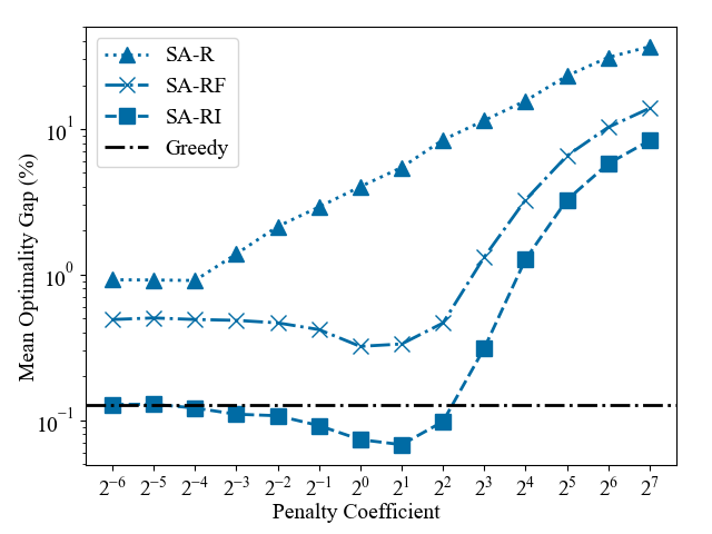
Figure 3: Optimality gap averaged over 100 medium-sized instances. SA-RF denotes SA-R followed by fill-up operation, which produces locally optimal solutions. Fill-up operation improves solutions of SA-R particularly around $\lambda=2$, which is optimal penalty coefficient for SA-RI.

There are two other interesting observations from Fig. 2 regarding the optimal penalty coefficient $\lambda$. One is that $\lambda$ minimizing the averaged optimality gap of SA-RI seems independent of the problem size $n$. We discuss this phenomenon in Section IV-D, where the dependence of the optimal $\lambda$ on instance data including $n$ and other factors is analyzed quantitatively. The other observation is that $\lambda$ minimizing the optimality gap of SA-R and that of SA-RI completely differ: $\lambda_{\text{SA-R}}$ for SA-R is near 0 and $\lambda_{\text{SA-RI}}$ for SA-RI is around 2 for all problem size $n$. The result leads to apparently strange inconsistency that the outputs of SA-R around $\lambda=2$ can be improved to good solutions, but themselves are far from optimal. We hypothesized that this is because SA-R outputs solutions distant from local optima particularly when $\lambda$ is around 2. To see this, we plot the optimality gap for SA-R followed by only the fill-up operation, which we call SA-RF, in Fig. 3. Here, we show the results averaged over all 100 instances due to the space limit and similarity of the results, and refer to Appendix B-A for the results on each problem size $n$. The optimality gap of SA-RF attains its minimum around $\lambda=1$, which is similar to SA-RI, and the difference between SA-R and SA-RF is significantly large there. Since the fill-up operation makes a solution locally optimal, the result implies that the solutions obtained with SA-R are far from local optima around $\lambda=2$. This finding contains an important suggestion on the use of Ising machines: by carefully tuning the penalty coefficient, we can obtain a solution that is itself not good but globally (i.e., up to greedy local operations) near-optimal. We also note that the gap between SA-R and SA-RF cannot be easily filled by emphasizing the local search phase in SA, e.g., by lowering the end temperature. This is because the local operations on the QUBO problem do not correspond to those on the QKP, as described in Section II.

TABLE II: Number of Medium-sized Instances Optimally Solved.

$n\_d$	Greedy	SA	SA-R	SA-I	SA-RI
100_25	3	0	3	6	9
100_50	4	1	1	8	10
100_75	4	1	4	6	9
100_100	4	0	2	8	10
200_25	2	0	0	5	9
200_50	4	0	2	3	6
200_75	4	0	1	3	8
200_100	2	0	1	5	5
300_25	4	0	2	3	8
300_50	4	0	1	5	8
Total	35	2	17	52	82

TABLE III: Average Optimality Gap (%).

$n\_d$	Greedy	SA	SA-R	SA-I	SA-RI
100_25	0.370	6.651	0.797	0.139	0.047
100_50	0.101	6.358	0.272	0.103	0.000
100_75	0.115	5.821	0.208	0.426	8.4E-3
100_100	0.196	10.202	0.395	7.0E-3	0.000
200_25	0.173	9.404	0.325	0.318	5.1E-3
200_50	0.049	8.624	0.122	0.421	0.011
200_75	0.049	8.624	0.200	2.259	2.9E-3
200_100	0.062	10.357	0.206	0.995	0.034
300_25	0.127	10.098	0.230	0.484	1.4E-3
300_50	0.038	11.329	0.245	1.415	4.4E-4
Mean	0.128	8.747	0.300	0.657	0.011

IV-B2 Results on Best Optimality Gap

The number of instances on which each method achieved the optimal solution is reported in Table II. We also summarize the optimality gap averaged over 10 instances for each pair $(n,d)$ in Table III. SA achieves the optimal solutions on only two instances among 100 instances in total. Although SA-R achieves the optimum on several instances, the total number of such instances is less than that of the greedy method. SA-I obtains the optimal solutions more frequently than SA-R and the greedy method, but its averaged optimality gap is worse than the others. This means that the quality of solutions of SA-I has much variance over instances, which is often undesirable. SA-RI, the proposed method, successfully attains the optimum on 82 instances in total and achieves the smallest optimality gap for all pairs of $(n,d)$. These results clearly demonstrate the effectiveness of combining the repair and improvement procedures as the post-processing for SA. For full results on each instance, see Appendix B-A.

TABLE IV: Average Processing Time.

	Before Post-process (s)		Post-process (ms)
$n\_d$	Formulation	SA	Repair	Improve
100_25	0.07	4.4	0.9	1.0
100_50	0.07	4.3	1.0	1.0
100_75	0.07	4.0	1.0	0.9
100_100	0.07	3.7	1.0	0.8
200_25	0.23	17.3	3.5	3.7
200_50	0.24	17.0	3.8	3.7
200_75	0.24	14.0	4.1	2.9
200_100	0.25	12.8	3.9	2.8
300_25	0.51	34.4	8.1	7.0
300_50	0.52	36.5	8.8	7.0

IV-B3 Results on Processing Time

We evaluate the overhead of the post-processing. The average processing time for each process is reported in Table IV. In addition to the execution time of SA and the repair and improvement procedures, we include the processing time to create the input QUBO object after reading data of the corresponding QKP instance in the “Formulation” column. Note that we report processing time before the post-processing in seconds and time for the post-processing in milliseconds. The time required for the post-processing is more than 1000 times less than that of the annealing, and also much less than the formulation. We also see that time for each process increases roughly with an order of $n^{2}$. Although the execution time of a real Ising machine might scale with a smaller order, the post-processing should still have a sufficiently small overhead, as it is shorter than the time for formulation. Therefore, the proposed method improves the performance with a negligibly small amount of additional computational cost.

IV-C Dependency on Encoding Methods

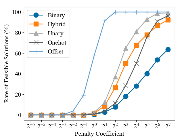
(a) Rate of Feasible Solutions

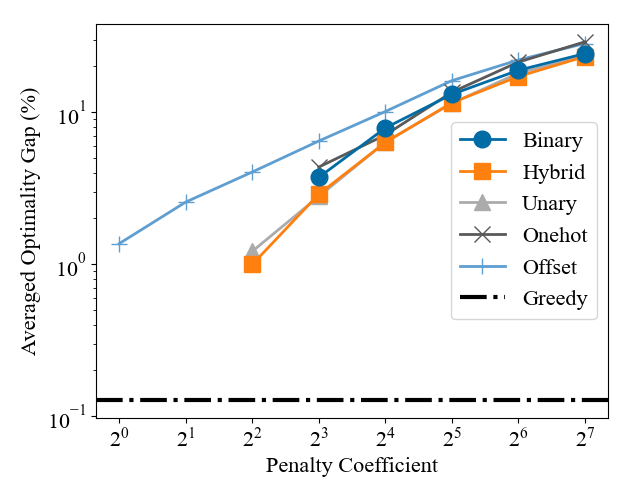
(b) Optimality Gap of SA

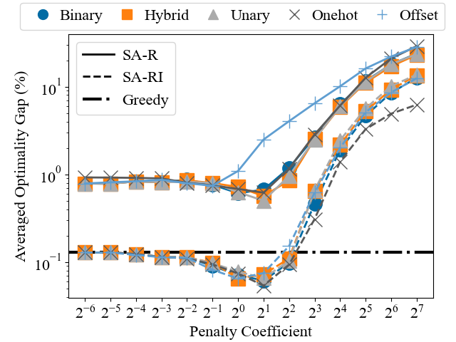
(c) Optimality Gap with Post-processing

Figure 4: Performance comparison among various encoding methods of inequality constraint on 100 medium-sized QKP instances. (a)(b) Choice of encoding methods controls trade-off between rates of feasible solutions and objective values. (c) Solving performance of proposed method is much less dependent on choice of encoding methods.

As described in Section II, the previous studies [18, 19, 20] suggest that other encoding methods of the slack variable $z$ in (6) than the standard binary encoding (II-B) might enhance the quality of solutions obtained by Ising machines. Since their evaluation has been conducted without any post-processing, we re-evaluate various encoding methods with the proposed post-processing in this section.

The setting is as follows. We consider the following five variations of encoding methods of $z$ in the QUBO problem (6) of the QKP. The first is the binary encoding shown in (II-B). Recall that it involves $k$ auxiliary variables $y_{1},\cdots,y_{k}$ with $k=\lfloor\log D\rfloor+1$, where $D$ denotes the upper bound of $z$. The second is the unary encoding defined as

$$z=\sum_{i=1}^{D}y_{i},$$ (12)

which involves $D$ auxiliary variables $y_{1},\cdots,y_{D}$. The third is the hybrid encoding [19], which hybridizes the unary and binary encoding. As it has several degrees of freedom, we adopt the following form close to a method called $HE(1)$ in the previous experiment [19]:

$$z=\sum_{i=1}^{k}y_{i}+\sum_{i=k+1}^{2k}2y_{i},\ k\coloneqq\lceil D/3\rceil.$$ (13)

The hybrid encoding involves $2\lceil D/3\rceil$ auxiliary variables. The fourth is the one-hot encoding, which uses an additional penalty term $H_{\mathrm{onehot}}$ and modify the objective function of the QUBO problem as

$$-H(x)+\lambda\left(H_{\mathrm{ineq}}(x,z)+H_{\mathrm{onehot}}\right),$$ (14)

defining

$$z=\sum_{i=0}^{D}iy_{i},\ H_{\mathrm{onehot}}=\left(\sum_{i=0}^{D}y_{i}-1\right)^{2}.$$ (15)

The one-hot encoding involves $D+1$ auxiliary variables. The last is the offset encoding [20], which set $z$ to a constant

$$z=W_{\mathrm{offset}}$$ (16)

with some small number $W_{\mathrm{offset}}\geq 0$. Since $z$ does not work as a slack variable any more, the offset encoding does not preserve the equivalence of the optimization problems. Nevertheless, Bontekoe et al. [20] reported that it outperformed other encoding methods. We set $W_{\mathrm{offset}}=3$ following the previous result. All methods other than the offset encoding involve the upper bound $D$ of $z$. Note that it suffices to set $D$ to a value greater than or equal to $\max_{i}w_{i}$ to translate the QKP to the QUBO problem preserving the optimum according to Proposition 1. On the other hand, since methods other than the binary encoding uses $O(D)$ auxiliary variables, $D$ should be sufficiently small to effectively apply Ising machines. Therefore, we set $D$ to $\max_{i}w_{i}$ in this experiment. Other settings are identical to those in the earlier experiment.

We remark that an output of Ising machines or SA can have a positive penalty $H_{\mathrm{ineq}}(x,z)>0$ (or $H_{\mathrm{onehot}}>0$ for the one-hot encoding) even if the solution $x$ is feasible. Such situations include a case where $z\neq\sum_{i}w_{i}x_{i}$, as well as a case where $\sum_{i=0}^{D}y_{i}\neq 1$ for the one-hot encoding. It is in contrast to the previous evaluation [18] treating the solution as feasible only when it has zero penalty, and this difference in definition could lead to different results. In particular, for the one-hot encoding above, it is actually not necessary to impose the one-hot constraint $\sum_{i=0}^{D}y_{i}=1$, since the inequality constraint can be satisfied even when $\sum_{i=0}^{D}y_{i}=0$ or $\sum_{i=0}^{D}y_{i}\geq 2$. Note that this fact is also used in the previous study [20]. Therefore, the aforementioned case where $x$ is feasible and $H_{\mathrm{onehot}}>0$ can particularly often occur, and we indeed observed this phenomenon in our experiment.

Fig. 4 shows the results over various $\lambda$. Fig. 4a shows the rate of feasible solutions (we call FS rate) over all instances for each encoding. On all methods, a larger penalty coefficient results in a high FS rate. Among the tested encoding methods, the binary encoding leads to the lowest, while the offset encoding achieves the highest. The difference might be explained by the number of flips of auxiliary variables $y_{i}$ required for a flip of a variable $x_{i}$, which is mentioned in Section II. More precisely, multiple MC steps in SA are required to realize a single flip on the QKP. The offset encoding uses no auxiliary variables, and thus the penalty $H_{\mathrm{ineq}}$ might be easily decreased by local operations in SA, leading to the high FS rate. In contrast, a lot of MC steps are required for changing the value of $z$ for the binary encoding, resulting in a low FS rate. The redundancy of the representation (i.e. representing a value of $z$ by multiple combinations of values of $y_{1},y_{2},\cdots$) in the unary and hybrid encoding might help to make the number of required MC steps small [18], and thus they give the intermediate results. For the one-hot encoding, most solutions violate the one-hot constraint and as a result obtain a similar redundancy, which again explains the intermediate result. The optimality gap of the feasible solutions obtained by SA is shown in Fig. 4b. Here, we plot the optimality gap for $\lambda$ that obtains a feasible solution on more than half of all instances to exclude outlier values. Again, for all methods, a smaller penalty coefficient leads to better objective values. The hybrid, unary, and offset encodings achieve a lower optimality gap than the others, due to the high FS rate at small $\lambda$. These results on the FS rate and optimality gap mostly agree with the previous studies [18, 19, 20].

Fig. 4c shows the optimality gap for each method combined with the post-processing. Interestingly, after the post-processing, the difference among the encoding methods gets almost negligible and all methods reach a similar minimum optimality gap at the similar value of $\lambda$. A subtle exception is the offset encoding; SA-R with the offset encoding attains the minimum optimality gap at $\lambda_{\text{SA-R}}=0.5$, unlike the others. This is presumably because fixing the slack variable $z$ to a constant changes the effect of penalty $H_{\mathrm{ineq}}$ on the behavior of SA. The overall result indicates that the proposed method is much robust to the choice of encoding methods, compared to SA without post-processing. A fundamental reason for the somewhat surprising similarity of the post-processed outputs over the various encoding methods is unclear and might be related to the behavior of the SA algorithm. Since a precise algorithmic analysis is beyond the scope of this paper, further investigation is left as future work.

TABLE V: Number of Medium-sized Instances Optimally Solved.

$n\_d$	Binary	Hybrid	Unary	One-hot	Offset
100_25	10	9	8	10	10
100_50	9	9	9	9	9
100_75	9	8	8	8	8
100_100	8	8	8	9	7
200_25	9	8	10	8	8
200_50	7	7	6	7	7
200_75	8	9	9	8	8
200_100	6	6	6	6	6
300_25	7	7	7	8	8
300_50	10	9	9	8	9
Total	83	80	80	81	80

TABLE VI: Averaged Optimality Gap ($\times 0.01$ %).

$n\_d$	Binary	Hybrid	Unary	One-hot	Offset
100_25	0.000	9.328	4.355	0.000	0.000
100_50	0.384	0.610	0.610	0.666	0.610
100_75	0.537	1.590	1.590	1.140	1.140
100_100	0.412	0.412	14.338	0.205	14.546
200_25	0.510	0.659	0.000	0.253	3.585
200_50	0.343	0.888	0.761	0.260	0.888
200_75	0.917	0.213	0.213	0.297	0.884
200_100	0.995	1.079	1.129	0.624	0.803
300_25	0.418	3.710	0.180	0.135	0.246
300_50	0.000	0.035	0.241	0.055	0.184
Mean	0.452	1.853	2.342	0.363	2.288

For a quantitative performance comparison, we summarize the number of instances optimally solved and the optimality gap for each encoding with the proposed method in Table V and VI. We see that the binary and one-hot encodings slightly outperform the other methods on average in terms of both metrics. In particular, among the binary, unary, and one-hot encodings, the unary encoding performs the worst (by a possibly negligible margin), in contrast to the previous evaluation without the post-processing [18]. In other words, whether or not a specific encoding method performs well can be easily changed by additional operations. This leads to an insight important to practitioners that performance evaluation of Ising machines must be carefully done in a practical situation involving several pre- or post-processing of the problem or solutions.

IV-D Analysis of Optimal Penalty Coefficients

In the earlier experiments, we observed that the optimal penalty coefficient $\lambda_{\text{SA-RI}}$ for the proposed method varies depending on the problem instances (see Appendix B-A for full results including $\lambda_{\text{SA-RI}}$ for each instance). The optimal penalty coefficient could be estimated by some representative features of the instance data [37]. In this section, we analyze $\lambda_{\text{SA-RI}}$ over the tested instances to utilize the result for solving larger instances in the later section.

As representative features of the QKP, we consider the problem size $n$, density $d$ of the objective function, and tightness ratio $\alpha=C/\sum_{i}w_{i}$ of the inequality constraint. Note that the tightness ratio $\alpha$ has not been mentioned in the QKP literature, whereas it is recognized as an important factor in the context of the multi-dimensional knapsack problem [31, 38]. We expect that $n$ has weak correlation with $\lambda_{\text{SA-RI}}$, as we see from Fig. 2 for each $n$. On the other hand, the density $d$ involves the scale of the increase in the objective value for putting an item into the knapsack. Since it is typically considered that the scales of the objective function and penalty should be balanced when applying the penalty method, we expect that $\lambda_{\text{SA-RI}}$ tends to be large for large $d$.

TABLE VII: Coefficients for Optimal Penalty Coefficients.

$A$	$c_{n}$	$c_{d}$	$c_{\alpha}$
$1.14$	$0.09$	$0.84$	$-0.21$

We model $\lambda_{\text{SA-RI}}$ as the product of the features by

$$\lambda_{\mathrm{Estimate}}=An^{c_{n}}d^{c_{d}}\alpha^{c_{\alpha}},$$ (17)

where $A,c_{n},c_{d},$ and $c_{\alpha}$ are parameters to be fit. We show the results of log-linear regression on $\lambda_{\text{SA-RI}}$ for the tested 100 instances in Table VII. As expected, the resulting coefficient for $n$ is close to 0 and that for $d$ is a large positive value. The coefficient $c_{\alpha}$ for $\alpha$ is negative, which means that $\lambda$ should be lowered for large capacity $C$. This might be because large $\alpha$ implies that feasible solutions occupy a large fraction of the total space $\{0,1\}^{n}$, and thus the penalty is not required to be much emphasized for solving the QKP. Note that the overall analysis is on a data set created following a specific procedure of instance generation, and the result might depend on the distribution of problem instances. Since larger instances used in the later section are based on the same generating protocol as that of the instances used above, we make use of the analysis result to solve the larger instances.

V Benchmark of Ising Machine

In this section, we benchmark one of the state-of-the-art Ising machines, Amplify Annealing Engine (AE) [22], on a broader set of QKP instances. Our aim in this experiment is to verify that the proposed method works also for a high-performance Ising machine as well as for naive SA. We evaluate AE with the post-processing on large QKP instances which cannot be handled with exact methods, and compare its performance with existing heuristic solvers.

V-A Setting

In addition to the medium-sized instances in Section IV, we use another group of QKP instances generated in the previous study [24]. There are 10 instances for each combination of the problem size $n\in\{1000,2000\}$ and density $d\in\{25,50,75,100\}$ of the objective function in the data set. Their exact optimal solutions have not been known and the current best-known objective values are reported by Chen and Hao [26]. Therefore, we use their result to compute the optimality gap (11) in which $S_{\mathrm{best}}$ denotes the best-known objective value.

The computational environment is the same as in Section IV. We provide additional details on the use of the Ising machine. We use AE of version 0.7.4 with A100 GPU. The timeout for the execution of AE is set to $0.01n$ seconds for problem size $n$, which is comparable with that of the existing solver [26]. We use Amplify SDK [22] of version 0.11.2 to translate the QKP into a QUBO problem and input it to AE. The slack variable $z$ is encoded into binary variables by binary expansion (II-B) with $D=C$.

The penalty coefficient $\lambda$ is heuristically varied as

$$\lambda=a\frac{d}{100}\sqrt{1/\alpha},\ a=1,2,\cdots,$$ (18)

using the density $d$ and tightness ratio $\alpha=C/\sum_{i}w_{i}$, based on the result in Section IV-D. The upper bound of $a$ is set to 10 for medium-sized instances and 20 for large instances, which is found to be sufficient to obtain good solutions with the proposed method. The Ising machine is executed 10 times to sample 10 solutions for each $\lambda$. The solutions are evaluated by optimality gap with and without the post-processing.

TABLE VIII: Number of Medium-sized Instances Optimally Solved.

$n\_d$	Gurobi	AE	AE-R	AE-I	AE-RI
100_25	10	10	10	10	10
100_50	10	10	10	10	10
100_75	10	10	10	10	10
100_100	10	10	10	10	10
200_25	10	7	8	10	10
200_50	9	8	8	10	10
200_75	10	7	8	10	10
200_100	10	7	7	10	10
300_25	10	5	7	10	10
300_50	10	6	8	10	10
Total	99	80	86	100	100

We compare the performance of AE with and without the post-processing. We call them AE, AE-R, AE-I, and AE-RI, respectively, following the same notation in Table I. We use the greedy method described in Section III as a baseline. Besides, the results of the following heuristic solvers tailored for the QKP are taken from the existing papers [25, 26] and included as baselines: dynamic programming with fill-up and exchange (DP+FE) [23], GRASP combined with tabu search (GRASP+Tabu) [24], improved quantum-inspired evolutionary algorithm (IQIEA) [25], and iterated hyper-plane exploration approach (IHEA) [26]. We also use Gurobi [39], one of the state-of-the-art commercial solvers, to provide an insight into performance comparison with a general-purpose method. For each instance, we run Gurobi (version 9.1.2) with a time limit of 1 minute and report the best solution found.

TABLE IX: Number of Best-Known Solutions Obtained and Average Optimality Gap ($\times 0.01$ %)

	Greedy		DP+FE [23]		GRASP+		IQIEA [25]		Gurobi		AE		AE-R		AE-I		AE-RI
					Tabu [24]
$n\_d$	#BKS	Gap	#BKS	Gap	#BKS	Gap	#BKS	Gap	#BKS	Gap	#BKS	Gap	#BKS	Gap	#BKS	Gap	#BKS	Gap
1000_25	4	2.452	3	11.153	10	0.000	10	0.000	8	0.041	1	-	4	2.830	3	-	10	0.000
1000_50	1	1.928	1	0.434	10	0.000	10	0.000	8	0.010	0	-	4	0.428	2	-	8	0.184
1000_75	0	7.760	1	0.675	9	0.043	9	0.043	8	0.011	0	-	2	4.002	0	-	8	0.062
1000_100	0	3.782	2	0.495	9	0.121	10	0.000	7	0.259	0	-	1	1.833	0	-	7	0.032
2000_25	1	0.763	0	0.330	10	0.000	10	0.000	5	0.032	0	-	4	0.141	0	-	8	0.010
2000_50	3	1.297	2	0.337	9	0.034	9	0.037	7	0.042	0	-	4	0.360	0	-	8	0.101
2000_75	1	1.097	1	0.173	8	0.375	8	0.375	9	0.054	0	-	2	1.229	0	-	7	0.393
2000_100	0	2.577	1	0.257	9	0.533	9	0.512	5	0.152	0	-	2	2.873	0	-	6	0.597
All	10	2.707	11	1.732	74	0.138	75	0.121	57	0.075	1	-	20	1.712	5	-	62	0.172

TABLE X: Average Running Time (second) to Sample a Solution

$n$	Greedy	DP+FE [23]	GRASP+	IQIEA [25]	IHEA [26]	Gurobi	AE-RI
			Tabu [24]				Formulation	AE	Repair	Improve
1000	0.27	2917.7	28.0	307.4	6.0	60.0	2.17	9.93	0.08	0.06
2000	1.08	51695.8	329.7	3034.0	22.7	60.4	10.74	20.50	0.33	0.32

V-B Results

We discuss the benchmark results on medium-sized and large QKP instances. For the full results on each instance, we refer to Appendix B-B. Since the best-known solutions (BKS) produced by the IHEA algorithm are used for evaluation, IHEA trivially achieves zero optimality gap for all instances and thus is omitted from the results.

The results on the medium-sized instances are summarized in Table VIII. For the previous methods, we omit the results since these instances are rather easy to reach optimality and refer to the original results [26]. For the instances of size $n=100$, AE successfully obtains the optimal solutions without the post-processing. As $n$ increases, however, the number of instances solved optimally by AE decreases. Meanwhile, the post-processing enables us to obtain the optimal solutions on all instances of sizes up to 300. The result ensures that the proposed method can further enhance the solving performance of the state-of-the-art Ising machine.

The results on the large instances are shown in Table  IX. The averaged optimality gap for AE and AE-I are omitted in Table IX since they could not obtain a feasible solution on some instances for every $(n,d)$. AE-RI achieves the best-known solutions on 62 instances out of 80 instances, whereas AE obtains the best-known solution on only one instance. Also, the greedy method performs poorly compared to other methods. Note that the greedy method applies the same local operations as the post-processing. Therefore, the result indicates that global search by the Ising machine and local search by the post-processing work well in a complementary manner in the proposed method. Furthermore, AE-RI successfully achieves comparable results with other heuristic solvers. In particular, AE-RI obtains more BKS than Gurobi and achieves a similar range of the optimality gap to the competing heuristics, that is, GRASP+Tabu and IQIEA. This is the first result to achieve such high accuracy on the large-scale QKP using Ising machines, which might shed the light on the utility of Ising machines for practical use.

We report the computational time of the proposed method in Table X. The processing time for formulation, repair, and improvement procedures shows an expected scaling behavior extending Table IV to larger $n$. The execution time of AE is around the timeout we set. Note that since AE is provided as a cloud service, we also need queue time for the execution of AE. The queue time is not included in Table X as it varies depending on the situation. In our environment, it took around 10 seconds on $n=2000$. Overall, the results imply that the post-processing causes negligible computational overhead.

Averaged running time to obtain one solution for each baseline is also listed in Table X. For methods other than the greedy method and Gurobi, the results are taken from the previous studies [25, 26]. We do not intend a fair comparison of running time across the baselines, due to differences in the computational environments. Moreover, since AE is a cloud service involving queue and communication time, defining a reasonable metric on computational time is itself a hard task. Here, we just aim to get insights into the scaling behavior of running time. Note that the running time of Ising machines is an important factor for good performance due to the nature of annealing algorithms. Therefore, we refer running time of other heuristic methods to compare the solving performance of AE with them as fairly as possible. IHEA algorithm scales quite well for large $n$, and thus comparable length has been adopted for the timeout of AE. Further precise benchmarks including evaluation of practical solving time should be conducted in the future after establishing a method for Ising machines to achieve sufficiently high accuracy.

VI Related Work and Discussion

There are several previous studies aiming to solve the QKP using Ising machines [15, 18, 19, 20]. All of them use relatively easy QKP instances which can be handled by exact methods. Our work is the first to solve large QKP instances ranging from 1000 to 2000 variables with Ising machines. Parizy et al. [15] propose an improvement algorithm for feasible solutions of the QKP, but their rate of instances optimally solved is only 77% with a high-performance Ising machine while ours achieves higher rates using naive SA. The difference might be caused by the use of the repair method. Other studies explore a good way of encoding inequality constraints [18, 19, 20]. Our work takes a completely different approach and shows that an encoding method is not an important factor for accuracy on the QKP under existence of the post-processing as in Section IV.

The proposed method could be extended to other problems on which a greedy heuristic is known. Such problems may involve other types of constraints such as a one-hot constraint or multiple inequality constraints. We will evaluate the method for those problems in our future work.

Although our result significantly outperforms the previous benchmarks of Ising machines, there is still a performance gap between Ising machines and the state-of-the-art heuristic solver for the QKP, namely IHEA [26]. Filling the gap could be an important milestone for further software and hardware development of Ising machines. Concurrently, a way of fair evaluation of required computational resources for an Ising machine should also be established to show its advantage over traditional computing architecture.

VII Conclusion

Toward more practical benchmarks of Ising machines, we proposed a method to solve the QKP with Ising machines utilizing the two-stage post-processing. The repair and improvement procedures substantially improve the solving performance of Ising machines synergistically. From an empirical study using both simulation and an Ising machine, we demonstrated the effectiveness of the proposed method. We found that the performance of the proposed method was much less dependent on a choice of the encoding methods of the inequality constraint. Evaluation on large QKP instances showed that the Amplify Annealing Engine with the proposed post-processing achieved comparable performance against Gurobi or other heuristic methods tailored for the QKP. Future work includes extension of the proposed method to other optimization problems and establishing a reasonable benchmark considering computational resources required for Ising machines.

Kentaro Ohno is a Ph. D. student at Waseda University and works at NTT as a researcher. He received the B. Sci. and M. Sci. degrees in mathematics from the University of Tokyo in 2017 and 2019, respectively. He is currently studying combinatorial optimization using Ising machines.

Tatsuhiko Shirai received B. Sci., M. Sci., and Dr. Sci. degrees from The University of Tokyo in 2011, 2013, and 2016, respectively. He is presently an assistant professor in the Department of Computer Science and Communications Engineering, Waseda University. His research interests are quantum dynamics, statistical mechanics, and computational science. He is a member of JPS.

Nozomu Togawa received the B. Eng., M. Eng., and Dr. Eng. degrees from Waseda University in 1992, 1994, and 1997, respectively, all in electrical engineering. He is presently a professor in the Department of Computer Science and Communications Engineering, Waseda University. His research interests are quantum computation and integrated system design. He is a member of ACM, IEICE, and IPSJ.

(a) $n=100$

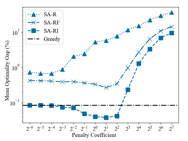
(b) $n=200$

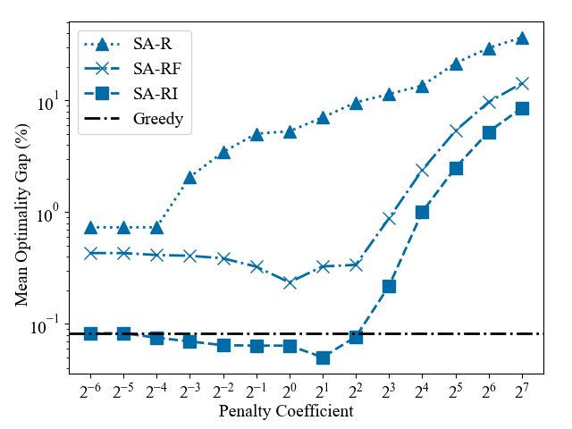
(c) $n=300$

Figure 5: Optimality gap for each problem size $n$ of QKP instances. Optimality gap for SA is plotted only for $\lambda$ producing feasible solutions on all instances. SA-RF denotes SA-R followed by fill-up operation, which produces locally optimal solutions. Fill-up operation improves solutions of SA-R particularly around $\lambda=2$, which is optimal penalty coefficient for SA-RI.

Appendix A Proof

We provide a proof of Proposition 1.

Proposition 2.

For a QKP instance defined as Eq. (II-B), an optimum is attained by a solution $x\in\{0,1\}^{n}$ satisfying $C-\max_{i}w_{i}<\sum_{i=1}^{n}w_{i}x_{i}\leq C$.

Proof.

Assume an optimal solution $x\in\{0,1\}^{n}$ satisfies $\sum_{i=1}^{n}w_{i}x_{i}\leq C-\max_{i}w_{i}$. We take another solution $\tilde{x}\in\{0,1\}^{n}$ obtained by changing the value of $x_{j}$ to $1$ for arbitrarily chosen $j$ such that $x_{j}=0$. Note that such $j$ exists since we assume $C<\sum_{i}w_{i}$. Note also that $\tilde{x}$ is a feasible solution since $\sum_{i=1}^{n}w_{i}\tilde{x}_{i}=\sum_{i=1}^{n}w_{i}x_{i}+w_{j}\leq C-\max_{i}w_{i}+w_{j}\leq C$. Let $\phi(x)$ denote the objective value for $x$. Since profits $p_{ij},p_{i}$ are non-negative, we have $\phi(x)\leq\phi(\tilde{x})$. Since $x$ is optimal, we get $\phi(x)=\phi(\tilde{x})$ and thus $\tilde{x}$ is also optimal. We replace $x$ with $\tilde{x}$ and repeat the same procedure, then we obtain an optimal solution satisfying $C-\max_{i}w_{i}<\sum_{i=1}^{n}w_{i}x_{i}\leq C$.

∎

Appendix B Full Results of Experiments

B-A Results on Simulated Annealing

Full results of the simulation experiments on medium-sized instances conducted in Section IV are shown in Table XI. In addition to the best objective value over 10 solutions obtained, we show a success rate, that is, the rate of the number of times to hit the optimum out of 10 executions, and the mean objective value. $\lambda$ denotes the optimal penalty coefficient for each method based on a lexicographic order for tuples of the best objective value, success rate, and mean objective value (e.g., if two values of $\lambda$ have the same best objective, then their success rates are compared). If multiple values of $\lambda$ obtain the same values for all metrics, then a smaller one is reported. ‘FS’ stands for the rate of feasible solutions over 10 outputs of SA. ‘Mean’ and ‘Best’ denote the mean and best objective values over 10 solutions for the optimal $\lambda$, respectively. ‘Gap’ is the optimality gap computed by the best objective value and known optimal value. ‘SR’ stands for a success rate. SR takes positive values only when Gap attains zero. Note that for instances that can be optimally solved by the greedy method, the optimal $\lambda$ for SA-RI takes the minimal value $2^{-6}$ among those tested. This is because an output of SA-RI under $\lambda\to 0$ coincides with that of the greedy algorithm as explained in Section III.

The results for SA-RF (SA-R followed by the fill-up operation) mentioned in Section IV for each $n$ is shown in Fig. 3. We see that for every case, the difference between SA-R and SA-RF is large around $\lambda=2$, which shows that SA could not obtain locally optimal solutions. We also conducted additional experiments with the end temperature of SA lowered to 0.01, and got almost the same results. This indicates that the inability to get locally optimal solutions cannot be easily resolved by tuning annealing schedules.

The full results of the performance comparison of SA-RI over various encoding methods conducted in Section IV-C are shown in Table XII. Beyond the similarity of averaged performance in the main text, we also see instance-wise similarity: if an instance cannot be optimally solved by some encoding method, there tends to be another encoding that cannot reach optimality on that instance. We also observe that the hybrid encoding has a relatively large optimality gap on instance 100_25_3, and so do the unary and offset encodings on instance 100_100_7. This is because the optima on these instances are small compared to other instances. Such a large optimality gap on one instance has a large effect on the mean values in Table VI. Due to this instability of the optimality gap as a performance metric, it might be hard to conclude the best encoding method for the proposed method.

We explain some details on the estimation of the optimal penalty coefficient $\lambda_{\text{SA-RI}}$ conducted in Section IV-D. We excluded instances that can be optimally solved by the greedy method, since the optimal values of $\lambda_{\text{SA-RI}}$ on those instances are trivially $0$ and so considered as the outlier value for the analysis. We used LinearRegression module in the scikit-learn library of version 1.2.2 for the regression.

To get insight into the behavior of the optimal penalty coefficient $\lambda$ for SA-RI, we plot the optimality gap for each instance on all $\lambda$ as a heat map in Fig. 6. Here we slightly modify the performance metric as

$$\text{Aggregated \ Optimality \ Gap}=$$

$$\frac{S_{\mathrm{best}}-S+(1-\mathrm{Success\ Rate})}{S_{\mathrm{best}}}\times 100\ (\%),$$

where $S$ is the best objective value obtained by SA-RI, Success Rate is the rate of hitting the optimum ($\leq 1$), and $S_{\rm best}$ is the known optimum. The aggregated optimality gap takes zero if and only if all solutions obtained are optimal. Note also that $\lambda$ minimizing the aggregated optimality gap corresponds (if it is unique) to $\lambda$ shown in Table XI since $S$ is an integer and Success Rate is less than 1 unless $S=S_{\rm best}$. In Fig. 6, good penalty coefficients correspond to an area of dark colors. We observe that the tested range of $\lambda$ is sufficiently wide to cover good penalty coefficients for each instance. We see a trend that the area slightly moves to the right as $d$ gets large, which agrees with the analysis result in Section IV-D.

TABLE XI: Full Results of Simulated Annealing.

Instance		Greedy			SA							SA-R						SA-I						SA-RI
$n$_$d$_id	Optimal	Score	Gap		$\lambda$	FS	Mean	Best	Gap	SR		$\lambda$	Mean	Best	Gap	SR		$\lambda$	Mean	Best	Gap	SR		$\lambda$	Mean	Best	Gap	SR
100_25_1	18558	18511	0.253		$2^{2}$	0.5	17063.40	17456	5.938	0.0		$2^{-1}$	18250.90	18514	0.237	0.0		$2^{2}$	18137.40	18325	1.256	0.0		$2^{-3}$	18558.00	18558	0.000	1.0
100_25_2	56525	56525	0.000		$2^{0}$	1.0	41780.10	48803	13.661	0.0		$2^{-6}$	55578.00	55578	1.675	0.0		$2^{-1}$	56491.10	56525	0.000	0.7		$2^{-6}$	56525.00	56525	0.000	1.0
100_25_3	3752	3702	1.333		$2^{3}$	0.4	3263.00	3646	2.825	0.0		$2^{3}$	3072.10	3646	2.825	0.0		$2^{3}$	3667.50	3752	0.000	0.1		$2^{3}$	3635.40	3752	0.000	0.1
100_25_4	50382	50382	0.000		$2^{-1}$	0.7	39337.29	44631	11.415	0.0		$2^{-6}$	50382.00	50382	0.000	1.0		$2^{-1}$	50356.14	50382	0.000	0.2		$2^{-6}$	50382.00	50382	0.000	1.0
100_25_5	61494	61494	0.000		$2^{-3}$	1.0	50121.40	53275	13.366	0.0		$2^{-6}$	60983.00	60983	0.831	0.0		$2^{-2}$	61465.50	61494	0.000	0.9		$2^{-6}$	61494.00	61494	0.000	1.0
100_25_6	36360	36189	0.470		$2^{2}$	0.7	32881.29	34982	3.790	0.0		$2^{-1}$	36131.50	36360	0.000	0.1		$2^{2}$	35939.43	36198	0.446	0.0		$2^{0}$	36206.90	36360	0.000	0.1
100_25_7	14657	14553	0.710		$2^{2}$	0.3	14082.00	14217	3.002	0.0		$2^{0}$	14312.40	14555	0.696	0.0		$2^{2}$	14338.00	14456	1.371	0.0		$2^{-3}$	14657.00	14657	0.000	1.0
100_25_8	20452	20307	0.709		$2^{2}$	0.3	18370.67	19544	4.440	0.0		$2^{0}$	19914.40	20106	1.692	0.0		$2^{2}$	20066.67	20337	0.562	0.0		$2^{1}$	20243.30	20355	0.474	0.0
100_25_9	35438	35365	0.206		$2^{1}$	0.6	30686.83	32783	7.492	0.0		$2^{-2}$	34871.70	35438	0.000	0.2		$2^{1}$	35311.83	35357	0.229	0.0		$2^{-2}$	35382.50	35438	0.000	0.4
100_25_10	24930	24926	0.016		$2^{1}$	0.3	24656.33	24784	0.586	0.0		$2^{-1}$	24763.00	24926	0.016	0.0		$2^{1}$	24854.00	24926	0.016	0.0		$2^{-1}$	24901.10	24930	0.000	0.1
100_50_1	83742	83712	0.036		$2^{2}$	0.7	68493.57	81874	2.231	0.0		$2^{0}$	76492.50	83168	0.685	0.0		$2^{2}$	83555.43	83742	0.000	0.4		$2^{2}$	83611.40	83742	0.000	0.7
100_50_2	104856	104770	0.082		$2^{0}$	0.8	83383.25	92819	11.480	0.0		$2^{-1}$	102182.20	104766	0.086	0.0		$2^{3}$	104567.60	104856	0.000	0.2		$2^{3}$	104567.60	104856	0.000	0.2
100_50_3	34006	33902	0.306		$2^{3}$	0.1	31130.00	31130	8.457	0.0		$2^{1}$	33462.00	33775	0.679	0.0		$2^{3}$	32738.00	32738	3.729	0.0		$2^{1}$	33936.20	34006	0.000	0.4
100_50_4	105996	105996	0.000		$2^{0}$	0.9	82037.33	94211	11.118	0.0		$2^{-6}$	105876.00	105876	0.113	0.0		$2^{1}$	105966.30	105996	0.000	0.8		$2^{-6}$	105996.00	105996	0.000	1.0
100_50_5	56464	56464	0.000		$2^{2}$	0.1	56227.00	56227	0.420	0.0		$2^{1}$	55846.90	56388	0.135	0.0		$2^{2}$	56398.00	56398	0.117	0.0		$2^{-6}$	56464.00	56464	0.000	1.0
100_50_6	16083	16083	0.000		$2^{3}$	0.1	15091.00	15091	6.168	0.0		$2^{-6}$	16080.00	16080	0.019	0.0		$2^{3}$	16083.00	16083	0.000	0.1		$2^{-6}$	16083.00	16083	0.000	1.0
100_50_7	52819	52784	0.066		$2^{3}$	0.3	44920.33	47827	9.451	0.0		$2^{-6}$	52646.00	52646	0.328	0.0		$2^{3}$	49795.67	50240	4.883	0.0		$2^{1}$	52687.30	52819	0.000	0.3
100_50_8	54246	54030	0.398		$2^{2}$	0.1	52562.00	52562	3.104	0.0		$2^{0}$	53946.30	54176	0.129	0.0		$2^{2}$	53408.00	53408	1.545	0.0		$2^{0}$	54166.00	54246	0.000	0.3
100_50_9	68974	68974	0.000		$2^{1}$	0.2	62401.00	68974	0.000	0.1		$2^{-6}$	68974.00	68974	0.000	1.0		$2^{1}$	68974.00	68974	0.000	0.2		$2^{-6}$	68974.00	68974	0.000	1.0
100_50_10	88634	88527	0.121		$2^{3}$	1.0	63369.90	78751	11.150	0.0		$2^{0}$	68151.10	88146	0.551	0.0		$2^{3}$	88505.20	88634	0.000	0.1		$2^{3}$	88505.20	88634	0.000	0.1
100_75_1	189137	189137	0.000		$2^{-1}$	1.0	141711.30	163058	13.788	0.0		$2^{-6}$	189137.00	189137	0.000	1.0		$2^{-1}$	189137.00	189137	0.000	1.0		$2^{-6}$	189137.00	189137	0.000	1.0
100_75_2	95074	94980	0.099		$2^{3}$	0.6	77125.33	90450	4.864	0.0		$2^{0}$	94276.70	94822	0.265	0.0		$2^{2}$	94980.00	94980	0.099	0.0		$2^{2}$	94956.70	95074	0.000	0.1
100_75_3	62098	62098	0.000		$2^{4}$	0.3	52999.67	53802	13.360	0.0		$2^{1}$	62061.60	62098	0.000	0.3		$2^{4}$	55379.33	56115	9.635	0.0		$2^{-6}$	62098.00	62098	0.000	1.0
100_75_4	72245	72167	0.108		$2^{3}$	0.3	68158.00	69522	3.769	0.0		$2^{0}$	71302.90	71995	0.346	0.0		$2^{3}$	70151.33	70843	1.941	0.0		$2^{2}$	72029.40	72245	0.000	0.3
100_75_5	27616	27616	0.000		$2^{3}$	0.1	27543.00	27543	0.264	0.0		$2^{1}$	27354.40	27557	0.214	0.0		$2^{3}$	27616.00	27616	0.000	0.1		$2^{-6}$	27616.00	27616	0.000	1.0
100_75_6	145273	145224	0.034		$2^{2}$	0.9	116283.78	144022	0.861	0.0		$2^{0}$	131337.00	144746	0.363	0.0		$2^{3}$	143779.20	145273	0.000	0.1		$2^{3}$	143779.20	145273	0.000	0.1
100_75_7	110979	110451	0.476		$2^{3}$	0.8	88068.50	106227	4.282	0.0		$2^{0}$	110477.10	110718	0.235	0.0		$2^{3}$	110283.62	110937	0.038	0.0		$2^{1}$	110910.70	110979	0.000	0.5
100_75_8	19570	19570	0.000		$2^{2}$	0.2	19547.50	19570	0.000	0.1		$2^{2}$	18693.60	19570	0.000	0.1		$2^{2}$	19570.00	19570	0.000	0.2		$2^{-6}$	19570.00	19570	0.000	1.0
100_75_9	104341	103916	0.407		$2^{3}$	0.8	85243.88	100546	3.637	0.0		$2^{0}$	103036.60	103655	0.657	0.0		$2^{3}$	102979.00	104148	0.185	0.0		$2^{2}$	103934.40	104253	0.084	0.0
100_75_10	143740	143695	0.031		$2^{1}$	0.9	108421.11	124507	13.380	0.0		$2^{0}$	119219.30	143740	0.000	0.1		$2^{1}$	143721.56	143740	0.000	0.7		$2^{1}$	143600.40	143740	0.000	0.7
100_100_1	81978	81961	0.021		$2^{4}$	0.1	75824.00	75824	7.507	0.0		$2^{2}$	81867.40	81961	0.021	0.0		$2^{5}$	75186.80	80348	1.988	0.0		$2^{3}$	81803.60	81978	0.000	0.1
100_100_2	190424	189998	0.224		$2^{1}$	0.7	148425.86	167736	11.914	0.0		$2^{0}$	167000.80	190338	0.045	0.0		$2^{0}$	190170.40	190424	0.000	0.1		$2^{0}$	190230.50	190424	0.000	0.1
100_100_3	225434	225434	0.000		$2^{1}$	1.0	167360.40	201873	10.451	0.0		$2^{-1}$	211582.00	225434	0.000	0.4		$2^{1}$	225434.00	225434	0.000	1.0		$2^{-6}$	225434.00	225434	0.000	1.0
100_100_4	63028	63028	0.000		$2^{4}$	0.1	54077.00	54077	14.202	0.0		$2^{-6}$	63028.00	63028	0.000	1.0		$2^{5}$	53484.75	58212	7.641	0.0		$2^{-6}$	63028.00	63028	0.000	1.0
100_100_5	230076	230076	0.000		$2^{0}$	0.6	166587.67	184411	19.848	0.0		$2^{-6}$	229660.00	229660	0.181	0.0		$2^{2}$	230070.20	230076	0.000	0.9		$2^{-6}$	230076.00	230076	0.000	1.0
100_100_6	74358	74358	0.000		$2^{4}$	0.1	68717.00	68717	7.586	0.0		$2^{1}$	74035.30	74103	0.343	0.0		$2^{3}$	74358.00	74358	0.000	0.1		$2^{-6}$	74358.00	74358	0.000	1.0
100_100_7	10330	10184	1.413		$2^{5}$	0.2	8249.50	9664	6.447	0.0		$2^{-6}$	10108.00	10108	2.149	0.0		$2^{6}$	8256.86	9731	5.799	0.0		$2^{5}$	9717.40	10330	0.000	0.1
100_100_8	62582	62422	0.256		$2^{3}$	0.2	62427.00	62457	0.200	0.0		$2^{1}$	62274.30	62484	0.157	0.0		$2^{3}$	62582.00	62582	0.000	0.2		$2^{3}$	62509.90	62582	0.000	0.6
100_100_9	232754	232693	0.026		$2^{1}$	1.0	164711.60	208886	10.255	0.0		$2^{-6}$	231402.00	231402	0.581	0.0		$2^{6}$	232741.80	232754	0.000	0.8		$2^{6}$	232741.80	232754	0.000	0.8
100_100_10	193262	193218	0.023		$2^{2}$	0.8	138825.50	166966	13.606	0.0		$2^{1}$	142628.90	192352	0.471	0.0		$2^{4}$	193174.10	193262	0.000	0.5		$2^{4}$	193174.10	193262	0.000	0.5
200_25_1	204441	204399	0.021		$2^{-1}$	1.0	156096.80	180652	11.636	0.0		$2^{-6}$	203061.00	203061	0.675	0.0		$2^{-1}$	204397.00	204441	0.000	0.2		$2^{-1}$	204402.20	204441	0.000	0.2
200_25_2	239573	239573	0.000		$2^{-3}$	0.7	184058.14	199793	16.605	0.0		$2^{-6}$	238734.00	238734	0.350	0.0		$2^{-2}$	239564.00	239573	0.000	0.4		$2^{-6}$	239573.00	239573	0.000	1.0
200_25_3	245463	244446	0.414		$2^{-3}$	1.0	192841.00	223037	9.136	0.0		$2^{-6}$	243967.00	243967	0.609	0.0		$2^{4}$	244828.60	245463	0.000	0.2		$2^{4}$	244828.60	245463	0.000	0.2
200_25_4	222361	221591	0.346		$2^{-1}$	1.0	160720.70	198848	10.574	0.0		$2^{-6}$	221054.00	221054	0.588	0.0		$2^{-2}$	222314.20	222361	0.000	0.8		$2^{-2}$	222314.20	222361	0.000	0.8
200_25_5	187324	187315	4.8E-3		$2^{1}$	1.0	145902.90	173607	7.323	0.0		$2^{-2}$	168024.20	186861	0.247	0.0		$2^{0}$	187256.80	187324	0.000	0.4		$2^{0}$	187256.80	187324	0.000	0.4
200_25_6	80351	80276	0.093		$2^{2}$	0.1	75841.00	75841	5.613	0.0		$2^{-5}$	80229.00	80229	0.152	0.0		$2^{2}$	78282.00	78282	2.575	0.0		$2^{-2}$	80279.40	80310	0.051	0.0
200_25_7	59036	58858	0.302		$2^{3}$	0.2	52897.50	53754	8.947	0.0		$2^{0}$	58597.30	59002	0.058	0.0		$2^{3}$	55971.00	56795	3.796	0.0		$2^{1}$	58938.20	59036	0.000	0.5
200_25_8	149433	149125	0.206		$2^{3}$	1.0	128227.00	141491	5.315	0.0		$2^{0}$	143627.50	148952	0.322	0.0		$2^{1}$	149319.50	149384	0.033	0.0		$2^{-1}$	149208.20	149433	0.000	0.2
200_25_9	49366	49366	0.000		$2^{3}$	0.3	44759.33	45303	8.230	0.0		$2^{-6}$	49293.00	49293	0.148	0.0		$2^{3}$	47749.00	47984	2.799	0.0		$2^{-6}$	49366.00	49366	0.000	1.0
200_25_10	48459	48291	0.347		$2^{3}$	0.3	41439.67	43291	10.665	0.0		$2^{0}$	48267.20	48412	0.097	0.0		$2^{3}$	45235.00	45870	5.343	0.0		$2^{0}$	48358.20	48459	0.000	0.4

TABLE XI: Full Results of Simulated Annealing (Continued).

Instance		Greedy			SA							SA-R						SA-I						SA-RI
$n$_$d$_id	Optimal	Score	Gap		$\lambda$	FS	Mean	Best	Gap	SR		$\lambda$	Mean	Best	Gap	SR		$\lambda$	Mean	Best	Gap	SR		$\lambda$	Mean	Best	Gap	SR
200_50_1	372097	372097	0.000		$2^{0}$	0.9	294501.33	326397	12.282	0.0		$2^{-6}$	372097.00	372097	0.000	1.0		$2^{1}$	372097.00	372097	0.000	0.9		$2^{-6}$	372097.00	372097	0.000	1.0
200_50_2	211130	210485	0.305		$2^{4}$	0.3	176418.67	193428	8.384	0.0		$2^{1}$	209220.60	210624	0.240	0.0		$2^{4}$	202804.00	205228	2.795	0.0		$2^{1}$	210838.30	211090	0.019	0.0
200_50_3	227185	227185	0.000		$2^{4}$	0.3	205635.67	214039	5.786	0.0		$2^{1}$	226135.00	226428	0.333	0.0		$2^{3}$	225172.00	225172	0.886	0.0		$2^{-6}$	227185.00	227185	0.000	1.0
200_50_4	228572	228572	0.000		$2^{3}$	0.1	219575.00	219575	3.936	0.0		$2^{-6}$	228572.00	228572	0.000	1.0		$2^{3}$	223641.00	223641	2.157	0.0		$2^{-6}$	228572.00	228572	0.000	1.0
200_50_5	479651	479451	0.042		$2^{-2}$	0.9	370026.67	426263	11.131	0.0		$2^{-6}$	479004.00	479004	0.135	0.0		$2^{7}$	479436.40	479451	0.042	0.0		$2^{-6}$	479451.00	479451	0.042	0.0
200_50_6	426777	426436	0.080		$2^{-2}$	0.5	347722.20	348287	18.391	0.0		$2^{-6}$	425835.00	425835	0.221	0.0		$2^{-2}$	426657.00	426657	0.028	0.0		$2^{-1}$	426601.20	426657	0.028	0.0
200_50_7	220890	220806	0.038		$2^{3}$	0.1	201893.00	201893	8.600	0.0		$2^{-1}$	218989.00	220456	0.196	0.0		$2^{2}$	220842.00	220842	0.022	0.0		$2^{0}$	220683.20	220842	0.022	0.0
200_50_8	317952	317880	0.023		$2^{3}$	1.0	256469.50	288786	9.173	0.0		$2^{-1}$	317150.10	317742	0.066	0.0		$2^{0}$	317952.00	317952	0.000	0.1		$2^{-3}$	317952.00	317952	0.000	1.0
200_50_9	104936	104936	0.000		$2^{4}$	0.3	95284.33	98644	5.996	0.0		$2^{1}$	103506.60	104913	0.022	0.0		$2^{4}$	99015.33	101660	3.122	0.0		$2^{-6}$	104936.00	104936	0.000	1.0
200_50_10	284751	284741	3.5E-3		$2^{3}$	0.7	259466.86	277449	2.564	0.0		$2^{0}$	281643.60	284741	3.5E-3	0.0		$2^{2}$	283984.00	283984	0.269	0.0		$2^{2}$	284054.30	284751	0.000	0.1
200_75_1	442894	442423	0.106		$2^{4}$	0.7	383841.14	426329	3.740	0.0		$2^{0}$	439884.10	441263	0.368	0.0		$2^{4}$	437349.86	442602	0.066	0.0		$2^{2}$	441433.60	442862	7.2E-3	0.0
200_75_2	286643	286632	3.8E-3		$2^{4}$	0.2	268944.00	274508	4.233	0.0		$2^{1}$	284667.30	286615	9.8E-3	0.0		$2^{4}$	279890.50	281342	1.849	0.0		$2^{2}$	286183.10	286643	0.000	0.2
200_75_3	61924	61924	0.000		$2^{5}$	0.1	59806.00	59806	3.420	0.0		$2^{3}$	61171.00	61475	0.725	0.0		$2^{5}$	60365.00	60365	2.518	0.0		$2^{-6}$	61924.00	61924	0.000	1.0
200_75_4	128351	128351	0.000		$2^{5}$	0.3	94229.67	96894	24.509	0.0		$2^{1}$	128196.50	128351	0.000	0.6		$2^{5}$	102443.67	104265	18.766	0.0		$2^{-6}$	128351.00	128351	0.000	1.0
200_75_5	137885	137764	0.088		$2^{5}$	0.3	120425.00	123930	10.121	0.0		$2^{2}$	137000.80	137690	0.141	0.0		$2^{5}$	125643.00	127511	7.524	0.0		$2^{3}$	137751.30	137885	0.000	0.2
200_75_6	229631	229250	0.166		$2^{5}$	0.1	204220.00	204220	11.066	0.0		$2^{2}$	227701.70	229186	0.194	0.0		$2^{5}$	215268.00	215268	6.255	0.0		$2^{2}$	229316.40	229631	0.000	0.4
200_75_7	269887	269887	0.000		$2^{4}$	0.1	255693.00	255693	5.259	0.0		$2^{1}$	267588.90	269558	0.122	0.0		$2^{4}$	261943.00	261943	2.943	0.0		$2^{-6}$	269887.00	269887	0.000	1.0
200_75_8	600858	600806	8.7E-3		$2^{0}$	1.0	451760.70	530210	11.758	0.0		$2^{-6}$	600659.00	600659	0.033	0.0		$2^{0}$	599597.40	600858	0.000	0.2		$2^{0}$	599597.40	600858	0.000	0.2
200_75_9	516771	516151	0.120		$2^{2}$	0.9	420729.67	482853	6.563	0.0		$2^{0}$	494623.20	515058	0.331	0.0		$2^{-1}$	516494.00	516494	0.054	0.0		$2^{1}$	516395.70	516661	0.021	0.0
200_75_10	142694	142694	0.000		$2^{4}$	0.1	134749.00	134749	5.568	0.0		$2^{2}$	141502.70	142585	0.076	0.0		$2^{4}$	138983.00	138983	2.601	0.0		$2^{-6}$	142694.00	142694	0.000	1.0
200_100_1	937149	937123	2.8E-3		$2^{-1}$	0.7	717350.86	778851	16.891	0.0		$2^{-6}$	935700.00	935700	0.155	0.0		$2^{4}$	937093.10	937149	0.000	0.3		$2^{4}$	937093.10	937149	0.000	0.3
200_100_2	303058	302690	0.121		$2^{6}$	0.5	237593.60	250511	17.339	0.0		$2^{2}$	301369.40	302035	0.338	0.0		$2^{6}$	246849.60	257617	14.994	0.0		$2^{4}$	301856.00	303050	2.6E-3	0.0
200_100_3	29367	29296	0.242		$2^{6}$	0.2	27624.00	27834	5.220	0.0		$2^{4}$	28956.90	29176	0.650	0.0		$2^{6}$	28285.00	28285	3.684	0.0		$2^{-6}$	29296.00	29296	0.242	0.0
200_100_4	100838	100838	0.000		$2^{5}$	0.1	93818.00	93818	6.962	0.0		$2^{3}$	100508.50	100837	9.9E-4	0.0		$2^{5}$	95446.00	95446	5.347	0.0		$2^{-6}$	100838.00	100838	0.000	1.0
200_100_5	786635	786482	0.019		$2^{1}$	0.9	586694.89	689990	12.286	0.0		$2^{1}$	606642.30	786169	0.059	0.0		$2^{4}$	786458.40	786490	0.018	0.0		$2^{4}$	786458.40	786490	0.018	0.0
200_100_6	41171	41171	0.000		$2^{6}$	0.1	39199.00	39199	4.790	0.0		$2^{4}$	39688.60	41171	0.000	0.2		$2^{6}$	39980.00	39980	2.893	0.0		$2^{-6}$	41171.00	41171	0.000	1.0
200_100_7	701094	700965	0.018		$2^{1}$	0.6	540193.33	609513	13.063	0.0		$2^{1}$	604114.80	700570	0.075	0.0		$2^{1}$	700970.50	700998	0.014	0.0		$2^{1}$	700993.00	701094	0.000	0.2
200_100_8	782443	781455	0.126		$2^{1}$	1.0	597174.90	693221	11.403	0.0		$2^{-6}$	779797.00	779797	0.338	0.0		$2^{3}$	781926.60	782408	4.5E-3	0.0		$2^{3}$	781926.60	782408	4.5E-3	0.0
200_100_9	628992	628893	0.016		$2^{3}$	0.8	546637.50	582449	7.400	0.0		$2^{0}$	626696.10	627799	0.190	0.0		$2^{3}$	627774.00	628992	0.000	0.1		$2^{2}$	627240.90	628992	0.000	0.1
200_100_10	378442	378169	0.072		$2^{5}$	0.4	340558.25	347358	8.214	0.0		$2^{2}$	376514.00	377460	0.259	0.0		$2^{5}$	355961.50	363794	3.871	0.0		$2^{-6}$	378169.00	378169	0.072	0.0
300_25_1	29140	29140	0.000		$2^{5}$	0.4	24376.50	25337	13.051	0.0		$2^{2}$	28985.20	29104	0.124	0.0		$2^{5}$	26907.75	27951	4.080	0.0		$2^{-6}$	29140.00	29140	0.000	1.0
300_25_2	281990	281268	0.256		$2^{2}$	0.3	265680.00	279136	1.012	0.0		$2^{-1}$	280505.20	281931	0.021	0.0		$2^{2}$	280874.33	281077	0.324	0.0		$2^{0}$	281882.10	281973	6.0E-3	0.0
300_25_3	231075	231075	0.000		$2^{3}$	0.1	205225.00	205225	11.187	0.0		$2^{-1}$	230662.90	231075	0.000	0.3		$2^{3}$	226661.00	226661	1.910	0.0		$2^{-6}$	231075.00	231075	0.000	1.0
300_25_4	444759	444712	0.011		$2^{-2}$	1.0	333689.10	377515	15.119	0.0		$2^{-6}$	443909.00	443909	0.191	0.0		$2^{-2}$	444559.20	444725	7.6E-3	0.0		$2^{-2}$	444559.20	444725	7.6E-3	0.0
300_25_5	14988	14879	0.727		$2^{5}$	0.2	12814.50	13524	9.768	0.0		$2^{3}$	14729.90	14958	0.200	0.0		$2^{5}$	13494.00	14245	4.957	0.0		$2^{3}$	14894.40	14988	0.000	0.1
300_25_6	269782	269671	0.041		$2^{3}$	0.3	256370.00	257802	4.441	0.0		$2^{-1}$	267575.50	269671	0.041	0.0		$2^{3}$	263143.00	263753	2.235	0.0		$2^{1}$	269338.00	269782	0.000	0.3
300_25_7	485263	484539	0.149		$2^{-4}$	0.6	373124.17	378224	22.058	0.0		$2^{-6}$	483078.00	483078	0.450	0.0		$2^{1}$	484619.00	485263	0.000	0.1		$2^{1}$	484619.00	485263	0.000	0.1
300_25_8	9343	9343	0.000		$2^{6}$	0.6	7148.50	8223	11.988	0.0		$2^{-6}$	9224.00	9224	1.274	0.0		$2^{6}$	8061.83	8863	5.138	0.0		$2^{-6}$	9343.00	9343	0.000	1.0
300_25_9	250761	250551	0.084		$2^{3}$	0.3	238705.67	243136	3.041	0.0		$2^{-1}$	250406.50	250751	4.0E-3	0.0		$2^{3}$	248275.33	248900	0.742	0.0		$2^{1}$	250398.50	250761	0.000	0.1
300_25_10	383377	383377	0.000		$2^{0}$	0.9	309068.11	347659	9.317	0.0		$2^{-1}$	331814.50	383377	0.000	0.1		$2^{0}$	382790.67	383377	0.000	0.2		$2^{-6}$	383377.00	383377	0.000	1.0
300_50_1	513379	513361	3.5E-3		$2^{4}$	0.4	470796.75	483335	5.852	0.0		$2^{1}$	511127.00	512984	0.077	0.0		$2^{2}$	513084.00	513084	0.057	0.0		$2^{1}$	513057.50	513379	0.000	0.1
300_50_2	105543	105543	0.000		$2^{5}$	0.2	90216.00	95103	9.892	0.0		$2^{2}$	103926.40	105543	0.000	0.3		$2^{5}$	95996.50	99371	5.848	0.0		$2^{-6}$	105543.00	105543	0.000	1.0
300_50_3	875788	874561	0.140		$2^{-1}$	1.0	665029.60	745587	14.867	0.0		$2^{-6}$	871417.00	871417	0.499	0.0		$2^{0}$	875387.40	875769	2.2E-3	0.0		$2^{0}$	875387.40	875769	2.2E-3	0.0
300_50_4	307124	307124	0.000		$2^{5}$	0.3	265725.00	270113	12.051	0.0		$2^{-6}$	306937.00	306937	0.061	0.0		$2^{5}$	281834.00	285461	7.054	0.0		$2^{-6}$	307124.00	307124	0.000	1.0
300_50_5	727820	727486	0.046		$2^{1}$	0.9	616767.22	655825	9.892	0.0		$2^{-1}$	726349.50	727463	0.049	0.0		$2^{0}$	727650.00	727684	0.019	0.0		$2^{1}$	727634.60	727820	0.000	0.1
300_50_6	734053	733855	0.027		$2^{1}$	0.9	619285.56	662004	9.815	0.0		$2^{0}$	662379.00	733923	0.018	0.0		$2^{2}$	733833.10	734053	0.000	0.1		$2^{0}$	733963.40	734053	0.000	0.1
300_50_7	43595	43524	0.163		$2^{6}$	0.3	31501.33	33915	22.204	0.0		$2^{3}$	42913.00	43203	0.899	0.0		$2^{6}$	35597.00	37920	13.018	0.0		$2^{4}$	43479.40	43595	0.000	0.2
300_50_8	767977	767959	2.3E-3		$2^{0}$	0.7	640103.00	703023	8.458	0.0		$2^{0}$	678100.80	767311	0.087	0.0		$2^{3}$	766792.70	767960	2.2E-3	0.0		$2^{3}$	766792.70	767960	2.2E-3	0.0
300_50_9	761351	761351	0.000		$2^{1}$	0.8	642154.75	689821	9.395	0.0		$2^{-6}$	760565.00	760565	0.103	0.0		$2^{0}$	761154.12	761351	0.000	0.2		$2^{-6}$	761351.00	761351	0.000	1.0
300_50_10	996070	996070	0.000		$2^{-2}$	1.0	710165.70	887845	10.865	0.0		$2^{-6}$	989559.00	989559	0.654	0.0		$2^{5}$	994305.30	996070	0.000	0.1		$2^{-6}$	996070.00	996070	0.000	1.0

TABLE XII: Full Results of SA-RI with Various Encoding Methods.

Instance			Binary						Hybrid						Unary						One-hot						Offset
$n$_$d$_id	Optimal		$\lambda$	Mean	Best	Gap	SR		$\lambda$	Mean	Best	Gap	SR		$\lambda$	Mean	Best	Gap	SR		$\lambda$	Mean	Best	Gap	SR		$\lambda$	Mean	Best	Gap	SR
100_25_1	18558		$2^{-3}$	18558.0	18558	0.000	1.0		$2^{-3}$	18558.0	18558	0.000	1.0		$2^{-3}$	18558.0	18558	0.000	1.0		$2^{-4}$	18558.0	18558	0.000	1.0		$2^{-4}$	18558.0	18558	0.000	1.0
100_25_2	56525		$2^{-6}$	56525.0	56525	0.000	1.0		$2^{-6}$	56525.0	56525	0.000	1.0		$2^{-6}$	56525.0	56525	0.000	1.0		$2^{-6}$	56525.0	56525	0.000	1.0		$2^{-6}$	56525.0	56525	0.000	1.0
100_25_3	3752		$2^{3}$	3664.4	3752	0.000	0.2		$2^{1}$	3705.0	3717	0.933	0.0		$2^{3}$	3532.2	3752	0.000	0.1		$2^{3}$	3562.3	3752	0.000	0.1		$2^{3}$	3582.6	3752	0.000	0.1
100_25_4	50382		$2^{-6}$	50382.0	50382	0.000	1.0		$2^{-6}$	50382.0	50382	0.000	1.0		$2^{-6}$	50382.0	50382	0.000	1.0		$2^{-6}$	50382.0	50382	0.000	1.0		$2^{-6}$	50382.0	50382	0.000	1.0
100_25_5	61494		$2^{-6}$	61494.0	61494	0.000	1.0		$2^{-6}$	61494.0	61494	0.000	1.0		$2^{-6}$	61494.0	61494	0.000	1.0		$2^{-6}$	61494.0	61494	0.000	1.0		$2^{-6}$	61494.0	61494	0.000	1.0
100_25_6	36360		$2^{-1}$	36206.1	36360	0.000	0.1		$2^{-1}$	36223.2	36360	0.000	0.2		$2^{1}$	36169.3	36303	0.157	0.0		$2^{-1}$	36225.2	36360	0.000	0.2		$2^{0}$	36200.2	36360	0.000	0.1
100_25_7	14657		$2^{-3}$	14657.0	14657	0.000	1.0		$2^{-3}$	14657.0	14657	0.000	1.0		$2^{-3}$	14657.0	14657	0.000	1.0		$2^{-3}$	14657.0	14657	0.000	1.0		$2^{-3}$	14657.0	14657	0.000	1.0
100_25_8	20452		$2^{0}$	20290.9	20452	0.000	0.2		$2^{0}$	20286.2	20452	0.000	0.1		$2^{1}$	20319.4	20395	0.279	0.0		$2^{1}$	20330.2	20452	0.000	0.3		$2^{1}$	20304.9	20452	0.000	0.2
100_25_9	35438		$2^{-2}$	35401.6	35438	0.000	0.6		$2^{-2}$	35401.6	35438	0.000	0.6		$2^{-1}$	35370.3	35438	0.000	0.4		$2^{-3}$	35385.6	35438	0.000	0.5		$2^{-4}$	35438.0	35438	0.000	1.0
100_25_10	24930		$2^{-1}$	24909.8	24930	0.000	0.1		$2^{0}$	24904.7	24930	0.000	0.2		$2^{0}$	24901.4	24930	0.000	0.2		$2^{1}$	24864.0	24930	0.000	0.3		$2^{-2}$	24926.4	24930	0.000	0.1
100_50_1	83742		$2^{1}$	83695.7	83742	0.000	0.5		$2^{2}$	83361.3	83742	0.000	0.4		$2^{1}$	83711.9	83742	0.000	0.5		$2^{2}$	83190.4	83742	0.000	0.4		$2^{1}$	83736.0	83742	0.000	0.8
100_50_2	104856		$2^{1}$	104775.1	104856	0.000	0.1		$2^{1}$	104776.5	104792	0.061	0.0		$2^{1}$	104774.7	104792	0.061	0.0		$2^{1}$	104749.7	104856	0.000	0.1		$2^{-1}$	104751.2	104792	0.061	0.0
100_50_3	34006		$2^{1}$	33930.0	34006	0.000	0.5		$2^{0}$	33933.2	34006	0.000	0.3		$2^{0}$	33933.2	34006	0.000	0.3		$2^{2}$	33969.6	34006	0.000	0.5		$2^{2}$	33875.8	34006	0.000	0.3
100_50_4	105996		$2^{-6}$	105996.0	105996	0.000	1.0		$2^{-6}$	105996.0	105996	0.000	1.0		$2^{-6}$	105996.0	105996	0.000	1.0		$2^{-6}$	105996.0	105996	0.000	1.0		$2^{-6}$	105996.0	105996	0.000	1.0
100_50_5	56464		$2^{-6}$	56464.0	56464	0.000	1.0		$2^{-6}$	56464.0	56464	0.000	1.0		$2^{-6}$	56464.0	56464	0.000	1.0		$2^{-6}$	56464.0	56464	0.000	1.0		$2^{-6}$	56464.0	56464	0.000	1.0
100_50_6	16083		$2^{-6}$	16083.0	16083	0.000	1.0		$2^{-6}$	16083.0	16083	0.000	1.0		$2^{-6}$	16083.0	16083	0.000	1.0		$2^{-6}$	16083.0	16083	0.000	1.0		$2^{-6}$	16083.0	16083	0.000	1.0
100_50_7	52819		$2^{2}$	52347.7	52819	0.000	0.2		$2^{1}$	52735.7	52819	0.000	0.4		$2^{0}$	52787.5	52819	0.000	0.1		$2^{1}$	52760.1	52819	0.000	0.2		$2^{0}$	52697.5	52819	0.000	0.3
100_50_8	54246		$2^{0}$	54089.4	54246	0.000	0.2		$2^{2}$	53755.0	54246	0.000	0.1		$2^{2}$	53480.8	54246	0.000	0.1		$2^{2}$	53889.0	54246	0.000	0.3		$2^{1}$	54144.4	54246	0.000	0.2
100_50_9	68974		$2^{-6}$	68974.0	68974	0.000	1.0		$2^{-6}$	68974.0	68974	0.000	1.0		$2^{-6}$	68974.0	68974	0.000	1.0		$2^{-6}$	68974.0	68974	0.000	1.0		$2^{-6}$	68974.0	68974	0.000	1.0
100_50_10	88634		$2^{0}$	88470.4	88600	0.038	0.0		$2^{0}$	88507.4	88634	0.000	0.2		$2^{0}$	88528.5	88634	0.000	0.1		$2^{0}$	88492.2	88575	0.067	0.0		$2^{2}$	88346.8	88634	0.000	0.2
100_75_1	189137		$2^{-6}$	189137.0	189137	0.000	1.0		$2^{-6}$	189137.0	189137	0.000	1.0		$2^{-6}$	189137.0	189137	0.000	1.0		$2^{-6}$	189137.0	189137	0.000	1.0		$2^{-6}$	189137.0	189137	0.000	1.0
100_75_2	95074		$2^{2}$	94970.1	95074	0.000	0.1		$2^{0}$	94968.1	95003	0.075	0.0		$2^{-1}$	94978.9	95003	0.075	0.0		$2^{-1}$	94982.3	95003	0.075	0.0		$2^{-1}$	94988.6	95003	0.075	0.0
100_75_3	62098		$2^{-6}$	62098.0	62098	0.000	1.0		$2^{-6}$	62098.0	62098	0.000	1.0		$2^{-6}$	62098.0	62098	0.000	1.0		$2^{-6}$	62098.0	62098	0.000	1.0		$2^{-6}$	62098.0	62098	0.000	1.0
100_75_4	72245		$2^{1}$	72113.1	72245	0.000	0.2		$2^{2}$	72097.2	72245	0.000	0.1		$2^{2}$	72134.7	72245	0.000	0.4		$2^{1}$	72053.0	72245	0.000	0.2		$2^{0}$	72136.8	72245	0.000	0.3
100_75_5	27616		$2^{-6}$	27616.0	27616	0.000	1.0		$2^{-6}$	27616.0	27616	0.000	1.0		$2^{-6}$	27616.0	27616	0.000	1.0		$2^{-6}$	27616.0	27616	0.000	1.0		$2^{-6}$	27616.0	27616	0.000	1.0
100_75_6	145273		$2^{1}$	144452.1	145273	0.000	0.1		$2^{1}$	144995.9	145273	0.000	0.1		$2^{1}$	145049.0	145273	0.000	0.3		$2^{1}$	145104.7	145273	0.000	0.1		$2^{1}$	144143.2	145273	0.000	0.1
100_75_7	110979		$2^{1}$	110824.5	110979	0.000	0.3		$2^{2}$	110412.9	110979	0.000	0.2		$2^{1}$	110802.9	110979	0.000	0.2		$2^{1}$	110910.8	110979	0.000	0.5		$2^{1}$	110873.5	110979	0.000	0.4
100_75_8	19570		$2^{-6}$	19570.0	19570	0.000	1.0		$2^{-6}$	19570.0	19570	0.000	1.0		$2^{-6}$	19570.0	19570	0.000	1.0		$2^{-6}$	19570.0	19570	0.000	1.0		$2^{-6}$	19570.0	19570	0.000	1.0
100_75_9	104341		$2^{2}$	104028.4	104285	0.054	0.0		$2^{2}$	104078.8	104253	0.084	0.0		$2^{2}$	103668.9	104253	0.084	0.0		$2^{2}$	104138.8	104300	0.039	0.0		$2^{2}$	103659.2	104300	0.039	0.0
100_75_10	143740		$2^{2}$	143457.8	143740	0.000	0.6		$2^{2}$	143318.1	143740	0.000	0.6		$2^{2}$	143575.6	143740	0.000	0.7		$2^{2}$	143472.4	143740	0.000	0.7		$2^{2}$	143149.9	143740	0.000	0.4
100_100_1	81978		$2^{-6}$	81961.0	81961	0.021	0.0		$2^{-6}$	81961.0	81961	0.021	0.0		$2^{3}$	81962.7	81978	0.000	0.1		$2^{3}$	81801.4	81978	0.000	0.1		$2^{-6}$	81961.0	81961	0.021	0.0
100_100_2	190424		$2^{0}$	190301.4	190385	0.020	0.0		$2^{2}$	190221.7	190385	0.020	0.0		$2^{0}$	190262.7	190385	0.020	0.0		$2^{2}$	189529.8	190385	0.020	0.0		$2^{0}$	190241.0	190385	0.020	0.0
100_100_3	225434		$2^{-6}$	225434.0	225434	0.000	1.0		$2^{-6}$	225434.0	225434	0.000	1.0		$2^{-6}$	225434.0	225434	0.000	1.0		$2^{-6}$	225434.0	225434	0.000	1.0		$2^{-6}$	225434.0	225434	0.000	1.0
100_100_4	63028		$2^{-6}$	63028.0	63028	0.000	1.0		$2^{-6}$	63028.0	63028	0.000	1.0		$2^{-6}$	63028.0	63028	0.000	1.0		$2^{-6}$	63028.0	63028	0.000	1.0		$2^{-6}$	63028.0	63028	0.000	1.0
100_100_5	230076		$2^{-6}$	230076.0	230076	0.000	1.0		$2^{-6}$	230076.0	230076	0.000	1.0		$2^{-6}$	230076.0	230076	0.000	1.0		$2^{-6}$	230076.0	230076	0.000	1.0		$2^{-6}$	230076.0	230076	0.000	1.0
100_100_6	74358		$2^{-6}$	74358.0	74358	0.000	1.0		$2^{-6}$	74358.0	74358	0.000	1.0		$2^{-6}$	74358.0	74358	0.000	1.0		$2^{-6}$	74358.0	74358	0.000	1.0		$2^{-6}$	74358.0	74358	0.000	1.0
100_100_7	10330		$2^{5}$	10037.3	10330	0.000	0.2		$2^{5}$	9658.8	10330	0.000	0.2		$2^{-6}$	10184.0	10184	1.413	0.0		$2^{5}$	10083.3	10330	0.000	0.3		$2^{-6}$	10184.0	10184	1.413	0.0
100_100_8	62582		$2^{3}$	62481.0	62582	0.000	0.4		$2^{3}$	62499.5	62582	0.000	0.5		$2^{3}$	62084.8	62582	0.000	0.4		$2^{3}$	62131.2	62582	0.000	0.3		$2^{3}$	61924.8	62582	0.000	0.3
100_100_9	232754		$2^{2}$	232735.7	232754	0.000	0.7		$2^{1}$	232741.8	232754	0.000	0.8		$2^{1}$	232735.7	232754	0.000	0.7		$2^{2}$	232741.8	232754	0.000	0.8		$2^{1}$	232746.9	232754	0.000	0.8
100_100_10	193262		$2^{3}$	193217.4	193262	0.000	0.6		$2^{3}$	193093.8	193262	0.000	0.4		$2^{3}$	192524.2	193262	0.000	0.5		$2^{3}$	193178.5	193262	0.000	0.5		$2^{1}$	193189.0	193262	0.000	0.5
200_25_1	204441		$2^{-1}$	204373.3	204441	0.000	0.1		$2^{1}$	204252.8	204441	0.000	0.2		$2^{0}$	204389.2	204441	0.000	0.2		$2^{-6}$	204399.0	204399	0.021	0.0		$2^{1}$	204267.8	204401	0.020	0.0
200_25_2	239573		$2^{-6}$	239573.0	239573	0.000	1.0		$2^{-6}$	239573.0	239573	0.000	1.0		$2^{-6}$	239573.0	239573	0.000	1.0		$2^{-6}$	239573.0	239573	0.000	1.0		$2^{-6}$	239573.0	239573	0.000	1.0
200_25_3	245463		$2^{-1}$	244649.4	245463	0.000	0.2		$2^{1}$	244815.7	245380	0.034	0.0		$2^{1}$	244885.1	245463	0.000	0.4		$2^{2}$	244737.3	245463	0.000	0.1		$2^{2}$	244590.1	244631	0.339	0.0
200_25_4	222361		$2^{-1}$	221822.0	222361	0.000	0.3		$2^{1}$	221928.1	222361	0.000	0.2		$2^{0}$	222110.5	222361	0.000	0.6		$2^{-1}$	221928.3	222361	0.000	0.3		$2^{-1}$	221991.0	222361	0.000	0.3
200_25_5	187324		$2^{0}$	187126.5	187324	0.000	0.1		$2^{-1}$	187272.9	187324	0.000	0.1		$2^{1}$	186945.8	187324	0.000	0.1		$2^{-6}$	187315.0	187315	4.8E-3	0.0		$2^{0}$	187102.9	187324	0.000	0.1
200_25_6	80351		$2^{-2}$	80293.0	80310	0.051	0.0		$2^{0}$	80244.5	80351	0.000	0.1		$2^{1}$	80223.4	80351	0.000	0.1		$2^{-1}$	80276.7	80351	0.000	0.1		$2^{-1}$	80311.6	80351	0.000	0.3
200_25_7	59036		$2^{1}$	58863.9	59036	0.000	0.4		$2^{1}$	58907.7	59036	0.000	0.3		$2^{1}$	58943.4	59036	0.000	0.7		$2^{1}$	58921.4	59036	0.000	0.2		$2^{0}$	58973.4	59036	0.000	0.6
200_25_8	149433		$2^{0}$	149256.1	149433	0.000	0.1		$2^{0}$	149231.6	149385	0.032	0.0		$2^{-1}$	149187.6	149433	0.000	0.2		$2^{0}$	149268.8	149433	0.000	0.1		$2^{-1}$	149216.6	149433	0.000	0.2
200_25_9	49366		$2^{-6}$	49366.0	49366	0.000	1.0		$2^{-6}$	49366.0	49366	0.000	1.0		$2^{-6}$	49366.0	49366	0.000	1.0		$2^{-6}$	49366.0	49366	0.000	1.0		$2^{-6}$	49366.0	49366	0.000	1.0
200_25_10	48459		$2^{0}$	48341.4	48459	0.000	0.3		$2^{2}$	48241.5	48459	0.000	0.5		$2^{2}$	48179.4	48459	0.000	0.2		$2^{2}$	48223.9	48459	0.000	0.3		$2^{2}$	48213.7	48459	0.000	0.3

TABLE XII: Full Results of SA-RI with Various Encoding Methods (continued).

Instance			Binary						Hybrid						Unary						One-hot						Offset
$n$_$d$_id	Optimal		$\lambda$	Mean	Best	Gap	SR		$\lambda$	Mean	Best	Gap	SR		$\lambda$	Mean	Best	Gap	SR		$\lambda$	Mean	Best	Gap	SR		$\lambda$	Mean	Best	Gap	SR
200_50_1	372097		$2^{-6}$	372097.0	372097	0.000	1.0		$2^{-6}$	372097.0	372097	0.000	1.0		$2^{-6}$	372097.0	372097	0.000	1.0		$2^{-6}$	372097.0	372097	0.000	1.0		$2^{-6}$	372097.0	372097	0.000	1.0
200_50_2	211130		$2^{1}$	210742.6	211110	9.5E-3	0.0		$2^{1}$	210684.5	211090	0.019	0.0		$2^{1}$	210780.1	211090	0.019	0.0		$2^{2}$	210615.9	211087	0.020	0.0		$2^{0}$	210762.7	211090	0.019	0.0
200_50_3	227185		$2^{-6}$	227185.0	227185	0.000	1.0		$2^{-6}$	227185.0	227185	0.000	1.0		$2^{-6}$	227185.0	227185	0.000	1.0		$2^{-6}$	227185.0	227185	0.000	1.0		$2^{-6}$	227185.0	227185	0.000	1.0
200_50_4	228572		$2^{-6}$	228572.0	228572	0.000	1.0		$2^{-6}$	228572.0	228572	0.000	1.0		$2^{-6}$	228572.0	228572	0.000	1.0		$2^{-6}$	228572.0	228572	0.000	1.0		$2^{-6}$	228572.0	228572	0.000	1.0
200_50_5	479651		$2^{2}$	479110.6	479651	0.000	0.1		$2^{-6}$	479451.0	479451	0.042	0.0		$2^{-6}$	479451.0	479451	0.042	0.0		$2^{2}$	479388.1	479651	0.000	0.1		$2^{-6}$	479451.0	479451	0.042	0.0
200_50_6	426777		$2^{2}$	426554.7	426686	0.021	0.0		$2^{2}$	426607.3	426657	0.028	0.0		$2^{3}$	425383.2	426720	0.013	0.0		$2^{2}$	426329.3	426762	3.5E-3	0.0		$2^{-1}$	426578.3	426657	0.028	0.0
200_50_7	220890		$2^{0}$	220757.5	220890	0.000	0.2		$2^{-1}$	220798.4	220890	0.000	0.1		$2^{0}$	220798.0	220890	0.000	0.2		$2^{-1}$	220818.9	220890	0.000	0.2		$2^{0}$	220730.0	220890	0.000	0.2
200_50_8	317952		$2^{-3}$	317952.0	317952	0.000	1.0		$2^{-3}$	317952.0	317952	0.000	1.0		$2^{-3}$	317952.0	317952	0.000	1.0		$2^{-3}$	317952.0	317952	0.000	1.0		$2^{-3}$	317952.0	317952	0.000	1.0
200_50_9	104936		$2^{-6}$	104936.0	104936	0.000	1.0		$2^{-6}$	104936.0	104936	0.000	1.0		$2^{-6}$	104936.0	104936	0.000	1.0		$2^{-6}$	104936.0	104936	0.000	1.0		$2^{-6}$	104936.0	104936	0.000	1.0
200_50_10	284751		$2^{-6}$	284741.0	284741	3.5E-3	0.0		$2^{1}$	284455.5	284751	0.000	0.1		$2^{0}$	284726.6	284745	2.1E-3	0.0		$2^{0}$	284568.4	284745	2.1E-3	0.0		$2^{0}$	284469.4	284751	0.000	0.1
200_75_1	442894		$2^{2}$	442036.9	442582	0.070	0.0		$2^{1}$	442446.4	442894	0.000	0.1		$2^{0}$	442542.4	442894	0.000	0.2		$2^{2}$	442049.5	442862	7.2E-3	0.0		$2^{0}$	442320.8	442602	0.066	0.0
200_75_2	286643		$2^{2}$	286070.4	286643	0.000	0.2		$2^{1}$	286522.5	286643	0.000	0.1		$2^{1}$	286600.9	286643	0.000	0.1		$2^{1}$	286497.3	286643	0.000	0.1		$2^{0}$	286596.7	286643	0.000	0.2
200_75_3	61924		$2^{-6}$	61924.0	61924	0.000	1.0		$2^{-6}$	61924.0	61924	0.000	1.0		$2^{-6}$	61924.0	61924	0.000	1.0		$2^{-6}$	61924.0	61924	0.000	1.0		$2^{-6}$	61924.0	61924	0.000	1.0
200_75_4	128351		$2^{-6}$	128351.0	128351	0.000	1.0		$2^{-6}$	128351.0	128351	0.000	1.0		$2^{-6}$	128351.0	128351	0.000	1.0		$2^{-6}$	128351.0	128351	0.000	1.0		$2^{-6}$	128351.0	128351	0.000	1.0
200_75_5	137885		$2^{3}$	137836.2	137885	0.000	0.7		$2^{3}$	137818.3	137885	0.000	0.5		$2^{2}$	137797.3	137885	0.000	0.3		$2^{2}$	137799.7	137885	0.000	0.4		$2^{1}$	137804.5	137885	0.000	0.4
200_75_6	229631		$2^{2}$	229109.2	229631	0.000	0.4		$2^{2}$	229158.3	229631	0.000	0.3		$2^{3}$	229025.1	229631	0.000	0.3		$2^{0}$	229219.2	229631	0.000	0.2		$2^{0}$	229471.5	229631	0.000	0.8
200_75_7	269887		$2^{-6}$	269887.0	269887	0.000	1.0		$2^{-6}$	269887.0	269887	0.000	1.0		$2^{-6}$	269887.0	269887	0.000	1.0		$2^{-6}$	269887.0	269887	0.000	1.0		$2^{-6}$	269887.0	269887	0.000	1.0
200_75_8	600858		$2^{1}$	600777.1	600858	0.000	0.3		$2^{0}$	600822.9	600858	0.000	0.3		$2^{1}$	600832.0	600858	0.000	0.5		$2^{1}$	600537.0	600858	0.000	0.4		$2^{1}$	600805.1	600858	0.000	0.3
200_75_9	516771		$2^{1}$	516286.9	516661	0.021	0.0		$2^{2}$	515933.9	516661	0.021	0.0		$2^{2}$	516320.0	516661	0.021	0.0		$2^{1}$	516247.3	516655	0.022	0.0		$2^{1}$	516346.8	516655	0.022	0.0
200_75_10	142694		$2^{-6}$	142694.0	142694	0.000	1.0		$2^{-6}$	142694.0	142694	0.000	1.0		$2^{-6}$	142694.0	142694	0.000	1.0		$2^{-6}$	142694.0	142694	0.000	1.0		$2^{-6}$	142694.0	142694	0.000	1.0
200_100_1	937149		$2^{2}$	937076.0	937149	0.000	0.2		$2^{4}$	935463.6	937149	0.000	0.3		$2^{4}$	937066.9	937149	0.000	0.3		$2^{4}$	937109.8	937149	0.000	0.5		$2^{4}$	937069.0	937149	0.000	0.3
200_100_2	303058		$2^{2}$	302633.0	302992	0.022	0.0		$2^{2}$	302537.4	302992	0.022	0.0		$2^{3}$	302609.7	303004	0.018	0.0		$2^{4}$	301944.2	302992	0.022	0.0		$2^{2}$	302699.8	303050	2.6E-3	0.0
200_100_3	29367		$2^{5}$	29286.0	29367	0.000	0.1		$2^{5}$	29202.0	29367	0.000	0.1		$2^{3}$	29303.1	29367	0.000	0.1		$2^{6}$	27884.0	29367	0.000	0.2		$2^{5}$	29303.1	29367	0.000	0.1
200_100_4	100838		$2^{-6}$	100838.0	100838	0.000	1.0		$2^{-6}$	100838.0	100838	0.000	1.0		$2^{-6}$	100838.0	100838	0.000	1.0		$2^{-6}$	100838.0	100838	0.000	1.0		$2^{-6}$	100838.0	100838	0.000	1.0
200_100_5	786635		$2^{1}$	786455.3	786490	0.018	0.0		$2^{3}$	784084.2	786490	0.018	0.0		$2^{1}$	786483.6	786490	0.018	0.0		$2^{1}$	786459.9	786490	0.018	0.0		$2^{1}$	785903.0	786627	1.0E-3	0.0
200_100_6	41171		$2^{-6}$	41171.0	41171	0.000	1.0		$2^{-6}$	41171.0	41171	0.000	1.0		$2^{-6}$	41171.0	41171	0.000	1.0		$2^{-6}$	41171.0	41171	0.000	1.0		$2^{-6}$	41171.0	41171	0.000	1.0
200_100_7	701094		$2^{2}$	699205.4	701094	0.000	0.1		$2^{1}$	700956.9	701094	0.000	0.1		$2^{2}$	700449.5	701094	0.000	0.2		$2^{1}$	701029.7	701094	0.000	0.5		$2^{1}$	701005.9	701094	0.000	0.3
200_100_8	782443		$2^{2}$	781916.1	782397	5.9E-3	0.0		$2^{2}$	781864.4	782397	5.9E-3	0.0		$2^{2}$	781869.3	782408	4.5E-3	0.0		$2^{2}$	781829.2	782408	4.5E-3	0.0		$2^{2}$	781773.2	782408	4.5E-3	0.0
200_100_9	628992		$2^{2}$	626603.8	628992	0.000	0.1		$2^{2}$	628045.4	628992	0.000	0.1		$2^{1}$	628873.4	628992	0.000	0.1		$2^{1}$	628854.7	628992	0.000	0.2		$2^{1}$	628427.9	628992	0.000	0.1
200_100_10	378442		$2^{2}$	378056.4	378240	0.053	0.0		$2^{3}$	377947.6	378208	0.062	0.0		$2^{-6}$	378169.0	378169	0.072	0.0		$2^{2}$	377887.9	378375	0.018	0.0		$2^{-6}$	378169.0	378169	0.072	0.0
300_25_1	29140		$2^{-6}$	29140.0	29140	0.000	1.0		$2^{-6}$	29140.0	29140	0.000	1.0		$2^{-6}$	29140.0	29140	0.000	1.0		$2^{-6}$	29140.0	29140	0.000	1.0		$2^{-6}$	29140.0	29140	0.000	1.0
300_25_2	281990		$2^{0}$	281884.5	281990	0.000	0.1		$2^{0}$	281903.0	281959	0.011	0.0		$2^{0}$	281839.1	281990	0.000	0.1		$2^{0}$	281893.4	281970	7.1E-3	0.0		$2^{-1}$	281933.8	281959	0.011	0.0
300_25_3	231075		$2^{-6}$	231075.0	231075	0.000	1.0		$2^{-6}$	231075.0	231075	0.000	1.0		$2^{-6}$	231075.0	231075	0.000	1.0		$2^{-6}$	231075.0	231075	0.000	1.0		$2^{-6}$	231075.0	231075	0.000	1.0
300_25_4	444759		$2^{-6}$	444712.0	444712	0.011	0.0		$2^{0}$	444670.7	444759	0.000	0.1		$2^{-1}$	444615.7	444725	7.6E-3	0.0		$2^{2}$	444320.2	444759	0.000	0.1		$2^{0}$	444586.0	444759	0.000	0.1
300_25_5	14988		$2^{3}$	14891.3	14988	0.000	0.1		$2^{4}$	14883.3	14935	0.354	0.0		$2^{4}$	14893.7	14988	0.000	0.1		$2^{4}$	14885.8	14988	0.000	0.2		$2^{0}$	14892.9	14988	0.000	0.1
300_25_6	269782		$2^{0}$	269477.8	269715	0.025	0.0		$2^{0}$	269676.7	269782	0.000	0.1		$2^{0}$	269693.2	269782	0.000	0.2		$2^{0}$	269663.4	269782	0.000	0.4		$2^{0}$	269697.6	269782	0.000	0.2
300_25_7	485263		$2^{1}$	484762.6	485232	6.4E-3	0.0		$2^{1}$	484681.2	485232	6.4E-3	0.0		$2^{1}$	484848.1	485232	6.4E-3	0.0		$2^{1}$	484686.2	485232	6.4E-3	0.0		$2^{0}$	484645.6	485197	0.014	0.0
300_25_8	9343		$2^{-6}$	9343.0	9343	0.000	1.0		$2^{-6}$	9343.0	9343	0.000	1.0		$2^{-6}$	9343.0	9343	0.000	1.0		$2^{-6}$	9343.0	9343	0.000	1.0		$2^{-6}$	9343.0	9343	0.000	1.0
300_25_9	250761		$2^{2}$	250247.4	250761	0.000	0.1		$2^{-1}$	250709.6	250761	0.000	0.1		$2^{-1}$	250712.6	250751	4.0E-3	0.0		$2^{0}$	250682.0	250761	0.000	0.2		$2^{0}$	250648.1	250761	0.000	0.2
300_25_10	383377		$2^{-6}$	383377.0	383377	0.000	1.0		$2^{-6}$	383377.0	383377	0.000	1.0		$2^{-6}$	383377.0	383377	0.000	1.0		$2^{-6}$	383377.0	383377	0.000	1.0		$2^{-6}$	383377.0	383377	0.000	1.0
300_50_1	513379		$2^{1}$	513154.1	513379	0.000	0.3		$2^{-6}$	513361.0	513361	3.5E-3	0.0		$2^{3}$	511778.4	513379	0.000	0.1		$2^{1}$	513167.2	513379	0.000	0.2		$2^{1}$	513172.5	513379	0.000	0.2
300_50_2	105543		$2^{-6}$	105543.0	105543	0.000	1.0		$2^{-6}$	105543.0	105543	0.000	1.0		$2^{-6}$	105543.0	105543	0.000	1.0		$2^{-6}$	105543.0	105543	0.000	1.0		$2^{-6}$	105543.0	105543	0.000	1.0
300_50_3	875788		$2^{1}$	875017.9	875788	0.000	0.1		$2^{2}$	874770.7	875788	0.000	0.1		$2^{0}$	874618.8	875577	0.024	0.0		$2^{1}$	874958.2	875788	0.000	0.1		$2^{1}$	874887.9	875627	0.018	0.0
300_50_4	307124		$2^{-6}$	307124.0	307124	0.000	1.0		$2^{-6}$	307124.0	307124	0.000	1.0		$2^{-6}$	307124.0	307124	0.000	1.0		$2^{-6}$	307124.0	307124	0.000	1.0		$2^{-6}$	307124.0	307124	0.000	1.0
300_50_5	727820		$2^{3}$	725663.1	727820	0.000	0.1		$2^{1}$	727586.4	727820	0.000	0.2		$2^{0}$	727594.3	727820	0.000	0.1		$2^{0}$	727614.8	727820	0.000	0.1		$2^{1}$	727431.3	727820	0.000	0.2
300_50_6	734053		$2^{1}$	733858.5	734053	0.000	0.2		$2^{1}$	733956.0	734053	0.000	0.1		$2^{0}$	733917.8	734053	0.000	0.1		$2^{0}$	733972.8	734029	3.3E-3	0.0		$2^{0}$	734000.3	734053	0.000	0.2
300_50_7	43595		$2^{2}$	43523.3	43595	0.000	0.1		$2^{4}$	43464.8	43595	0.000	0.3		$2^{4}$	43502.8	43595	0.000	0.2		$2^{2}$	43523.3	43595	0.000	0.1		$2^{4}$	43358.5	43595	0.000	0.1
300_50_8	767977		$2^{0}$	767772.4	767977	0.000	0.1		$2^{2}$	767522.0	767977	0.000	0.1		$2^{0}$	767759.1	767977	0.000	0.1		$2^{1}$	767688.1	767960	2.2E-3	0.0		$2^{1}$	767671.8	767977	0.000	0.2
300_50_9	761351		$2^{-6}$	761351.0	761351	0.000	1.0		$2^{-6}$	761351.0	761351	0.000	1.0		$2^{-6}$	761351.0	761351	0.000	1.0		$2^{-6}$	761351.0	761351	0.000	1.0		$2^{-6}$	761351.0	761351	0.000	1.0
300_50_10	996070		$2^{-6}$	996070.0	996070	0.000	1.0		$2^{-6}$	996070.0	996070	0.000	1.0		$2^{-6}$	996070.0	996070	0.000	1.0		$2^{-6}$	996070.0	996070	0.000	1.0		$2^{-6}$	996070.0	996070	0.000	1.0

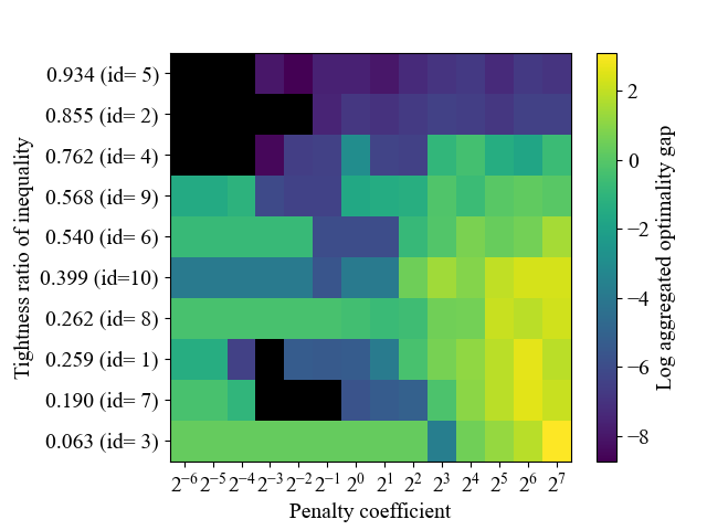
(a) $n=100,d=25$

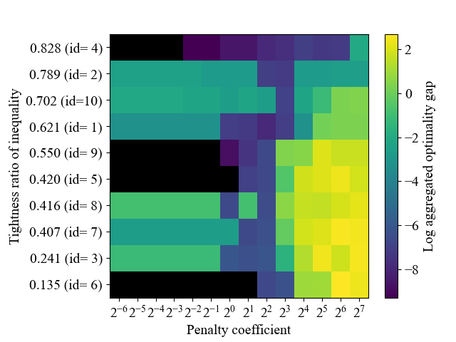
(b) $n=100,d=50$

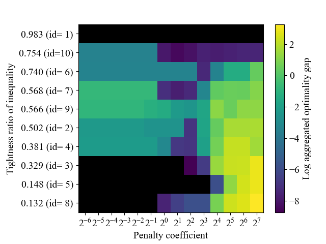
(c) $n=100,d=75$

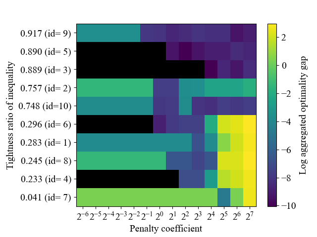
(d) $n=100,d=100$

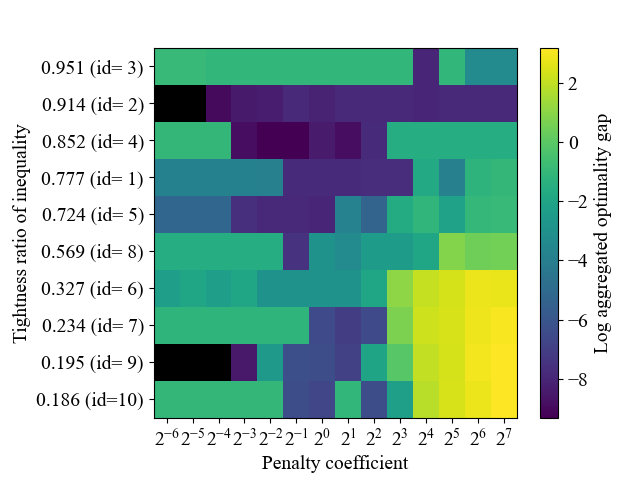
(e) $n=200,d=25$

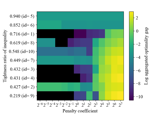
(f) $n=200,d=50$

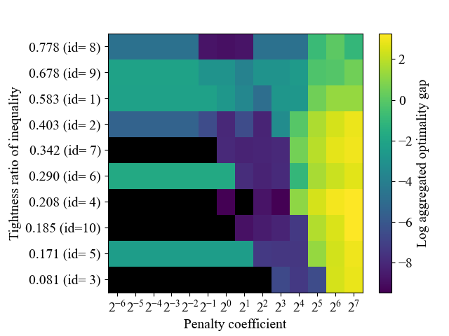
(g) $n=200,d=75$

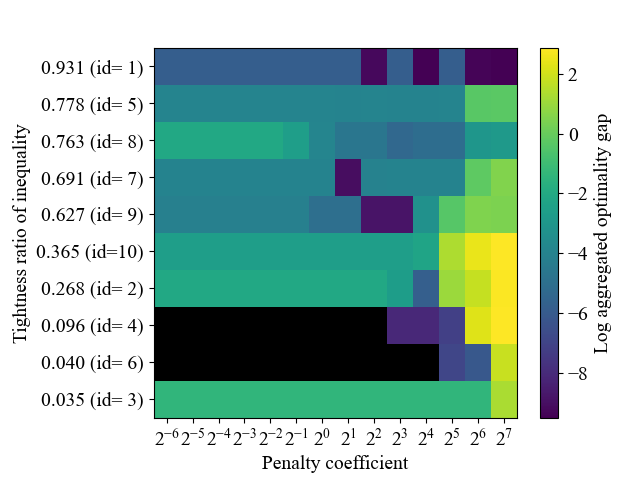
(h) $n=200,d=100$

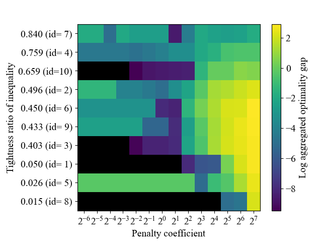
(i) $n=300,d=25$

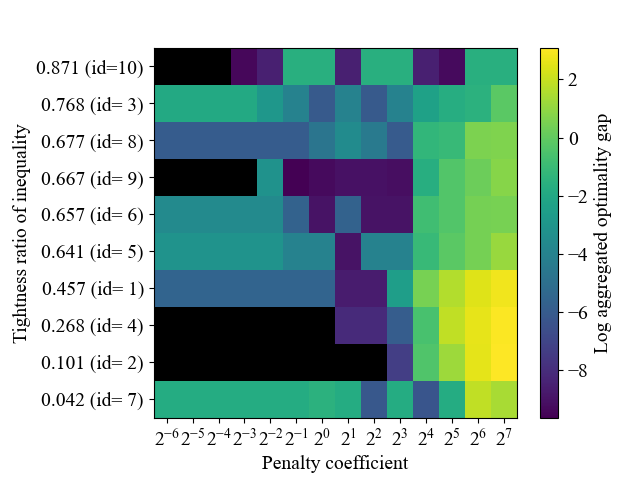
(j) $n=300,d=50$

Figure 6: Aggregated optimality gap for SA-RI on all 100 medium-sized QKP instances. Color bar for gap is shown in log scale. Zero gap (i.e. 100% success rate) is shown in black. Instances are sorted with tightness ratio $\alpha=C/\sum_{i}w_{i}$ for each combination of problem size $n$ and density $d$.

TABLE XIII: Full Results of Ising Machine on Medium-sized Instances.

Instance		Gurobi			AE							AE-R						AE-I						AE-RI
$n$_$d$_id	Optimal	Score	Gap		$a$	FS	Mean	Best	Gap	SR		$a$	Mean	Best	Gap	SR		$a$	Mean	Best	Gap	SR		$a$	Mean	Best	Gap	SR
100_25_1	18558	18558	0.000		5	1.0	18557.70	18558	0.000	0.9		5	18557.70	18558	0.000	0.9		3	18558.00	18558	0.000	1.0		3	18558.00	18558	0.000	1.0
100_25_2	56525	56525	0.000		2	1.0	56525.00	56525	0.000	1.0		2	56525.00	56525	0.000	1.0		2	56525.00	56525	0.000	1.0		2	56525.00	56525	0.000	1.0
100_25_3	3752	3752	0.000		10	1.0	3752.00	3752	0.000	1.0		2	3752.00	3752	0.000	1.0		8	3752.00	3752	0.000	1.0		2	3752.00	3752	0.000	1.0
100_25_4	50382	50382	0.000		3	1.0	50382.00	50382	0.000	1.0		3	50382.00	50382	0.000	1.0		3	50382.00	50382	0.000	1.0		3	50382.00	50382	0.000	1.0
100_25_5	61494	61494	0.000		4	1.0	61494.00	61494	0.000	1.0		4	61494.00	61494	0.000	1.0		2	61494.00	61494	0.000	1.0		1	61494.00	61494	0.000	1.0
100_25_6	36360	36360	0.000		6	1.0	36360.00	36360	0.000	1.0		2	36360.00	36360	0.000	1.0		6	36360.00	36360	0.000	1.0		2	36360.00	36360	0.000	1.0
100_25_7	14657	14657	0.000		3	1.0	14657.00	14657	0.000	1.0		3	14657.00	14657	0.000	1.0		2	14657.00	14657	0.000	1.0		1	14657.00	14657	0.000	1.0
100_25_8	20452	20452	0.000		3	1.0	20452.00	20452	0.000	1.0		3	20452.00	20452	0.000	1.0		3	20452.00	20452	0.000	1.0		3	20452.00	20452	0.000	1.0
100_25_9	35438	35438	0.000		5	1.0	35438.00	35438	0.000	1.0		5	35438.00	35438	0.000	1.0		5	35438.00	35438	0.000	1.0		5	35438.00	35438	0.000	1.0
100_25_10	24930	24930	0.000		3	1.0	24930.00	24930	0.000	1.0		3	24930.00	24930	0.000	1.0		3	24930.00	24930	0.000	1.0		3	24930.00	24930	0.000	1.0
100_50_1	83742	83742	0.000		3	1.0	83742.00	83742	0.000	1.0		3	83742.00	83742	0.000	1.0		3	83742.00	83742	0.000	1.0		2	83742.00	83742	0.000	1.0
100_50_2	104856	104856	0.000		3	1.0	104856.00	104856	0.000	1.0		3	104856.00	104856	0.000	1.0		3	104856.00	104856	0.000	1.0		3	104856.00	104856	0.000	1.0
100_50_3	34006	34006	0.000		4	1.0	34006.00	34006	0.000	1.0		4	34006.00	34006	0.000	1.0		4	34006.00	34006	0.000	1.0		3	34006.00	34006	0.000	1.0
100_50_4	105996	105996	0.000		2	1.0	105996.00	105996	0.000	1.0		2	105996.00	105996	0.000	1.0		2	105996.00	105996	0.000	1.0		1	105996.00	105996	0.000	1.0
100_50_5	56464	56464	0.000		4	1.0	56464.00	56464	0.000	1.0		4	56464.00	56464	0.000	1.0		3	56464.00	56464	0.000	1.0		3	56464.00	56464	0.000	1.0
100_50_6	16083	16083	0.000		2	1.0	16083.00	16083	0.000	1.0		2	16083.00	16083	0.000	1.0		2	16083.00	16083	0.000	1.0		1	16083.00	16083	0.000	1.0
100_50_7	52819	52819	0.000		2	1.0	52819.00	52819	0.000	1.0		2	52819.00	52819	0.000	1.0		2	52819.00	52819	0.000	1.0		2	52819.00	52819	0.000	1.0
100_50_8	54246	54246	0.000		4	1.0	54246.00	54246	0.000	1.0		4	54246.00	54246	0.000	1.0		4	54246.00	54246	0.000	1.0		4	54246.00	54246	0.000	1.0
100_50_9	68974	68974	0.000		3	1.0	68974.00	68974	0.000	1.0		3	68974.00	68974	0.000	1.0		3	68974.00	68974	0.000	1.0		2	68974.00	68974	0.000	1.0
100_50_10	88634	88634	0.000		9	1.0	88607.00	88634	0.000	0.5		9	88607.00	88634	0.000	0.5		8	88613.70	88634	0.000	0.7		8	88613.70	88634	0.000	0.7
100_75_1	189137	189137	0.000		3	1.0	189089.00	189137	0.000	0.9		1	189137.00	189137	0.000	1.0		3	189137.00	189137	0.000	1.0		1	189137.00	189137	0.000	1.0
100_75_2	95074	95074	0.000		4	1.0	95032.90	95074	0.000	0.5		4	95032.90	95074	0.000	0.5		5	95064.80	95074	0.000	0.8		5	95064.80	95074	0.000	0.8
100_75_3	62098	62098	0.000		2	1.0	62098.00	62098	0.000	1.0		2	62098.00	62098	0.000	1.0		2	62098.00	62098	0.000	1.0		1	62098.00	62098	0.000	1.0
100_75_4	72245	72245	0.000		7	1.0	72232.20	72245	0.000	0.5		7	72232.20	72245	0.000	0.5		9	72244.50	72245	0.000	0.9		9	72244.50	72245	0.000	0.9
100_75_5	27616	27616	0.000		3	1.0	27616.00	27616	0.000	1.0		1	27616.00	27616	0.000	1.0		2	27616.00	27616	0.000	1.0		1	27616.00	27616	0.000	1.0
100_75_6	145273	145273	0.000		2	1.0	145273.00	145273	0.000	1.0		2	145273.00	145273	0.000	1.0		2	145273.00	145273	0.000	1.0		2	145273.00	145273	0.000	1.0
100_75_7	110979	110979	0.000		6	1.0	110960.70	110979	0.000	0.5		6	110960.70	110979	0.000	0.5		7	110977.20	110979	0.000	0.8		7	110977.20	110979	0.000	0.8
100_75_8	19570	19570	0.000		2	1.0	19570.00	19570	0.000	1.0		2	19570.00	19570	0.000	1.0		2	19570.00	19570	0.000	1.0		1	19570.00	19570	0.000	1.0
100_75_9	104341	104341	0.000		8	1.0	104262.50	104341	0.000	0.3		8	104262.50	104341	0.000	0.3		6	104328.10	104341	0.000	0.8		6	104328.10	104341	0.000	0.8
100_75_10	143740	143740	0.000		8	1.0	143702.40	143740	0.000	0.7		8	143702.40	143740	0.000	0.7		6	143740.00	143740	0.000	1.0		1	143740.00	143740	0.000	1.0
100_100_1	81978	81978	0.000		5	1.0	81978.00	81978	0.000	1.0		5	81978.00	81978	0.000	1.0		5	81978.00	81978	0.000	1.0		5	81978.00	81978	0.000	1.0
100_100_2	190424	190424	0.000		4	1.0	190410.40	190424	0.000	0.8		4	190410.40	190424	0.000	0.8		4	190416.20	190424	0.000	0.8		4	190416.20	190424	0.000	0.8
100_100_3	225434	225434	0.000		3	1.0	225412.40	225434	0.000	0.7		3	225412.40	225434	0.000	0.7		3	225434.00	225434	0.000	1.0		2	225434.00	225434	0.000	1.0
100_100_4	63028	63028	0.000		3	1.0	63028.00	63028	0.000	1.0		3	63028.00	63028	0.000	1.0		3	63028.00	63028	0.000	1.0		1	63028.00	63028	0.000	1.0
100_100_5	230076	230076	0.000		3	1.0	229861.00	230076	0.000	0.7		3	229861.00	230076	0.000	0.7		3	230076.00	230076	0.000	1.0		1	230076.00	230076	0.000	1.0
100_100_6	74358	74358	0.000		3	1.0	74358.00	74358	0.000	1.0		3	74358.00	74358	0.000	1.0		3	74358.00	74358	0.000	1.0		3	74358.00	74358	0.000	1.0
100_100_7	10330	10330	0.000		4	1.0	10330.00	10330	0.000	1.0		4	10330.00	10330	0.000	1.0		4	10330.00	10330	0.000	1.0		4	10330.00	10330	0.000	1.0
100_100_8	62582	62582	0.000		3	1.0	62582.00	62582	0.000	1.0		3	62582.00	62582	0.000	1.0		3	62582.00	62582	0.000	1.0		1	62582.00	62582	0.000	1.0
100_100_9	232754	232754	0.000		7	1.0	232270.00	232754	0.000	0.2		7	232270.00	232754	0.000	0.2		4	232754.00	232754	0.000	1.0		2	232754.00	232754	0.000	1.0
100_100_10	193262	193262	0.000		7	1.0	193246.10	193262	0.000	0.7		7	193246.10	193262	0.000	0.7		4	193262.00	193262	0.000	1.0		2	193262.00	193262	0.000	1.0
200_25_1	204441	204441	0.000		5	1.0	200560.60	204401	0.020	0.0		5	204006.70	204401	0.020	0.0		7	204351.60	204441	0.000	0.4		7	204397.30	204441	0.000	0.7
200_25_2	239573	239573	0.000		10	1.0	237686.30	239573	0.000	0.1		3	239511.70	239573	0.000	0.2		10	239568.50	239573	0.000	0.7		3	239570.00	239573	0.000	0.8
200_25_3	245463	245463	0.000		8	1.0	242063.30	245463	0.000	0.3		8	242063.30	245463	0.000	0.3		9	245338.30	245463	0.000	0.4		6	245119.50	245463	0.000	0.5
200_25_4	222361	222361	0.000		6	1.0	220185.30	222361	0.000	0.3		4	222134.60	222361	0.000	0.8		6	222323.90	222361	0.000	0.8		6	222361.00	222361	0.000	1.0
200_25_5	187324	187324	0.000		8	1.0	186980.30	187316	4.3E-3	0.0		4	187130.00	187324	0.000	0.1		7	187310.80	187324	0.000	0.3		5	187318.10	187324	0.000	0.3
200_25_6	80351	80351	0.000		5	1.0	80227.90	80351	0.000	0.5		5	80271.00	80351	0.000	0.5		5	80309.10	80351	0.000	0.5		5	80312.90	80351	0.000	0.5
200_25_7	59036	59036	0.000		7	1.0	59029.20	59036	0.000	0.8		7	59029.20	59036	0.000	0.8		9	59036.00	59036	0.000	1.0		9	59036.00	59036	0.000	1.0
200_25_8	149433	149433	0.000		9	1.0	149152.30	149407	0.017	0.0		9	149152.30	149407	0.017	0.0		8	149394.10	149433	0.000	0.4		8	149394.10	149433	0.000	0.4
200_25_9	49366	49366	0.000		7	1.0	49363.20	49366	0.000	0.8		7	49363.20	49366	0.000	0.8		7	49366.00	49366	0.000	1.0		7	49366.00	49366	0.000	1.0
200_25_10	48459	48459	0.000		4	1.0	48459.00	48459	0.000	1.0		4	48459.00	48459	0.000	1.0		4	48459.00	48459	0.000	1.0		4	48459.00	48459	0.000	1.0

TABLE XIII: Full Results of Ising Machine on Medium-sized Instances (continued).

Instance		Gurobi			AE							AE-R						AE-I						AE-RI
$n$_$d$_id	Optimal	Score	Gap		$a$	FS	Mean	Best	Gap	SR		$a$	Mean	Best	Gap	SR		$a$	Mean	Best	Gap	SR		$a$	Mean	Best	Gap	SR
200_50_1	372097	372097	0.000		4	1.0	372097.00	372097	0.000	1.0		3	372097.00	372097	0.000	1.0		4	372097.00	372097	0.000	1.0		2	372097.00	372097	0.000	1.0
200_50_2	211130	211130	0.000		4	0.6	203100.17	211122	3.8E-3	0.0		4	210236.80	211122	3.8E-3	0.0		10	210992.40	211130	0.000	0.1		3	211052.50	211130	0.000	0.1
200_50_3	227185	227185	0.000		9	1.0	226925.00	227185	0.000	0.1		9	226925.00	227185	0.000	0.1		6	227167.10	227185	0.000	0.9		1	227185.00	227185	0.000	1.0
200_50_4	228572	228572	0.000		4	1.0	228572.00	228572	0.000	1.0		4	228572.00	228572	0.000	1.0		4	228572.00	228572	0.000	1.0		3	228572.00	228572	0.000	1.0
200_50_5	479651	479651	0.000		9	1.0	477806.20	479651	0.000	0.4		9	477806.20	479651	0.000	0.4		9	479548.30	479651	0.000	0.5		3	479551.00	479651	0.000	0.5
200_50_6	426777	426672	0.025		8	1.0	424845.00	426777	0.000	0.1		8	424845.00	426777	0.000	0.1		7	426750.20	426777	0.000	0.7		7	426757.10	426777	0.000	0.7
200_50_7	220890	220890	0.000		6	1.0	220720.90	220890	0.000	0.2		6	220720.90	220890	0.000	0.2		6	220841.30	220890	0.000	0.3		1	220868.40	220890	0.000	0.7
200_50_8	317952	317952	0.000		5	1.0	317803.90	317952	0.000	0.2		5	317803.90	317952	0.000	0.2		5	317913.90	317952	0.000	0.7		2	317952.00	317952	0.000	1.0
200_50_9	104936	104936	0.000		5	1.0	104742.10	104936	0.000	0.1		5	104742.10	104936	0.000	0.1		6	104884.90	104936	0.000	0.9		3	104904.60	104936	0.000	0.9
200_50_10	284751	284751	0.000		5	1.0	284299.40	284745	2.1E-3	0.0		5	284299.40	284745	2.1E-3	0.0		5	284632.00	284751	0.000	0.2		5	284635.70	284751	0.000	0.3
200_75_1	442894	442894	0.000		10	1.0	441907.10	442672	0.050	0.0		10	441907.10	442672	0.050	0.0		10	442719.90	442894	0.000	0.3		3	442752.70	442894	0.000	0.5
200_75_2	286643	286643	0.000		5	1.0	286572.50	286643	0.000	0.2		5	286572.50	286643	0.000	0.2		5	286630.60	286643	0.000	0.6		5	286630.90	286643	0.000	0.6
200_75_3	61924	61924	0.000		10	1.0	61924.00	61924	0.000	1.0		10	61924.00	61924	0.000	1.0		7	61924.00	61924	0.000	1.0		1	61924.00	61924	0.000	1.0
200_75_4	128351	128351	0.000		3	1.0	128351.00	128351	0.000	1.0		3	128351.00	128351	0.000	1.0		3	128351.00	128351	0.000	1.0		1	128351.00	128351	0.000	1.0
200_75_5	137885	137885	0.000		9	1.0	137842.90	137885	0.000	0.7		9	137842.90	137885	0.000	0.7		5	137885.00	137885	0.000	1.0		5	137885.00	137885	0.000	1.0
200_75_6	229631	229631	0.000		7	1.0	228703.10	229631	0.000	0.1		7	228703.10	229631	0.000	0.1		6	229159.00	229631	0.000	0.3		3	229592.90	229631	0.000	0.9
200_75_7	269887	269887	0.000		5	1.0	269846.60	269887	0.000	0.6		5	269846.60	269887	0.000	0.6		6	269863.10	269887	0.000	0.9		6	269863.10	269887	0.000	0.9
200_75_8	600858	600858	0.000		5	0.7	592861.00	600819	6.5E-3	0.0		5	600507.50	600858	0.000	0.4		7	600155.90	600858	0.000	0.3		5	600858.00	600858	0.000	1.0
200_75_9	516771	516771	0.000		10	1.0	516262.00	516619	0.029	0.0		10	516262.00	516619	0.029	0.0		8	516714.90	516771	0.000	0.5		8	516714.90	516771	0.000	0.5
200_75_10	142694	142694	0.000		6	1.0	142683.60	142694	0.000	0.9		6	142683.60	142694	0.000	0.9		4	142694.00	142694	0.000	1.0		1	142694.00	142694	0.000	1.0
200_100_1	937149	937149	0.000		10	1.0	932240.80	936716	0.046	0.0		4	936329.60	936742	0.043	0.0		10	937143.80	937149	0.000	0.8		9	937146.40	937149	0.000	0.9
200_100_2	303058	303058	0.000		10	1.0	302835.40	303058	0.000	0.2		10	302835.40	303058	0.000	0.2		10	303019.90	303058	0.000	0.6		10	303019.90	303058	0.000	0.6
200_100_3	29367	29367	0.000		4	1.0	29367.00	29367	0.000	1.0		4	29367.00	29367	0.000	1.0		4	29367.00	29367	0.000	1.0		4	29367.00	29367	0.000	1.0
200_100_4	100838	100838	0.000		4	1.0	100838.00	100838	0.000	1.0		4	100838.00	100838	0.000	1.0		3	100838.00	100838	0.000	1.0		1	100838.00	100838	0.000	1.0
200_100_5	786635	786635	0.000		6	1.0	786527.90	786635	0.000	0.1		3	786516.60	786635	0.000	0.5		5	786604.80	786635	0.000	0.8		6	786605.20	786635	0.000	0.8
200_100_6	41171	41171	0.000		3	1.0	41171.00	41171	0.000	1.0		3	41171.00	41171	0.000	1.0		3	41171.00	41171	0.000	1.0		1	41171.00	41171	0.000	1.0
200_100_7	701094	701094	0.000		9	1.0	700500.00	701094	0.000	0.1		9	700500.00	701094	0.000	0.1		7	701088.50	701094	0.000	0.9		9	701088.50	701094	0.000	0.9
200_100_8	782443	782443	0.000		10	1.0	781342.10	782201	0.031	0.0		10	781342.10	782201	0.031	0.0		9	782403.30	782443	0.000	0.3		3	782356.30	782443	0.000	0.4
200_100_9	628992	628992	0.000		6	1.0	627248.30	628948	7.0E-3	0.0		6	627248.30	628948	7.0E-3	0.0		4	628932.40	628992	0.000	0.5		4	628974.90	628992	0.000	0.5
200_100_10	378442	378442	0.000		8	1.0	378240.50	378442	0.000	0.1		8	378240.50	378442	0.000	0.1		7	378442.00	378442	0.000	1.0		7	378442.00	378442	0.000	1.0
300_25_1	29140	29140	0.000		9	1.0	29129.20	29140	0.000	0.5		9	29129.20	29140	0.000	0.5		9	29140.00	29140	0.000	1.0		2	29140.00	29140	0.000	1.0
300_25_2	281990	281990	0.000		10	1.0	281559.20	281990	0.000	0.1		10	281559.20	281990	0.000	0.1		8	281832.50	281990	0.000	0.2		6	281960.30	281990	0.000	0.3
300_25_3	231075	231075	0.000		9	1.0	230378.60	230873	0.087	0.0		4	231075.00	231075	0.000	1.0		8	230863.20	231075	0.000	0.3		1	231075.00	231075	0.000	1.0
300_25_4	444759	444759	0.000		9	1.0	430978.60	444247	0.115	0.0		2	444401.60	444725	7.6E-3	0.0		5	444430.00	444759	0.000	0.1		5	444709.30	444759	0.000	0.3
300_25_5	14988	14988	0.000		9	1.0	14988.00	14988	0.000	1.0		4	14988.00	14988	0.000	1.0		9	14988.00	14988	0.000	1.0		4	14988.00	14988	0.000	1.0
300_25_6	269782	269782	0.000		10	1.0	268277.20	269601	0.067	0.0		2	269536.10	269782	0.000	0.9		8	269272.67	269782	0.000	0.1		2	269770.90	269782	0.000	0.9
300_25_7	485263	485263	0.000		8	0.9	479607.22	484736	0.109	0.0		6	484404.90	485004	0.053	0.0		4	485143.38	485263	0.000	0.1		4	485125.60	485263	0.000	0.1
300_25_8	9343	9343	0.000		10	1.0	9343.00	9343	0.000	1.0		10	9343.00	9343	0.000	1.0		9	9343.00	9343	0.000	1.0		1	9343.00	9343	0.000	1.0
300_25_9	250761	250761	0.000		9	1.0	250555.80	250751	4.0E-3	0.0		9	250555.80	250751	4.0E-3	0.0		9	250695.10	250761	0.000	0.2		7	250755.00	250761	0.000	0.4
300_25_10	383377	383377	0.000		8	1.0	382810.20	383377	0.000	0.1		4	383377.00	383377	0.000	1.0		7	383263.50	383377	0.000	0.3		1	383377.00	383377	0.000	1.0
300_50_1	513379	513379	0.000		10	1.0	513018.60	513379	0.000	0.2		10	513018.60	513379	0.000	0.2		10	513353.00	513379	0.000	0.7		5	513372.30	513379	0.000	0.9
300_50_2	105543	105543	0.000		6	1.0	105523.80	105543	0.000	0.9		4	105543.00	105543	0.000	1.0		6	105543.00	105543	0.000	1.0		3	105543.00	105543	0.000	1.0
300_50_3	875788	875788	0.000		10	1.0	873068.30	874564	0.140	0.0		4	873757.50	875788	0.000	0.2		6	874591.60	875769	2.2E-3	0.0		5	875684.50	875788	0.000	0.3
300_50_4	307124	307124	0.000		10	1.0	306912.10	307124	0.000	0.1		4	305157.30	307124	0.000	0.2		9	307079.70	307124	0.000	0.5		7	307123.30	307124	0.000	0.9
300_50_5	727820	727820	0.000		9	1.0	727446.60	727820	0.000	0.1		5	727441.60	727820	0.000	0.2		10	727779.20	727820	0.000	0.7		10	727779.20	727820	0.000	0.7
300_50_6	734053	734053	0.000		8	1.0	730756.60	734053	0.000	0.1		5	733876.80	734053	0.000	0.3		8	732651.30	734053	0.000	0.2		5	734048.20	734053	0.000	0.8
300_50_7	43595	43595	0.000		8	1.0	43558.60	43595	0.000	0.2		8	43558.60	43595	0.000	0.2		4	43570.90	43595	0.000	0.6		4	43571.80	43595	0.000	0.6
300_50_8	767977	767977	0.000		8	1.0	767291.40	767937	5.2E-3	0.0		4	767869.30	767948	3.8E-3	0.0		10	767834.40	767977	0.000	0.1		3	767952.80	767977	0.000	0.4
300_50_9	761351	761351	0.000		7	0.6	732640.67	761007	0.045	0.0		4	761153.00	761351	0.000	0.2		10	760476.40	761351	0.000	0.1		2	761351.00	761351	0.000	1.0
300_50_10	996070	996070	0.000		7	1.0	977326.60	993922	0.216	0.0		5	994350.00	996069	1.0E-4	0.0		7	995135.60	996070	0.000	0.4		1	995605.10	996070	0.000	0.8

TABLE XIV: Full Results of Ising Machine on Large Instances (Greedy, AE, and AE-I).

Instance		Greedy			AE							AE-I
$n$_$d$_id	Best-known	Score	Gap		$a$	FS	Mean	Best	Gap	SR		$a$	FS	Mean	Best	Gap	SR
1000_25_1	6172407	6165313	0.115		8	1.0	6046565.20	6143481	0.469	0.0		7	1.0	6168157.90	6172407	0.000	0.1
1000_25_2	229941	229941	0.000		9	0.1	227137.00	227137	1.219	0.0		9	0.1	229057.00	229057	0.384	0.0
1000_25_3	172418	172362	0.032		8	0.1	118485.00	118485	31.280	0.0		8	0.1	137516.00	137516	20.243	0.0
1000_25_4	367426	367426	0.000		-	0	-	-	-	-		-	0	-	-	-	-
1000_25_5	4885611	4884016	0.033		18	1.0	4794876.00	4865871	0.404	0.0		7	0.9	4882635.56	4885573	7.8E-4	0.0
1000_25_6	15689	15689	0.000		9	1.0	15689.00	15689	0.000	1.0		9	1.0	15689.00	15689	0.000	1.0
1000_25_7	4945810	4943898	0.039		5	0.9	4877049.44	4908591	0.753	0.0		4	0.9	4944271.78	4945810	0.000	0.1
1000_25_8	1710198	1709986	0.012		-	0	-	-	-	-		-	0	-	-	-	-
1000_25_9	496315	496315	0.000		-	0	-	-	-	-		-	0	-	-	-	-
1000_25_10	1173792	1173627	0.014		-	0	-	-	-	-		-	0	-	-	-	-
1000_50_1	5663590	5663518	1.3E-3		-	0	-	-	-	-		-	0	-	-	-	-
1000_50_2	180831	180725	0.059		6	0.1	178358.00	178358	1.368	0.0		6	0.1	180220.00	180220	0.338	0.0
1000_50_3	11384283	11384182	8.9E-4		8	1.0	10942873.80	11304391	0.702	0.0		3	1.0	11384044.80	11384283	0.000	0.1
1000_50_4	322226	322170	0.017		9	0.1	314771.00	314771	2.314	0.0		9	0.1	320179.00	320179	0.635	0.0
1000_50_5	9984247	9983024	0.012		13	1.0	9756809.50	9932876	0.515	0.0		4	0.8	9981206.50	9984002	2.5E-3	0.0
1000_50_6	4106261	4105256	0.024		-	0	-	-	-	-		-	0	-	-	-	-
1000_50_7	10498370	10497911	4.4E-3		5	1.0	10293633.60	10426694	0.683	0.0		2	0.9	10497958.56	10498370	0.000	0.1
1000_50_8	4981146	4978776	0.048		17	0.1	4858893.00	4858893	2.454	0.0		13	0.1	4978216.00	4978216	0.059	0.0
1000_50_9	1727861	1727861	0.000		10	0.1	1654507.00	1654507	4.245	0.0		10	0.1	1682796.00	1682796	2.608	0.0
1000_50_10	2340724	2340115	0.026		18	0.1	2332302.00	2332302	0.360	0.0		18	0.1	2336272.00	2336272	0.190	0.0
1000_75_1	11570056	11568107	0.017		14	0.7	11434541.71	11489586	0.696	0.0		17	0.8	11521261.50	11569868	1.6E-3	0.0
1000_75_2	1901389	1901083	0.016		-	0	-	-	-	-		-	0	-	-	-	-
1000_75_3	2096485	2090674	0.277		19	0.3	1991055.00	2086915	0.456	0.0		20	0.3	2084592.33	2091367	0.244	0.0
1000_75_4	7305321	7305320	1.4E-5		-	0	-	-	-	-		-	0	-	-	-	-
1000_75_5	13970842	13967977	0.021		16	1.0	13730507.30	13900932	0.500	0.0		8	1.0	13968979.30	13969760	7.7E-3	0.0
1000_75_6	12288738	12287677	8.6E-3		10	1.0	12106698.20	12171993	0.950	0.0		10	1.0	12285291.60	12288736	1.6E-5	0.0
1000_75_7	1095837	1093066	0.253		10	0.1	528554.00	528554	51.767	0.0		10	0.1	579407.00	579407	47.127	0.0
1000_75_8	5575813	5571863	0.071		-	0	-	-	-	-		-	0	-	-	-	-
1000_75_9	695774	695060	0.103		10	0.1	692459.00	692459	0.476	0.0		10	0.1	694689.00	694689	0.156	0.0
1000_75_10	2507677	2507415	0.010		-	0	-	-	-	-		-	0	-	-	-	-
1000_100_1	6243494	6240386	0.050		20	0.1	6237741.00	6237741	0.092	0.0		20	0.1	6241605.00	6241605	0.030	0.0
1000_100_2	4854086	4851219	0.059		19	0.2	4026639.50	4740591	2.338	0.0		19	0.2	4808609.50	4851243	0.059	0.0
1000_100_3	3172022	3169717	0.073		-	0	-	-	-	-		-	0	-	-	-	-
1000_100_4	754727	754041	0.091		20	1.0	753275.30	754048	0.090	0.0		20	1.0	754459.30	754663	8.5E-3	0.0
1000_100_5	18646620	18644356	0.012		19	1.0	18411742.00	18553784	0.498	0.0		18	1.0	18612884.10	18646307	1.7E-3	0.0
1000_100_6	16020232	16019071	7.2E-3		10	0.5	15832101.20	15900553	0.747	0.0		8	0.6	16004784.50	16019644	3.7E-3	0.0
1000_100_7	12936205	12935892	2.4E-3		-	0	-	-	-	-		-	0	-	-	-	-
1000_100_8	6927738	6927088	9.4E-3		-	0	-	-	-	-		-	0	-	-	-	-
1000_100_9	3874959	3874666	7.6E-3		-	0	-	-	-	-		-	0	-	-	-	-
1000_100_10	1334494	1333599	0.067		20	0.8	1331945.25	1332813	0.126	0.0		20	0.8	1333752.88	1334390	7.8E-3	0.0
2000_25_1	5268188	5268172	3.0E-4		19	0.1	4264680.00	4264680	19.048	0.0		19	0.1	5264179.00	5264179	0.076	0.0
2000_25_2	13294030	13292220	0.014		18	0.6	13197215.00	13238963	0.414	0.0		12	0.1	13293975.00	13293975	4.1E-4	0.0
2000_25_3	5500433	5499695	0.013		19	0.1	3862911.00	3862911	29.771	0.0		19	0.1	5492238.00	5492238	0.149	0.0
2000_25_4	14625118	14624957	1.1E-3		20	0.9	14438872.67	14558124	0.458	0.0		10	0.7	14621883.71	14625118	0.000	0.1
2000_25_5	5975751	5974429	0.022		-	0	-	-	-	-		-	0	-	-	-	-
2000_25_6	4491691	4491649	9.4E-4		-	0	-	-	-	-		-	0	-	-	-	-
2000_25_7	6388756	6388705	8.0E-4		20	0.1	5854140.00	5854140	8.368	0.0		20	0.1	6387505.00	6387505	0.020	0.0
2000_25_8	11769873	11767061	0.024		19	0.3	11534726.00	11722386	0.403	0.0		18	0.2	11768276.50	11768330	0.013	0.0
2000_25_9	10960328	10960313	1.4E-4		19	0.2	10577342.50	10900905	0.542	0.0		8	0.1	10960113.00	10960113	2.0E-3	0.0
2000_25_10	139236	139236	0.000		16	0.1	3945.00	3945	97.167	0.0		16	0.1	55528.00	55528	60.120	0.0
2000_50_1	7070736	7064882	0.083		-	0	-	-	-	-		-	0	-	-	-	-
2000_50_2	12587545	12587266	2.2E-3		11	0.1	12276905.00	12276905	2.468	0.0		12	0.1	12585105.00	12585105	0.019	0.0
2000_50_3	27268336	27268336	0.000		20	0.7	26632622.14	27148430	0.440	0.0		11	0.2	27267716.50	27268037	1.1E-3	0.0
2000_50_4	17754434	17752803	9.2E-3		15	0.3	15946463.67	17665973	0.498	0.0		15	0.3	17750698.00	17752976	8.2E-3	0.0
2000_50_5	16806059	16803639	0.014		15	0.1	16161265.00	16161265	3.837	0.0		12	0.1	16802163.00	16802163	0.023	0.0
2000_50_6	23076155	23074597	6.8E-3		17	0.3	22841543.00	22867634	0.904	0.0		17	0.3	23062541.67	23074825	5.8E-3	0.0
2000_50_7	28759759	28756239	0.012		9	0.2	28600532.50	28600679	0.553	0.0		8	0.2	28756905.00	28757496	7.9E-3	0.0
2000_50_8	1580242	1580242	0.000		16	0.1	1206100.00	1206100	23.676	0.0		16	0.1	1282894.00	1282894	18.817	0.0
2000_50_9	26523791	26523221	2.1E-3		9	0.4	25837132.25	26348755	0.660	0.0		11	0.4	26521898.00	26523328	1.7E-3	0.0
2000_50_10	24747047	24747047	0.000		20	0.2	24559204.00	24630282	0.472	0.0		10	0.1	24746954.00	24746954	3.8E-4	0.0
2000_75_1	25121998	25119968	8.1E-3		17	0.1	24941261.00	24941261	0.719	0.0		13	0.2	25094179.50	25119908	8.3E-3	0.0
2000_75_2	12664670	12664008	5.2E-3		-	0	-	-	-	-		-	0	-	-	-	-
2000_75_3	43943994	43941916	4.7E-3		19	0.5	43299897.20	43678829	0.603	0.0		8	0.2	43943590.00	43943703	6.6E-4	0.0
2000_75_4	37496613	37496099	1.4E-3		20	0.4	33300362.50	37331383	0.441	0.0		9	0.1	37496271.00	37496271	9.1E-4	0.0
2000_75_5	24835349	24833545	7.3E-3		17	0.2	20223954.50	22728621	8.483	0.0		13	0.1	24832245.00	24832245	0.012	0.0
2000_75_6	45137758	45137758	0.000		10	0.4	44662139.25	44868910	0.596	0.0		5	0.2	45137345.00	45137758	0.000	0.1
2000_75_7	25502608	25502409	7.8E-4		15	0.1	24935633.00	24935633	2.223	0.0		18	0.1	25478168.00	25478168	0.096	0.0
2000_75_8	10067892	10067546	3.4E-3		-	0	-	-	-	-		-	0	-	-	-	-
2000_75_9	14177079	14169391	0.054		-	0	-	-	-	-		-	0	-	-	-	-
2000_75_10	7815755	7813832	0.025		-	0	-	-	-	-		-	0	-	-	-	-
2000_100_1	37929909	37929771	3.6E-4		17	0.2	35696999.50	37675871	0.670	0.0		8	0.1	37927936.00	37927936	5.2E-3	0.0
2000_100_2	33665281	33639083	0.078		12	0.2	28996903.50	32350573	3.905	0.0		8	0.2	33640008.00	33642902	0.066	0.0
2000_100_3	29952019	29949832	7.3E-3		11	0.1	29346552.00	29346552	2.021	0.0		12	0.1	29948550.00	29948550	0.012	0.0
2000_100_4	26949268	26947203	7.7E-3		15	0.1	26626386.00	26626386	1.198	0.0		14	0.2	26946246.00	26947244	7.5E-3	0.0
2000_100_5	22041715	22038689	0.014		19	0.1	20086249.00	20086249	8.872	0.0		19	0.1	22035826.00	22035826	0.027	0.0
2000_100_6	18868887	18867393	7.9E-3		-	0	-	-	-	-		-	0	-	-	-	-
2000_100_7	15850597	15848026	0.016		-	0	-	-	-	-		-	0	-	-	-	-
2000_100_8	13628967	13628029	6.9E-3		-	0	-	-	-	-		-	0	-	-	-	-
2000_100_9	8394562	8388596	0.071		19	0.1	7097454.00	7097454	15.452	0.0		19	0.1	7249975.00	7249975	13.635	0.0
2000_100_10	4923559	4921159	0.049		18	0.1	3111936.00	3111936	36.795	0.0		15	0.1	3291205.00	3291205	33.154	0.0

TABLE XV: Full Results of Ising Machine on Large Instances (Gurobi, AE-R, and AE-RI).

Instance		Gurobi			AE-R						AE-RI
$n$_$d$_id	Best-known	Score	Gap		$a$	Mean	Best	Gap	SR		$a$	Mean	Best	Gap	SR
1000_25_1	6172407	6172407	0.000		4	6129734.5	6164169	0.133	0.0		7	6168834.5	6172407	0.000	0.2
1000_25_2	229941	229941	0.000		1	228355.2	229902	0.017	0.0		1	229933.5	229941	0.000	0.9
1000_25_3	172418	172418	0.000		6	172418.0	172418	0.000	1.0		6	172418.0	172418	0.000	1.0
1000_25_4	367426	367426	0.000		7	365784.3	367014	0.112	0.0		1	367426.0	367426	0.000	1.0
1000_25_5	4885611	4885611	0.000		6	4884277.2	4885538	1.5E-3	0.0		4	4885138.5	4885611	0.000	0.1
1000_25_6	15689	15689	0.000		5	15689.0	15689	0.000	1.0		1	15689.0	15689	0.000	1.0
1000_25_7	4945810	4945810	0.000		4	4943097.0	4945810	0.000	0.1		4	4945608.4	4945810	0.000	0.3
1000_25_8	1710198	1710132	3.9E-3		7	1709246.1	1710017	0.011	0.0		10	1710007.7	1710198	0.000	0.3
1000_25_9	496315	496315	0.000		6	496304.9	496315	0.000	0.9		5	496315.0	496315	0.000	1.0
1000_25_10	1173792	1173789	2.6E-4		2	1172790.6	1173694	8.3E-3	0.0		10	1173639.3	1173792	0.000	0.1
1000_50_1	5663590	5663590	0.000		6	5663158.6	5663590	0.000	0.1		6	5663574.2	5663590	0.000	0.7
1000_50_2	180831	180831	0.000		10	179702.8	180831	0.000	0.2		5	180831.0	180831	0.000	1.0
1000_50_3	11384283	11384283	0.000		4	11354296.1	11384247	3.2E-4	0.0		5	11384256.1	11384283	0.000	0.7
1000_50_4	322226	322226	0.000		10	320732.0	322222	1.2E-3	0.0		9	322220.4	322226	0.000	0.9
1000_50_5	9984247	9984155	9.2E-4		5	9979380.1	9983164	0.011	0.0		5	9983901.4	9984155	9.2E-4	0.0
1000_50_6	4106261	4106261	0.000		6	4104720.9	4106084	4.3E-3	0.0		4	4106142.3	4106261	0.000	0.8
1000_50_7	10498370	10498370	0.000		6	10485633.4	10498272	9.3E-4	0.0		6	10498331.4	10498370	0.000	0.6
1000_50_8	4981146	4981143	6.0E-5		12	4978197.9	4979892	0.025	0.0		16	4979493.7	4980274	0.018	0.0
1000_50_9	1727861	1727861	0.000		6	1724044.1	1727861	0.000	0.6		6	1727861.0	1727861	0.000	1.0
1000_50_10	2340724	2340724	0.000		16	2339432.1	2340724	0.000	0.1		16	2340023.7	2340724	0.000	0.3
1000_75_1	11570056	11570056	0.000		11	11544807.4	11568936	9.7E-3	0.0		6	11569740.8	11570055	8.6E-6	0.0
1000_75_2	1901389	1901389	0.000		5	1894235.8	1901231	8.3E-3	0.0		10	1899475.3	1901389	0.000	0.5
1000_75_3	2096485	2096485	0.000		16	2093204.3	2096485	0.000	0.1		16	2096471.0	2096485	0.000	0.8
1000_75_4	7305321	7305315	8.2E-5		5	7292449.8	7304592	0.010	0.0		6	7305152.0	7305321	0.000	0.5
1000_75_5	13970842	13970842	0.000		13	13941909.1	13968310	0.018	0.0		10	13969208.3	13969984	6.1E-3	0.0
1000_75_6	12288738	12288738	0.000		6	12287280.1	12288115	5.1E-3	0.0		1	12288438.5	12288738	0.000	0.4
1000_75_7	1095837	1095837	0.000		7	1092604.3	1093131	0.247	0.0		4	1093343.1	1095837	0.000	0.1
1000_75_8	5575813	5575813	0.000		6	5574312.1	5575811	3.6E-5	0.0		15	5575505.5	5575813	0.000	0.4
1000_75_9	695774	695767	1.0E-3		5	694039.0	695064	0.102	0.0		5	695496.2	695774	0.000	0.1
1000_75_10	2507677	2507677	0.000		6	2506795.2	2507677	0.000	0.1		6	2507567.5	2507677	0.000	0.5
1000_100_1	6243494	6243494	0.000		11	6238463.1	6242478	0.016	0.0		11	6243143.8	6243494	0.000	0.1
1000_100_2	4854086	4854086	0.000		14	4851616.1	4852477	0.033	0.0		15	4853764.5	4854043	8.9E-4	0.0
1000_100_3	3172022	3172022	0.000		6	3169655.3	3170376	0.052	0.0		7	3171416.8	3172022	0.000	0.5
1000_100_4	754727	754539	0.025		12	754120.8	754645	0.011	0.0		12	754591.7	754727	0.000	0.2
1000_100_5	18646620	18646607	7.0E-5		11	18601616.7	18643031	0.019	0.0		9	18645693.5	18646535	4.6E-4	0.0
1000_100_6	16020232	16020232	0.000		5	16012775.7	16016672	0.022	0.0		5	16019834.7	16020232	0.000	0.3
1000_100_7	12936205	12936205	0.000		6	12935073.5	12936083	9.4E-4	0.0		5	12928785.2	12936205	0.000	0.4
1000_100_8	6927738	6927671	9.7E-4		6	6925298.8	6925940	0.026	0.0		6	6927168.3	6927606	1.9E-3	0.0
1000_100_9	3874959	3874959	0.000		4	3874196.9	3874959	0.000	0.1		6	3874917.8	3874959	0.000	0.8
1000_100_10	1334494	1334494	0.000		13	1333903.0	1334457	2.8E-3	0.0		11	1334474.0	1334494	0.000	0.5
2000_25_1	5268188	5268188	0.000		8	5267547.6	5268188	0.000	0.2		8	5268171.6	5268188	0.000	0.4
2000_25_2	13294030	13293975	4.1E-4		5	13281482.0	13293956	5.6E-4	0.0		12	13293730.1	13293975	4.1E-4	0.0
2000_25_3	5500433	5500411	4.0E-4		13	5497914.6	5499944	8.9E-3	0.0		7	5499740.7	5500403	5.5E-4	0.0
2000_25_4	14625118	14625031	5.9E-4		13	14620474.6	14624980	9.4E-4	0.0		8	14625069.6	14625118	0.000	0.3
2000_25_5	5975751	5975751	0.000		13	5973488.1	5975675	1.3E-3	0.0		13	5975276.2	5975751	0.000	0.3
2000_25_6	4491691	4491635	1.2E-3		12	4485267.1	4491630	1.4E-3	0.0		10	4491691.0	4491691	0.000	1.0
2000_25_7	6388756	6388756	0.000		13	6388445.2	6388756	0.000	0.2		13	6388744.1	6388756	0.000	0.7
2000_25_8	11769873	11769873	0.000		2	11757436.7	11769873	0.000	0.1		11	11769820.5	11769873	0.000	0.7
2000_25_9	10960328	10960263	5.9E-4		3	10952474.0	10960207	1.1E-3	0.0		11	10960066.9	10960328	0.000	0.1
2000_25_10	139236	139236	0.000		16	138459.9	139236	0.000	0.2		1	139236.0	139236	0.000	1.0
2000_50_1	7070736	7070736	0.000		12	7062808.2	7070341	5.6E-3	0.0		12	7068396.4	7070736	0.000	0.2
2000_50_2	12587545	12587545	0.000		12	12586350.3	12587482	5.0E-4	0.0		12	12587507.0	12587545	0.000	0.7
2000_50_3	27268336	27268336	0.000		3	27268335.2	27268336	0.000	0.9		3	27268336.0	27268336	0.000	1.0
2000_50_4	17754434	17754388	2.6E-4		12	17752283.1	17753673	4.3E-3	0.0		12	17754087.3	17754434	0.000	0.1
2000_50_5	16806059	16805435	3.7E-3		11	16801525.3	16804057	0.012	0.0		12	16804680.5	16805490	3.4E-3	0.0
2000_50_6	23076155	23076097	2.5E-4		12	23074405.9	23075875	1.2E-3	0.0		11	23075852.7	23076155	0.000	0.2
2000_50_7	28759759	28759759	0.000		11	27410959.4	28756657	0.011	0.0		10	28757135.3	28757834	6.7E-3	0.0
2000_50_8	1580242	1580242	0.000		11	1577163.4	1580242	0.000	0.3		1	1580242.0	1580242	0.000	1.0
2000_50_9	26523791	26523791	0.000		8	26519303.3	26523462	1.2E-3	0.0		7	26523472.8	26523791	0.000	0.2
2000_50_10	24747047	24747047	0.000		8	24743522.7	24746936	4.5E-4	0.0		1	24747047.0	24747047	0.000	1.0
2000_75_1	25121998	25121998	0.000		11	25120313.9	25121457	2.2E-3	0.0		11	25121744.4	25121998	0.000	0.4
2000_75_2	12664670	12664670	0.000		11	12656539.5	12664244	3.4E-3	0.0		10	12662072.5	12664670	0.000	0.4
2000_75_3	43943994	43943994	0.000		16	43800921.7	43943366	1.4E-3	0.0		8	43943724.9	43943994	0.000	0.6
2000_75_4	37496613	37496613	0.000		3	37493330.7	37496308	8.1E-4	0.0		2	37496367.3	37496613	0.000	0.2
2000_75_5	24835349	24835349	0.000		11	24828628.7	24831592	0.015	0.0		11	24834632.9	24834948	1.6E-3	0.0
2000_75_6	45137758	45137758	0.000		3	45132276.3	45137758	0.000	0.9		8	45137758.0	45137758	0.000	1.0
2000_75_7	25502608	25502608	0.000		12	25467707.7	25502608	0.000	0.1		4	25495828.7	25502608	0.000	0.3
2000_75_8	10067892	10067892	0.000		11	10064140.4	10067750	1.4E-3	0.0		10	10063814.3	10067892	0.000	0.3
2000_75_9	14177079	14177079	0.000		11	14163838.4	14168633	0.060	0.0		14	14171401.8	14171994	0.036	0.0
2000_75_10	7815755	7815334	5.4E-3		12	7811373.0	7812703	0.039	0.0		20	7814965.3	7815611	1.8E-3	0.0
2000_100_1	37929909	37929909	0.000		4	37926908.4	37929909	0.000	0.1		12	37929518.3	37929909	0.000	0.6
2000_100_2	33665281	33665281	0.000		12	32835326.4	33637892	0.081	0.0		12	33644437.0	33646541	0.056	0.0
2000_100_3	29952019	29951413	2.0E-3		12	29553629.4	29948391	0.012	0.0		10	29951436.0	29952019	0.000	0.1
2000_100_4	26949268	26948616	2.4E-3		13	26943483.1	26947024	8.3E-3	0.0		11	26948996.6	26949268	0.000	0.2
2000_100_5	22041715	22041314	1.8E-3		11	22032284.4	22034438	0.033	0.0		17	22038647.2	22041221	2.2E-3	0.0
2000_100_6	18868887	18868887	0.000		10	18834013.3	18868626	1.4E-3	0.0		10	18866428.5	18868887	0.000	0.2
2000_100_7	15850597	15850597	0.000		10	15847566.7	15848960	0.010	0.0		11	15850259.2	15850594	1.9E-5	0.0
2000_100_8	13628967	13628967	0.000		12	13622163.4	13626547	0.018	0.0		12	13628850.7	13628967	0.000	0.4
2000_100_9	8394562	8394101	5.5E-3		11	8388749.0	8390723	0.046	0.0		20	8394196.6	8394562	0.000	0.4
2000_100_10	4923559	4923387	3.5E-3		13	4918213.2	4919752	0.077	0.0		14	4922601.9	4923470	1.8E-3	0.0

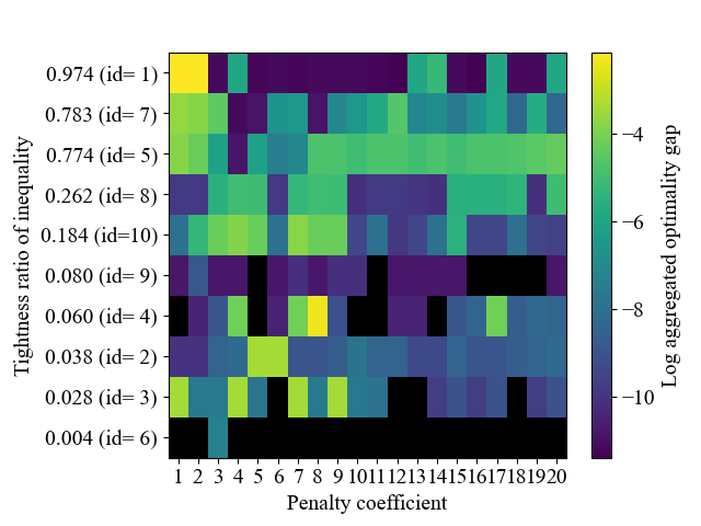
(a) $n=1000,d=25$

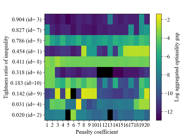
(b) $n=1000,d=50$

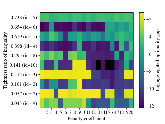
(c) $n=1000,d=75$

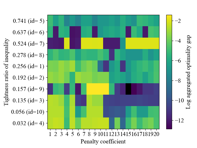
(d) $n=1000,d=100$

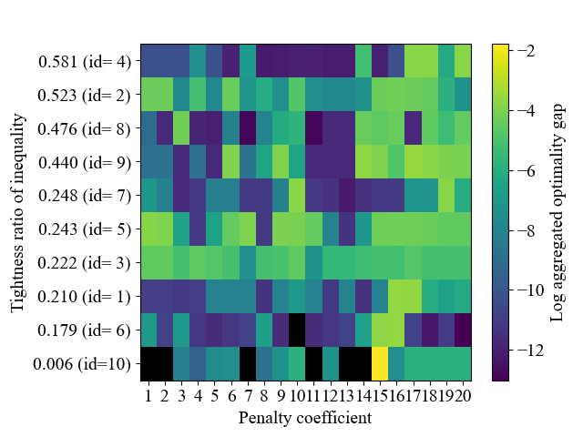
(e) $n=2000,d=25$

(f) $n=2000,d=50$

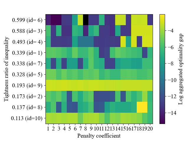
(g) $n=2000,d=75$

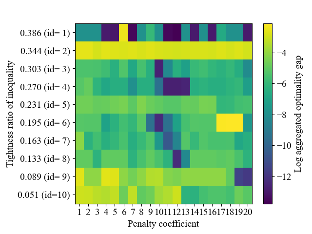
(h) $n=2000,d=100$

Figure 7: Aggregated optimality gap for AE-RI on all 80 large QKP instances. Color bar for gap is shown in log scale. Zero gap (i.e. 100% success rate) is shown in black. Instances are sorted with tightness ratio $\alpha=C/\sum_{i}w_{i}$ for each combination of problem size $n$ and density $d$. Note that penalty coefficient is rescaled and x-axis actually denotes $a$ in Eq. (18). Due to this rescaling, we see less trends in distribution of good penalty coefficient than Fig. 6.

B-B Results on Ising Machine

Full results of the benchmark of AE conducted in Section V are shown in Table XIII, XIV and XV. Legends for columns are the same as those in Table XI except for the optimal penalty coefficient $\lambda$. As we rescaled $\lambda$ as in Eq. (18), the value of $\lambda$ is defined according to the value of $a$ in Eq. (18). Therefore, we report the value of $a$ giving the optimal $\lambda$. Since there are several large instances on which AE cannot obtain feasible a solution even with $a=20$, the results on those instances are not reported.

We also plot the aggregated optimality gap for AE-RI on each instance in Fig. 7. We observe that the tested range of penalty coefficients seems to cover optimal coefficients on most instances. Note that the x-axis corresponds to values of $a$ in Eq. (18), not $\lambda$. Due to the rescaling of $\lambda$, we see less visual trends in Figure 7 compared to Fig. 6. This indicates that the rescaling based on SA analysis also works well when using the Ising machine for large-scale instances.

References

- [1] V. Cacchiani, M. Iori, A. Locatelli, and S. Martello, “Knapsack problems – An overview of recent advances. Part II: Multiple, multidimensional, and quadratic knapsack problems,” Computers & Operations Research, p. 105693, 2022.
- [2] N. Mohseni, P. L. McMahon, and T. Byrnes, “Ising machines as hardware solvers of combinatorial optimization problems,” Nature Reviews Physics, vol. 4, no. 6, pp. 363–379, 2022.
- [3] A. Lucas, “Ising formulations of many NP problems,” Frontiers in physics, p. 5, 2014.
- [4] M. W. Johnson, M. H. Amin, S. Gildert, T. Lanting, F. Hamze, N. Dickson, R. Harris, A. J. Berkley, J. Johansson, P. Bunyk et al., “Quantum annealing with manufactured spins,” Nature, vol. 473, no. 7346, pp. 194–198, 2011.
- [5] A. A. Houck, H. E. Türeci, and J. Koch, “On-chip quantum simulation with superconducting circuits,” Nature Physics, vol. 8, no. 4, pp. 292–299, 2012.
- [6] Z. Wang, A. Marandi, K. Wen, R. L. Byer, and Y. Yamamoto, “Coherent Ising machine based on degenerate optical parametric oscillators,” Physical Review A, vol. 88, no. 6, p. 063853, 2013.
- [7] T. Honjo, T. Sonobe, K. Inaba, T. Inagaki, T. Ikuta, Y. Yamada, T. Kazama, K. Enbutsu, T. Umeki, R. Kasahara et al., “100,000-spin coherent Ising machine,” Science advances, vol. 7, no. 40, p. eabh0952, 2021.
- [8] M. Yamaoka, C. Yoshimura, M. Hayashi, T. Okuyama, H. Aoki, and H. Mizuno, “A 20k-spin Ising chip to solve combinatorial optimization problems with CMOS annealing,” IEEE Journal of Solid-State Circuits, vol. 51, no. 1, pp. 303–309, 2015.
- [9] M. Aramon, G. Rosenberg, E. Valiante, T. Miyazawa, H. Tamura, and H. G. Katzgraber, “Physics-inspired optimization for quadratic unconstrained problems using a digital annealer,” Frontiers in Physics, vol. 7, p. 48, 2019.
- [10] K. Yamamoto, K. Kawamura, K. Ando, N. Mertig, T. Takemoto, M. Yamaoka, H. Teramoto, A. Sakai, S. Takamaeda-Yamazaki, and M. Motomura, “STATICA: A 512-spin 0.25 M-weight annealing processor with an all-spin-updates-at-once architecture for combinatorial optimization with complete spin–spin interactions,” IEEE Journal of Solid-State Circuits, vol. 56, no. 1, pp. 165–178, 2020.
- [11] T. Wang, L. Wu, P. Nobel, and J. Roychowdhury, “Solving combinatorial optimisation problems using oscillator based Ising machines,” Natural Computing, vol. 20, no. 2, pp. 287–306, 2021.
- [12] H. Goto, K. Tatsumura, and A. R. Dixon, “Combinatorial optimization by simulating adiabatic bifurcations in nonlinear Hamiltonian systems,” Science advances, vol. 5, no. 4, p. eaav2372, 2019.
- [13] P. Codognet, D. Diaz, and S. Abreu, “Quantum and digital annealing for the quadratic assignment problem,” in 2022 IEEE International Conference on Quantum Software (QSW). IEEE, 2022, pp. 1–8.
- [14] T. Huang, J. Xu, T. Luo, X. Gu, R. S. M. Goh, and W.-F. Wong, “Benchmarking quantum (-inspired) annealing hardware on practical use cases,” IEEE Transactions on Computers, 2022.
- [15] M. Parizy and N. Togawa, “Analysis and acceleration of the quadratic knapsack problem on an ising machine,” IEICE Transactions on Fundamentals of Electronics, Communications and Computer Sciences, vol. 104, no. 11, pp. 1526–1535, 2021.
- [16] A. Ceselli and M. Premoli, “On good encodings for quantum annealer and digital optimization solvers,” Scientific Reports, vol. 13, no. 1, p. 5628, 2023.
- [17] G. Gallo, P. L. Hammer, and B. Simeone, “Quadratic knapsack problems,” Combinatorial optimization, pp. 132–149, 1980.
- [18] K. Tamura, T. Shirai, H. Katsura, S. Tanaka, and N. Togawa, “Performance comparison of typical binary-integer encodings in an Ising machine,” IEEE Access, vol. 9, pp. 81 032–81 039, 2021.
- [19] S. Jimbo, D. Okonogi, K. Ando, T. Van CHU, J. Yu, M. Motomura, and K. Kawamura, “A hybrid integer encoding method for obtaining high-quality solutions of quadratic knapsack problems on solid-state annealers,” IEICE TRANSACTIONS on Information and Systems, vol. 105, no. 12, pp. 2019–2031, 2022.
- [20] T. Bontekoe, F. Phillipson, and W. v. d. Schoot, “Translating constraints into QUBOs for the quadratic knapsack problem,” in International Conference on Computational Science. Springer, 2023, pp. 90–107.
- [21] K. Yonaga, M. J. Miyama, and M. Ohzeki, “Solving inequality-constrained binary optimization problems on quantum annealer,” arXiv preprint arXiv:2012.06119, 2020.
- [22] Fixstars Corporation, “Fixstars Amplify AE,” 2020. [Online]. Available: https://amplify.fixstars.com/en/engine
- [23] F. D. Fomeni and A. N. Letchford, “A dynamic programming heuristic for the quadratic knapsack problem,” INFORMS Journal on Computing, vol. 26, no. 1, pp. 173–182, 2014.
- [24] Z. Yang, G. Wang, and F. Chu, “An effective GRASP and tabu search for the 0–1 quadratic knapsack problem,” Computers & Operations Research, vol. 40, no. 5, pp. 1176–1185, 2013.
- [25] C. Patvardhan, S. Bansal, and A. Srivastav, “Parallel improved quantum inspired evolutionary algorithm to solve large size quadratic knapsack problems,” Swarm and Evolutionary Computation, vol. 26, pp. 175–190, 2016.
- [26] Y. Chen and J.-K. Hao, “An iterated “hyperplane exploration” approach for the quadratic knapsack problem,” Computers & Operations Research, vol. 77, pp. 226–239, 2017.
- [27] T. Kadowaki and H. Nishimori, “Quantum annealing in the transverse Ising model,” Physical Review E, vol. 58, no. 5, p. 5355, 1998.
- [28] D. Pisinger, “The quadratic knapsack problem—a survey,” Discrete applied mathematics, vol. 155, no. 5, pp. 623–648, 2007.
- [29] A. Billionnet and F. Calmels, “Linear programming for the 0–1 quadratic knapsack problem,” European Journal of Operational Research, vol. 92, no. 2, pp. 310–325, 1996.
- [30] F. Glover, G. Kochenberger, B. Alidaee, and M. Amini, “Solving quadratic knapsack problems by reformulation and tabu search: Single constraint case,” in Combinatorial and global optimization. World Scientific, 2002, pp. 111–121.
- [31] P. C. Chu and J. E. Beasley, “A genetic algorithm for the multidimensional knapsack problem,” Journal of heuristics, vol. 4, no. 1, pp. 63–86, 1998.
- [32] R. Jovanovic and S. Voß, “Solving the quadratic knapsack problem using grasp,” in Metaheuristics for Machine Learning: New Advances and Tools. Springer, 2022, pp. 157–178.
- [33] P. Chaillou, P. Hansen, and Y. Mahieu, “Best network flow bounds for the quadratic knapsack problem,” in Combinatorial Optimization: Lectures given at the 3rd Session of the Centro Internazionale Matematico Estivo (CIME) held at Como, Italy, August 25–September 2, 1986. Springer, 1989, pp. 225–235.
- [34] D. A. Battaglia, G. E. Santoro, and E. Tosatti, “Optimization by quantum annealing: Lessons from hard satisfiability problems,” Physical Review E, vol. 71, no. 6, p. 066707, 2005.
- [35] B. Heim, T. F. Rønnow, S. V. Isakov, and M. Troyer, “Quantum versus classical annealing of Ising spin glasses,” Science, vol. 348, no. 6231, pp. 215–217, 2015.
- [36] A. Billionnet and É. Soutif, “An exact method based on Lagrangian decomposition for the 0–1 quadratic knapsack problem,” European Journal of operational research, vol. 157, no. 3, pp. 565–575, 2004.
- [37] K. Fukada, M. Parizy, Y. Tomita, and N. Togawa, “A three-stage annealing method solving slot-placement problems using an Ising machine,” IEEE Access, vol. 9, pp. 134 413–134 426, 2021.
- [38] R. R. Hill and C. H. Reilly, “The effects of coefficient correlation structure in two-dimensional knapsack problems on solution procedure performance,” Management Science, vol. 46, no. 2, pp. 302–317, 2000.
- [39] Gurobi Optimization, LLC, “Gurobi Optimizer Reference Manual,” 2023. [Online]. Available: https://www.gurobi.com